Algorithm Foundations
A profile showing low utilization is often misdiagnosed as a hardware limit when the cause is algorithmic: a matrix multiply shape that wastes tensor cores, a layout that breaks contiguity, or activation memory held for backpropagation. This appendix collects the computational complexity models and memory footprint derivations that the book’s performance chapters lean on, enabling readers to evaluate algorithmic trade-offs before committing code to accelerators. It assumes familiarity with linear algebra and with the iron law introduced early in the book.
How to Use This Appendix
This appendix is designed as a reference. Reach for it when translating a profiler symptom (“slow matmul,” “shape mismatch,” “OOM during training”) into a concrete computational or memory cause.
Conventions used here follow the book-wide notation (for example, \(B\) is reserved for batch size and \(\text{BW}\) denotes bandwidth).
- When general matrix multiply (GEMM) kernels are slow: Use section 1.1.4 and compare intensity to the hardware’s ridge point.
- When memory blows up in training: Use section 1.3.3 and the training memory
- When tensor code “should work” but does not: Use section 1.2.2 and section 1.2.3.
- When sparsity is proposed as a fix: Use section 1.1.5 to check density and metadata overhead.
- When proving gradient compute bounds: Use section 1.4 for the Baur–Strassen reverse-mode automatic differentiation (AD) complexity theorem.
- When analyzing sequence length bottlenecks: Use section 1.5 for the online softmax recurrence and FlashAttention high-bandwidth memory (HBM) I/O reduction proof.
- When allocating compute between parameters and tokens: Use section 1.6 for the Kaplan and Chinchilla compute-optimal scaling law derivation.
Neural networks turn linear algebra into learned behavior: matrices transform activations, tensor layouts determine how data move through memory, and backpropagation carries error signals through the resulting computation. These foundations support the deep learning treatment in Neural Computation, the framework internals in ML Frameworks, and the training strategies in Model Training. Architectures change, but the underlying mathematical machinery remains constant.
Linear Algebra
Deep learning systems are, at their core, engines for transforming massive matrices. Frameworks like PyTorch abstract away the raw math, but performance engineering still depends on the underlying linear algebra. Building on how numbers are stored in Numerical Representations, this section focuses on how they are manipulated.
Systems Perspective 1.1: Why this matters
Tensor operations and notation
Einstein summation1 notation makes complex operations explicit throughout this book (implemented as torch.einsum in PyTorch and np.einsum in NumPy). Matrix multiplication \(\mathbf{C} = \mathbf{A}\mathbf{B}\) becomes: \[ C_{ij} = \sum_k A_{ik} B_{kj} \]
1 Einstein summation convention: Repeated indices in a product are implicitly summed over, eliminating explicit summation signs. ML frameworks adopted the convention because it concisely expresses arbitrary tensor contractions in a single string.
In einsum notation, this is ik,kj->ij. The notation extends naturally to the multi-dimensional operations in attention mechanisms. For example, batched multi-head attention is bhid,bhjd->bhij (batch \(b\), head \(h\), query sequence \(i\), key sequence \(j\), and head dimension \(d\)).
Memory layouts and performance
Data layout in memory (row-major vs. column-major) directly affects cache efficiency. When iterating over a matrix, accessing contiguous memory locations is dramatically faster than strided access.
A common optimization pattern is to materialize a transposed tensor once before repeated operations to ensure contiguous access in the hot loop. The one-time copy cost is amortized across many subsequent operations.
The dot product as similarity
The dot product \(\mathbf{a} \cdot \mathbf{b} = \sum a_i b_i\) is geometrically equivalent to \(\|\mathbf{a}\| \|\mathbf{b}\| \cos \phi\), which makes it a natural measure of similarity between two vectors: for nonzero vectors, its sign distinguishes acute, right, and obtuse angles, while its magnitude also depends on both vector norms.
This geometric interpretation is why dot products appear everywhere in modern architectures. In attention mechanisms, query (\(Q\)) and key (\(K\)) vectors are dot-produced to compute a similarity score that determines how much each token attends to every other token. The resulting attention weights are then used to form a weighted combination of value (\(V\)) vectors—making the dot product the foundation of the transformer’s ability to model long-range dependencies.
General matrix multiply (GEMM)
GEMM2 is the computational workhorse of deep learning. For matrices of size \(M{\times}K\) and \(K{\times}N\), GEMM performs \(2MNK\) floating-point operations (multiply-accumulate counts as two operations).
2 General matrix multiply (GEMM): The BLAS (Basic Linear Algebra Subprograms) family began with vector routines standardized in 1979 (Lawson et al. 1979); GEMM was standardized later as a Level 3 routine (Dongarra et al. 1988). The “GE” prefix stands for “general,” as opposed to symmetric or triangular forms. GEMM computes \(\mathbf{C} = \alpha \mathbf{A}\mathbf{B} + \beta \mathbf{C}\) and is a performance-critical routine in deep learning. Matrix operations explains how GEMM shapes determine training throughput.
The arithmetic intensity of GEMM scales linearly with matrix dimension. For square \(n{\times}n\) matrices in FP16 (2 bytes/element), the ideal \(\beta=0\) bound reads \(\mathbf{A}\) and \(\mathbf{B}\) once and writes \(\mathbf{C}\) once: \[\text{Intensity} = \frac{O}{D_{\text{vol}}} = \frac{2n^3}{3n^2 \times 2} = \frac{n}{3}\text{ FLOP/byte}\]
Reading the old \(\mathbf{C}\) when \(\beta \ne 0\) changes the intensity to \(n/4\) FLOP/byte. This explains several important phenomena:
- Larger batches can improve efficiency: Batching increases effective matrix dimensions when it forms larger GEMMs or enables reuse; merely queuing independent small GEMMs does not raise intensity.
- Aligned dimensions help: Hardware tensor cores are optimized for precision- and architecture-specific tile multiples. Dimensions that align with these multiples avoid padding overhead and improve kernel efficiency, but they do not need to be powers of two.
- Small matrices are inefficient: A square GEMM with \(n =\) 64 has intensity 64/3 ≈ 21.3 FLOP/byte, well below the ridge point (153.0 FLOP/byte). Its roofline cap is ~13.9 percent of peak; launch and tiling overhead can lower realized throughput.
Sparse matrix formats
When most elements in a matrix are zero, specialized storage formats avoid wasting memory on zeros and enable computations that skip them entirely. The compressed sparse row (CSR) format uses three arrays:
Values: The nonzero elements, stored in row orderCol_Idx: The column index of each nonzero elementRow_Ptr: The starting position inValuesfor each row (length = num_rows + 1)
CSR is useful for sparse feature matrices in recommendation pipelines and for pruned model weights. For a matrix with \(N\) elements, \(R\) rows, and \(K\) nonzeros, CSR uses \(\mathcal{O}(K + R)\) storage instead of \(\mathcal{O}(N)\); when \(K\) is large relative to \(R\), this is often summarized as \(\mathcal{O}(K)\).
To see the trade-off concretely, consider a vocabulary embedding matrix with 100,000 rows and 10,000 columns (1B parameters):
- Dense (FP32): 1B parameters \(\times\) 4 bytes each = 4 GB.
- Sparse (1 percent density): CSR stores roughly 10M entries \(\times\) (4-byte value + 4-byte column index), plus one row pointer per row and a final pointer, totaling ≈ 80.4 MB.
- Result: A 50× reduction in memory footprint, fitting a model that would otherwise OOM (Out of Memory).
Linear algebra tells us what to compute; the next question is how to express those computations in code. Tensor programming primitives—shapes, strides, and broadcasting—bridge the gap between mathematical notation and the array operations that actually execute on hardware.
Tensor Programming Primitives
A shape mismatch crash, a silently wrong broadcast, a kernel running at 5 percent of peak because of a noncontiguous tensor—these common ML engineering failures all trace back to the same layer of abstraction. Tensor programming translates the abstract math of linear algebra into concrete array manipulations that run on hardware.
Computational complexity cheat sheet
Table 1 provides a quantitative reference for the most common building blocks. Use these formulas for napkin-math estimation of model size and compute requirements before hardware is provisioned. Given layer dimensions and input shapes, the formulas provide first-order parameter and compute estimates. The attention row is the key warning: sequence length contributes an \(S^2\) term, while hidden dimension contributes \(d^2\) projection work, so long-context models can shift the dominant cost without changing the parameter count.
| Layer Type | Output Shape | Parameters (\(P\)) | FLOPs (per Forward Pass) |
|---|---|---|---|
| Linear | \((B, N_{\text{out}})\) | \(N_{\text{in}} \times N_{\text{out}} + N_{\text{out}}\) if bias is enabled | \(2 \times B \times N_{\text{in}} \times N_{\text{out}}\) |
| Conv2D | \((B, C_{\text{out}}, H', W')\) | \(K^2 \times C_{\text{in}} \times C_{\text{out}} + C_{\text{out}}\) if bias is enabled | \(2 \times B \times H' \times W' \times K^2 \times C_{\text{in}} \times C_{\text{out}}\) |
| Multi-Head Self-Attention | \((B, S, d_{\text{model}})\) | \(4 \times d_{\text{model}}^2\), plus \(4 \times d_{\text{model}}\) if projection biases are enabled | \(B \times (4 S^2 d_{\text{model}} + 8 S d_{\text{model}}^2)\) |
| LayerNorm | \((B, S, d_{\text{model}})\) | \(2 \times d_{\text{model}}\) if affine scale and bias are enabled | \(\mathcal{O}(B \times S \times d_{\text{model}})\) |
Shapes and strides
A tensor is a view over an underlying storage buffer, described by shape, stride, dtype, and offset metadata. Only contiguous tensors lay their logical elements out as one adjacent block.
- Shape: The dimensions of the tensor (for example,
(3, 4)). - Stride: The number of elements to skip in memory to move to the next element in a dimension.
Operations like transpose() or view() often just change the strides, not the data in memory. This is fast (\(\mathcal{O}(1)\)) but can lead to noncontiguous tensors that fail in kernels requiring contiguous data. In such cases, calling contiguous() forces an \(\mathcal{O}(N)\) memory copy that can dominate runtime if triggered repeatedly inside a loop.
Broadcasting
Broadcasting allows arithmetic operations on tensors of different shapes. Compare dimensions from the last to the first. Two dimensions are compatible when:
- They are equal.
- One of them is 1.
The dimension with size one is “stretched” to match the other, as illustrated in figure 1. This stretching is virtual: the data is not copied in memory. Instead, the stride for that dimension is set to 0, allowing the hardware to read the same value repeatedly with \(\mathcal{O}(1)\) memory overhead.
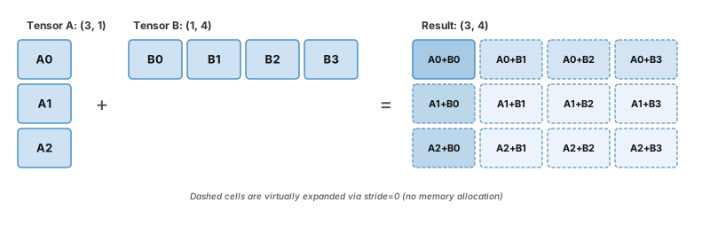
Consider a concrete case: tensor A has shape (32, 1, 64) and tensor B has shape (1, 128, 64). Comparing dimensions right to left, 64 matches 64, then 1 stretches to 128, then 1 stretches to 32, yielding result shape (32, 128, 64). Visualizing this expansion prevents silent logic bugs that accidentally allocate a large tensor (for example, a (Batch, Batch) matrix instead of an element-wise (Batch) vector).
Shapes, strides, and broadcasting govern how tensors flow through a model’s forward pass. Training adds a second requirement: learning from errors. Backpropagation makes that learning possible and imposes the memory costs developed below.
Mechanics of Learning
Valid tensor programs make training loops possible. Backpropagation orchestrates these tensors to compute gradients, transforming a forward prediction into a backward learning signal.
Systems Perspective 1.2: Why this matters
The chain rule and automatic differentiation
For a composed function \(y = f(g(x))\), the derivative is \(\frac{dy}{dx} = \frac{dy}{dg} \cdot \frac{dg}{dx}\). In a neural network, \(f\) and \(g\) are layers, and the composition can be many levels deep. For a three-layer network \(y = f_3(f_2(f_1(x)))\), the chain rule extends to: \[ \frac{\partial y}{\partial x} = \frac{\partial f_3}{\partial f_2} \cdot \frac{\partial f_2}{\partial f_1} \cdot \frac{\partial f_1}{\partial x} \]
Each factor in this product is a local derivative—computed at one layer using only that layer’s inputs and outputs. This locality is what makes the algorithm tractable: the entire network never needs to be differentiated as a monolithic function. Instead, each layer computes its own local derivative during the backward pass and multiplies it by the gradient flowing in from the layer above.
Modern frameworks use reverse-mode automatic differentiation, which computes gradients for all \(P\) parameters in a single backward pass. The key insight is that starting from the output and working backward (reverse mode) requires one pass regardless of the number of parameters, whereas starting from each input and working forward (forward mode) would require \(P\) passes—one per parameter. This is why a training step is a small constant multiple of inference, commonly about 2–3\(\times\) a forward pass for dense networks, rather than \(P\) passes.
The backpropagation algorithm
Backpropagation3 implements the chain rule efficiently through two passes: forward to compute outputs, backward to compute gradients. Figure 2 illustrates this process for a simple two-layer network, with the forward pass (gray arrows) computing outputs and the backward pass (red dashed arrows) propagating gradients.
3 Backpropagation: Short for “backward propagation of errors.” The algorithm was independently discovered multiple times—by Werbos (1974) and Linnainmaa (1970) for reverse-mode differentiation and by Rumelhart et al. (1986) for neural network training. Its key insight is that computing gradients for all parameters requires one backward pass through the graph rather than one pass per parameter. Section 1.4 derives the constant-factor work bound and a representative dense-layer cost.
\begin{tikzpicture}[font=\small\sffamily, node distance=3cm, auto, >=stealth, thick]
  \tikzset{
    Node/.style={circle, draw=BlueLine, fill=BlueFill, line width=0.8pt, minimum size=0.9cm, text=TextBlack},
    Edge/.style={->, draw=GrayLine, line width=0.8pt},
    BackEdge/.style={->, dashed, draw=RedLine, line width=0.8pt, bend right=30},
    Label/.style={font=\footnotesize\sffamily, text=TextBlack}
  }
  \node[Node] (x) {x};
  \node[Node, right of=x] (h) {h};
  \node[Node, right of=h] (y) {y};
  \node[Node, right of=y, fill=RedLine!10, draw=RedLine] (L) {$\mathcal{L}$};
  \draw[Edge] (x) -- node[below, Label] {$W_1$} (h);
  \draw[Edge] (h) -- node[below, Label] {$W_2$} (y);
  \draw[Edge] (y) -- node[below, Label] {Loss} (L);
  \draw[BackEdge,overlay] (L) to node[above, Label, text=RedLine] {$\frac{\partial \mathcal{L}}{\partial y}$} (y);
  \draw[BackEdge,overlay] (y) to node[above, Label, text=RedLine] {$\frac{\partial \mathcal{L}}{\partial h}$} (h);
  \draw[BackEdge,overlay] (h) to node[above, Label, text=RedLine] {$\frac{\partial \mathcal{L}}{\partial x}$} (x);
 \path[use as bounding box] (-0.5,-0.55) rectangle (9.5,1.21);
\end{tikzpicture}The gradient edges retrace the forward dependencies, so each backward step requires values retained from the corresponding forward operation.
Forward pass
Using row-vector activations, omitting biases, and retaining intermediate activations for backward, start at \(x\), the input. Multiply by \(W_1\) to get hidden activation \(h\). Cache \(h\) because the backward pass will need it later. Multiply \(h\) by \(W_2\) to get output \(y\). Cache \(y\). Compare \(y\) to the target label to compute loss \(\mathcal{L}\).
At this point, the loss has been computed and memory contains the input \(x\), the cached activation \(h\), the cached output \(y\), and the loss \(\mathcal{L}\). For a large model, these cached activations can dominate memory usage.
Backward pass
Now trace backward from \(\mathcal{L}\). The loss function provides \(\frac{\partial \mathcal{L}}{\partial y}\), the gradient of loss with respect to the prediction. This is where the error signal enters the network.
Since \(y = h \cdot W_2\), the chain rule gives us two gradients at this layer: \[ \frac{\partial \mathcal{L}}{\partial W_2} = h^T \cdot \frac{\partial \mathcal{L}}{\partial y} \qquad \text{(weight gradient—used to update } W_2\text{)} \] \[ \frac{\partial \mathcal{L}}{\partial h} = \frac{\partial \mathcal{L}}{\partial y} \cdot W_2^T \qquad \text{(input gradient—passed backward to the previous layer)} \]
Computing \(\frac{\partial \mathcal{L}}{\partial W_2}\) requires the cached activation \(h\) from the forward pass. Activations must remain available during backward because every layer’s weight gradient depends on that layer’s input.
Now continue backward to the first layer. Since \(h = x \cdot W_1\), the same pattern gives: \[ \frac{\partial \mathcal{L}}{\partial W_1} = x^T \cdot \frac{\partial \mathcal{L}}{\partial h} \]
Each step backward requires two things: the gradient flowing in from above \(\left(\frac{\partial \mathcal{L}}{\partial h}\right)\) and that layer’s input (\(x\)), which must be available during backward. This is why the backward pass costs roughly 2\(\times\) the forward pass in compute: at each layer, it performs two matrix multiplications (one for the weight gradient, one for the input gradient) vs. one in the forward pass.
The true cost of training memory
A common mistake is to assume that training memory equals model size. This assumption leads to immediate OOM errors because weights are only one of four components. Training memory comprises weights, gradients, optimizer state, and retained activations: \[ M_{\text{total}} = M_{\text{weights}} + M_{\text{gradients}} + M_{\text{optimizer}} + M_{\text{activations}} \]
For a standard Adaptive Moment Estimation (Adam) optimizer (Kingma and Ba 2015) in mixed precision (Micikevicius et al. 2017):
- Weights: 2 bytes (FP16/BF16) or 4 bytes (FP32).
- Gradients: Same size as weights.
- Optimizer State: Adam moments require 8 bytes per parameter; an FP32 master copy adds another 4 bytes, giving 8–12 bytes per parameter.
- Activations: The hidden giant. A recomputation- or tiled-attention-friendly estimate scales as \(\mathcal{O}(B \times S \times N_L \times d)\); a full no-recompute attention implementation also materializes attention-score tensors that scale with \(S^2\).
To see how these components interact in practice, consider a concrete model.
Napkin Math 1.1: Worked example: GPT-2 (1.5B) training memory
Model state (fixed per step):
- Weights (BF16): \(1.5 \times 10^{9}\) \(\times\) 2 bytes = 3 GB
- Gradients (BF16): \(1.5 \times 10^{9}\) \(\times\) 2 bytes = 3 GB
- Optimizer (FP32 master + momentum + variance): \(1.5 \times 10^{9}\) \(\times\) 12 bytes = 18 GB
- Total model state: 24 GB—fits on an 80 GB-class A100/H100 (85.9 GB in decimal units), but leaves only 61.9 GB for activations.
Activations (scale with batch):
Per-layer retained activations for this quick estimate are approximately \(12 \times B \times S \times d\) BF16 elements, or \(12 \times B \times S \times d \times 2\) bytes, where \(B\) is batch size and \(S\) is sequence length. The factor twelve accounts for the major intermediate tensors retained for backpropagation: input activations, QKV projections (\(3d\)), attention output, FFN intermediate (\(4d\)), and layer norm/dropout masks. This estimate assumes the implementation does not retain the full \(B \times N_{\text{heads}} \times S^2\) attention-score tensor, as in recomputation- or tiled-attention-friendly accounting. With 48 layers, batch size 8, and sequence length 1024:
\[48 \times 12 \times 8 \times 1024 \times 1600 \times 2\text{ bytes } \approx 15.1 GB\]
Systems insight: ~39.1 GB under this activation-accounting convention, which fits on one 85.9 GB accelerator. However, increase the batch to 64 and activations grow to ~120.8 GB, exceeding the remaining capacity. This is the threshold where gradient checkpointing or another memory-saving method becomes necessary; its savings and recomputation overhead depend on checkpoint placement and implementation.
Activation explosion
While weights are fixed (\(\mathcal{O}(P)\)), activations grow linearly with batch size and at least linearly with sequence length; implementations that materialize attention scores add an \(\mathcal{O}(S^2)\) component. As the worked example shows, activation memory can quickly exceed the room left after model state. Gradient checkpointing4 reduces this pressure by storing only selected activations and recomputing the rest during backpropagation (Chen et al. 2016); techniques such as FlashAttention address related attention-memory bottlenecks by tiling attention to reduce memory round-trips (Dao et al. 2022).
4 Gradient checkpointing: Trades compute for memory. Instead of storing all activations, only a subset (checkpoints) is kept, and the missing ones are recomputed during the backward pass. This reduces memory usage from storing every layer activation to roughly the square root of the layer count at the cost of ~33 percent more compute (Chen et al. 2016).
The same decomposition provides a quick feasibility check: sum the per-parameter model state, add the activation term implied by batch size and sequence length, and compare the total against the accelerator’s capacity.
Computational graphs and optimization
The dependency structure exposed by backpropagation also gives compilers something to optimize. ML compilers represent models as directed acyclic graphs (DAGs), and that representation enables hardware-independent transformations.
Static single assignment
Compilers transform graphs into static single-assignment (SSA) form, where each variable is assigned exactly once. This makes data dependencies explicit, enabling safe optimizations—most importantly, operator fusion.
Operator fusion
Without fusion, each operation in a chain like MatMul → Add (bias) → ReLU produces an intermediate tensor that is written to HBM and then read back for the next operation. For elementwise operations like Add and ReLU, the compute is trivial (one FLOP per element) but the memory traffic is not (read the tensor, write it back). The arithmetic intensity of unfused elementwise operations is therefore close to zero—deeply memory bound.
Fusion combines consecutive operations into a single kernel that reads the input once, applies all operations in registers or shared memory, and writes the final result once. For a sequence of \(k\) elementwise operations on a tensor of size \(N\) bytes, fusion reduces memory traffic from \(2kN\) bytes (each op reads and writes) to \(2N\) bytes (one read, one write)—a \(k\times\) reduction.
FlashAttention is an I/O-aware tiled attention algorithm: it computes the score, softmax, and value-product stages in SRAM tiles without materializing the full attention matrix in HBM, reducing HBM traffic and auxiliary attention memory from \(\mathcal{O}(S^2)\) to \(\mathcal{O}(S)\). The original work reports up to 3\(\times\) wall-clock speedups on its evaluated workloads (Dao et al. 2022); realized gains depend on shape and hardware (see section 1.5 for the step-by-step derivation). Together, the linear algebra foundations, tensor programming mechanics, and training memory model covered in this appendix form the algorithmic substrate on which all ML systems are built.
Baur–Strassen Reverse-Mode AD Complexity Theorem
Modern deep learning scales to hundreds of billions of parameters because evaluating the full gradient vector \(\nabla f(x)\) of a scalar loss function \(f: \mathbb{R}^N \to \mathbb{R}\) requires compute proportional to evaluating \(f(x)\) itself, with a constant-factor bound independent of the input dimension \(N\). Baur and Strassen proved this complexity result in 1983 (Baur and Strassen 1983).
Mathematical formulation and theorem statement
Let \(f: \mathbb{R}^N \to \mathbb{R}\) be a multivariate scalar-valued function represented as a computational graph \(G = (V, E)\) consisting of \(W(f)\) elementary operations (additions, subtractions, multiplications, divisions, and unary functions such as \(\exp, \ln, \sin, \sqrt{\cdot}\)).
Theorem 1.1: Baur–Strassen complexity theorem
Step-by-step chain rule adjoint graph propagation proof
Let the computational graph \(G = (V, E)\) be topologically ordered with nodes \(v_{1-N}, \dots, v_0, v_1\), \(v_2, \dots, v_W\), where input variables are \(x_i = v_{i-N}\) for \(i \in \{1, \dots, N\}\) and the final output is \(f(x) = v_W\). Each intermediate node \(v_j\) is evaluated via a primitive operation: \[ v_j = \phi_j\left( \{ v_k \mid k \in \text{Parents}(j) \} \right) \]
Define the adjoint variable \(\bar{v}_i\) for every node \(v_i\) as the partial derivative of the scalar output \(v_W\) with respect to \(v_i\): \[ \bar{v}_i \triangleq \frac{\partial f}{\partial v_i} = \frac{\partial v_W}{\partial v_i} \]
By the multivariate chain rule, the adjoint \(\bar{v}_i\) is the sum of partial derivatives propagated from all successor nodes (children) that consume \(v_i\): \[ \bar{v}_i = \sum_{j \in \text{Children}(i)} \bar{v}_j \cdot \frac{\partial v_j}{\partial v_i} \]
Reverse-mode automatic differentiation initializes \(\bar{v}_W = 1\) and \(\bar{v}_i = 0\) for all \(i < W\), then traverses the nodes in reverse topological order from \(v_W\) down to \(v_1\). For each primitive node \(v_j\), its fully accumulated adjoint \(\bar{v}_j\) propagates error signals to its parent nodes \(v_k\) (\(k \in \text{Parents}(j)\)) via: \[ \bar{v}_k \gets \bar{v}_k + \bar{v}_j \cdot \frac{\partial v_j}{\partial v_k} \]
We now perform operation-by-operation micro-cost accounting for all primitive nodes to bound the backward work:
- Addition/Subtraction (\(v_j = v_i \pm v_k\)):
- Local derivatives: \(\frac{\partial v_j}{\partial v_i} = 1\), \(\frac{\partial v_j}{\partial v_k} = \pm 1\).
- Backward updates: \(\bar{v}_i \gets \bar{v}_i + \bar{v}_j\) and \(\bar{v}_k \gets \bar{v}_k \pm \bar{v}_j\).
- Cost: 2 additions in backward pass for 1 forward operation. Work ratio: \(\text{Fwd}(1) + \text{Bwd}(2) = 3 \text{ OPs} \le 5 \cdot 1\).
- Multiplication (\(v_j = v_i \cdot v_k\)):
- Local derivatives: \(\frac{\partial v_j}{\partial v_i} = v_k\), \(\frac{\partial v_j}{\partial v_k} = v_i\).
- Backward updates: \(\bar{v}_i \gets \bar{v}_i + \bar{v}_j \cdot v_k\) and \(\bar{v}_k \gets \bar{v}_k + \bar{v}_j \cdot v_i\).
- Cost: 2 multiplications + 2 additions = 4 operations in backward pass for 1 forward operation. Work ratio: \(\text{Fwd}(1) + \text{Bwd}(4) = 5 \text{ OPs} \le 5 \cdot 1\).
- Division (\(v_j = v_i/v_k\)):
- Local derivatives: \(\frac{\partial v_j}{\partial v_i} = \frac{1}{v_k}\), \(\frac{\partial v_j}{\partial v_k} = -\frac{v_i}{v_k^2} = -\frac{v_j}{v_k}\).
- Backward updates: \(\bar{v}_i \gets \bar{v}_i + \frac{\bar{v}_j}{v_k}\) and \(\bar{v}_k \gets \bar{v}_k - \frac{\bar{v}_j \cdot v_j}{v_k}\).
- Cost: 2 multiplications/divisions + 2 additions = 4 operations in backward pass for 1 forward operation. Work ratio: \(\text{Fwd}(1) + \text{Bwd}(4) = 5 \text{ OPs} \le 5 \cdot 1\).
- Unary Transcendental Operations (\(v_j = \phi(v_i)\)):
- Local derivative: \(\frac{\partial v_j}{\partial v_i} = \phi'(v_i)\).
- Backward update: \(\bar{v}_i \gets \bar{v}_i + \bar{v}_j \cdot \phi'(v_i)\).
- For \(v_j = \exp(v_i)\), \(\phi'(v_i) = v_j\), requiring 1 multiplication + 1 addition = 2 OPs.
- For \(v_j = \ln(v_i)\), \(\phi'(v_i) = 1/v_i\), requiring 1 division + 1 addition = 2 OPs.
Summing across all primitive nodes in \(G\), every forward operation generates at most 4 backward operations: \[ \text{Work}_{\text{Backward}}(\nabla f) \le 4 \cdot W(f) \]
Adding the forward pass work \(W(f)\) yields the total work bound: \[ \text{Work}_{\text{Reverse}}(f, \nabla f) = W(f) + \text{Work}_{\text{Backward}}(\nabla f) \le 5 \cdot W(f) \qquad\blacksquare\]
Systems Perspective 1.3: Why 175B-parameter large language models can be trained
- Forward Pass: Matrix multiplications \(Y = X W\) require \(2P\) FLOPs per token.
- Reverse-Mode Backward Pass: Computes both weight gradients \(\frac{\partial \mathcal{L}}{\partial W} = X^T \frac{\partial \mathcal{L}}{\partial Y}\) (\(2P\) FLOPs) and input activation gradients \(\frac{\partial \mathcal{L}}{\partial X} = \frac{\partial \mathcal{L}}{\partial Y} W^T\) (\(2P\) FLOPs), totaling \(4P\) FLOPs per token.
- Total Training Work: \(2P (\text{fwd}) + 4P (\text{bwd}) = 6P\) FLOPs per token. The backward compute factor is exactly \(\frac{4P}{2P} = 2\), well within the Baur–Strassen theoretical bound of \(C \le 5\).
If we instead used forward-mode AD or finite differences to compute \(\nabla f \in \mathbb{R}^P\), evaluating each partial derivative separately would require \(P\) forward passes: \(\text{Work}_{\text{ForwardMode}}(\nabla f) = \mathcal{O}(P \cdot W) = \mathcal{O}(P^2)\) FLOPs. For \(P = 175 \times 10^9\), that method would require \(2 \times (175 \times 10^9)^2 \approx 6.1 \times 10^{22}\) FLOPs per token—\(P\) times the forward-pass work and therefore prohibitive at this scale. Reverse-mode AD collapses this \(\mathcal{O}(P)\) factor into a constant multiplier of 2 for the dense-layer accounting above.
FlashAttention Tiling & Online Softmax Recurrence Proof
Standard self-attention in transformers requires materializing an \(N \times N\) attention score matrix in HBM, creating an \(\mathcal{O}(N^2)\) memory bandwidth bottleneck. FlashAttention (Dao et al. 2022) eliminates this bottleneck by tiling query, key, and value matrices and recomputing attention using an online softmax recurrence without materializing intermediate scores to HBM.
Standard softmax HBM I/O bottleneck
Given queries \(\mathbf{Q} \in \mathbb{R}^{N \times d}\), keys \(\mathbf{K} \in \mathbb{R}^{N \times d}\), and values \(\mathbf{V} \in \mathbb{R}^{N \times d}\) for sequence length \(N\) and head dimension \(d\), standard attention evaluates: \[ \mathbf{S} = \mathbf{Q} \mathbf{K}^T \in \mathbb{R}^{N \times N}, \qquad \mathbf{A} = \text{softmax}(\mathbf{S}) \in \mathbb{R}^{N \times N}, \qquad \mathbf{O} = \mathbf{A} \mathbf{V} \in \mathbb{R}^{N \times d} \]
To prevent numerical overflow, row-wise softmax subtracts the row maximum \(m_i = \max_{1 \le j \le N} S_{ij}\): \[ A_{ij} = \frac{\exp(S_{ij} - m_i)}{\sum_{k=1}^N \exp(S_{ik} - m_i)} \]
Standard GPU implementations execute this in three discrete kernel launches:
- Compute \(\mathbf{S} = \mathbf{Q}\mathbf{K}^T\) in SRAM, then write \(\mathbf{S} \in \mathbb{R}^{N \times N}\) to HBM (\(\Theta(N^2)\) writes).
- Read \(\mathbf{S}\) from HBM, compute row max \(m\) and row sum \(d\), compute \(\mathbf{A} = \text{softmax}(\mathbf{S})\), write \(\mathbf{A} \in \mathbb{R}^{N \times N}\) to HBM (\(\Theta(N^2)\) reads + writes).
- Read \(\mathbf{A}\) and \(\mathbf{V}\) from HBM, compute \(\mathbf{O} = \mathbf{A}\mathbf{V}\), write \(\mathbf{O} \in \mathbb{R}^{N \times d}\) to HBM (\(\Theta(N^2 + Nd)\) reads + writes).
Total HBM memory traffic is \(\Theta(N^2 + Nd)\) elements. For \(N = 8192\), \(d = 128\) in FP16, \(\mathbf{S}\) requires \(8192^2 \times 2 \text{ B} = 134 \text{ MB}\) per head per layer. Because modern GPUs feature massive compute throughput relative to HBM bandwidth, repeatedly reading and writing intermediate matrices \(\mathbf{S}\) and \(\mathbf{A}\) leaves GPU execution units memory-bound.
Online softmax recurrence proof
Tiling softmax is difficult because computing \(d_i = \sum_{k=1}^N \exp(S_{ik} - m_i)\) requires the global maximum \(m_i\) across all \(N\) keys. The online softmax recurrence solves this by incrementally updating normalization statistics as sub-blocks arrive.
Theorem 1.2: Online softmax recurrence theorem
Then the combined maximum \(m^{\text{new}}\), normalization sum \(d^{\text{new}}\), and accumulated output vector \(\mathbf{O}^{\text{new}}\) satisfy the exact recurrence relations: \[ m^{\text{new}} = \max\left(m^{(1)}, m^{(2)}\right) \] \[ d^{\text{new}} = d^{(1)} e^{m^{(1)} - m^{\text{new}}} + d^{(2)} e^{m^{(2)} - m^{\text{new}}} \] \[ \mathbf{O}^{\text{new}} = \frac{d^{(1)} e^{m^{(1)} - m^{\text{new}}}}{d^{\text{new}}} \mathbf{O}^{(1)} + \frac{e^{m^{(2)} - m^{\text{new}}}}{d^{\text{new}}} \sum_{j=1}^{N_2} e^{x_j^{(2)} - m^{(2)}} \mathbf{V}_j^{(2)} \] where \(\mathbf{O}^{(1)} = \frac{1}{d^{(1)}} \sum_{j=1}^{N_1} e^{x_j^{(1)} - m^{(1)}} \mathbf{V}_j^{(1)}\) is the partial output accumulated from block 1.
Derivation of denominator recurrence
Expanding the combined sum \(d^{\text{new}} = \sum_{j=1}^N e^{x_j - m^{\text{new}}}\): \[ \begin{aligned} d^{\text{new}} &= \sum_{j=1}^{N_1} e^{x_j^{(1)} - m^{\text{new}}} + \sum_{j=1}^{N_2} e^{x_j^{(2)} - m^{\text{new}}} \\ &= \sum_{j=1}^{N_1} e^{\left(x_j^{(1)} - m^{(1)}\right) + \left(m^{(1)} - m^{\text{new}}\right)} + \sum_{j=1}^{N_2} e^{\left(x_j^{(2)} - m^{(2)}\right) + \left(m^{(2)} - m^{\text{new}}\right)} \\ &= e^{m^{(1)} - m^{\text{new}}} \underbrace{\sum_{j=1}^{N_1} e^{x_j^{(1)} - m^{(1)}}}_{d^{(1)}} + e^{m^{(2)} - m^{\text{new}}} \underbrace{\sum_{j=1}^{N_2} e^{x_j^{(2)} - m^{(2)}}}_{d^{(2)}} \\ &= d^{(1)} e^{m^{(1)} - m^{\text{new}}} + d^{(2)} e^{m^{(2)} - m^{\text{new}}}. \quad \blacksquare \end{aligned} \]
Derivation of output rescaling recurrence
The true normalized output over the concatenated sequence is \(\mathbf{O}^{\text{new}} = \frac{1}{d^{\text{new}}} \sum_{j=1}^N e^{x_j - m^{\text{new}}} \mathbf{V}_j\): \[ \begin{aligned} \mathbf{O}^{\text{new}} &= \frac{1}{d^{\text{new}}} \left[ \sum_{j=1}^{N_1} e^{x_j^{(1)} - m^{\text{new}}} \mathbf{V}_j^{(1)} + \sum_{j=1}^{N_2} e^{x_j^{(2)} - m^{\text{new}}} \mathbf{V}_j^{(2)} \right] \\ &= \frac{1}{d^{\text{new}}} \left[ e^{m^{(1)} - m^{\text{new}}} \sum_{j=1}^{N_1} e^{x_j^{(1)} - m^{(1)}} \mathbf{V}_j^{(1)} + e^{m^{(2)} - m^{\text{new}}} \sum_{j=1}^{N_2} e^{x_j^{(2)} - m^{(2)}} \mathbf{V}_j^{(2)} \right] \end{aligned} \]
Noting that \(d^{(1)} \mathbf{O}^{(1)} = \sum_{j=1}^{N_1} e^{x_j^{(1)} - m^{(1)}} \mathbf{V}_j^{(1)}\), we substitute this directly: \[ \mathbf{O}^{\text{new}} = \frac{d^{(1)} e^{m^{(1)} - m^{\text{new}}}}{d^{\text{new}}} \mathbf{O}^{(1)} + \frac{e^{m^{(2)} - m^{\text{new}}}}{d^{\text{new}}} \sum_{j=1}^{N_2} e^{x_j^{(2)} - m^{(2)}} \mathbf{V}_j^{(2)}. \quad \blacksquare \]
Formal HBM access complexity proof
Let \(M\) be the fast SRAM capacity (in words). Following Algorithm 1 of Dao et al. (2022), FlashAttention sets \(B_c = \lfloor M/(4d) \rfloor\) and \(B_r = \min(\lfloor M/(4d) \rfloor,d)\). The proof abstracts constant factors and buffer reuse, using \(B_c=\Theta(M/d)\), \(B_r=\Theta(\min(M/d,d))\), and \(B_rB_c=O(M)\) for the on-chip working set.
The algorithm executes two nested loops:
- Partition \(\mathbf{Q}\) into \(T_r = \lceil N/B_r \rceil\) blocks of size \(B_r \times d\).
- Partition \(\mathbf{K}, \mathbf{V}\) into \(T_c = \lceil N/B_c \rceil\) blocks of size \(B_c \times d\).
- Outer loop over \(j = 1, \dots, T_c\): Load \(\mathbf{K}_j\) and \(\mathbf{V}_j\) into SRAM.
- Inner loop over \(i = 1, \dots, T_r\): Load \(\mathbf{Q}_i\), \(\mathbf{O}_i\), and its softmax statistics; compute \(\mathbf{S}_{ij} = \mathbf{Q}_i \mathbf{K}_j^T\) in SRAM; then update and write \(\mathbf{O}_i\) and the statistics without materializing \(\mathbf{S}_{ij}\) in HBM.
This loop order is the source of the I/O reduction. A key-value tile remains resident while the algorithm visits every query tile, so each element of \(\mathbf{K}\) and \(\mathbf{V}\) crosses the HBM boundary once. The query and output tiles must be revisited for each key-value block, but the \(B_r\times B_c\) score tile is consumed on chip and discarded. Standard attention instead writes and rereads the full \(N\times N\) score and probability matrices.
Total memory access accounting
- Key and value reads: Each element of \(\mathbf{K}\) and \(\mathbf{V}\) is loaded once, contributing \(2Nd\) accesses.
- Query, output, and statistics passes: Each of the \(T_c\) column blocks reads all of \(\mathbf{Q}\), reads and writes \(\mathbf{O}\), and updates \(O(N)\) softmax statistics. The matrices dominate the statistics for head dimension \(d\geq 1\), so each pass contributes \(\Theta(Nd)\) accesses and all passes contribute \(\Theta(NdT_c)\).
Because \(T_c=\lceil N/B_c\rceil=\Theta(Nd/M)\), the total is \[ \text{HBM}_{\text{Flash}} = \Theta\left(Nd + NdT_c\right) = \Theta\left(Nd + \frac{N^2d^2}{M}\right) = \Theta\left(\frac{N^2d^2}{M}\right), \] where the final equality follows for \(d \leq M \leq Nd\).
The bound counts communication rather than arithmetic. FlashAttention still evaluates the same dense score blocks and may recompute intermediate quantities during backpropagation; its advantage comes from keeping those intermediates out of HBM.
I/O reduction ratio
Comparing standard attention I/O to FlashAttention I/O: \[ \frac{\text{HBM}_{\text{Standard}}}{\text{HBM}_{\text{Flash}}} = \frac{\Theta(N^2 + Nd)}{\Theta\left(Nd + \frac{N^2 d^2}{M}\right)} = \Theta\left(\frac{M}{d^2}\right) \quad \text{for } N \gg \max\left(d,\frac{M}{d}\right) \]
Systems Perspective 1.4: A100 I/O reduction
- Standard attention: 35.3 GB of HBM reads and writes; 35.1 ms runtime.
- FlashAttention: 4.4 GB of HBM reads and writes; 11.7 ms runtime.
The measurements show the systems consequence of the I/O bound: substantially less HBM traffic coincides with lower runtime even though FlashAttention performs additional recomputation. They do not imply that every configuration becomes compute bound; tile size, sequence length, and kernel implementation determine the realized regime.
Kaplan & Chinchilla Compute-Optimal Scaling Law Derivation
Determining the compute-optimal allocation between model parameters \(N\) and training dataset tokens \(D\) for a given floating-point budget \(C\) is a central decision in large language model system design. This section provides the rigorous mathematical derivation of compute-optimal scaling laws using Lagrange multipliers, contrasting the original findings of Kaplan et al. (2020) with the compute-optimal corrections of Hoffmann et al. (2022).
Parametric loss surface formulation
The cross-entropy evaluation loss \(\mathcal{L}(N, D)\) of an autoregressive transformer language model trained with \(N\) non-embedding parameters on \(D\) tokens is modeled by the power-law formulation: \[ \mathcal{L}(N, D) = E + \frac{A}{N^\alpha} + \frac{B}{D^\beta} \] where:
- \(E\): Irreducible loss representing the entropy of natural language data.
- \(\frac{A}{N^\alpha}\): Capacity bottleneck loss resulting from finite model parameters \(N\).
- \(\frac{B}{D^\beta}\): Dataset size bottleneck loss resulting from finite training tokens \(D\).
- \(A, B > 0\): Empirical scaling constants.
- \(\alpha, \beta > 0\): Power-law scaling exponents for model size and dataset size, respectively.
Constrained optimization via Lagrange multipliers
The total floating-point operations required to train a transformer with \(N\) non-embedding parameters for \(D\) tokens is given by: \[ C = 6 N D \text{ FLOPs} \]
where \(2 N D\) accounts for the forward pass and \(4 N D\) accounts for the backward pass.
Given a fixed training compute budget \(C_0\), we formulate the constrained optimization problem to minimize the reducible loss \(\hat{\mathcal{L}}(N, D) = \frac{A}{N^\alpha} + \frac{B}{D^\beta}\): \[ \min_{N, D} \left( \frac{A}{N^\alpha} + \frac{B}{D^\beta} \right) \quad \text{subject to} \quad g(N, D) = 6 N D - C_0 = 0 \]
We construct the Lagrangian function \(\mathcal{L}_{\text{Lagrange}}(N, D, \lambda)\): \[ \mathcal{L}_{\text{Lagrange}}(N, D, \lambda) = \frac{A}{N^\alpha} + \frac{B}{D^\beta} + \lambda (6 N D - C_0) \]
Taking partial derivatives with respect to \(N, D\), and \(\lambda\) and setting them to zero: \[ \frac{\partial \mathcal{L}_{\text{Lagrange}}}{\partial N} = -\alpha A N^{-\alpha - 1} + 6 \lambda D = 0 \implies \alpha A N^{-\alpha - 1} = 6 \lambda D \tag{1} \] \[ \frac{\partial \mathcal{L}_{\text{Lagrange}}}{\partial D} = -\beta B D^{-\beta - 1} + 6 \lambda N = 0 \implies \beta B D^{-\beta - 1} = 6 \lambda N \tag{2} \] \[ \frac{\partial \mathcal{L}_{\text{Lagrange}}}{\partial \lambda} = 6 N D - C_0 = 0 \tag{3} \]
Multiplying Equation (1) by \(N\) and Equation (2) by \(D\): \[ \alpha A N^{-\alpha} = 6 \lambda N D \] \[ \beta B D^{-\beta} = 6 \lambda N D \]
Equating these expressions yields the fundamental power-law optimality condition: \[ \alpha A N^{-\alpha} = \beta B D^{-\beta} \]
This condition proves that at the compute-optimal allocation, the marginal loss reduction per fractional increase in parameter count must equal the marginal loss reduction per fractional increase in dataset tokens.
Analytical derivation of compute-optimal exponents
From \(\alpha A N^{-\alpha} = \beta B D^{-\beta}\), we solve for \(D\) in terms of \(N\): \[ D^\beta = \left(\frac{\beta B}{\alpha A}\right) N^\alpha \implies D = \left(\frac{\beta B}{\alpha A}\right)^{1/\beta} N^{\alpha/\beta} \]
Substituting \(D\) into the compute constraint \(C = 6 N D\): \[ C = 6 N \left(\frac{\beta B}{\alpha A}\right)^{1/\beta} N^{\alpha/\beta} = 6 \left(\frac{\beta B}{\alpha A}\right)^{1/\beta} N^{\frac{\alpha + \beta}{\beta}} \]
Solving explicitly for the compute-optimal parameter count \(N^*(C)\): \[ N^*(C) = \left( \frac{\alpha A}{\beta B} \right)^{\frac{1}{\alpha + \beta}} \left( \frac{C}{6} \right)^{\frac{\beta}{\alpha + \beta}} \propto C^{\frac{\beta}{\alpha + \beta}} \]
By symmetry, solving for the compute-optimal token count \(D^*(C)\): \[ D^*(C) = \left( \frac{\beta B}{\alpha A} \right)^{\frac{1}{\alpha + \beta}} \left( \frac{C}{6} \right)^{\frac{\alpha}{\alpha + \beta}} \propto C^{\frac{\alpha}{\alpha + \beta}} \]
Empirical exponents and the \(D/N \approx 20\) rule
Fitting the parametric loss surface to over 400 experimental runs, Hoffmann et al. (2022) estimated \(\alpha \approx 0.34\) and \(\beta \approx 0.28\). Substituting these values gives exponents close to the paper’s parametric-model result:
\[ \frac{\beta}{\alpha + \beta} \approx 0.45, \qquad \frac{\alpha}{\alpha + \beta} \approx 0.55 \]
Thus the parametric model predicts: \[ N^*(C) \propto C^{0.45}, \qquad D^*(C) \propto C^{0.55} \]
The paper’s two direct empirical approaches report near-balanced exponents of \((0.50, 0.50)\) and \((0.49, 0.51)\), which motivate the common square-root shorthand. Under the parametric fit, however, \(D^*/N^*\) grows slowly with compute rather than remaining strictly constant. Across the regime studied, roughly 20 training tokens per parameter is a useful Chinchilla heuristic, not a universal invariant.
Systems Perspective 1.5: Kaplan vs. Chinchilla scaling
The difference between Kaplan et al. (2020) and Hoffmann et al. (2022) highlights how hyperparameter choices in empirical benchmarking can alter system design conclusions:
- Kaplan et al. (2020) estimated \(\alpha \approx 0.057\) and \(\beta \approx 0.28\), predicting \(N \propto C^{0.73}\) and \(D \propto C^{0.27}\). This led the field to scale model sizes aggressively while holding training dataset sizes relatively small (e.g., GPT-3 175B trained on 300B tokens, giving \(D/N = 1.71\)).
- Methodological difference: Kaplan et al. (2020) used a fixed token budget and learning-rate schedule across models. Hoffmann et al. (2022) matched the schedule to each training horizon and found that the earlier setup understated the value of training smaller models on more data.
- Hoffmann et al. (2022) found near-balanced parameter and token scaling: its three approaches report exponent pairs of \((0.50, 0.50)\), \((0.49, 0.51)\), and \((0.46, 0.54)\) rather than one exact universal ratio.
- Practical Impact: Chinchilla (70B parameters trained on 1.4T tokens, \(D/N = 20\)) outperformed GPT-3 (175B parameters trained on 300B tokens) across downstream benchmarks while requiring \(2.5\times\) less compute during inference and \(2.5\times\) lower weight memory at the same precision (Hoffmann et al. 2022).
Summary
An algorithm becomes a systems workload through its shapes, operation graph, data dependencies, and numerical representation. Linear-algebra primitives, memory layouts, broadcasting, and sparse formats determine work, traffic, locality, and usable parallelism. Automatic differentiation and backpropagation add saved activations and backward computation; computational graphs then expose opportunities for fusion and recomputation. The Baur–Strassen result bounds reverse-mode overhead, while FlashAttention shows how tiling and an online recurrence can reduce HBM traffic without changing attention semantics.
The same accounting connects kernels to scaling decisions. Compute-optimal scaling turns a fixed budget into a model-data allocation, but the fitted exponents remain empirical rather than universal. Across these models, the reusable method is to expose operations, bytes, saved state, dependencies, and asymptotic constraints before selecting an optimization.