Deployment Paradigm Framework
ML Systems
Purpose
Why does deploying the same model to a phone vs. a data center demand fundamentally different engineering?
The defining insight of ML systems engineering is that constraints drive architecture. The speed of light sets an absolute floor on how quickly distant servers can respond. Thermodynamics limits how much computation can occur in a given volume before heat becomes unmanageable. Memory physics makes moving data often more expensive than processing it. These are not engineering limitations awaiting better technology; they are permanent physical boundaries that partition the world into fundamentally distinct operating regimes. A data center can train billion-parameter models but cannot guarantee low-latency responses to users thousands of miles away. A smartphone can respond instantly but has a fraction of the memory budget. A microcontroller can run on a coin-cell battery for years but has barely enough compute for a simple keyword detector. The same model, the same algorithm applied to the same data, demands radically different engineering in each regime, not because the physics changes but because different constraints dominate. Teams that treat deployment as an afterthought, training in one environment and deferring target constraints until launch, discover too late that the target environment invalidates months of architectural decisions. The engineering task is therefore not to identify a universally best deployment but to locate the constraint that binds in the intended operating regime. In D·A·M terms, understanding these regimes transforms deployment from an operational detail into a first-order co-design problem in which data locality, algorithm structure, and machine constraints jointly determine what is possible.
Learning Objectives
- Explain how physical constraints create deployment paradigms from cloud to TinyML
- Apply the iron law and bottleneck principle to classify compute-, memory-, and I/O-bound workloads
- Map workload archetypes to deployment paradigms using lighthouse model examples
- Compare cloud, edge, mobile, and TinyML by operational constraints and quantitative trade-offs
- Apply the decision framework to select paradigms by privacy, latency, compute, and cost constraints
- Analyze hybrid patterns that combine paradigms to satisfy system constraints
- Evaluate deployment decisions, common fallacies, and universal principles that transfer across scales
Consider two extremes: a wake-word detector on a smartwatch and a recommendation engine in a data center. The wake-word detector represents a TinyML workload operating under milliwatt power budgets and kilobyte memory limits; the recommendation engine exemplifies a cloud ML workload requiring terabytes of embedding tables and megawatt-scale infrastructure. These systems solve different problems under opposite physical constraints, and their supporting infrastructure differs sharply in scale and design. This reality transforms deployment from an operational afterthought into a first-order engineering decision, one that the D·A·M taxonomy shown in The D·A·M Intersection Landscape helps us reason about by foregrounding infrastructure alongside data and algorithms.
Physical constraints determine where an ML model can run and shape what is possible in ways no algorithmic choice can override. Yet deployment is far harder than it appears, and the reason is not the model itself. In production ML systems, the model is often only a small part of the overall system (Sculley et al. 2015). The surrounding infrastructure consists of data collection, feature processing, serving infrastructure, monitoring, and resource management. All of it changes dramatically depending on where the model executes.
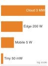
Power spans the paradigms from megawatts (cloud) to milliwatts (TinyML).
Shi, Weisong, Jie Cao, Quan Zhang, Youhuizi Li, and Lanyu Xu. 2016. “Edge Computing: Vision and Challenges.” IEEE Internet of Things Journal 3 (5): 637–46. https://doi.org/10.1109/jiot.2016.2579198.
The physical constraints that govern each environment (latency, power, and memory) force ML deployment into four distinct paradigms, each with its own engineering trade-offs and system design patterns. Cloud ML aggregates computational resources in data centers, offering elastic compute and large-scale storage at the cost of network latency. Edge ML moves computation closer to where data originates, reducing remote-path latency and limiting sensitive-data transmission (Shi et al. 2016). Mobile ML brings intelligence directly to smartphones and tablets, balancing computational capability against battery life and thermal constraints. TinyML pushes intelligence to microcontrollers costing dollars and consuming milliwatts (Janapa Reddi et al. 2022). The categorical envelope from megawatts to milliwatts spans nine orders of magnitude in power, while the representative systems in figure 1 span nearly eight. The figure positions five deployment tiers—from ultra-low-power sensors on the left to warehouse data centers on the right—delineating where TinyML, edge AI, and cloud AI operating envelopes overlap.
\begin{tikzpicture}[line cap=round,line join=round,font=\sffamily\small]
  % Parameters
  \def\angle{1.0}       % angle
  \def\length{20.5}     % Lengths (cm)
  \def\npoints{5}       % number of points
  \def\startfrac{0.13}  % start (e.g.. 0.2 = 20%)
  \def\endfrac{0.87}    % end (e.g.. 0.8 = 80%)

 \draw[line width=1pt, black!70] (0,0) -- ({\length*cos(\angle)}, {\length*sin(\angle)})coordinate(end);
 %
  \foreach \i in {0,1,...,\numexpr\npoints-1} {
    \pgfmathsetmacro{\t}{\startfrac + (\endfrac - \startfrac)*\i/(\npoints-1)}
\coordinate(T\i)at({\t*\length*cos(\angle)}, {\t*\length*sin(\angle)});
  }

\tikzset {
pics/gatewey/.style = {
        code = {
\colorlet{red}{white}
\begin{scope}[local bounding box=GAT,scale=0.9, every node/.append style={transform shape}]
\def\rI{4mm}
\def\rII{2.8mm}
\def\rIII{1.6mm}
\draw[red,line width=1.25pt](0,0)--(0,0.38)--(1.2,0.38)--(1.2,0)--cycle;
\draw[red,line width=1.5pt](0.6,0.4)--(0.6,0.9);

\draw[red, line width=1.5pt] (0.6,0.9)+(60:\rI) arc[start angle=60, end angle=-60, radius=\rI];
\draw[red, line width=1.5pt] (0.6,0.9)+(50:\rII) arc[start angle=50, end angle=-50, radius=\rII];
\draw[red, line width=1.5pt] (0.6,0.9)+(30:\rIII) arc[start angle=30, end angle=-30, radius=\rIII];
%
 \draw[red, line width=1.5pt] (0.6,0.9)+(120:\rI) arc[start angle=120, end angle=240, radius=\rI];
\draw[red, line width=1.5pt] (0.6,0.9)+(130:\rII) arc[start angle=130, end angle=230, radius=\rII];
\draw[red, line width=1.5pt] (0.6,0.9)+(150:\rIII) arc[start angle=150, end angle=210, radius=\rIII];
\fill[red](0.6,0.9)circle (1.5pt);

\foreach\i in{0.15,0.3,0.45,0.6}{
\fill[red](\i,0.19)circle (1.5pt);
}

\fill[red](1,0.19)circle (2pt);
\end{scope}
}}}

\tikzset {
pics/cloud/.style = {
        code = {
\colorlet{red}{white}
\begin{scope}[local bounding box=CLO,scale=0.6, every node/.append style={transform shape}]
\draw[red,line width=1.5pt](0,0)to[out=170,in=180,distance=11](0.1,0.61)
to[out=90,in=105,distance=17](1.07,0.71)
to[out=20,in=75,distance=7](1.48,0.36)
to[out=350,in=0,distance=7](1.48,0)--(0,0);
\draw[red,line width=1.5pt](0.27,0.71)to[bend left=25](0.49,0.96);
\draw[red,line width=1.5pt](0.67,1.21)to[out=55,in=90,distance=13](1.5,0.96)
to[out=360,in=30,distance=9](1.68,0.42);
\end{scope}
}}}

\tikzset {
  pics/server/.style = {
    code = {
      \colorlet{red}{white}
      \begin{scope}[anchor=center, transform shape,scale=0.8, every node/.append style={transform shape}]
        \draw[red,line width=1.25pt,fill=white](-0.55,-0.5) rectangle (0.55,0.5);
\foreach \i in {-0.25,0,0.25} {
                \draw[BlueLine,line width=1.25pt]( -0.55,\i) -- (0.55, \i);
}
        \foreach \i in {-0.375, -0.125, 0.125, 0.375} {
          \draw[BlueLine,line width=1.25pt](-0.45,\i)--(0,\i);
          \fill[BlueLine](0.35,\i) circle (1.5pt);
        }

\draw[red,line width=1.75pt](0,-0.53) |- (-0.55,-0.7);
        \draw[red,line width=1.75pt](0,-0.53) |- (0.55,-0.7);
      \end{scope}
    }
  }
}

\tikzset {
pics/cpu/.style = {
        code = {
\definecolor{CPU}{RGB}{0,120,176}
\colorlet{CPU}{white}
\begin{scope}[local bounding box = CPU,scale=0.33, every node/.append style={transform shape}]
\node[fill=CPU,minimum width=66, minimum height=66,
            rounded corners=2,outer sep=2pt] (C1) {};
\node[fill=violet,minimum width=54, minimum height=54] (C2) {};
%\node[fill=CPU!40,minimum width=44, minimum height=44] (C3) {CPU};

\foreach \x/\y in {0.11/1,0.26/2,0.41/3,0.56/4,0.71/5,0.85/6}{
\node[fill=CPU,minimum width=4, minimum height=15,
           inner sep=0pt,anchor=south](GO\y)at($(C1.north west)!\x!(C1.north east)$){};
}
\foreach \x/\y in {0.11/1,0.26/2,0.41/3,0.56/4,0.71/5,0.85/6}{
\node[fill=CPU,minimum width=4, minimum height=15,
           inner sep=0pt,anchor=north](DO\y)at($(C1.south west)!\x!(C1.south east)$){};
}
\foreach \x/\y in {0.11/1,0.26/2,0.41/3,0.56/4,0.71/5,0.85/6}{
\node[fill=CPU,minimum width=15, minimum height=4,
           inner sep=0pt,anchor=east](LE\y)at($(C1.north west)!\x!(C1.south west)$){};
}
\foreach \x/\y in {0.11/1,0.26/2,0.41/3,0.56/4,0.71/5,0.85/6}{
\node[fill=CPU,minimum width=15, minimum height=4,
           inner sep=0pt,anchor=west](DE\y)at($(C1.north east)!\x!(C1.south east)$){};
}
\end{scope}
    }  }}

\tikzset {
pics/mobile/.style = {
        code = {
\colorlet{red}{white}
\begin{scope}[local bounding box=MOB,scale=0.4, every node/.append style={transform shape}]
\node[rectangle,draw=red,minimum height=94,minimum width=47,
            rounded corners=6,thick,fill=white](R1){};
\node[rectangle,draw=red,minimum height=67,minimum width=38,thick,fill=GreenFill](R2){};
\node[circle,minimum size=8,below= 2pt of R2,inner sep=0pt,thick,fill=GreenFill]{};
\node[rectangle,fill=GreenFill,minimum height=2,minimum width=20,above= 4pt of R2,inner sep=0pt,thick]{};
%
 \end{scope}
     }  }}

\node[draw=none,fill=RedFill,circle,minimum size=20mm](GA)at(T2){};
\pic[shift={(-0.55,-0.5)}] at (T2) {gatewey};
\node[above=0 of GA]{Gateway};
\node[draw=none,fill=VioletL,circle,minimum size=20mm](CP)at(T0){};
\pic[shift={(0,-0)}] at (T0) {cpu};
\node[above=0 of CP,align=center]{Ultra-Low-Power\\Devices and Sensors};
\node[draw=none,fill=GreenFill,,circle,minimum size=20mm](MO)at(T1){};
 \pic[shift={(0,0)}] at (T1) {mobile};
 \node[above=0 of MO,align=center]{Intelligent Device};
\node[draw=none,fill=BlueFill,circle,minimum size=20mm](SE)at(T3){};
\pic[shift={(-0.03,0.1)}] at (T3) {server};
 \node[above=0 of SE,align=center]{On-Premises Servers};
\node[draw=none,fill=BrownL,circle,minimum size=20mm](CL)at(T4){};
\pic[shift={(-0.48,-0.35)}] at (T4) {cloud};
 \node[above=0 of CL,align=center]{Cloud};
%
\path (T0) -- (T1) coordinate[pos=0.5] (M1);
\path (0,0) -- (T0) coordinate[pos=0.25] (M0);
\path (T3) -- (T4) coordinate[pos=0.5] (M2);
\path (T4) -- (end) coordinate[pos=0.75] (M3);

\foreach \x in {0,1,2,3}{
\fill[OliveLine](M\x)circle (2.5pt);
}

\path[red](M0)--++(270:1.6)coordinate(LL1)-|coordinate(LL2)(M2);
\path[red](M0)--++(270:1.25)coordinate(L1)-|coordinate(L2)(M1);
\path[red](M0)--++(270:1.1)-|coordinate(L3)(M2);
\path[red](M0)--++(270:1.1)-|coordinate(L4)(M3);
%
\draw[black!70,thick](M0)--(LL1);
\draw[black!70,thick](M1)--(L2);
\draw[black!70,thick](M3)--(L4);
\draw[black!70,thick](M2)--(LL2);
\draw[latex-latex,line width=1pt,draw=black!60](L1)--node[red,fill=white]{TinyML}(L2);
\draw[latex-latex,line width=1pt,draw=black!60](L3)--node[fill=white]{Cloud AI}(L4);
\draw[latex-latex,line width=1pt,draw=black!60]([yshift=4pt]LL1)--node[fill=white,text=black]{Edge AI}([yshift=4pt]LL2);
\foreach \x in {0,1,2,3}{
\fill[OliveLine](M\x)circle (2.5pt);
}
%
\path[](M0)--++(90:1.9)-|node[pos=0.25]{\textbf{The Distributed Intelligence Spectrum}}(M3);
\end{tikzpicture}While figure 1 illustrates the qualitative topology of distributed intelligence, table 1 quantifies the operational envelopes across processing location, round-trip latency, power draw, and memory capacity. This nine-order-of-magnitude power span reflects three inescapable physical boundaries: the speed of light (establishing latency floors), thermodynamic dissipation limits (capping computation per watt), and memory signaling energy (the memory wall).
| Paradigm | Where | Latency (ms) | Power | Memory | Best For |
|---|---|---|---|---|---|
| Cloud ML | Data centers | 100-500 | MW | TB | Training, complex inference |
| Edge ML | Local servers | 10-100 | 100 W | GB | Real-time inference, privacy |
| Mobile ML | Smartphones | 5-50 | 3–5 W | GB | Personal AI, offline |
| TinyML | Microcontrollers | 1-10 | mW | KB | Always-on sensing |
The architectural anchor: The single-node stack
To navigate these operating regimes, we anchor our engineering decisions in a four-layer model of the single-node stack, which refines the machine side of the D·A·M taxonomy for one host while data and algorithm enter through workload requirements. At the top of the stack, the application defines the mission through a training-throughput or inference-latency target. Model Training and Model Serving develop the mechanisms that determine whether the system can meet it. The ML framework translates model code into executable operations (ML Frameworks). The operating system orchestrates resources and moves data between host memory and accelerator memory. The hardware itself, defined by high-bandwidth memory (HBM) capacity, memory bandwidth, intra-node interconnects such as NVLink, and compute throughput, sets the physical limits, with the memory wall as a recurring constraint (Hardware Acceleration).
This stack establishes the chapter’s silicon contract: the fixed performance bargain a given piece of silicon offers a model, set by memory bandwidth, peak compute rate, and fixed overhead. Every chapter in the first half of this text interrogates one or more of these layers, because understanding how they interact within a single machine is the technical prerequisite for mastering larger distributed scales.
These physical constraints interact with the iron law of ML systems (Iron Law of ML Systems), which decomposes end-to-end latency into data movement, computation, and overhead. Different deployment environments emphasize different constraints: cloud training can be compute bound, mobile systems face power walls, and TinyML devices often reach memory-capacity limits. By pairing the physical constraints with the iron law, we develop a quantitative vocabulary for reasoning about which paradigm fits a given workload and why. To anchor this analysis concretely, the chapter introduces five lighthouse models (ResNet-50, GPT-2, DLRM for embedding-heavy recommendation, MobileNetV2, and a keyword spotter for wake-word detection) that span the deployment spectrum and isolate distinct system bottlenecks. These reference workloads recur throughout the book, providing a consistent basis for comparing optimization techniques across chapters, workloads, and deployment tiers.
The physics that creates these paradigm boundaries comes first, followed by the analytical tools (iron law, bottleneck principle, workload archetypes) for mapping workloads to deployment targets. Each paradigm then receives an in-depth treatment covering its infrastructure, trade-offs, and representative workloads, with an eye on how to choose among them when a system could plausibly run in more than one. The chapter closes with a comparative decision framework and the hybrid architectures that combine paradigms when no single deployment target satisfies all requirements.
Physical Constraints: Why Paradigms Exist
A safety system with a 10 ms reaction budget cannot wait for a cross-country round trip, and a billion-parameter model cannot be squeezed into a microcontroller by better code alone. These are not implementation bugs; they are consequences of the physical laws of speed of light, power thermodynamics, and memory signaling. Where a system runs reshapes the silicon contract between model and hardware. Three constraints govern the engineering trade-offs ahead: the light barrier, the power wall, and the memory wall.1
1 Deployment paradigm: A distinct operating regime whose boundaries are set by physics, not convention. The Cloud-to-TinyML spectrum spans nine orders of magnitude in power because thermodynamic and electromagnetic constraints create hard walls that no software optimization can cross, forcing qualitatively different system architectures at each tier. Misidentifying the paradigm boundary wastes engineering effort: optimizing a cloud model for 5 percent higher throughput is pointless if the application’s 10 ms latency budget demands edge deployment.
The light barrier
The light barrier establishes the absolute latency2 floor. Let \(\text{Distance}\) denote the one-way path length and \(c_{\text{fiber}}\) the propagation speed in optical fiber. Equation 1 gives the minimum round-trip time: \[L_{\text{lat,min}} = \frac{2 \times \text{Distance}}{c_{\text{fiber}}} \approx \frac{2 \times \text{Distance}}{200{,}000 \text{ km/s}} \tag{1}\] For optical fiber, \(c_{\text{fiber}} \approx 200{,}000\) km/s, roughly two-thirds of its vacuum value because light propagates more slowly through glass than through a vacuum.
2 Latency: The time between issuing a request and receiving a result, corresponding to \(T\) in the iron law. The light barrier makes this floor irreducible: the speed of light in fiber imposes a ~36 ms minimum round trip across the continental US, consuming the entire latency budget of a 10 ms safety-critical system before any computation begins. Every millisecond consumed by distance is a millisecond unavailable for model inference, which is why the light barrier forces paradigm selection rather than mere optimization.
California to Virginia (~3,600 km straight-line) requires ~36 ms round-trip before any computation begins. Actual services add routing, protocol, queuing, and processing latency. Applications requiring sub-10 ms response cannot use distant cloud infrastructure—physics forbids it. This constraint creates the need for edge ML and TinyML: when latency budgets are tight, computation must move closer to the data source.
The power wall
The power wall emerged because thermodynamics limits how much computation can occur in a given volume. Dynamic CMOS power follows equation 2, where \(C\) is effective capacitance, \(V\) is voltage, and \(f\) is clock frequency. Holding effective capacitance \(C\) constant over a local operating range where voltage rises proportionally with frequency \((V \propto f)\), dynamic power rises as \(f^3\). This cubic relationship arises when pushing clock frequencies beyond nominal bounds, requiring higher supply voltages to maintain transistor switching speeds. When voltage scaling stalls entirely at nominal limits, dynamic power scales linearly with frequency, but heat dissipation constraints still prevent continuous clock scaling. \[\text{Power} \propto C \times V^2 \times f \quad \text{where } V \propto f \implies \text{Power} \propto f^3 \tag{2}\]
Under this illustrative assumption, doubling clock frequency requires approximately 8\(\times\) more dynamic power. The breakdown of broad voltage scaling3 ended “free” frequency speedups and forced the industry toward parallelism (multi-core) and specialization (GPUs, Tensor Processing Units (TPUs)). Mobile devices hit hard thermal limits at 3–5 W; exceeding this causes “throttling,” where the device reduces performance to prevent overheating. In practice, this means a mobile model that runs at 60 FPS for 1 minute may throttle to 15 FPS as the device heats up. This physical limit gives rise to mobile ML: battery-powered devices cannot simply run cloud-scale models locally.
3 Dennard scaling: Named after Dennard et al. (1974) at IBM, who described MOSFET scaling relationships under which shrinking devices could reduce voltage and current while keeping power density approximately controlled. As voltage scaling slowed and energy became a first-order architectural constraint, performance growth shifted toward parallelism and specialization: multi-core processors, GPUs, and TPUs (Hennessy and Patterson 2019; Esmaeilzadeh et al. 2011).
Dennard, Robert H., Frank H. Gaensslen, Hwa-Nien Yu, Victor L. Rideout, Elias Bassous, and Antoine R. LeBlanc. 1974. “Design of Ion-Implanted MOSFET’s with Very Small Physical Dimensions.” IEEE J. Solid-State Circuits 9 (5): 256–68. https://doi.org/10.1109/jssc.1974.1050511.
Hennessy, John L., and David A. Patterson. 2019. “A New Golden Age for Computer Architecture.” Communications of the ACM 62 (2): 48–60. https://doi.org/10.1145/3282307.
Esmaeilzadeh, Hadi, Emily Blem, Renee St. Amant, Karthikeyan Sankaralingam, and Doug Burger. 2011. “Dark Silicon and the End of Multicore Scaling.” Proceedings of the 38th Annual International Symposium on Computer Architecture, 365–76. https://doi.org/10.1145/2000064.2000108.
The memory wall
The memory wall (Wulf and McKee 1995) reflects the widening bandwidth4 gap. A simple book-level sketch uses representative annual growth factors to show why the gap compounds: \[\frac{\text{Compute Growth Rate}}{\text{Memory Bandwidth Growth Rate}} \approx \frac{1.6}{1.2} \approx 1.33 \tag{3}\]
Wulf, Wm. A., and Sally A. McKee. 1995. “Hitting the Memory Wall: Implications of the Obvious.” ACM SIGARCH Computer Architecture News 23 (1): 20–24. https://doi.org/10.1145/216585.216588.
4 Memory bandwidth (the memory wall): The term “memory wall” was coined by Wulf and McKee in 1995, who predicted that the processor-memory performance gap would eventually dominate system performance—a prediction that proved prescient for ML workloads in which weight or activation movement can bind performance. In the iron law, bandwidth \((\text{BW})\) appears in the denominator of the data term \(D_{\text{vol}}/\text{BW}\), so doubling the bytes moved without a corresponding bandwidth increase raises the data-movement time. The resulting bottleneck depends on arithmetic intensity, batch size, data reuse, access pattern, and hardware balance rather than model size alone.
In equation 3, the numerator and denominator are dimensionless annual growth factors. A ratio above 1 means compute capability is pulling away from memory bandwidth, so each hardware generation makes data movement a larger share of the performance problem unless the workload increases locality or arithmetic intensity.
The representative trends behind this ratio are that processors have doubled in compute capacity roughly every 18 months, but memory bandwidth has improved only ~20 percent annually. This widening gap makes data movement a frequent bottleneck and energy cost in ML workloads. The constraint affects all paradigms but is especially acute for TinyML, where devices have only kilobytes of memory to work with. Understanding the AI memory wall develops the architectural responses to the memory wall, including HBM and on-chip SRAM hierarchies.
Checkpoint 1.1: Physical constraints and deployment
Deployment choices are governed by physics, not just preference. Check your understanding:
These physical laws explain why the four paradigms exist. Physics creates the boundaries; privacy regulation, economic incentives, and data sovereignty requirements reinforce and sharpen them without creating them. No regulation can make the speed of light faster, and no economic model can repeal thermodynamics.
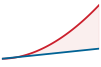
Compute capacity outruns memory bandwidth; the widening gap is the memory wall.
Knowing that these barriers exist is necessary but not sufficient. Given a specific ML workload (say, a recommendation engine or a wake-word detector), we need to determine which paradigm fits and which barrier the workload will hit first. The answer requires analytical tools that connect workload characteristics to these physical constraints: the iron law to decompose latency, the bottleneck principle to identify the dominant constraint, and a set of workload archetypes to classify where each model falls on the spectrum.
Self-Check: Question
A safety-critical autonomous braking system requires an end-to-end decision latency budget of 10 ms. A cloud data center is located 1,500 km away. Given that light travels through optical fiber at approximately \(200{,}000\text{ km/s}\), why is offloading inference to this cloud data center physically impossible?
- The cloud server queue latency always adds at least 25 ms regardless of server load.
- The speed of light in fiber allows a round trip in 5 ms, but serialization of model weights requires 15 ms.
- The minimum speed-of-light round-trip propagation time alone is 15 ms, consuming the entire 10 ms budget before compute begins.
- Wireless transmission protocols require a minimum 50 ms handshake before transmitting sensor packets.
Under dynamic CMOS power scaling where supply voltage scales proportionally with clock frequency (\(V \propto f\)), doubling the processor clock frequency increases dynamic power dissipation by a factor of 8 (\(f^3\)).
How does the memory wall manifest in modern computing hardware according to the historical growth rates of compute capacity versus memory bandwidth?
- Memory bandwidth doubles every 18 months while compute throughput increases by only 20% annually, causing compute starvation.
- Both compute throughput and memory bandwidth grow at identical 60% annual rates, but memory capacity limits model size.
- Processors have reached absolute thermal limits while memory signaling energy has dropped to near-zero levels.
- Compute capacity historically doubles roughly every 18 months (~60% annually), whereas memory bandwidth grows by only ~20% annually, causing the compute-to-bandwidth gap to widen compounding over time.
What causes thermal throttling on passively cooled mobile devices running sustained ML inference, and how does it affect continuous model execution?
The historical scaling relationship under which shrinking MOSFET transistor dimensions allowed reducing voltage and current while keeping power density constant is known as ____ scaling.
Analyzing Workloads
Given a recommendation engine or wake-word detector, the workload question is which term will bind first on the target hardware. The central analytical tool for answering that silicon-contract question is the iron law of ML systems, established in Iron Law of ML Systems. Here, \(T\) is total time, \(D_{\text{vol}}\) is bytes moved, \(\text{BW}\) is bandwidth, \(O\) is total operations, \(R_{\text{peak}}\) is peak compute rate, \(\eta_{\text{hw}}\) is hardware efficiency, and \(L_{\text{lat}}\) is fixed overhead; equation 4 adds these costs for a serialized execution path: \[T = \frac{D_{\text{vol}}}{\text{BW}} + \frac{O}{R_{\text{peak}} \cdot \eta_{\text{hw}}} + L_{\text{lat}} \tag{4}\]
Equation 4 decomposes total latency into three terms: data movement \((D_{\text{vol}}/\text{BW})\), compute \((O/(R_{\text{peak}} \cdot \eta_{\text{hw}}))\), and fixed overhead \((L_{\text{lat}})\). For a single inference, these costs simply add up—each is paid sequentially. In production systems, however, tasks are processed continuously as a stream, and the analysis shifts from single-task latency to identifying which term limits the system. The answer depends entirely on the deployment environment: a model that is compute bound during training may become memory bound during inference; a system that runs efficiently in the cloud may hit power limits on mobile devices. To determine which term dominates, we need a companion principle.
The bottleneck principle
The iron law tells us the cost of each term. The bottleneck principle tells us which term matters. In a pipelined ML workload, identifying the system bottleneck matters because optimizing fast operations yields zero benefit while the slowest stage remains unchanged. Modern accelerators use pipelined execution to overlap data movement with computation: while the accelerator computes on batch \(n\), the memory system prefetches batch \(n+1\). When data movement, computation, and I/O are fully overlapped in steady state, let \(T_{\text{network}}\) denote remote-transfer time and \(T_{\text{bottleneck}}\) the resulting per-task time, including fixed overhead. The faster stages hide behind the slowest overlapped stage, so the iron law’s sum becomes a maximum, as equation 5 formalizes: \[ T_{\text{bottleneck}} = \max\left(\frac{D_{\text{vol}}}{\text{BW}}, \frac{O}{R_{\text{peak}} \cdot \eta_{\text{hw}}}, T_{\text{network}}\right) + L_{\text{lat}} \tag{5}\]
- \(\frac{D_{\text{vol}}}{\text{BW}}\) (Memory): Time to move data between memory and processor.
- \(\frac{O}{R_{\text{peak}} \cdot \eta_{\text{hw}}}\) (Compute): Time to execute calculations.
- \(T_{\text{network}}\): Time for network communication (if offloading).
- \(L_{\text{lat}}\) (Overhead): Fixed latency (kernel launch, runtime overhead).
When a system is memory bound \((D_{\text{vol}}/\text{BW} > O/(R_{\text{peak}} \cdot \eta_{\text{hw}}))\), faster processors \((R_{\text{peak}})\) yield no speedup, just as widening a highway cannot help traffic constrained by a narrow bridge. Engineers must identify the dominant term before optimizing. When network transfer is a candidate term, offloading adds energy to the time-based analysis. The local-versus-offload decision must therefore weigh joules as well as milliseconds.
Napkin Math 1.1: The energy of transmission
Problem: Should a battery-powered sensor process data locally (on-device NPU inference) or send it to the cloud when the energy of transmission collides with the battery-driven energy wall?
Given:
- Data \((D_{\text{vol}})\): 1 MB (illustrative payload volume).
- Transmission energy \((E_{\text{tx}})\): 100 mJ/MB (Wi-Fi/LTE).
- Compute energy \((E_{\text{op}})\): 0.1 mJ/inference (illustrative MobileNetV2 neural-processing-unit anchor).
Math:
- Cloud approach: \(E_{\text{cloud}} \approx D_{\text{vol}} \times E_{\text{tx}}\) = 1 MB \(\times\) 100 mJ/MB = 100 mJ.
- Local approach: \(E_{\text{local}} \approx\) Inference = 0.1 mJ.
Systems insight: Transmitting raw data is 1,000× more expensive than processing it locally. Even if the cloud had infinite speed \((T \approx 0)\), the stated battery budget favors local inference over raw-data transmission. The machine constraint (battery) shapes the deployment choice.
The iron law’s variables interact differently across deployment scenarios. Before specific workload archetypes are examined, these core performance determinants need a compact definition.
Systems Perspective 1.1: The iron law as deployment diagnostic
The iron law introduced in Iron Law of ML Systems is the deployment diagnostic used throughout this chapter: it expresses the total time \(T\) required for a workload as the sum of data movement, arithmetic, and latency: \[T = \frac{D_{\text{vol}}}{\text{BW}} + \frac{O}{R_{\text{peak}} \cdot \eta_{\text{hw}}} + L_{\text{lat}}\] This decomposition is diagnostic: it quantifies how data volume \((D_{\text{vol}})\), compute capacity \((R_{\text{peak}})\), and fixed latency \((L_{\text{lat}})\) jointly set a workload’s time budget. Unlike Amdahl’s Law, which focuses on parallel speedup, the iron law binds model work to data movement and fixed latency at the deployment boundary. The frequent misconception is that these terms are independent; in reality they are trade-off axes. Increasing batch size can improve duty cycle and data reuse, shifting a memory-bound kernel toward compute-bound behavior, while also increasing the working set and batch service time.

The machine axis sets the deployment envelope.
The iron law quantifies the cost of each ingredient; the bottleneck principle identifies the speed of the assembly line. As a rule of thumb, use the additive form in equation 4 when analyzing the latency of a single task, and the max form in equation 5 when analyzing the throughput of a continuous stream of tasks.
Workload archetypes
The bottleneck principle reduces optimization to identifying the dominant constraint for a given workload. The answer depends on the D·A·M taxonomy in The D·A·M Intersection Landscape, which decomposes every ML system into Data, Algorithm, and Machine. Different deployment environments create different bottlenecks along these axes, so the same model family can require different engineering when it moves from a cloud server with terabytes of memory to a microcontroller with kilobytes. The iron law turns that diagnostic into four workload archetypes.5 These are not model categories; they are recurring physical bottlenecks that determine which engineering moves can help.
5 Workload archetype: A classification of ML workloads by their dominant iron law bottleneck rather than their model family. The distinction matters because the optimization strategy differs fundamentally: a compute-bound workload benefits from faster arithmetic \((R_{\text{peak}})\), while a bandwidth-bound workload benefits from wider memory buses or fewer bytes moved through reuse, fusion, compression, or lower precision. Misidentifying the archetype wastes optimization effort on the wrong term of the iron law, as when teams add accelerator FLOP/s to a memory-bound inference pipeline and observe zero speedup.
The first split separates arithmetic-bound systems from data-movement-bound systems. A compute beast performs many calculations per byte loaded, so progress comes from higher arithmetic throughput, better utilization, and more parallel execution; large neural-network training is the canonical case. A bandwidth hog, by contrast, waits on dense weight or activation movement, so wider memory buses and better data reuse matter more than additional peak FLOP/s; autoregressive text generation illustrates this regime.
The second split covers workloads where the binding constraint is not dense arithmetic at all. Sparse scatter workloads are dominated by irregular table lookups and poor cache locality, so memory capacity, access latency, and communication shape performance in recommendation systems with massive embedding tables. Tiny constraint workloads face the opposite envelope: energy per inference and memory footprint, not raw speed, determine whether always-on sensing can run at all.
Lighthouse 1.1: Five reference workloads
The five lighthouse models summarized in table 2 recur throughout this book as concrete workloads that span the deployment spectrum and isolate distinct system bottlenecks. Network Architectures provides full architectural details and model biographies.
| Lighthouse | Archetype | Deployment Paradigm |
|---|---|---|
| ResNet-50 | Compute Beast | Cloud training, edge inference |
| GPT-2/Llama | Bandwidth Hog | Cloud inference |
| DLRM | Sparse Scatter | Cloud only (distributed) |
| MobileNetV2 | Compute Beast (efficient) | Mobile, edge |
| Keyword Spotting (KWS) | Tiny Constraint | TinyML, always-on |
These archetypes map naturally to deployment paradigms. Compute beasts and sparse scatter workloads gravitate toward cloud ML where resources are abundant, bandwidth hogs span cloud and edge depending on latency requirements, and tiny constraint workloads belong to TinyML. Each archetype therefore maps to a specific model that recurs throughout this book as one of five reference workloads.
The five lighthouse models ground the abstract interdependencies of the iron law in concrete practice. These summaries connect each workload to the specific iron law bottleneck it exemplifies.
The first lighthouse, ResNet-50, classifies images into 1,000 categories, processing each image through approximately 8.2 GFLOP using 25.6 million parameters (102.4 MB at FP32) (He et al. 2016). Used in medical imaging diagnostics, autonomous vehicle perception pipelines, and as the backbone for content moderation systems, its regular, compute-dense structure makes it the canonical benchmark for hardware accelerator performance.
He, Kaiming, Xiangyu Zhang, Shaoqing Ren, and Jian Sun. 2016. “Deep Residual Learning for Image Recognition.” 2016 IEEE Conference on Computer Vision and Pattern Recognition (CVPR), 770–78. https://doi.org/10.1109/cvpr.2016.90.
Radford, Alec, Jeffrey Wu, Rewon Child, David Luan, Dario Amodei, and Ilya Sutskever. 2019. Language Models Are Unsupervised Multitask Learners. OpenAI.
Touvron, Hugo, Thibaut Lavril, Gautier Izacard, Xavier Martinet, Marie-Anne Lachaux, Timothée Lacroix, Baptiste Rozière, et al. 2023. “LLaMA: Open and Efficient Foundation Language Models.” arXiv Preprint arXiv:2302.13971.
Pope, Reiner, Sholto Douglas, Aakanksha Chowdhery, Jacob Devlin, James Bradbury, Jonathan Heek, Kefan Xiao, Shivani Agrawal, and Jeff Dean. 2023. “Efficiently Scaling Transformer Inference.” Proceedings of Machine Learning and Systems (MLSys) 5: 606–24.
The language models GPT-2/Llama exemplify autoregressive text generation (Radford et al. 2019; Touvron et al. 2023). These models generate text one token at a time. During low-batch decoding, producing each token may require moving most or all model parameters (1.5 billion parameters for GPT-2, 7 billion–70 billion parameters for Llama) through memory. This sequential access pattern creates an autoregressive bottleneck that shapes serving cost (Pope et al. 2023).
The recommendation lighthouse, DLRM, represents the embedding-heavy recommendation workload behind large-scale “You might also like” systems (Naumov et al. 2019). It maps users and items to embedding vectors stored in tables that can exceed 100 GB of embeddings, making memory capacity rather than computation the binding constraint.
Naumov, Maxim, Dheevatsa Mudigere, Hao-Jun Michael Shi, Jianyu Huang, Narayanan Sundaraman, Jongsoo Park, Xiaodong Wang, et al. 2019. “Deep Learning Recommendation Model for Personalization and Recommendation Systems.” arXiv Preprint arXiv:1906.00091.
Sandler, Mark, Andrew Howard, Menglong Zhu, Andrey Zhmoginov, and Liang-Chieh Chen. 2018. “MobileNetV2: Inverted Residuals and Linear Bottlenecks.” 2018 IEEE/CVF Conference on Computer Vision and Pattern Recognition, 4510–20. https://doi.org/10.1109/cvpr.2018.00474.
The mobile lighthouse, MobileNetV2, is designed for efficient mobile vision tasks such as classification, detection, and segmentation (Sandler et al. 2018). It performs the same image classification task as ResNet but uses depthwise separable convolutions, which separate spatial filtering from channel mixing, to reduce computation by 13.7×, enabling real-time inference on smartphones at 3–5 W.
The TinyML lighthouse, keyword spotting (KWS), represents the always-on sensing archetype. KWS systems detect short trigger phrases with compact models built for resource-constrained microcontrollers (Zhang et al. 2017); in the Smart Doorbell scenario, that same pattern becomes a local “Ding Dong” or “Hello” trigger. The lighthouse workload has approximately 200K parameters and fits in about 800 KB, placing it in the kilobyte-memory, milliwatt-budget TinyML regime.
Zhang, Yundong, Naveen Suda, Liangzhen Lai, and Vikas Chandra. 2017. Hello Edge: Keyword Spotting on Microcontrollers.
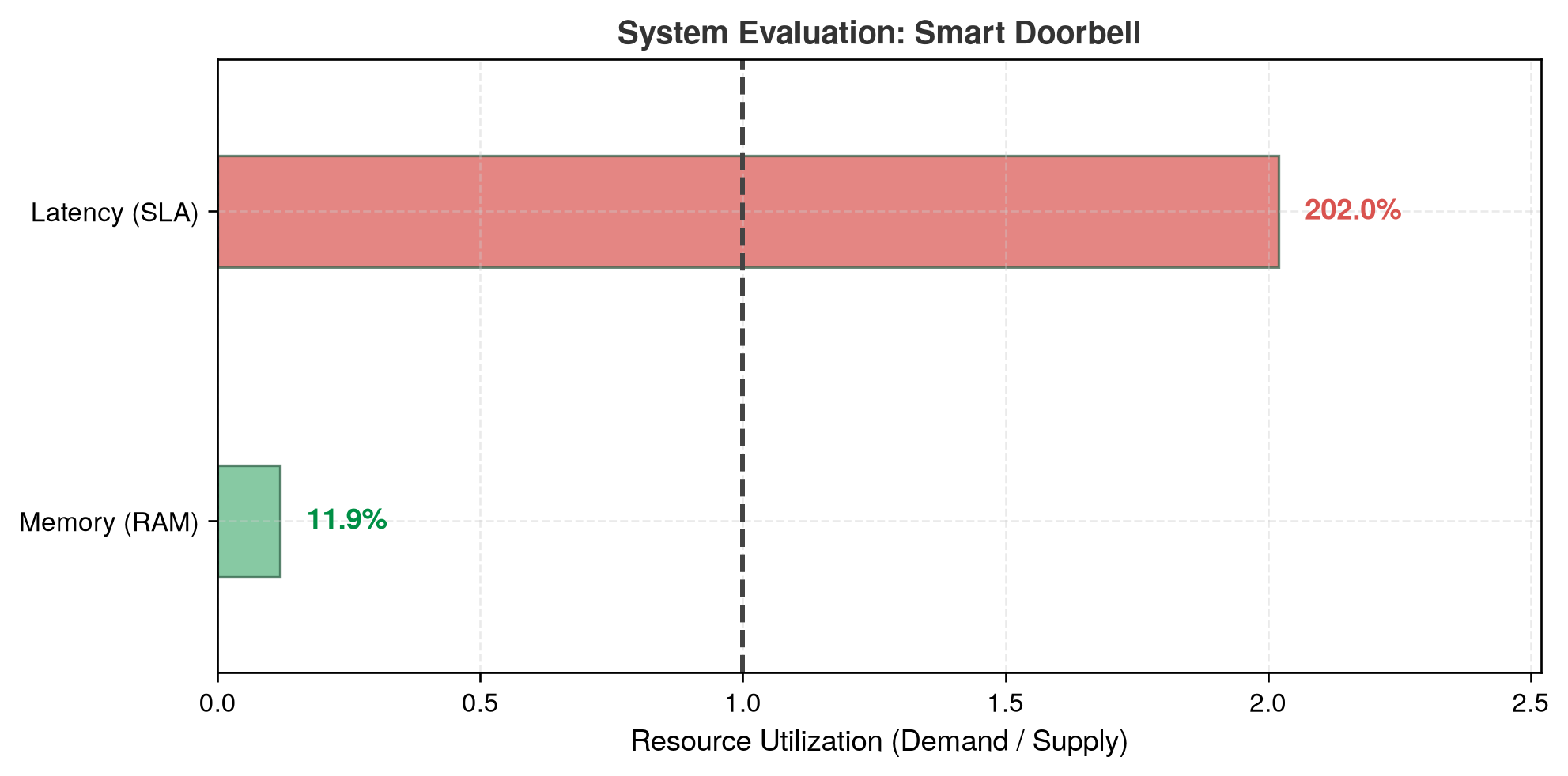
Deployment feasibility is evaluated hierarchically, verifying physical memory fit before checking execution latency. In figure 2, horizontal bars plot resource demand as a percentage of supply against the vertical 100 percent saturation threshold for the ESP32-S3 microcontroller, comparing Level 1 memory capacity with Level 2 latency under the service level agreement (SLA).
The range in compute requirements and memory footprints explains why no single deployment paradigm fits all workloads. A keyword spotter can operate with roughly 20 MFLOP and 800 KB, while ResNet-50 requires about 8.2 GFLOP and roughly 102.4 MB per image. The reference DLRM example already reaches 100 GB, and production DLRM-style recommendation systems can exceed 100 TB. Language models add a bandwidth-dominated regime: billions of parameters streamed repeatedly from memory during autoregressive inference. These five lighthouse models serve as concrete anchors throughout the book, each isolating a distinct system bottleneck revisited in every chapter.
Analytical tools alone remain abstract until grounded in real silicon. The next step translates the iron law, bottleneck principle, and workload archetypes into quantitative engineering decisions by examining how system balance (the interplay of compute, memory, and I/O) varies across real hardware platforms.
Self-Check: Question
When analyzing ML system performance, when should an engineer apply the additive form of the iron law (\(T = \frac{D_{\text{vol}}}{\text{BW}} + \frac{O}{R_{\text{peak}} \cdot \eta_{\text{hw}}} + L_{\text{lat}}\)) versus the bottleneck principle’s max form (\(T = \max\left(\frac{D_{\text{vol}}}{\text{BW}}, \frac{O}{R_{\text{peak}} \cdot \eta_{\text{hw}}}, T_{\text{network}}\right) + L_{\text{lat}}\))?
- Use the additive form for single-task, serialized latency, and the max form for pipelined, steady-state throughput where computation and data prefetching overlap.
- Use the additive form exclusively for cloud workloads, and the max form exclusively for microcontroller TinyML workloads.
- Use the additive form when batch size is greater than 128, and the max form when batch size equals 1.
- Use the additive form during model training only, and the max form during on-device model quantization.
Which pairing correctly matches a workload archetype to its dominant physical bottleneck and canonical lighthouse model?
- Compute Beast \(\rightarrow\) dominated by irregular table lookups and cache misses \(\rightarrow\) DLRM
- Bandwidth Hog \(\rightarrow\) dominated by dense parameter streaming during autoregressive token decode \(\rightarrow\) GPT-2/Llama
- Sparse Scatter \(\rightarrow\) dominated by dense FLOP throughput at high arithmetic intensity \(\rightarrow\) ResNet-50
- Tiny Constraint \(\rightarrow\) dominated by petabyte-scale distributed training \(\rightarrow\) Keyword Spotting (KWS)
In a battery-powered IoT sensor, why does sending raw sensor data (e.g., 1 MB audio) over a cellular or Wi-Fi radio often consume significantly more energy than running local neural network inference (e.g., MobileNetV2)?
Order the steps of the hierarchical deployment feasibility evaluation for the Smart Doorbell scenario from initial resource check to latency verification:
- Verify Level 1 resource capacity fit (confirm model weights and activations fit in microcontroller SRAM/Flash)
- Define application mission targets (specify model task, accuracy target, and real-time SLA budget)
- Verify Level 2 timing constraints (evaluate per-inference execution latency against the strict interaction SLA)
- Select deployment candidate platform and model archetype (match keyword spotter to ESP32-S3 microcontroller)
- An ML workload characterized by high arithmetic intensity where throughput is bounded by peak FLOP/s (\(R_{\text{peak}}\)) rather than memory bandwidth, such as dense convolutional neural network training, belongs to the ____ archetype.
System Balance and Hardware
Physical constraints translate latency-vs-throughput trade-offs into engineering decisions through concrete numbers. Table 3 provides order-of-magnitude latencies that should inform every deployment decision—spanning eight orders of magnitude from nanosecond compute operations to hundreds of milliseconds for cross-region network calls. Detailed hardware latencies and bandwidth constraints are covered in Hardware Acceleration. An operation with latency \(> X\) cannot appear on the critical path of a system whose latency budget is \(X\) ms.6
6 Critical path: The longest sequential chain of dependent operations in a pipeline. The decision rule in the triggering sentence is strict: if a 200 ms cross-region network call appears anywhere on the critical path, a system with a 100 ms total budget is guaranteed to fail regardless of how fast every other stage runs. Model inference need not be the longest stage; preprocessing and postprocessing can dominate, making the critical path longer than model execution alone suggests.
| Operation | Latency | Deployment Implication |
|---|---|---|
| Compute | ||
| GPU matrix multiply (per op) | ~1 ns | Per-operation latency is small |
| NPU inference (MobileNetV2) | 5–20 ms | Mobile can do real-time vision |
| LLM token generation | 20–100 ms | Perceived as “typing speed” |
| Memory | ||
| L1 cache hit | ~1 ns | Keep hot data in registers |
| Uncached GPU memory read | ~200–500 ns | Hide latency; coalesce accesses |
| DRAM read (mobile) | 50–100 ns | Repeated reads can limit workloads |
| Network | ||
| Same data center | 0.5 ms | Microservices feasible |
| Same region | 1–5 ms | Edge servers viable |
| Cross-region | 50–150 ms | Poor fit for tight latency budgets |
| ML Operations | ||
| Wake-word detection (TinyML) | ~1–10 ms | Always-on feasible at \(<1\text{ mW}\) |
| Face detection (mobile) | 10–30 ms | Real-time at 30 FPS |
| GPT-4 first token | 200–500 ms | User notices delay |
| ResNet-50 training step | 200–400 ms | Throughput-optimized |
The four deployment paradigms gain precision when grounded in concrete hardware. While table 1 defined the paradigms conceptually, table 6 provides specific devices, processors, and quantitative thresholds for selecting deployment targets.7 The same nine-order power span, coupled with data center power usage effectiveness (PUE) metrics,8 joins a cost spread from $millions to $10 to determine which paradigm serves a given workload economically.
7 ML hardware cost spectrum: AI infrastructure spans six orders of magnitude in cost, from $10 microcontrollers to multi-million-dollar accelerator clusters. This million-fold range means deployment paradigm selection is simultaneously a physics decision and an economics decision. Even within individual-device choices, the same accuracy target may be achievable on a low-cost microcontroller only after substantial model reduction, or on an expensive data-center accelerator with a much larger resource budget, with fundamentally different latency, power, and operational cost profiles.
8 Power usage effectiveness (PUE): This metric isolates facility energy overhead, including cooling and power distribution, from the energy delivered to computing equipment. Even a PUE of 1.06 leaves substantial noncompute power at data-center scale. TinyML does not require dedicated facility cooling, although sensing, communication, conversion losses, and sleep power still contribute to its complete system-energy budget. These device-level costs sit outside PUE.
These hardware differences translate directly into performance bottlenecks. To understand which constraint dominates in each paradigm, we apply the bottleneck principle (section 1.2.1).
Systems Perspective 1.2: System balance across paradigms
The pipelined form of the iron law of ML systems from Iron Law of ML Systems adds \(\text{BW}_{\text{IO}}\), the storage or network I/O bandwidth, to the canonical compute and memory terms. Equation 6 formalizes the resulting lower bound on total execution time \(T\): \[T \geq \max\left( \frac{O}{R_{\text{peak}} \cdot \eta_{\text{hw}}}, \frac{D_{\text{vol}}}{\text{BW}}, \frac{D_{\text{vol}}}{\text{BW}_{\text{IO}}} \right) + L_{\text{lat}} \tag{6}\]
Here, \(O\) represents total operations, \(R_{\text{peak}}\) is peak compute rate, \(\eta_{\text{hw}}\) is hardware utilization efficiency, \(D_{\text{vol}}\) is data volume, \(\text{BW}\) is memory bandwidth, \(\text{BW}_{\text{IO}}\) is I/O bandwidth (storage or network), and \(L_{\text{lat}}\) is fixed overhead. The lower bound identifies which resource (compute, memory, or I/O) limits performance; equality requires ideal overlap with no additional stalls. The dominant term varies by workload and deployment regime. Faster accelerators help compute-bound cloud training; memory-bound large language model (LLM) decode and edge workloads benefit more from reducing bytes moved or increasing bandwidth. Table 4 works through all four paradigms, splitting cloud into training and LLM inference, and Bottleneck diagnostic maps each dominant term to the optimizations that work and the ones that are wasted, turning this diagnosis into an action plan.
| Paradigm | Dominant Constraint | Why | Optimization Focus |
|---|---|---|---|
| Cloud Training | \(O/(R_{\text{peak}} \cdot \eta_{\text{hw}})\) (Compute) | Abundant memory/network; FLOP/s limit throughput | Maximize accelerator utilization, batch size |
| Cloud LLM Inference | \(D_{\text{vol}}/\text{BW}\) (memory bandwidth) | Sequential generation repeatedly moves model state | Increase reuse; reduce bytes moved |
| Edge Inference | \(D_{\text{vol}}/\text{BW}\) (memory bandwidth) | Limited local bandwidth; models often memory-bound | Smaller models; fewer memory transfers |
| Mobile | Energy (implicit) | Battery = \(\int \text{Power} \cdot dt\); thermal throttling | Lower precision; duty cycling |
| TinyML | Model footprint must fit on-chip (capacity) | Kilobyte-scale memory; model must fit on-chip | Tiny models and fixed-point arithmetic |
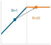
Batch-1 inference sits on the memory-bound side of the roofline.
Williams, Samuel, Andrew Waterman, and David Patterson. 2009. “Roofline: An Insightful Visual Performance Model for Multicore Architectures.” Communications of the ACM 52 (4): 65–76. https://doi.org/10.1145/1498765.1498785.
Roofline analysis classifies bottlenecks by comparing a workload’s arithmetic intensity—the ratio of floating-point operations performed per byte of memory moved (\(\text{FLOPs/byte}\))—against the hardware machine balance point (\(R_{\text{peak}} / \text{BW}\)) (Williams et al. 2009). The framing is informal here; The Roofline model derives the model in full, defining arithmetic intensity formally and deriving the ridge point that separates the memory-bound and compute-bound regimes. In that framing, the same ResNet-50 model can shift from compute-bound training behavior at high batch sizes to more memory-sensitive single-image inference at batch=1. Deployment paradigm selection must account for this shift.
This shift between training and inference is critical to understand. Recall the D·A·M taxonomy from The D·A·M Intersection Landscape: every ML system comprises Data, Algorithm, and Machine. Table 5 shows how each component behaves differently depending on whether the system is training (learning patterns) or serving (applying them).
| Component | Training (Mutable) | Inference (Immutable) |
|---|---|---|
| Data | Massive throughput: large batches, shuffling, augmentation | Low latency: single samples, freshness, speed |
| Algorithm | Learning phase: update model parameters from examples | Prediction phase: apply fixed weights to new inputs |
| Machine | Throughput-optimized: high-bandwidth clusters, large memory | Latency-optimized: edge devices, inference accelerators |
A quantitative comparison applies this analysis to ResNet-50 inference on a high-end data center accelerator and a mobile NPU. Treat these as point-in-time hardware anchors: the arithmetic is about compute rate, memory bandwidth, and batch size, while Hardware Acceleration explains the accelerator architecture behind the numbers.
Napkin Math 1.2: ResNet-50 on cloud vs. mobile
Problem: Is ResNet-50 inference compute bound or memory bound on (a) a high-end data center accelerator and (b) a flagship mobile NPU?
Given (from lighthouse models):
- ResNet-50: 8.2 GFLOP per inference, 25.6 million parameters (102.4 MB FP32, 51.2 MB FP16)
Analysis:
(a) Cloud data-center accelerator (batch=1, FP16)
- Peak compute: 312 TFLOP/s (FP16)
- Memory bandwidth: 2.04 TB/s
- Compute time: \(T_{\text{comp}}\) = \(\frac{8.20 \times 10^{9}}{3.12 \times 10^{14}}\) = 0.026 ms
- Memory time (weights plus activations): \(T_{\text{mem}}\) = \(\frac{5.63 \times 10^{7}}{2.04 \times 10^{12}}\) = 0.028 ms
- Result: Bottleneck = Memory (1.1× slower than compute)
- Analysis: Compute per byte moved = \(\frac{8.20 \times 10^{9}}{5.63 \times 10^{7}}\) = 146 FLOP/byte. This ratio measures how much arithmetic the workload performs for each byte loaded. When the ratio exceeds the hardware’s compute-to-bandwidth ratio \((R_{\text{peak}}/\text{BW})\), the workload is compute bound; below it, the workload is memory bound. For single-image inference, the low batch size yields limited reuse, explaining why even powerful accelerators can be memory bound at batch = 1.
(b) Mobile: Flagship NPU (batch=1, INT8)
- Peak compute: ~35 TOPS (INT8)—representative of modern mobile NPUs
- Memory bandwidth: ~51.2 GB/s (LPDDR5)
- Model size: 25.6 MB (INT8 quantized)
- Compute time: \(T_{\text{comp}}\) = \(\frac{8.20 \times 10^{9} \text{ INT8 ops}}{3.50 \times 10^{13} \text{ INT8 ops/s}}\) = 0.23 ms
- Memory time (weights plus activations): \(T_{\text{mem}}\) = \(\frac{2.82 \times 10^{7}}{5.12 \times 10^{10}}\) = 0.55 ms
- Result: Bottleneck = Memory (2.3× slower than compute)
Systems insight: Both platforms are memory bound for single-image inference. The A100’s faster memory bandwidth (2.04 TB/s vs. 51.2 GB/s = 39.8×) translates to roughly 19.9× faster inference; peak compute alone is not the limiting comparison. This explains why byte-reduction and lower-precision techniques can beat simply buying more peak FLOP/s for deployment.
ResNet-50 becomes compute bound when batching and data reuse raise computation per byte moved above the hardware balance point, \(I > R_{\text{peak}}/\text{BW}\), where \(I = O/D_{\text{vol}}\). The crossover is architecture- and implementation-dependent because activation traffic, input/output movement, cache reuse, and runtime execution details all change the effective bytes moved per inference.
Compression matters more, not less, as the hardware budget tightens. As systems transition from Cloud to Edge to TinyML, available resources decrease dramatically. Table 6 quantifies this progression with concrete hardware examples: memory drops from 128 TB (cloud) to 512 KB (TinyML), a 250 million-fold reduction, alongside the same megawatt-to-milliwatt power span. This resource disparity is most acute on microcontrollers, the primary hardware platform for TinyML, where memory and storage capacities are insufficient for conventional ML models.
| Category | Example Device | Processor | Memory | Storage | Power | Price Range |
|---|---|---|---|---|---|---|
| Cloud ML | Google TPU v4 Pod | 4,096 TPU v4 chips, 1.1 EFLOP/s BF16 | 128 TB HBM2 | Cloud-scale (PB) | ~3 MW | Cloud service (rental) |
| Edge ML | NVIDIA DGX Spark | GB10 Grace Blackwell, 1 PFLOP/s sparse FP4 | 128 GB LPDDR5x | 4 TB NVMe | ~200 W | ~$3,000–$5,000 |
| Mobile ML | Flagship Smartphone | Mobile SoC (CPU + GPU + NPU) | 8–16 GB | 128 GB-1 TB | 3–5 W | $999+ |
| TinyML | ESP32-S3 | Dual-core @ 240 MHz | 512 KB SRAM | 4 MB Flash | 0.05 W–1.2 W active board power | $10 |
The hardware spectrum turns that bottleneck diagnosis into a fit test. The platforms in table 6 are products of decades of hardware evolution, from floating-point coprocessors in the 1980s through graphics processors in the 2000s to today’s domain-specific AI accelerators. Hardware Acceleration traces this historical progression and the architectural principles that drove it. Here, the consequence matters most: qualitatively different hardware appears at different points in the infrastructure, so each workload must be matched to the region whose compute, memory, power, and cost envelope it can satisfy.
Each paradigm occupies a distinct region of the deployment spectrum, governed by the physical constraints (light barrier, power wall, memory wall) and quantified by the analytical tools (iron law, bottleneck principle) introduced in section 1.2. The quantitative thresholds in table 7 help practitioners determine whether a workload fits a target’s compute, bandwidth, power, and latency envelope.
| Paradigm | Compute | Memory bandwidth | Power | Latency (ms) |
|---|---|---|---|---|
| Cloud ML | > 1000 TFLOP/s | > 1000 GB/s | MW class (PUE 1.1–1.3) | 100-500 |
| Edge ML | ~1 PFLOP/s | > 270 GB/s | 100 W class | 10-100 |
| Mobile ML | 15–45 TOPS | 51.2–77 GB/s | 3–5 W | 5-50 |
| TinyML | < 1 TOPS | — | < 1 mW always-on average target | 1-10 |
Table 7 completes the fit test: each paradigm in the table is an operating envelope with a different binding resource. The next four sections progress from cloud to TinyML, tracing the gradient from maximum computational resources to maximum efficiency constraints while keeping the same questions in view: which term binds, what optimization helps, and which trade-offs follow.
Self-Check: Question
Why is single-image (batch=1) ResNet-50 inference memory-bound on both a high-end cloud accelerator (NVIDIA A100) and a mobile NPU (iPhone 15 Pro)?
- ResNet-50 contains dynamic control flow that causes branching stalls on SIMD execution units.
- Both platforms lack matrix multiplication coprocessors, forcing scalar CPU execution.
- At batch=1, model weights must be loaded from memory once per single image without weight reuse across batch items, keeping arithmetic intensity below each platform’s hardware balance point (\(R_{\text{peak}}/\text{BW}\)).
- The activations at batch=1 exceed the total high-bandwidth memory (HBM) and SRAM capacities of both devices.
Why does a convolutional neural network (e.g., ResNet-50) shift from a compute-bound regime during cloud training to a memory-bound regime during single-sample (\(\text{batch}=1\)) edge inference?
An ML service SLA guarantees a total end-to-end response time of 100 ms. The pipeline involves client preprocessing, a cross-region network RPC, model inference, and postprocessing. According to critical path latency principles, why will this system fail if a cross-region network call taking 120 ms is placed on the synchronous critical path?
- The ML framework compiler will refuse to lower the graph if network RPC operations are detected.
- Cross-region RPCs corrupt the numerical precision of FP16 tensors during serialization.
- A cross-region network call reduces the accelerator compute throughput (\(R_{\text{peak}}\)) by half.
- The critical path is the longest sequential chain of dependent operations; any single stage exceeding 100 ms guarantees the end-to-end SLA will be breached regardless of how fast all other stages execute.
What is the hardware balance point (or roofline ridge point) of an accelerator, and what does it tell an ML systems engineer about whether a workload will be compute-bound or memory-bound?
In ML accelerator memory hierarchies, an L1 cache hit requires approximately 1 ns, whereas an uncached global DRAM read requires approximately 200–____ ns.
Cloud ML: Computational Power
Consider what it took to train GPT-3:9 3,634.3 PFLOP-days of computation, 10,000 V100 GPUs running for approximately 15 days, consuming megawatts of power (Patterson et al. 2021). No smartphone, edge server, or single machine could have completed this training run on a practical schedule. It required a data-center-scale cluster with enough aggregate compute, memory, and storage. This is the defining proposition of cloud ML: when latency can be tolerated, it offers computational scale that no other paradigm can match.
9 Large language model (LLM) training scale: GPT-3 required approximately 3,634.3 PFLOP-days (Patterson et al. 2021). This scale illustrates the core cloud ML trade-off: only centralized infrastructure can aggregate enough \(R_{\text{peak}}\) for large training runs, but remote inference adds network latency and is unsuitable when the end-to-end path exceeds the application’s latency budget.
Patterson, David, Joseph Gonzalez, Quoc Le, Chen Liang, Lluis-Miquel Munguia, Daniel Rothchild, David So, Maud Texier, and Jeff Dean. 2021. “Carbon Emissions and Large Neural Network Training.” arXiv Preprint arXiv:2104.10350.
10 Cloud as utility computing: The utility model allows providers to offer a specialized hardware portfolio that is economically infeasible for a single organization to maintain. This provides direct, on-demand access to the specific architectures required by each workload archetype: dense accelerator pods for Compute Beasts, HBM-equipped nodes for Bandwidth Hogs, and high-memory systems with fast interconnects for Sparse Scatter. A team can therefore rent a purpose-built, $10M+ supercomputing pod for a few hours rather than owning it.
Cloud ML aggregates computational resources in data centers10 to handle computationally intensive tasks: large-scale data processing, collaborative model development, and advanced analytics. This infrastructure serves as the natural home for three of the four workload archetypes: Compute Beast workloads like ResNet training that demand sustained TFLOP/s across thousands of accelerators, Bandwidth Hog workloads like large language model inference that benefit from TB/s HBM bandwidth, and Sparse Scatter workloads like recommendation systems that require terabytes of embedding tables and high-bandwidth interconnects for all-to-all communication patterns.
Cloud deployments range from single-machine instances (workstations, multi-GPU servers, DGX systems) to large-scale distributed systems spanning multiple data centers. This book focuses on single-machine cloud systems, where the reader learns to build and optimize ML systems on individual powerful machines. Future studies can address distributed cloud infrastructure, where systems coordinate computation across multiple networked machines. This follows the principle of establishing foundations before adding complexity.
Cloud deployment offers elastic compute while adding distance to remote paths.
Definition 1.1: Cloud ML
Cloud machine learning is the deployment paradigm that trades latency for elastic compute by locating ML workloads in centralized data centers, decoupling computational capacity from the physical location of data sources and users.
- Significance: Cloud deployment dominates the \(R_{\text{peak}}\) term: a single cloud region can provision thousands of accelerators on demand, delivering aggregate throughput that no typical on-premise installation can match economically. The trade-off is the \(L_{\text{lat}}\) term: a minimum round-trip latency of 10–100 ms (set by the speed of light over continental distances) makes cloud infeasible for any workload requiring sub-10 ms response.
- Distinction: Unlike edge ML, which prioritizes latency determinism and data locality at fixed \(R_{\text{peak}}\), cloud ML prioritizes elastic \(R_{\text{peak}}\) at the cost of variable \(L_{\text{lat}}\).
- Common pitfall: A frequent misconception is that cloud ML is “unlimited compute.” In reality, the distance penalty \((L_{\text{lat}})\) and the ingestion bottleneck \((D_{\text{vol}}/\text{BW})\) are physics constraints that no software optimization can eliminate, setting a hard floor on response time for any workload whose data originates outside the data center.
Centralization defines the cloud bargain: pooling elastic compute across warehouse-scale clusters eliminates local capacity limits, but introduces distance and network latency. The four-column tree in figure 3 maps this trade-off from left to right, connecting the binding scale constraint to its system response, failure boundaries, and well-matched workloads. The examples that thrive in this regime, including virtual assistants, recommendation systems, and fraud detection, all tolerate that bargain because scale matters more than immediacy. The most fundamental challenge, network latency, is not an engineering limitation but a physics constraint. A quick calculation of the distance penalty makes this concrete.
Napkin Math 1.3: The distance penalty
Problem: Consider a real-time safety monitor for a robotic arm. The safety logic requires a 10 ms end-to-end response time to prevent injury, so the distance penalty imposed by the light barrier matters. The model runs in a high-performance cloud data center 1,500 km away. Can the safety budget be met?
Physics:
- Light in fiber: ~200,000 km/s.
- Round-trip propagation: (1,500 km \(\times\) 2)/200,000 km/s = 15 ms.
- Result: Round-trip propagation alone requires 15 ms, exceeding the 10 ms end-to-end budget (-5 ms headroom) before the model performs any inference.
Systems insight: Physics has made cloud ML impossible for this application. The model must move to the Edge.
\begin{tikzpicture}[font=\small\sffamily]
\tikzset{
  Box/.style={inner xsep=2pt,
  draw=GreenLine,
  fill=GreenL!50,
  node distance=0.3,
    line width=0.75pt,
    anchor=west,
    text width=30mm,align=flush center,
    minimum width=30mm, minimum height=10.0mm
  },
  Box2/.style={Box,draw=BlueLine,fill=BlueL!50, text width=32mm, minimum width=31mm
  },
  Box3/.style={Box,draw=OrangeLine,fill=OrangeL!40, text width=30mm, minimum width=32mm
  },
 Box4/.style={Box,draw=VioletLine,fill=VioletL2!40, text width=32mm, minimum width=32mm
  },
 Line/.style={line width=1.0pt,black!50,text=black,-{Triangle[width=0.8*6pt,length=0.98*6pt]}},
}
\node[Box4, fill=VioletL2!90!violet!50,](B1){Binding\\ Constraint};
\node[Box2,right=2 of B1,fill=BlueL](B2){System\\ Response};
\node[Box,right=2 of B2,fill=GreenL](B3){Failure\\ Boundary};
\node[Box3,right=2 of B3,fill=OrangeL](B4){Workloads\\ That Fit};
\node[Box,draw=OliveLine,fill=OliveL!30, minimum height=11.5mm,
above=0.5 of $(B2.north east)!0.5!(B3.north west)$](B0){Cloud ML};
%
\node[Box4,below=0.5 of B1](B11){Scale Exceeds\\ Local Machines};
\node[Box4,below=of B11](B12){Data or State\\ Is Centralized};
\node[Box4,below=of B12](B13){Latency Budget\\ Is Relaxed};
\node[Box4,below=of B13](B14){Usage Is\\ Elastic};
%
\node[Box2,below=0.5 of B2](B21){Pool Accelerators\\ and Storage};
\node[Box2,below=of B21](B22){Shard Data\\ and Models};
\node[Box2,below=of B22](B23){Schedule at\\ Fleet Scale};
\node[Box2,below=of B23](B24){Centralize\\ Operations};
%
\node[Box,below=0.5 of B3](B31){Speed-of-Light\\ Latency};
\node[Box,below=of B31](B32){Internet\\ Dependence};
\node[Box,below=of B32](B33){Data Sovereignty\\ Exposure};
\node[Box,below=of B33](B34){Utilization-Driven\\ Cost};
%
\node[Box3,below=0.5 of B4](B41){Large-Model\\ Training};
\node[Box3,below=of B41](B42){Recommendation\\ Systems};
\node[Box3,below=of B42](B43){Fraud\\ Detection};
\node[Box3,below=of B43](B44){Cloud-Assisted\\ Voice};
%
\foreach \i in{1,2,3,4}{
  \foreach \x in{1,2,3,4}{
\draw[Line](B\x.west)--++(180:0.5)|-(B\x\i);
}
}
\foreach \x in{1,2,3,4}{
\draw[Line](B0)-|(B\x);
}
\end{tikzpicture}Cloud infrastructure and scale
Cloud ML aggregates computational resources in data centers at unprecedented scale. Figure 4 captures the physical scale behind this abstraction: a cloud TPU11 data center floor. TPU supercomputer designs organize thousands of specialized accelerator chips into data-center-scale systems that deliver PFLOP/s-to-EFLOP/s reduced-precision throughput (Jouppi et al. 2023). Table 6 quantifies how cloud systems provide orders-of-magnitude more compute and memory bandwidth than mobile devices, at correspondingly higher power and operational cost. These facilities enable workloads that are impractical on resource-constrained devices, but their remote location introduces critical trade-offs, examined next: network round-trip latency rules out real-time applications, and operational costs scale linearly with usage.
11 Tensor processing unit (TPU): An application-specific integrated circuit (ASIC) that delivers PFLOP/s-scale throughput by hard-wiring its architecture for the matrix multiplication operations that dominate ML workloads. This extreme specialization trades general-purpose flexibility for a \(>10\times\) improvement in performance-per-watt compared to a general-purpose accelerator on the same ML task. The high cost of deploying these accelerators at data center scale is therefore only economical for massive, sustained ML computation.
Jouppi, Norm, George Kurian, Sheng Li, Peter Ma, Rahul Nagarajan, Lifeng Nai, Nishant Patil, et al. 2023. “TPU v4: An Optically Reconfigurable Supercomputer for Machine Learning with Hardware Support for Embeddings.” Proceedings of the 50th Annual International Symposium on Computer Architecture, 1–14. https://doi.org/10.1145/3579371.3589350.
The physical reality of PFLOP/s-scale compute is visible in the infrastructure itself: a single facility floor houses thousands of accelerator chips organized into rows of liquid-cooled racks, each rack consuming kilowatts of power to sustain the aggregate throughput that no individual device can approach.
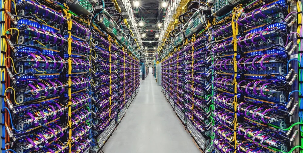
Pichai, Sundar. 2023. Introducing Gemini: Our Largest and Most Capable AI Model.
Cloud ML excels at processing massive data volumes through parallelized architectures, enabling training on datasets requiring hundreds of terabytes of storage and PFLOPs of computation, resources that remain impractical on constrained devices. The training techniques covered in Model Training and the hardware analysis in Hardware Acceleration explain how practitioners achieve this scale.
The same centralization changes how models are shared and operated. Cloud APIs make trained models accessible worldwide across mobile, web, and IoT platforms. Shared infrastructure enables teams to collaborate with integrated version control, while pay-as-you-go pricing models12 replace much infrastructure purchasing with usage-based operating expense and scale with demand.
12 Pay-as-you-go pricing: A cloud economic model where users pay for accelerator-hours consumed rather than hardware owned. Elastic pricing converts the fixed cost of idle \(R_{\text{peak}}\) into a variable cost proportional to actual utilization, but sustained 24/7 workloads can cost more on cloud than equivalent on-premises hardware amortized over three years, a crossover that drives the total cost of ownership (TCO) analysis in table 8.
A common misconception holds that cloud ML’s vast computational resources make it universally superior. Exceptional computational power and storage do not automatically translate to optimal solutions for all applications. The data gravity invariant in Napkin math: The physics of data gravity explains why: as data volume scales, the cost of moving it to compute \((C_{\text{move}}(D_{\text{vol}}) \gg C_{\text{move}}(\text{Compute}))\) eventually dominates. The trade-offs listed in figure 3 become concrete when we consider where edge and embedded deployments excel: real-time response with sub-10 ms decision-making in autonomous control loops, strict data privacy for medical devices processing patient data, predictable costs through one-time hardware investment vs. recurring cloud fees, or operation in disconnected environments such as industrial equipment in remote locations. The optimal deployment paradigm depends on specific application requirements rather than raw computational capability.
Cloud ML trade-offs and constraints
Cloud ML’s advantages carry inherent trade-offs that shape deployment decisions. Latency is the most consequential: remote network latency makes cloud processing unsuitable when the end-to-end path exceeds an application’s response budget. Unpredictable response times further complicate performance monitoring and debugging across geographically distributed infrastructure.
Privacy and security pose serious challenges for cloud deployment. Transmitting sensitive data to remote data centers expands the disclosure surface and complicates regulatory compliance. Organizations handling data subject to regulations such as the General Data Protection Regulation (GDPR)13 or the Health Insurance Portability and Accountability Act (HIPAA)14 must select, document, and maintain safeguards appropriate to the data, system, and applicable legal duties. Privacy-preserving approaches can reduce how much sensitive data must leave its original environment, but they complement rather than replace these controls.
13 GDPR (General Data Protection Regulation): Article 17 provides a right to erasure when specified grounds apply (European Parliament and Council of the European Union 2016). For an ML system, an erasure request requires tracing where the person’s data persists across source stores, derived features, logs, caches, and model artifacts. Retraining may be one remediation, but the regulation does not prescribe retraining every model that encountered the data.
European Parliament, and Council of the European Union. 2016. Regulation (EU) 2016/679 of the European Parliament and of the Council of 27 April 2016. Official Journal of the European Union.
14 HIPAA: The Security Rule requires regulated entities to implement reasonable and appropriate administrative, physical, and technical safeguards for electronic protected health information, including access and audit controls (U.S. Department of Health and Human Services 2005). The rule is technology-neutral and does not mandate confidential-computing enclaves; concrete controls and their performance overhead depend on the system’s risk analysis and implementation.
U.S. Department of Health and Human Services. 2005. “Summary of the HIPAA Security Rule.”
15 Total cost of ownership (TCO): Quantifies the gap between sticker price and true system cost by including all direct and indirect costs (power, cooling, labor) over a system’s lifetime, trading upfront capital expense (CapEx) against recurring operational expense (OpEx). For an on-premise GPU, the purchase price is only one component of the three-year TCO, alongside operating costs.
Cost management introduces operational complexity requiring TCO15 analysis rather than naive unit comparisons. A worked cloud vs. edge TCO comparison illustrates the gap between sticker price and true system cost.
For the worked comparison, table 8 itemizes the annual GPU, network, load-balancer, and observability costs of an illustrative cloud implementation under public list pricing, and table 9 itemizes the corresponding hardware, power, cooling, network, and DevOps labor costs of an on-premise edge-server implementation.
| Cost Component | Calculation | Annual Cost |
|---|---|---|
| GPU inference (A10G) | 4 instances \(\times\) 8760 h/year \(\times\) $0.75/hr | ~$26,280 |
| Network egress | 100 GB/day \(\times\) 365 d/year \(\times\) $0.09/GB | ~$3,285 |
| Load balancer | $0.025/hr + LCU charges | ~$3,723 |
| CloudWatch/logging | Monitoring, alerts | ~$2,000 |
| Total Cloud | ~$35,288/year |
Cloud deployments also carry operational constraints. Unpredictable usage spikes complicate budgeting, requiring comprehensive monitoring and cost governance frameworks. Network dependency creates a further constraint: any connectivity disruption directly impacts system availability, particularly where network access is limited or unreliable. Vendor lock-in compounds this problem, as dependencies on specific tools and APIs create portability challenges when transitioning between providers. Organizations must balance these constraints against cloud benefits based on their specific application requirements and risk tolerance. Even with these constraints, cloud ML is well suited to consumer applications that require elastic capacity at global scale.
| Cost Component | Calculation | Annual Cost |
|---|---|---|
| Hardware CapEx | $15,000 ÷ 3 years life | ~$5,000 |
| Power (24/7) | 300 W \(\times\) 8760 h/year \(\times\) $0.12/kWh | ~$315.4 |
| Cooling overhead | ~30% of power | ~$94.6 |
| Network (fiber) | Fixed line for remote management | ~$1,200 |
| DevOps labor | 0.1 FTE \(\times\) $150,000 salary | ~$15,000 |
| Total Edge | ~$21,610/year |
Napkin Math 1.4: Cloud vs. edge TCO
Problem: A vision system serves 1M daily inferences at ResNet-50 scale (10 ms latency, 100 KB response). When all costs are included (GPU hours, network egress, power, cooling, and labor, itemized in table 8 and table 9), is cloud or on-premises edge deployment cheaper over 3 years?
Math: This scenario provisions a fixed pool of 4 cloud GPU instances and one fixed on-premises server. Most costs are fixed, while cloud egress varies with traffic. The ratio of the two annual totals is therefore not a valid break-even utilization. The valid comparison in equation 7 at the stated operating point is the annual cost gap: \[\text{Annual cost gap} = \text{Cloud annual TCO} - \text{Edge annual TCO} \tag{7}\]
At the stated 1M-inference/day operating point, the gap is ~$35,288/year − ~$21,610/year = ~$13,678/year. Multiplying this traffic by the ratio of the annual totals would incorrectly treat provisioned capacity as a per-inference expense.
Result: Edge costs about 38.8 percent less at this operating point. Because the fixed cloud configuration already costs more than the edge total before traffic-dependent egress, these assumptions do not produce a positive traffic crossover. A valid break-even requires demand-scaled cloud resources, an explicit capacity staircase, or a defensible per-query price.
Systems insight: Edge TCO is dominated by labor (~$15,000 ÷ ~$21,610/year ≈ 69.4 percent), not hardware. Organizations without existing DevOps capacity should factor in the full cost of maintaining on-premise infrastructure.
Large-scale training and inference
Cloud ML’s computational advantages manifest most visibly in consumer-facing applications that require massive scale. Virtual assistants like Siri and Alexa illustrate the hybrid architectures that characterize modern ML systems: wake-word detection can run on dedicated sub-milliwatt-to-milliwatt hardware directly on the device, enabling always-on listening without continuously activating the main processor; initial speech recognition can run on-device for privacy and responsiveness; and complex natural language understanding and generation can use cloud infrastructure for access to larger models and broader knowledge.
Economics drive this architecture as much as latency. Attempting to process voice interactions for billions of devices entirely in the cloud runs into both an economic and an infrastructure ceiling. Quantifying the voice assistant wall shows both limits at once.
Napkin Math 1.5: The voice assistant wall
Problem: In this illustrative capacity scenario, 1B voice assistant devices (smartphones, smart speakers, earbuds) each issue 20 queries/day as wake-word traffic. What would the infrastructure scaling cost if all queries were served from cloud ML, and how many dedicated data-center equivalents would peak load require?
Economic wall: First, the cost of serving wake-word traffic from the cloud.
- Cloud cost: ~$0.50/device/year → 1B devices = $500,000,000/year. Economically prohibitive under these assumptions for a free feature.
- TinyML alternative: 0.1–1 mW local wake-word detection, <$0.01/device/year. Viable at the modeled scale.
Infrastructure wall: Second, the number of data centers peak load would require.
The economic argument is compelling, and the capacity calculation is instructive:
- Query volume: 1 billion devices \(\times\) 20 queries/day = 20B queries/day.
- GPU demand: Each query requires ~200 ms of GPU time. Total: 1,111,111 GPU-hours/day.
- Scenario capacity: A data-center equivalent provisioned with 10,000 GPUs provides 240,000 GPU-hours/day.
- Average requirement: ~4.6 dedicated data centers just for voice inference.
- Peak reality: Queries cluster in waking hours (~4.5× peak-to-average), requiring ~20.8 data centers at peak.
Bandwidth upper bound: Third, consider the separate counterfactual of moving the audio itself. If every device streamed audio continuously (16 kHz, 16-bit), each would transmit ~32 KB/s. Across 1 billion devices, the aggregate would be 32 TB/s, an illustrative upper bound rather than the query-based request model.
Systems insight: Cloud-only voice processing is not merely expensive; under these assumptions, it is operationally demanding at global scale. Local wake-word detection is a scalable architecture, not a physical necessity.
The voice assistant pipeline illustrates a core systems principle: deployment decisions are constrained by performance requirements, economic realities, and infrastructure physics. The hybrid approach reduces end-to-end latency relative to pure cloud processing while preserving access to the computational capacity needed for complex language understanding.
Large-scale recommendation engines demonstrate the same cloud bargain in a memory-capacity-bound form. These systems process large datasets using collaborative filtering and embedding-heavy architectures such as DLRM16 to uncover patterns in user preferences. DLRM exemplifies a memory-capacity-bound workload: its embedding tables, representing millions of users and items, can exceed terabytes in size, requiring distributed memory across many servers just to store the model parameters. Cloud computational resources enable continuous updates and refinements as user data grows.
16 Deep learning recommendation model (DLRM): Meta’s 2019 architecture that exemplifies the “Sparse Scatter” archetype. Embedding tables for production recommendation systems can exceed 100 TB, making DLRM constrained by memory capacity and communication \(\text{BW}\) rather than raw \(R_{\text{peak}}\). This inversion of the typical compute-bound assumption forces specialized cluster designs where memory, not arithmetic, is the scarce resource.
These applications share a common thread: they trade latency for scale, accepting remote-path delay in exchange for computational resources that are difficult to supply locally. Fraud detection systems analyzing millions of transactions, recommendation engines processing terabytes of embedding tables, and language models generating text one token at a time can all depend on this bargain. Yet as the voice assistant wall demonstrated, there exist applications where no amount of cloud compute can compensate for the physics of distance. When latency budgets drop below what the remote path permits, or when data volumes exceed what networks can carry, the computation must move closer to the data source.
Self-Check: Question
Why does serving always-on voice assistant traffic (e.g., 1 billion devices issuing continuous audio queries) entirely in the cloud create an ‘infrastructure and economic wall’?
- The cloud approach would cost hundreds of millions of dollars annually and require dozens of dedicated data centers at peak hours, whereas on-device TinyML wake-word detection filters idle traffic for pennies per device.
- Cloud servers cannot execute transformer models with audio spectrogram inputs due to floating-point representation limits.
- Data privacy regulations in all jurisdictions make transmitting any encrypted audio to cloud servers illegal under all circumstances.
- Cloud network switches drop all audio packets exceeding 1 kHz sampling rates due to MTU size limits.
In a 3-year Total Cost of Ownership (TCO) comparison for an on-premises edge server deployment serving 1 million inferences per day, what is typically the largest component of the edge system’s annual cost?
- GPU hardware silicon purchase price amortized over 3 years
- DevOps engineering labor required to maintain, update, and manage on-premises edge infrastructure
- Electricity costs for running the server 24/7
- Dedicated server room air-conditioning and cooling overhead
What is the data gravity invariant in cloud ML, and why does it make moving multi-terabyte raw sensor datasets to the cloud economically and physically problematic?
Under GDPR Article 17 (Right to Erasure), when a user requests deletion of their data, an organization is legally mandated to retrain from scratch every ML model that ever encountered that user’s training samples.
Order the steps of a hybrid voice assistant query pipeline from the initial acoustic trigger to user response:
- Run on-device speech-to-text (ASR) on a mobile NPU to convert speech to text tokens locally
- Transmit text tokens to cloud infrastructure for large language model reasoning and broad knowledge retrieval
- Always-on TinyML wake-word detector listens continuously on a sub-milliwatt dedicated core
- Send synthetic audio/text response back to the client device to render the answer to the user
- Detect trigger phrase (“Hey Assistant”) and wake the main application processor from sleep
Edge ML: Latency and Privacy
When a remote path exceeds the workload’s latency budget, cloud inference is infeasible. The distance penalty means cross-region requests add network latency before any computation begins. For an autonomous-vehicle braking path or an industrial safety loop, a 100 ms network delay can consume the entire response budget. The logical engineering response is to move the computation closer to the data source.
Edge ML emerged from this constraint, trading elastic cloud capacity for sub-100 ms latency and local data retention. In archetype terms, edge deployment transforms the optimization target: a Bandwidth Hog workload like LLM inference that is memory bound in the cloud can become dominated by remote-path latency when offloaded from the edge. Edge hardware with sufficient local memory removes that remote-path penalty, shifting attention back to local memory bandwidth and compute. Recall the iron law from equation 6: local processing removes the offload term \(D_{\text{vol}}/\text{BW}_{\text{IO}}\) from the request path, leaving the same memory-vs.-compute trade-off without the remote network penalty.
This paradigm shift is essential for applications where cloud round-trip delays are unacceptable. Autonomous systems requiring split-second decisions and industrial IoT17 applications demanding real-time response cannot tolerate a remote path that misses the control deadline. Applications subject to data-sovereignty or privacy constraints may also require local processing rather than transmission to a remote data center. Edge devices, including gateways and IoT hubs, occupy a middle ground in the deployment spectrum, maintaining acceptable performance while operating under intermediate resource constraints.
17 Industrial IoT (IIoT): A domain where latency constraints can be set by physical safety rather than user perception. A safety loop with a 5 ms halt budget cannot admit a 100 ms remote round trip, so its sensing and stop decision must remain local. That choice removes the long-haul network term but leaves the edge system bounded by its local compute capacity \((R_{\text{peak}})\).
This locality-first trade-off defines the edge paradigm.
Definition 1.2: Edge ML
Edge machine learning is the deployment paradigm optimized for latency determinism and data locality by locating computation physically adjacent to data sources.
- Significance: It circumvents the distance penalty \((L_{\text{lat}})\) of the cloud, trading elastic scale for a fixed local compute capacity \((R_{\text{peak}})\).
- Distinction: Unlike Cloud ML, which prioritizes throughput, edge ML prioritizes determinism and privacy. Unlike TinyML, edge ML may still use workstation-class accelerators such as general-purpose GPUs (GPGPUs).
- Common pitfall: A frequent misconception is that edge ML refers to a specific hardware class. In reality, it is a location paradigm: it spans from IoT gateways to on-premise servers, unified by physical proximity to the data source.
Moving computation to local servers removes long-haul transmission from the request path at the cost of managing distributed infrastructure. In figure 5, the constraint tree traces how physical proximity to sensors dictates local filtering and dedicated accelerator hardware while exposing fixed capacity boundaries.

Raw edge data can be wider than the network pipe.
\begin{tikzpicture}[font=\small\sffamily]
\tikzset{
  Box/.style={inner xsep=2pt,
  draw=GreenLine,
  fill=GreenL!50,
  node distance=0.4,
    line width=0.75pt,
    anchor=west,
    text width=37mm,align=flush center,
    minimum width=37mm, minimum height=10mm
  },
  Box2/.style={Box,draw=BlueLine,fill=BlueL!50, text width=27mm, minimum width=27mm
  },
  Box3/.style={Box,draw=OrangeLine,fill=OrangeL!40, text width=28mm, minimum width=28mm
  },
 Box4/.style={Box,draw=VioletLine,fill=VioletL2!40, text width=30mm, minimum width=30mm
  },
 Line/.style={line width=1.0pt,black!50,text=black,-{Triangle[width=0.8*6pt,length=0.98*6pt]}},
}
\node[Box4, fill=VioletL2!90!violet!50,](B1){Binding\\ Constraint};
\node[Box2,right=2 of B1,fill=BlueL](B2){System\\ Response};
\node[Box,right=2 of B2,fill=GreenL](B3){Failure\\ Boundary};
\node[Box3,right=2 of B3,fill=OrangeL](B4){Workloads\\ That Fit};
\node[Box,draw=OliveLine,fill=OliveL!30, minimum height=11.5mm,
above=0.6 of $(B2.north east)!0.5!(B3.north west)$](B0){Edge ML};
%
\node[Box4,below=0.37 of B1](B11){Sub-100 ms\\ Response};
\node[Box4,below=of B11](B12){Raw Data Wider\\ Than Network};
\node[Box4,below=of B12](B13){Data Must Stay\\ On Premises};
\node[Box4,below=of B13](B14){Site Must Operate\\ Offline};
%
\node[Box2,below=0.37 of B2](B21){Place Compute\\ Near Sensors};
\node[Box2,below=of B21](B22){Filter Data\\ Before Upload};
\node[Box2,below=of B22](B23){Use Local\\ Accelerators};
\node[Box2,below=of B23](B24){Synchronize\\ Summaries};
%
\node[Box,below=0.37 of B3](B31){Fixed Local\\ Capacity};
\node[Box,below=of B31](B32){Distributed Device\\ Security};
\node[Box,below=of B32](B33){Fleet\\ Management};
\node[Box,below=of B33](B34){Model Update\\ Coordination};
%
\node[Box3,below=0.37 of B4](B41){Industrial\\ IoT};
\node[Box3,below=of B41](B42){Retail Video\\ Analytics};
\node[Box3,below=of B42](B43){Autonomous\\ Vehicles};
\node[Box3,below=of B43](B44){Hospital\\ Imaging};
%
\foreach \i in{1,2,3,4}{
\draw[Line](B1.west)--++(180:0.5)|-(B1\i);
}
\foreach \i in{1,2,3,4}{
\draw[Line](B2.west)--++(180:0.5)|-(B2\i);
}
\foreach \i in{1,2,3,4}{
\draw[Line](B3.west)--++(180:0.5)|-(B3\i);
}
\foreach \i in{1,2,3,4}{
\draw[Line](B4.west)--++(180:0.5)|-(B4\i);
}
\foreach \x in{1,2,3,4}{
\draw[Line](B0)-|(B\x);
}
\end{tikzpicture}The benefits of lower bandwidth usage and reduced latency become stark when we examine real-world data rates. The defining characteristic of edge deployment is less about where processing occurs than about how much data that location must handle. When the data rate exceeds available network capacity, the resulting bandwidth bottleneck forces processing to the edge regardless of other considerations.
Napkin Math 1.6: The bandwidth bottleneck
Problem: Consider a quality control system for a factory floor with 100 cameras running at 30 FPS with 1080p resolution. Does video streaming become the bandwidth bottleneck, and does edge ML reduce the bandwidth enough to process locally?
Physics:
- Raw data rate per camera: 1920 \(\times\) 1080 \(\times\) 3 bytes \(\times\) 30 FPS ≈ 186.6 MB/s.
- Total data rate: 100 cameras \(\times\) 186.6 MB/s = 18.7 GB/s.
- Cloud transfer exposure: Uploading raw camera feeds is primarily a bandwidth, ingest, storage, and processing problem; per-GB cloud egress charges apply when data is transferred back out of the cloud. If the raw stream were later retrieved at $0.09/GB data-transfer-out pricing, the transfer charge alone would reach $4.4M/month.
- Network reality: Even a dedicated 10 Gbps line (1.25 GB/s) cannot carry the load—the workload demands 14.9× more bandwidth than exists.
Systems insight: Physics has made cloud streaming impossible for this application. Edge processing is not optional—it is mandatory. If an edge server transmits only defect metadata (1 KB per detection at roughly 20 events/s across the floor), bandwidth falls by about 933,120×.
The bandwidth calculation in napkin math 1.6 reveals why edge processing is preferred for that high-volume sensor scenario. For battery-powered edge devices (wireless cameras, drones, wearables), the constraint can be even more severe: under the payload and radio assumptions in napkin math 1.1, radio transmission costs 1,000× more energy than the local inference comparison. This can make cloud offloading impractical, although the result depends on payload size, radio, duty cycle, and local compute. Figure 6 broadens the comparison to five illustrative workload-and-deployment energy anchors.
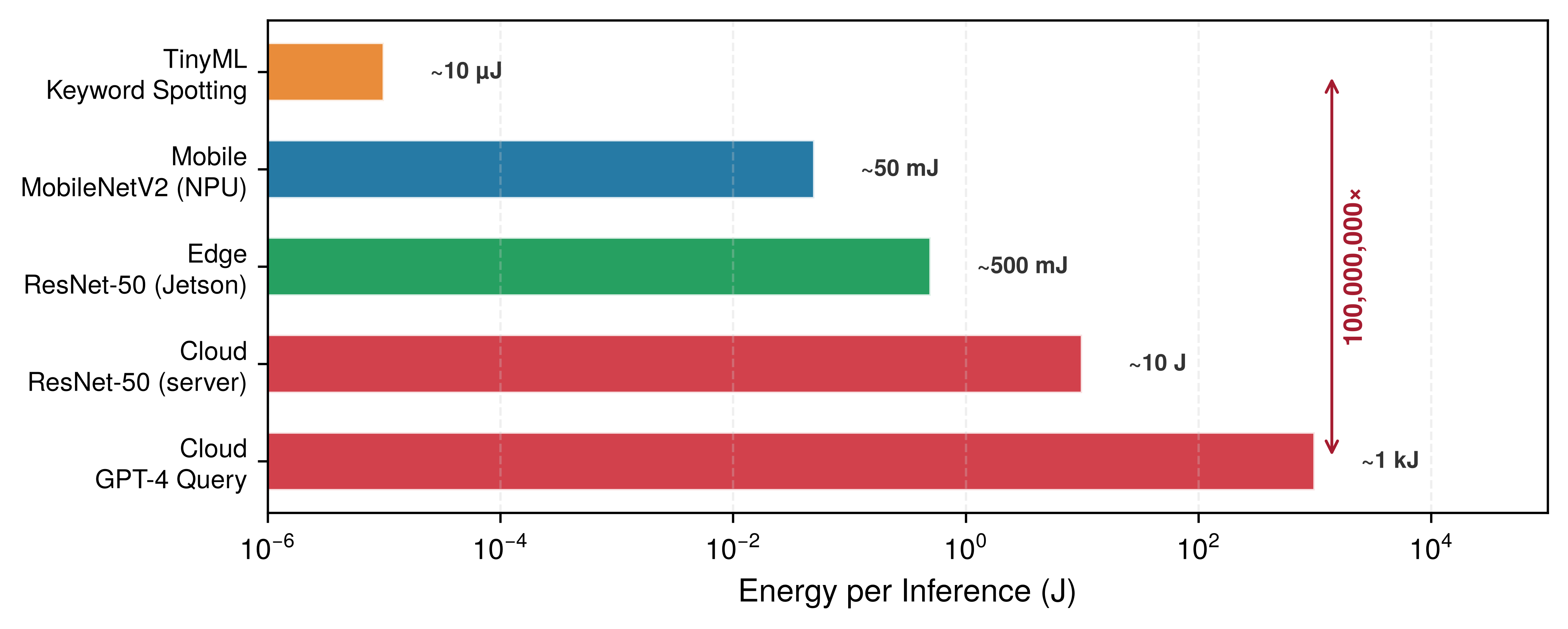
Edge ML benefits and deployment challenges
Edge ML spans wearables, industrial sensors, and smart home appliances that process data locally18 without depending on central servers. The illustrative eight-order span in figure 6 reflects different workloads and accounting boundaries, not an irreducible constant of deployment tiers.
18 Internet of things (IoT) data wall: McKinsey estimates that IoT deployments could create trillions of dollars in economic value by 2030, but those deployments depend on continuous sensor streams from devices distributed across homes, factories, farms, vehicles, and infrastructure (McKinsey Global Institute 2021). In many of those settings, the aggregate \(D_{\text{vol}}\) from raw streams overwhelms the available uplink budget or latency budget for centralized ingestion, making local edge processing an architectural requirement rather than merely a cost optimization.
McKinsey Global Institute. 2021. The Internet of Things: Catching up to an Accelerating Opportunity. McKinsey & Company.
The same energy boundary becomes a model-size boundary. Because edge devices operate within tight power envelopes, memory capacity limits what can fit while bandwidth limits how quickly the weights and activations can move. Those constraints motivate the optimization techniques covered in Model Compression, which reduce model bytes and operations to fit the hardware budget. The payoff extends beyond compute: processing raw camera feeds locally can avoid terabit-scale uplink requirements because raw data never leaves the device, reducing recurring cloud-transfer, storage, and processing costs.
The data locality invariant
The decision between local edge processing and remote cloud processing is governed by a bandwidth-latency trade-off. Remote execution is infeasible when its complete path violates the service deadline; otherwise, the faster feasible path follows from comparing complete local and remote times.
Definition 1.3: The data locality invariant
The data locality invariant first tests a complete remote path against the service deadline. Let \(T_{\text{remote}}\) denote complete remote-path time, \(T_{\text{deadline}}\) the deadline, \(\text{BW}_{\text{network}}\) offload bandwidth, \(L_{\text{lat,network}}\) network latency, and \(R_{\text{peak,remote}}\) and \(\eta_{\text{hw,remote}}\) the remote compute rate and efficiency: \[T_{\text{remote}} = \frac{D_{\text{vol}}}{\text{BW}_{\text{network}}} + L_{\text{lat,network}} + \frac{O}{R_{\text{peak,remote}} \cdot \eta_{\text{hw,remote}}}, \quad \text{remote feasible} \iff T_{\text{remote}} \le T_{\text{deadline}}\]
The corresponding \(T_{\text{local}}\) is the complete local-path time. If both paths are feasible, compare \(T_{\text{local}}\) and \(T_{\text{remote}}\); either path can be rejected by the deadline.
- Significance: The invariant defines a crossover beyond which adding remote compute \((R_{\text{peak}})\) has little effect because transmission dominates \(T_{\text{remote}}\). The local path is preferred only after its own complete execution time and resource limits are checked.
- Distinction: Unlike the iron law, which decomposes one execution path, the locality invariant compares two complete paths against each other and against an explicit service deadline.
- Common pitfall: A frequent misconception is that 5G/6G “solves” locality. While these technologies improve \(\text{BW}_{\text{network}}\), they do not remove propagation and protocol latency, so a remote path can still miss a tight service deadline.
The locality crossover is easiest to see by comparing a single high-rate sensor frame with the round-trip budget for remote processing.
Physics frames the architectural choice; the engineering trade-offs follow from it. The most immediate benefit is latency: avoiding cloud round trips can reduce response time, enabling safety-critical applications when the complete local path meets its real-time deadline. Bandwidth savings compound this advantage; for example, a retail store with 50 cameras can reduce transmission substantially by processing locally and transmitting only metadata, though the exact reduction and cost depend on codecs, traffic, and service pricing. Privacy strengthens in turn, because keeping raw data local reduces transmission exposure without eliminating other privacy obligations. For industrial deployments, operational resilience can be decisive: systems continue functioning during cloud-link outages when local power and networking remain available, a property essential where downtime carries immediate cost.
These benefits carry corresponding limitations that compound as deployments scale. In this chapter’s edge scenario, hardware provides 1–8 GB of memory and 5–50 W of power, well below the cloud-server reference.19 These constraints make model footprint, activations, runtime state, and sustainable duty cycle first-class limits. Managing distributed networks introduces complexity that scales nonlinearly with deployment size, because coordinating version control and updates across thousands of devices requires sophisticated orchestration systems,20 and hardware heterogeneity across diverse platforms demands different optimization strategies for each target.
19 Edge server constraints: In this chapter’s representative envelope, 1–8 GB can hold roughly 1–8 billion INT8 weights before activations, runtime state, and other buffers, so parameter count alone does not define a universal millions-only ceiling. Sustainable compute is further limited by power, cooling, and duty cycle.
20 Edge fleet coordination: Managing thousands of distributed edge devices introduces failure modes absent from centralized cloud: intermittent connectivity causes model version drift, hardware heterogeneity requires per-target optimization, and physical accessibility makes firmware rollbacks costly. These operational patterns are examined in ML Operations.
Napkin Math 1.7: The locality crossover
Problem: Should a drone’s object avoidance system (4K, 60 FPS) offload to the cloud, or does this become a locality crossover?
Given:
- Data \((D_{\text{vol}})\): 4K frame ≈ 24.9 MB.
- Bandwidth \((\text{BW}_{\text{network}})\): 100 Mb/s home broadband (up).
- Remote network and compute response: 110 ms (round-trip + remote compute).
Math:
- Transmission time: 24.9 MB \(\times\) 8 bits/100 Mb/s = 1,990.7 ms.
- Complete remote path: Transmission + 110 ms remote response = 2100.7 ms, vs. a 16.7 ms frame interval.
Systems insight: The remote path misses the frame interval before control-loop slack is considered, and faster remote compute cannot remove the transmission time. Cloud offload is therefore infeasible under these assumptions; the local path must still be measured to confirm that it meets the deadline.
A realistic retail deployment shows how those constraints turn into throughput, hardware, and fleet-cost requirements. Consider a smart retail chain that deploys person detection across 500 stores, each with 20 cameras/store running at 15 FPS. Table 10 cascades the per-store inference rate through YOLOv8-nano’s per-frame FLOP count to yield the throughput each store must sustain.
| Metric | Calculation | Result |
|---|---|---|
| Inferences per store | 20 cameras/store \(\times\) 15 FPS | 300 inferences/s |
| Model compute | YOLOv8-nano: 8.7 GFLOP/inference | 2610 GFLOP/s |
| Required throughput | 2610 GFLOP/s \(\times\) 2 (headroom) | ~5.22 TOPS equivalent |
Table 11 compares throughput, power, unit cost, and fleet cost for three candidate edge accelerators, including embedded GPU accelerators.
| Edge Device | INT8 TOPS | Power | Unit Cost | Fleet Cost |
|---|---|---|---|---|
| NVIDIA Jetson Orin NX | 100 TOPS | 10–25 W | $600 | $300,000 |
| Intel NUC + Movidius | 1 TOPS | 15 W | $400 | $200,000 |
| Google Coral Dev (3 boards/store) | peak 12 TOPS derated 6 TOPS |
6 W | $450 | $225,000 |
Napkin Math 1.8: Edge inference sizing
Problem: Given the throughput target in table 10 and the candidates in table 11, which edge accelerator (USB-scale TPU, workstation-class embedded GPU, or general-purpose mini-PC) delivers the required throughput at the lowest three-year fleet cost?
Math: We size from what one board sustains, not from what its datasheet peaks at. A Coral Dev Board is rated at 4 TOPS peak but delivers about 2 TOPS after 50 percent derating, so the count per store is 5.22 TOPS required ÷ 2 TOPS per board = 2.6 boards, which rounds up to 3 boards/store.
Over 3 years across 500 stores, the TCO comparison for that configuration is Hardware $225,000 + Power (0.006 kW \(\times\) 500 \(\times\) 8760 h/year \(\times\) 3 years \(\times\) $0.12/kWh = $9,460.8) = $234,460.8 total vs. a one-dedicated-cloud-GPU-per-store baseline at ~$9,855,000.
Result: One Coral alone is undersized, but the sharded configuration with 3 boards/store is the low-cost edge choice, providing 6 TOPS and about 1.3× lower per-store hardware CapEx than Jetson. Jetson remains the simpler single-device deployment when integration complexity matters more than hardware cost.
Systems insight: Edge sizing is a capacity-and-cost problem, not a device-name problem. The cheapest feasible design may be several small accelerators per site rather than one larger board, but that hardware saving must be weighed against the coordination and maintenance burden of a sharded edge fleet.
Security challenges intensify because edge devices are physically accessible: equipment deployed in retail stores or public infrastructure faces tampering risks that centralized data centers do not, requiring hardware-based protection mechanisms such as secure boot, encrypted storage, and tamper-evident enclosures. In an illustrative deployment with $500–2,000 of edge hardware per site, instrumenting 1,000 sites requires $500,000–2,000,000 upfront before installation and operations. Whether that capital cost beats cloud spending depends on utilization, labor, maintenance, and service pricing.
Real-time industrial and IoT systems
Edge applications differ by domain, but each makes the same locality argument concrete: the system cannot wait for the network, cannot ship the data, cannot expose the raw signal, or cannot stop during an outage. Autonomous vehicles represent a demanding application because safety-critical perception and control decisions must fit millisecond-scale budgets. Onboard systems process streams from multiple cameras and other sensors through local hardware; a remote cloud path cannot satisfy the tight control loop when its network delay alone exceeds the deadline.
Smart retail environments demonstrate edge ML’s practical advantages for privacy-sensitive, bandwidth-intensive applications. A checkout-free store21 can process feeds from many cameras on local edge servers, tracking customer movements and item selections without continuously transmitting raw video over a wide-area link. This architecture reduces bandwidth demand and transmission exposure, but it does not by itself ensure privacy: retention, access, secondary use, and governance controls still determine the system’s compliance and risk.
21 Checkout-free retail: A store may fuse camera observations with shelf events and transaction state locally, then transmit only selected events or aggregates. The privacy boundary must still include those derived records, because reducing raw-video transport does not determine retention, access, or secondary use.
22 Industry 4.0: The fourth industrial revolution integrates ML into the sensor-actuator feedback loop on factory floors. The systems consequence is that the control loop latency \((L_{\text{lat}})\) must be shorter than the physical process it governs: a welding robot that detects a defect at 60 Hz has a 16.7 ms sampling interval, requiring a deployment whose complete response path fits that deadline.
23 Predictive maintenance: Models analyze sensor data such as vibration and temperature to estimate equipment condition and failure risk. Continuous monitoring makes sensing cadence, duty cycle, power, and local storage first-class constraints. Battery-powered nodes may require sub-watt average operation, whereas mains-powered industrial gateways can use a much larger envelope.
The industrial IoT22 uses edge ML for applications where millisecond-level responsiveness directly impacts production efficiency and worker safety. Manufacturing facilities deploy edge ML systems for real-time quality control and predictive maintenance.23
Smart buildings use edge ML to optimize energy consumption while maintaining operational continuity during network outages. Commercial buildings equipped with edge-based building management systems process data from thousands of sensors monitoring temperature, occupancy, air quality, and energy usage. This reduces cloud transmission requirements by an order of magnitude or more while enabling sub-second response times. Healthcare applications similarly use edge ML for patient monitoring and surgical assistance, reducing data transmission while supporting low-latency workflows for real-time guidance.
Many industrial and retail edge systems are stationary and connected to site power. Recall the iron law in equation 6: local deployment removes the remote network term, while mains power makes the energy budget less restrictive than a battery’s. A factory edge server consuming hundreds of watts around the clock may be acceptable when connected to site power. Mobile devices, however, travel with their users and run on fixed battery budgets. When we shift from stationary edge infrastructure to the smartphone in a user’s pocket, a new term enters the optimization: \(\text{Energy} = \text{Power} \times T\). The dominant constraint can shift from latency to energy per inference, and with it, the engineering calculus.
Self-Check: Question
A manufacturing facility deploys 100 cameras recording uncompressed 1080p video (\(1920 \times 1080 \times 3\text{ bytes/pixel}\)) at 30 FPS. The factory has a dedicated 10 Gbps (~1.25 GB/s) fiber uplink. Why is streaming all raw video to a cloud ML server physically impossible?
- 1080p video frames contain interlaced scanlines that cloud GPUs cannot decompress.
- Fiber optic cables can only carry voice data, requiring microwave radio relays for video.
- The aggregate raw video data rate is approximately 18.7 GB/s, which exceeds the 1.25 GB/s uplink capacity by roughly 15-fold.
- Cloud object detection models require uncompressed video to be transmitted in 10-minute batched tar archives.
An autonomous drone navigates at 60 FPS (16.7 ms per-frame budget) capturing uncompressed 4K frames (~24.9 MB per frame). The drone connects via a 100 Mbps uplink to a cloud server whose round-trip latency plus inference time is 110 ms. Applying the data locality invariant, what is the feasibility of offloading this obstacle avoidance system to the cloud?
- Feasible, because the cloud GPU computes inference in under 10 ms.
- Feasible, provided 5G network slicing is enabled on the drone modem.
- Infeasible, solely because cloud servers do not support drone telemetry protocols.
- Infeasible, because transmitting a 24.9 MB frame over a 100 Mbps link requires ~2,000 ms, causing the complete remote path (~2,110 ms) to violate the 16.7 ms frame deadline by over two orders of magnitude.
Why cannot high-bandwidth wireless networking technologies (such as 5G or 6G) eliminate the need for edge ML in tight real-time control loops (\(<10\text{ ms}\))?
When sizing edge accelerators for a retail store deployment requiring 7.2 TOPS of sustained INT8 throughput, why is it inadequate to select a single accelerator rated at 8 TOPS peak datasheet throughput?
In industrial IoT manufacturing systems (Industry 4.0), the complete ML control loop latency (\(L_{\text{lat}}\)) must be strictly shorter than the ____ of the physical machinery it governs (such as a 16.7 ms window for a 60 Hz welding robot).
Mobile ML: Offline Intelligence
Edge ML solves the distance problem that limits cloud deployments by moving computation nearer to the data. Many edge systems are stationary gateways, factory servers, and retail appliances, whereas users carry phones and tablets through changing environments. Bringing the same locality to a portable device introduces a different constraint: the battery. Unlike plugged-in edge servers that can consume hundreds of watts continuously, mobile devices must operate for hours or days on fixed energy budgets.
Mobile ML addresses this challenge by integrating machine learning directly into portable devices such as smartphones and tablets, providing responsive, personalized capabilities. This paradigm excels when data locality, offline operation, and immediate response matter more than computational scale, supporting applications such as voice recognition, computational photography,24 and health monitoring. Local processing reduces transmission exposure but does not by itself guarantee privacy. These battery-powered devices must balance performance with power efficiency and thermal management, making them suited to frequent, short-duration AI tasks.
24 Computational photography: Uses ML algorithms (for example, multi-frame fusion, neural denoising) to overcome the physical limits of small mobile camera sensors. This exemplifies the mobile computing trade-off, as a multi-stage pipeline must execute within the user’s perceived shutter delay while adhering to a shared 3–5 W thermal budget.
25 Mobile vision model reduction: MobileNet-style architectures reduce the computation in common vision layers while preserving useful accuracy for mobile tasks. The architectural details appear in Network Architectures; the systems point here is that mobile deployment often requires changing the model family, not merely moving the same model to a phone.
The mobile environment introduces a critical constraint absent from stationary deployments: energy per inference becomes a first-order design parameter. Under the iron law in equation 6, cloud and edge systems optimize for minimizing \(T\), total latency. Mobile systems face an additional constraint: \(\text{Energy} = \text{Power} \times T\), and the power wall described by equation 2 caps sustained power at 3–5 W. In archetype terms, a Compute Beast workload like image classification must be transformed into a more compact vision model,25 reducing FLOPs by 13.7× while preserving enough accuracy for the application. This is not merely optimization; it represents a qualitative shift in the compute-per-byte trade-off, accepting lower peak throughput in exchange for sustainable operation within a 3–5 W thermal envelope.
This battery-and-thermal boundary gives the mobile paradigm its defining shape.
Definition 1.4: Mobile ML
Mobile machine learning is the deployment paradigm bounded by thermal design power (TDP) and battery energy.
- Significance: It is constrained by the few-watt heat dissipation capacity of passive cooling, requiring architectures that prioritize sustained energy efficiency over peak throughput \((R_{\text{peak}})\).
- Distinction: Unlike edge ML, which may have active cooling, mobile ML must operate within a personal energy budget. Unlike TinyML, it still provides a rich OS and multi-watt compute capacity.
- Common pitfall: A frequent misconception is that mobile ML performance is a fixed value. In reality, it is a time-varying constraint: performance often drops as the device hits its thermal wall, triggering throttling that reduces the duty cycle \((\eta_{\text{hw}})\).
On-device processing provides immediate responsiveness and data locality, but operates within strict electrochemical and thermodynamic boundaries. The four-branch taxonomy in figure 7 links the phone’s shared battery and passive cooling chassis to necessary NPU kernel fusions and thermal throttling limits.
The battery life and resource constraints in mobile ML translate directly into engineering requirements. Always-on ML features incur the battery tax, because continuous inference spends the phone’s finite energy budget even before the rest of the system runs.
The battery constraint limits total energy consumption over time. Even if we could ignore battery life for a plugged-in tablet or a short demo, thermodynamics imposes a second boundary. Electrical power ultimately becomes heat that the device must dissipate. A data center uses active cooling to remove this heat. A thin mobile device instead relies primarily on passive heat transfer through its chassis and surfaces. This creates the thermal wall, a hard ceiling on sustained power consumption that exists independently of battery capacity.
\begin{tikzpicture}[font=\small\sffamily]
\tikzset{
  Box/.style={inner xsep=2pt,
  draw=GreenLine,
  fill=GreenL!50,
  node distance=0.24,
    line width=0.75pt,
    anchor=west,
    text width=38mm,align=flush center,
    minimum width=32mm, minimum height=9.5mm
  },
  Box2/.style={Box,draw=BlueLine,fill=BlueL!50, text width=30mm, minimum width=30mm
  },
  Box3/.style={Box,draw=OrangeLine,fill=OrangeL!40, text width=35mm, minimum width=35mm
  },
 Box4/.style={Box,draw=VioletLine,fill=VioletL2!40, text width=32mm, minimum width=32mm
  },
 Line/.style={line width=1.0pt,black!50,text=black,-{Triangle[width=0.8*6pt,length=0.98*6pt]}},
}
\node[Box4, fill=VioletL2!90!violet!50,](B1){Binding\\ Constraint};
\node[Box2,right=2 of B1,fill=BlueL](B2){System\\ Response};
\node[Box,right=2 of B2,fill=GreenL](B3){Failure\\ Boundary};
\node[Box3,right=2 of B3,fill=OrangeL](B4){Workloads\\ That Fit};
\node[Box,draw=OliveLine,fill=OliveL!30, minimum height=11.5mm,
above=0.5of $(B2.north east)!0.5!(B3.north west)$](B0){Mobile ML};
%
\node[Box4,below=0.17 of B1](B11){Shared Battery\\ Budget};
\node[Box4,below=of B11](B12){Passive Thermal\\ Envelope};
\node[Box4,below=of B12](B13){Private Sensor\\ Data};
\node[Box4,below=of B13](B14){User Is Offline\\ or Moving};
%
\node[Box2,below=0.17 of B2](B21){Run Inference\\ on Device};
\node[Box2,below=of B21](B22){Use NPU and\\ Fused Kernels};
\node[Box2,below=of B22](B23){Compress Model\\ and Activations};
\node[Box2,below=of B23](B24){Throttle by\\ Thermal State};
%
\node[Box,below=0.17 of B3](B31){Battery\\ Tax};
\node[Box,below=of B31](B32){Thermal\\ Throttling};
\node[Box,below=of B32](B33){Storage and\\ Memory Limits};
\node[Box,below=of B33](B34){Platform Update\\ Fragmentation};
%
\node[Box3,below=0.17 of B4](B41){Computational\\ Photography};
\node[Box3,below=of B41](B42){Speech and\\ Translation};
\node[Box3,below=of B42](B43){Health\\ Monitoring};
\node[Box3,below=of B43](B44){Personalization};
%
\foreach \i in{1,2,3,4}{
\draw[Line](B1.west)--++(180:0.5)|-(B1\i);
}
\foreach \i in{1,2,3,4}{
\draw[Line](B2.west)--++(180:0.5)|-(B2\i);
}
\foreach \i in{1,2,3,4}{
\draw[Line](B3.west)--++(180:0.5)|-(B3\i);
}
\foreach \i in{1,2,3,4}{
\draw[Line](B4.west)--++(180:0.5)|-(B4\i);
}
\foreach \x in{1,2,3,4}{
\draw[Line](B0)-|(B\x);
}
\end{tikzpicture}Napkin Math 1.9: The battery tax
Problem: Consider deploying a “real-time” background object detector on a smartphone. The model consumes 2 W of continuous power when active. The phone has a standard 15 Wh battery. Can the feature stay on all day? This is the battery tax that turns battery life into a mobile ML energy-budget constraint.
Physics:
- Ideal runtime: \(\frac{15 Wh}{2 W}\) = 7.5 hours
- Reality: A user expects their phone to last 24 hours. Running this single feature continuously for a day would require 320 percent of the phone’s daily energy budget.
Systems insight: The model cannot simply be “deployed.” The techniques in Model Compression must reduce both model work and duty cycle so the feature can stay on all day.

Sustained thermal performance falls well below burst peaks.
The distinction matters for engineering decisions: the battery tax is a budget problem, solvable in principle by reducing how often the model runs or by increasing battery capacity. The thermal wall is a physics ceiling. A larger battery cannot raise the maximum sustained wattage a passive chassis can dissipate; duty-cycle and software changes can only reduce heat generation. Sustained operation above the thermal envelope triggers hardware throttling regardless of remaining battery energy. The two constraints therefore attack different points in the iron law: the battery limits total operations per charge (\(O\) integrated over time), while the thermal wall caps the instantaneous rate (\(R_{\text{peak}} \cdot \eta_{\text{hw}}\)) the silicon can sustain.
Napkin Math 1.10: The thermal wall
Problem: An unoptimized vision model requires 12 W peak compute. Can it be deployed on a mobile device, or does it hit the thermal wall and the mobile power wall?
Scenario: A mobile system-on-chip (SoC) allows approximately 3 W for passive cooling. Assume the unoptimized model ships anyway; a representative throttling trace for such a passively cooled device runs in three steps:
- Temperature rise: At 12 W, the device temperature rises at approximately 1 °C/s.
- Thermal trip: Within 60 s, the hardware reaches the thermal trip point (80 °C), triggering OS throttling.
- Throttled throughput: The 100 FPS model suddenly drops to 30 FPS to stay within the thermal envelope.
Math: Assume an illustrative 4× active-power reduction after an FP32-to-INT8 redesign (see Model Compression): 12 W ÷ 4 = 3 W, which lands right at the 3 W passive-cooling ceiling with no headroom to spare. The factor is a scenario input, not a universal whole-system guarantee from quantization alone.
Systems insight: Even a 4× power reduction does not create thermal headroom; it only just reaches the sustainable limit. Physics sets a hard ceiling that no optimization can exceed.
Mobile ML benefits and resource constraints
Mobile devices exemplify intermediate constraints: 8–16 GB RAM (varying from mid-range to flagship), 128 GB-1 TB storage, 15–45 TOPS AI compute through neural processing units26 consuming 3–5 W power. System-on-chip architectures27 integrate computation and memory to minimize energy costs. Memory capacity constrains model footprint, while 51.2–77 GB/s of bandwidth constrains how quickly weights and activations move. Battery constraints (15 Wh–22 Wh capacity) make energy optimization critical: adding 1 W of continuous ML processing to a phone that otherwise lasts 24 hours would reduce runtime to roughly 9.2 hours–11.5 hours, depending on battery capacity. Specialized on-device ML frameworks provide hardware-optimized inference for 5–50 ms UI response times.
26 Neural processing unit (NPU): A dedicated hardware block on a mobile system-on-chip whose circuits are designed for low-precision tensor operations. This specialization can improve energy efficiency relative to CPU execution, helping AI workloads fit within mobile power budgets.
27 System-on-chip (SoC): Mobile SoCs integrate CPU, GPU, and NPU cores with caches and memory controllers to reduce data-movement costs. Mobile DRAM is generally off-die, and feasible model size depends on capacity, precision, working memory, bandwidth, and latency.
28 Face ID: Apple performs facial matching within the Secure Enclave and encrypts the stored mathematical representations so that they remain available only to that subsystem and do not leave the device (Apple 2024a, 2024b). Apple reports a random false-match probability below 1 in 1,000,000 for one enrolled appearance, with higher probabilities for some populations and configurations. The example shows how local inference and hardware isolation can reduce transmission exposure while supporting low-latency authentication.
Apple. 2024a. Facial Matching Security. Apple Platform Security.
Apple. 2024b. The Secure Enclave. Apple Platform Security.
Mobile ML excels at delivering responsive experiences with stronger data locality. Real-time processing can reach sub-10 ms latency for some tasks, enabling 5–50 ms UI response times in interactive applications. Processing sensitive inputs locally reduces data transmission and central storage, and on-device enclaves such as Apple’s Secure Enclave can further protect biometric data,28 though the strength of privacy guarantees ultimately depends on the complete system design and threat model. Navigation, translation, and media-processing features can also operate without a network when their models and supporting data fit the mobile budget. Personalization rounds out the advantage, because models can exploit on-device signals and user context while keeping raw data local.
These benefits require accepting tight resource constraints. Compared to cloud deployments, mobile applications often operate under much tighter memory, storage, and latency budgets, which constrain model size and batch behavior. Battery life presents visible user impact, and thermal throttling can materially limit sustained performance: peak NPU throughput can substantially exceed what the device sustains under prolonged workloads. Development complexity multiplies across platforms, demanding separate implementations and careful performance tuning, while device heterogeneity requires multiple model variants. App-store review and staged release processes can also slow iteration compared with a service controlled entirely by its operator.
Personal assistant and media processing
Across mobile applications, the central systems problem is that several short pipelines must share the same battery and thermal budget. Computational photography exemplifies the challenge of running multiple ML pipelines within a thermal envelope. Modern flagships process each photo through multiple ML stages: portrait mode29 uses depth estimation and segmentation, night mode aligns multiple frames with ML-based denoising, and HDR merging, super-resolution, and scene optimization run in sequence. The engineering challenge is not any individual model but the pipeline: these models must share a 3–5 W power budget and complete within the user’s perceived shutter delay, requiring careful scheduling across CPU, GPU, and NPU to avoid thermal throttling.
29 Portrait Mode pipeline: This is not a single model but a sequence of real-time models for depth estimation, segmentation, and rendering. The core engineering problem is managing the pipeline’s aggregate latency and power, not any single model’s performance. The entire pipeline must execute within the user’s perceived shutter delay and share the phone’s 3–5 W thermal budget, forcing scheduling trade-offs across the CPU, GPU, and NPU to avoid throttling.
Voice-driven interactions demonstrate mobile ML’s layered architecture. Wake-word detection runs continuously on a dedicated low-power core, while speech recognition and keyboard prediction use higher-power neural processing tiers. Each layer operates at a different power tier, illustrating how mobile ML partitions workloads across heterogeneous processing units within a single SoC.
Health monitoring and augmented reality push mobile ML to its sustained-performance limits. Wearables like Apple Watch process ECG and accelerometer data on-device to reduce data transmission, while AR frameworks demand a 16.7 ms total frame budget at 60 FPS for simultaneous localization, hand tracking, and scene understanding. These applications represent the ceiling of what battery-powered, passively-cooled devices can sustain, and they define the boundary beyond which mobile optimization alone is insufficient.
These successes can create a misleading sense of ease. A common pitfall involves attempting to deploy desktop-trained models directly to mobile or edge devices without architecture modifications. Models developed on powerful workstations often fail when deployed to resource-constrained devices. A desktop ResNet-50 pipeline may require gigabytes once activations, batches, preprocessing buffers, and runtime overhead are included, even though the FP32 weights alone are about 102.4 MB. Such a pipeline, requiring 8.2 GFLOP per inference, cannot run unchanged on a representative low-end edge target with 512 MB of RAM and a 1 GFLOP/s processor. Beyond simple resource violations, desktop-optimized models may use operations unsupported by mobile hardware, assume numerical formats unavailable on embedded systems, or require batch processing incompatible with single-sample inference. Successful deployment demands architecture-aware design from the beginning: model families, arithmetic formats, and implementation choices must all match the target device.
Mobile ML demonstrates that useful intelligence can operate within a 3–5 W thermal envelope on battery power. However, smartphones still cost hundreds of dollars, require gigabytes of memory, and demand user attention to recharge daily. These requirements make them unsuitable for a vast class of applications: monitoring soil moisture across a thousand-acre farm, detecting structural stress in bridge cables, or listening for endangered species in a remote forest. These scenarios demand not just lower power but a qualitatively different engineering regime, one where the device costs dollars instead of hundreds, memory is measured in kilobytes instead of gigabytes, and the system runs unattended for months or years. Mobile optimization methods help, but they cannot bridge a 10,000-fold gap in available memory. What is needed is not a scaled-down smartphone but an entirely different class of hardware and algorithms.
Self-Check: Question
How do the battery tax and the thermal wall differ as physical constraints on mobile ML systems?
- The battery tax is an energy budget problem bounding total operations over time (\(\int \text{Power} \cdot dt\)), whereas the thermal wall is a heat dissipation ceiling bounding instantaneous sustained power (\(\text{Power} \le 2\text{--}5\text{ W}\)) regardless of battery size.
- The battery tax applies only to iOS devices, while the thermal wall applies only to Android devices.
- The battery tax can be resolved by lowering clock frequency, but the thermal wall requires increasing the clock frequency to finish calculations faster.
- The battery tax represents static memory leakage in SRAM, while the thermal wall represents network transmission power in 5G modems.
Why does deploying a mobile computational photography feature (such as Portrait Mode or Night Mode) present a pipeline scheduling challenge rather than a single-model optimization problem?
- Mobile cameras can only run one neural network per battery charge cycle.
- The feature executes a multi-stage pipeline (depth estimation, semantic segmentation, alignment, and HDR tone mapping) that must all complete within a perceived shutter delay while sharing a 2–5 W thermal budget across CPU, GPU, and NPU.
- Computational photography models cannot use quantized INT8 representations due to mathematical rounding artifacts in lens optics.
- Camera image signal processors (ISPs) operate asynchronously from the operating system and reject all external ML tensor inputs.
Why does deploying an unoptimized desktop-trained vision model (such as an FP32 ResNet-50 pipeline) directly onto a mobile device frequently fail, even when the model’s FP32 weights (~98 MB) appear smaller than the phone’s total RAM?
Running biometric matching (such as Face ID) inside a dedicated on-device Secure Enclave reduces data disclosure risks by keeping mathematical representations isolated in encrypted hardware, but it does not automatically eliminate all security or privacy risks without rigorous end-to-end system design.
Order the sequence of events that occurs when an unoptimized 12 W deep learning model runs continuously on a passively cooled 3 W smartphone SoC:
- The device temperature rises rapidly (e.g., at ~1 °C per second) as power dissipation exceeds passive cooling capacity
- The unoptimized model launches at full burst performance (e.g., 100 FPS) drawing 12 W of active compute power
- Operating system and hardware thermal controllers engage thermal throttling, reducing clock frequencies and duty cycles
- The internal SoC junction temperature reaches the critical thermal trip point (e.g., 80 °C)
- Sustained inference throughput drops precipitously (e.g., from 100 FPS to 30 FPS) to stabilize power within the 3 W TDP envelope
TinyML: Ubiquitous Sensing
Imagine instrumenting every pallet in a warehouse, every cable on a suspension bridge, every beehive in an apiary. To put “eyes and ears” on this many physical objects, tens of thousands to millions, the device must cost dollars, not hundreds of dollars, and measure millimeters, not centimeters. Smartphones are far too expensive and too large; what is needed is ubiquitous sensing at the scale of a postage stamp and the price of a cup of coffee.
TinyML completes the deployment spectrum by pushing intelligence to its physical limits: low-cost, low-power ML on deeply constrained embedded devices (Janapa Reddi et al. 2022). In this book’s operating envelope, devices costing less than $10 and consuming less than one milliwatt30 of power make ubiquitous31 sensing economically practical at massive scale; MLPerf Tiny and MCUNet show how such constraints are evaluated and optimized in practice (Banbury et al. 2021; Lin et al. 2020). This is the exclusive domain of the Tiny Constraint archetype, where the optimization objective shifts from maximizing throughput to minimizing energy per inference. Under the duty-cycle assumptions used in this chapter, a keyword spotting model consuming 10 µJ per inference can operate for years on a coin-cell battery, achieving million-fold improvements in energy efficiency by trading model capacity for operational longevity.
30 The 1 mW Threshold: Ambient energy harvesting can power a device indefinitely only when long-term harvested power exceeds the complete system’s average load. Available power varies across sources and environments—solar cells the size of a thumbnail may produce ~10 mW outdoors but ~10 µW indoors, thermoelectric generators on warm pipes ~100 µW, and RF energy from nearby transmitters ~10 µW. This crossover can transform the deployment model from “battery-limited lifetime” to “deploy and forget,” but it depends on the source, environment, and workload.
31 Ubiquitous computing: Mark Weiser’s ubiquitous-computing vision imagined computation woven into everyday environments until it receded from direct attention (Weiser 1991). TinyML is one modern path toward that vision: when the cost and power of an intelligent sensor become low enough for mass deployment, the optimization objective shifts from performance (throughput) to power (energy per inference), the central trade-off of the Tiny Constraint archetype.
Weiser, Mark. 1991. “The Computer for the 21st Century.” Scientific American 265 (3): 94–104. https://doi.org/10.1038/scientificamerican0991-94.
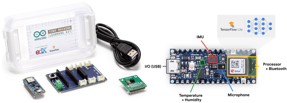
Where mobile ML requires sophisticated hardware with gigabytes of memory and multi-core processors, TinyML operates on microcontrollers32 with kilobytes of RAM and single-digit dollar price points (Banbury et al. 2021; Lin et al. 2020; Janapa Reddi et al. 2022). This radical constraint forces an entirely different approach to machine learning deployment, prioritizing ultra-low power consumption and minimal cost over computational sophistication. TinyML systems power applications such as predictive maintenance, environmental monitoring, and simple gesture recognition. The energy gap between TinyML and cloud inference (figure 6) spans at least six orders of magnitude33 and reaches eight orders for cloud LLM queries, driving entirely different system architectures and deployment models. This extraordinary efficiency enables operation for months or years on coin-cell batteries.34 In figure 8, annotated development boards illustrate this physical scale, showing integrated microcontroller chips, sensor arrays, and pin headers designed to run compact models in disconnected environments.
32 Microcontroller (MCU): A single-chip computer whose design prioritizes minimal cost and power over performance, creating the “radical constraint” mentioned. Many TinyML targets provide only tens to hundreds of kilobytes of on-chip SRAM and no virtual memory; some higher-end microcontrollers can attach external memory. The complete model, activations, and runtime state must therefore fit the memory actually available to the target, often orders of magnitude less than a smartphone provides.
Banbury, Colby, Vijay Janapa Reddi, Peter Torelli, Jeremy Holleman, Nat Jeffries, Csaba Kiraly, Pietro Montino, et al. 2021. “MLPerf Tiny Benchmark.” arXiv Preprint.
Lin, Ji, Wei-Ming Chen, Yujun Lin, John Cohn, Chuang Gan, and Song Han. 2020. “MCUNet: Tiny Deep Learning on IoT Devices.” In Advances in Neural Information Processing Systems 33: Annual Conference on Neural Information Processing Systems 2020, NeurIPS 2020, December 6-12, 2020, Virtual, edited by Hugo Larochelle, Marc’Aurelio Ranzato, Raia Hadsell, Maria-Florina Balcan, and Hsuan-Tien Lin. Curran Associates.
Janapa Reddi, Vijay, Brian Plancher, Susan Kennedy, Laurence Moroney, Pete Warden, Lara Suzuki, Anant Agarwal, et al. 2022. “Widening Access to Applied Machine Learning with TinyML.” Harvard Data Science Review 4 (1). https://doi.org/10.1162/99608f92.762d171a.
33 TinyML energy gap: This differential is rooted in hardware design philosophy; cloud GPUs are optimized for raw throughput, consuming hundreds of watts, while TinyML microcontrollers are designed for near-zero power sleep states. For ordinary cloud inference, a single request may consume about 10 joules while a specialized TinyML device uses about 10 microjoules, a \(1{,}000{,}000\times\) gap. Cloud LLM queries can push the comparison even further, as quantified in table 12.
34 Coin-cell deployment: A CR2032 battery (225 mAh at 3 V, ~675 mWh) ideally powers a complete 10–50 µW system for about 1.5–7.7 years. This “deploy-and-forget” operating model drives innovation in intermittent computing, where the device sleeps between inferences to stretch the energy budget across years of unattended operation.
Fitting the entire inference pipeline—from sensor acquisition to classification output—into these diminutive physical packages requires rethinking how model weights and runtime activations are stored in silicon.
Definition 1.5: TinyML
TinyML is the machine learning domain of always-on sensing constrained by kilobyte-scale memory and milliwatt-scale power.
- Significance: It necessitates models whose weights and code fit in flash while activations and runtime state fit in on-chip SRAM, enabling continuous inference on milliwatt power budgets.
- Distinction: Unlike mobile ML, which uses multi-watt processors and a full OS, TinyML runs on microcontrollers using bare-metal firmware or a real-time operating system.
- Common pitfall: A frequent misconception is that TinyML is just “small models.” In reality, it is an energy-bound paradigm: the primary metric is energy per inference (microjoules), not just the parameter count.
TinyML’s milliwatt-scale power consumption creates an energy gap of several orders of magnitude relative to cloud inference, with profound implications for system design. In terms of equation 6, TinyML often reaches a memory-fit constraint that the latency equation does not explicitly capture: the model footprint \(M_{\text{model}}\) and activation footprint must stay within memory capacity \(C_{\text{mem}}\). When total memory is measured in kilobytes, model structure and runtime allocation determine feasibility before latency optimization begins, and every avoidable data movement spends part of the energy budget. The objective therefore shifts from raw throughput toward energy per inference and memory fit.
Systems Perspective 1.3: Reading the energy-per-inference numbers
The energy values in table 12 combine solver-derived device-energy estimates with separate scale anchors; they are not controlled full-system measurements. An illustrative A100-only ResNet-50 bound is under 1 ms and about ~0.3 J, while an entire server can draw about ~1 kW when CPUs, memory, and overhead are included. The final-column counts show how many inferences one battery’s nominal energy could supply; they are not elapsed battery life and omit sensing, sleep, and communication.
This TinyML energy-efficiency gap helps explain why low-energy local models are attractive for always-on sensing. Actual runtime still depends on inference cadence, sleep power, sensing, communication, and the rest of the device.
The energy gap between paradigms is not a matter of degree but of scale, spanning the eight orders of magnitude sketched in figure 6. Table 12 grounds that span in concrete numbers, translating each paradigm’s energy cost into how many inferences a single smartphone battery could sustain.
| Paradigm | Example Workload | Energy/Inference | Inferences per Battery (3.7 V, 3000 mAh) |
|---|---|---|---|
| Cloud | GPT-4 query | ~1 kJ | 40 queries |
| Cloud | ResNet-50 (accelerator server) | 75.5 mJ | 529,505 queries |
| Edge | ResNet-50 (Jetson) | 15.9 mJ | 2,511,628 queries |
| Mobile | MobileNet (NPU) | 2.60 mJ | 15,393,505 queries |
| TinyML | Keyword spotting | 10 µJ | 3996 million queries |
Operating on sub-milliwatt power budgets enables continuous sensing without grid power, but forces the complete inference state into on-chip SRAM. The four-column taxonomy in figure 9 traces how kilobyte memory and duty-cycled sleep states enable always-on workloads while restricting model updates.
\begin{tikzpicture}[font=\small\sffamily]
\tikzset{
  Box/.style={inner xsep=2pt,
  draw=GreenLine,
  fill=GreenL!50,
  node distance=0.4,
    line width=0.75pt,
    anchor=west,
    text width=32mm,align=flush center,
    minimum width=32mm, minimum height=9.5mm
  },
  Box2/.style={Box,draw=BlueLine,fill=BlueL!50, text width=27mm, minimum width=27mm
  },
  Box3/.style={Box,draw=OrangeLine,fill=OrangeL!40, text width=28mm, minimum width=28mm
  },
Box4/.style={Box,draw=VioletLine,fill=VioletL2!40, text width=39mm, minimum width=39mm
  },
 Line/.style={line width=1.0pt,black!50,text=black,-{Triangle[width=0.8*6pt,length=0.98*6pt]}},
}
\node[Box4, fill=VioletL2!90!violet!50,](B1){Binding\\ Constraint};
\node[Box2,right=2 of B1,fill=BlueL](B2){System\\ Response};
\node[Box,right=2 of B2,fill=GreenL](B3){Failure\\ Boundary};
\node[Box3,right=2 of B3,fill=OrangeL](B4){Workloads\\ That Fit};
\node[Box,draw=OliveLine,fill=OliveL!30, minimum height=11.5mm,
above=0.5of $(B2.north east)!0.5!(B3.north west)$](B0){TinyML};
%
\node[Box4,below=0.37 of B1](B11){Milliwatt Power\\ Budget};
\node[Box4,below=of B11](B12){Kilobyte Memory\\ Envelope};
\node[Box4,below=of B12](B13){Always-On\\ Duty Cycle};
\node[Box4,below=of B13](B14){Sparse Network\\ Access};
%
\node[Box2,below=0.27 of B2](B21){Fit Model and\\ Activations on Chip};
\node[Box2,below=of B21](B22){Use Integer and\\ Binary Arithmetic};
\node[Box2,below=of B22](B23){Sleep Between\\ Detections};
\node[Box2,below=of B23](B24){Summarize Before\\ Transmission};
%
\node[Box,below=0.37 of B3](B31){Compression-Driven\\ Accuracy Loss};
\node[Box,below=of B31](B32){Firmware Update\\ Risk};
\node[Box,below=of B32](B33){Toolchain\\ Fragmentation};
\node[Box,below=of B33](B34){No Local\\ Full Training};
%
\node[Box3,below=0.37 of B4](B41){Wake-Word\\ Detection};
\node[Box3,below=of B41](B42){Wildlife\\ Monitoring};
\node[Box3,below=of B42](B43){Medical\\ Wearables};
\node[Box3,below=of B43](B44){Factory\\ Sensors};
%
\foreach \i in{1,2,3,4}{
\draw[Line](B1.west)--++(180:0.5)|-(B1\i);
}
\foreach \i in{1,2,3,4}{
\draw[Line](B2.west)--++(180:0.5)|-(B2\i);
}
\foreach \i in{1,2,3,4}{
\draw[Line](B3.west)--++(180:0.5)|-(B3\i);
}
\foreach \i in{1,2,3,4}{
\draw[Line](B4.west)--++(180:0.5)|-(B4\i);
}
\foreach \x in{1,2,3,4}{
\draw[Line](B0)-|(B\x);
}
\end{tikzpicture}TinyML advantages and operational trade-offs
TinyML operates at hardware extremes. Compared to cloud systems, TinyML deployments commonly provide roughly \(10^6\) to \(10^9\) times less memory, depending on whether the microcontroller budget is in low megabytes or kilobytes, with power budgets in the milliwatt range. These strict limitations enable months or years of autonomous operation35 but demand specialized algorithms, model compression, and careful systems co-design. Devices range from palm-sized developer kits to millimeter-scale chips,36 enabling ubiquitous sensing in contexts where networking, power, or maintenance are costly. Representative developer kits include the Arduino Nano 33 BLE Sense (256 KB RAM, 1 MB flash, 20–40 mW) and ESP32-CAM (520 KB RAM, 4 MB flash, 50–250 mW).
35 On-device training constraints: Full on-device training must keep intermediate layer outputs so later weight updates can reuse them, consuming memory proportional to model depth; during inference, each layer’s temporary values can usually be discarded after the next layer consumes them; during training, many of those values must remain available so the update step can decide how weights should change. With only 256 KB–2 MB RAM, full training generally exceeds this memory budget; TinyTL freezes weights and updates biases to reduce activation memory (Cai et al. 2020). This memory constraint is why TinyML devices are predominantly inference-only, with model updates pushed via firmware rather than learned in situ.
Cai, Han, Chuang Gan, Ligeng Zhu, and Song Han. 2020. “TinyTL: Reduce Activations, Not Trainable Parameters for Efficient on-Device Learning.” Advances in Neural Information Processing Systems 33: 11285–97.
36 TinyML device range: This physical range reflects a direct trade-off between deployment context and computational capability. Millimeter-scale systems prioritize minimal power (~140 µW) for single-function, long-duration tasks, whereas palm-sized boards trade larger size and higher power for the ability to process multiple complex sensor streams. This co-design choice creates a \(>10,000\times\) power and ~100\(\times\) area difference across the operational spectrum of TinyML devices.
TinyML’s extreme resource constraints paradoxically enable unique advantages. By avoiding network transmission entirely, TinyML devices avoid network-transmission latency, enabling rapid local responses for sensing and control loops without communication overhead. This self-sufficiency also transforms the economics of large-scale deployments: when per-node costs drop to single-digit dollars, instrumenting an entire factory floor, farm, or building becomes financially viable in ways that edge or cloud alternatives cannot match. Energy efficiency compounds the economic case, enabling multi-year operation on small batteries or even indefinite operation through energy harvesting. Privacy benefits follow naturally from locality, because raw data never leaves the device, reducing transmission risks and simplifying compliance. On-device processing alone does not automatically provide formal privacy guarantees without additional security mechanisms.
These capabilities require substantial trade-offs. Computational constraints impose severe limits: microcontrollers commonly provide \(10^5\) to \(10^6\) bytes of RAM, forcing models and intermediate activations into the tens-of-kilobytes to low-megabytes range depending on the workload. Development complexity requires expertise spanning neural network optimization, hardware-level memory management, embedded toolchains, and specialized debugging across diverse microcontroller architectures.
Beyond these technical constraints, operational challenges compound the difficulty. An energy-harvesting device can satisfy its long-term average power budget yet fail when stored energy is exhausted before the next harvest. Its duty cycle must therefore respect both energy per inference and the timing of available power. Model quality can suffer from aggressive compression and reduced precision, limiting suitability for applications requiring high accuracy or robustness. Deployment can also be inflexible: devices may run a small set of fixed models, and updates may require firmware workflows that are slower and riskier than cloud rollouts. Ecosystem fragmentation37 across microcontroller vendors and ML frameworks creates additional overhead and portability challenges.
37 TinyML ecosystem fragmentation: TinyML spans microcontroller families such as Arm Cortex-M, RISC-V, and Xtensa, each with different instruction sets, memory layouts, kernels, and vendor toolchains; cloud and mobile stacks also vary, but their runtimes usually hide more of this hardware diversity. A model optimized for one microcontroller target may therefore require retuning and revalidation for another, multiplying the engineering cost of multi-device deployment.
Environmental and health monitoring
TinyML applications belong here when ultra-low power, low per-node cost, and local processing make a deployment feasible that no other paradigm can sustain. Wake-word detection is the most familiar consumer example: a purpose-built low-power component listens continuously, processes audio locally, and activates higher-power components only when a wake phrase is detected, reducing average power draw.38 Precision agriculture exploits the same locality pressure from a different direction: FarmBeats used sensors, cameras, drones, and local gateway processing to reduce raw data movement where farm connectivity was costly (Vasisht et al. 2017). TinyML pushes that locality logic further when the sensing node itself must run under milliwatt budgets.
38 Always-on wake-word detection: A small, specialized model listens for the acoustic signature of a wake phrase and acts as a power gate for the higher-power application processor. The acceptable detector budget depends on the platform, but spending even a few extra milliwatts continuously can materially shorten battery life. The architecture succeeds only when the always-on path consumes far less average power than the components it prevents from waking.
Vasisht, Deepak, Zerina Kapetanovic, Jongho Won, Xinxin Jin, Ranveer Chandra, Sudipta N. Sinha, Ashish Kapoor, Madhusudhan Sudarshan, and Sean Stratman. 2017. “FarmBeats: An IoT Platform for Data-Driven Agriculture.” 14th USENIX Symposium on Networked Systems Design and Implementation (NSDI 17), 515–29.
Wildlife conservation uses TinyML for remote environmental monitoring, where solar-powered audio sensors can process continuous streams locally for species identification. Under this chapter’s illustrative payload assumptions, local analysis reduces transmission from 4.3 GB/day of raw audio to 400 KB/day of detection summaries, a 10,750× reduction. Medical wearables apply the same local-processing logic to health. Sensitivity, sampling rate, power, and battery life are device-specific validation targets rather than universal properties of TinyML hardware. Local processing can reduce continuous transmission and support privacy, while total runtime still depends on sensors, radios, duty cycle, and sleep power.
The four deployment paradigms now span the full range from megawatt data centers to milliwatt microcontrollers. Each paradigm emerged as a response to specific physical constraints, and each excels within its operating envelope. The question of how an engineer should choose among them, and what to do when no single paradigm satisfies all requirements, motivates the comparative analysis that follows.
Self-Check: Question
Comparing a dedicated TinyML keyword spotting model (~\(10\ \mu\text{J}\) per inference) to a cloud foundation model query (~\(1\text{ kJ}\) per inference), by approximately what factor does energy consumption per inference differ?
- Approximately \(100\times\) (2 orders of magnitude)
- Approximately \(10{,}000\times\) (4 orders of magnitude)
- Approximately \(100{,}000{,}000\times\) (\(10^8\), 8 orders of magnitude)
- Approximately \(10^{14}\times\) (14 orders of magnitude)
Why are microcontroller TinyML devices predominantly restricted to inference-only execution rather than full in-situ backpropagation training?
- Microcontrollers use flash memory which permanently locks all transistor gates against state changes.
- Backpropagation requires double-precision FP64 floating-point arithmetic which is mathematically impossible on 32-bit cores.
- The speed of light inside microcontroller silicon is too slow to support backward gradient propagation.
- Standard backpropagation requires storing intermediate activation tensors from every forward layer until the backward pass executes, which quickly exceeds the microcontroller’s 256 KB–2 MB on-chip SRAM capacity.
Why is the 1 mW average power threshold considered a transformative milestone in TinyML system deployment?
Why is it a fallacy to treat TinyML as merely ‘scaled-down mobile ML’ that can be addressed simply by applying standard INT8 post-training quantization?
The power management paradigm in which a battery-less or energy-harvesting microcontroller sleeps in ultra-low-power states and wakes periodically to perform inference before energy reserves deplete is called ____ computing.
Paradigm Selection
An architect choosing where to run an ML feature rarely optimizes one dimension. A privacy rule may forbid cloud processing, a latency budget may forbid remote inference, a memory footprint may exceed the mobile device, and a cost target may rule out always-on edge hardware. Cloud, edge, mobile, and TinyML are operating envelopes for those conflicts, so selecting among them requires a unified comparison framework and a structured decision process.
Comparative trade-off analysis
Deployment decisions require seeing latency-vs-throughput paradigm trade-offs side by side across the dimensions that matter. A system architect choosing between edge and mobile deployment must compare latency, power, cost, privacy, and development complexity simultaneously. Table 13 provides this comparison across fourteen dimensions, from compute power and latency to cost and deployment speed.
| Aspect | Cloud ML | Edge ML | Mobile ML | TinyML |
|---|---|---|---|---|
| Processing Location | Centralized cloud servers (Data Centers) | Local edge devices (gateways, servers) | Smartphones and tablets | Ultra-low-power microcontrollers and embedded systems |
| Latency | 100–500 ms | 10–100 ms | 5–50 ms | 1–10 ms |
| Compute Power | Very High (Multiple GPUs/TPUs) | High (Edge GPUs) | Moderate (Mobile NPUs/GPUs) | Very Low (MCU/tiny processors) |
| Storage Capacity | Cloud-scale (petabytes+) | Large (terabytes) | Moderate (gigabytes) | Very Limited (kilobytes–megabytes) |
| Energy Consumption | Very High (kW–MW range) | High (hundreds of watts) | Moderate (3–5 W) | Very Low (mW range) |
| Scalability | High (provider capacity limits) | Good (limited by edge hardware) | Moderate (per-device scaling) | Limited (fixed hardware) |
| Data Exposure | Remote processing expands the surface | Local processing reduces transmission | On-device processing reduces transmission | Raw data can remain local |
| Connectivity Required | Constant high-bandwidth | Intermittent | Optional | None |
| Offline Capability | None | Good | Excellent | Complete |
| Real-time Processing | Dependent on network | Good | Very Good | Excellent |
| Cost | High ($1000s+/month) | Moderate ($100s–$1000s) | Device purchase ($200–$1000+; often user-owned) | Very Low ($1–$10) |
| Hardware Requirements | Cloud infrastructure | Edge servers/gateways | Modern smartphones | MCUs/embedded systems |
| Development Complexity | High (cloud expertise needed) | Moderate-High (edge+networking) | Moderate (mobile SDKs) | High (embedded expertise) |
| Deployment Speed | Fast | Moderate | Fast | Slow |
This contrast reflects a common trade-off between data locality and computational scale. Remote processing increases the disclosure surface and requires additional safeguards; local processing reduces transmission and centralized-storage exposure but does not itself guarantee privacy. The archetype-paradigm mapping established in section 1.2 connects these characteristics to specific workload requirements, with each archetype gravitating toward paradigms that address its binding constraint.
No single paradigm dominates across all engineering axes. In figure 10, four-axis polar radar charts evaluate the paradigms on an ordinal 0–10 scale: subplot (a) maps raw compute and scalability against latency and energy efficiency, while subplot (b) evaluates operational autonomy across connectivity, locality, real-time response, and offline execution.
\begin{tikzpicture}[font=\sffamily]
\pgfplotsset{myaxis/.style={
   y axis line style={draw=none},
   x axis line style={draw=black,line width=1 pt},
    width=8cm,
    height=8cm,
    grid=both,
    grid style={black!30,dashed},
    tick align=inside,
    tick style={draw=none},
    ymin=0, ymax=10,
    ytick={1,3,5,7,9},
    yticklabels={},
    xtick={0,90,180,270},
    xticklabel style={align=center,font=\fontsize{8pt}{9}\selectfont\sffamily},
 % yticklabel style={font=\fontsize{7pt}{7}\selectfont\sffamily},
     yticklabel style={
     rotate around={50:(axis cs:0,0)},
     anchor=center
    },
   xlabel style={font=\fontsize{7pt}{7}\selectfont\sffamily,rotate=30},
   label distance=5pt,
   legend style={at={(1.25,1)}, anchor=north},
   legend cell align=left,
   legend style={fill=BrownL!30,draw=BrownLine,row sep=2.1pt,
   font=\fontsize{7pt}{7}\selectfont\sffamily},
      cycle list={
     {myblue,line width=1.5pt,fill=myblue!70,fill opacity=0.9},
     {mygreen,line width=1.5pt,fill=mygreen!70,fill opacity=0.4},
     {myorange,line width=1.5pt,fill=myorange!20,fill opacity=0.4},
     {myred,line width=1.5pt,fill=myred!70,fill opacity=0.4},
  },
    after end axis/.code={
      % manual y-tick labels
      \foreach \R in {1,3,5,7,9}{
      \pgfmathtruncatemacro{\newR}{\R + 0.5} %
        \node[
          font=\footnotesize\sffamily,
          anchor=base
        ]
        at (axis cs:50,\newR) {\R};
      }
    },
    legend image code/.code={
      % rectangle in Legend
      \draw[fill=#1,draw=none,fill opacity=1]
        (0pt,-2pt) rectangle (4mm,3pt);
    }
    }}
 %left graph
\begin{scope}[local bounding box=GR1,shift={(0,0)}]
\begin{polaraxis}[myaxis,
    xticklabels={Compute\\ Power, Low-Latency\\ Capability, Scalability,Energy\\ Efficiency},
]
% Cloud ML
\addplot+[]  coordinates {(0,10) (90,2) (180,10) (270,3) (360,10)};
% Edge ML
\addplot+[] coordinates {(0,8) (90,7) (180,8) (270,5) (360,8)};
% Mobile ML
\addplot+[] coordinates {(0,6) (90,8) (180,7) (270,7) (360,6)};
% TinyML
\addplot+[]  coordinates {(0,3) (90,9) (180,5) (270,10) (360,3)};
\legend{Cloud ML, Edge ML, Mobile ML, TinyML}
\addplot[draw=myblue,line width=1.5pt]   coordinates {(0,10) (90,2) (180,10) (270,3) (360,10)};
\addplot[draw=mygreen,line width=1.5pt]  coordinates {(0,8) (90,7) (180,8) (270,5) (360,8)};

\end{polaraxis}
\end{scope}
\node[below=2mm of GR1,xshift=-5mm]{\large a)};
 %right graph
\begin{scope}[local bounding box=GR2,shift={(10,0)}]
\begin{polaraxis}[myaxis,
xticklabels={Connectivity\\ Independence, Data\\ Locality, Real-time\\ Processing,Offline\\ Capability},
]
% Cloud ML
\addplot+[]  coordinates {(0,2) (90,3) (180,2) (270,2) (360,2)};
% Edge ML
\addplot+[] coordinates {(0,7) (90,7) (180,8) (270,6) (360,7)};
% Mobile ML
\addplot+[] coordinates {(0,8) (90,9) (180,7) (270,8) (360,8)};
% TinyML
\addplot+[]  coordinates {(0,10) (90,10) (180,10) (270,10) (360,10)};
%\legend{Cloud ML, Edge ML, Mobile ML, TinyML}
\addplot[draw=myblue,line width=1.5pt]  coordinates {(0,2) (90,3) (180,2) (270,2) (360,2)};
\addplot[draw=mygreen,line width=1.5pt] coordinates {(0,7) (90,7) (180,8) (270,6) (360,7)};
\end{polaraxis}
\end{scope}
\node[below=2mm of GR2]{\large b)};
\end{tikzpicture}The radar plots make the deployment decision explicit: no paradigm dominates all axes. Each paradigm concentrates complexity in a different place: cloud requires distributed-infrastructure and cost-governance expertise; edge and TinyML add fleet management, hardware diversity, and embedded constraints; mobile adds platform-specific integration and release processes. Cost structures likewise differ rather than following one ranking: cloud emphasizes recurring service expense, edge emphasizes site hardware and operations, mobile often uses user-owned devices, and TinyML trades low unit cost for specialized development and large-fleet maintenance.
A critical pitfall in deployment selection is choosing paradigms based solely on model accuracy without considering system-level constraints. A cloud-deployed model achieving 99 percent accuracy becomes useless for autonomous emergency braking if network latency exceeds reaction time requirements; a high-accuracy edge model that drains a mobile device’s battery in minutes fails despite superior accuracy. Successful deployment requires evaluating latency requirements, power budgets, network reliability, data privacy regulations, and total cost of ownership simultaneously. These constraints should be established before model development to avoid expensive architectural pivots late in the project.
Decision framework
Selecting the appropriate deployment paradigm requires a decision framework based on application constraints rather than organizational biases or technology trends. The gates are ordered by how quickly they can invalidate an architecture: privacy can make remote processing impermissible, latency can make it physically impossible, compute demand can make a local target infeasible, and cost compares the feasible survivors as operational architectures. Use figure 11 as a screening aid that organizes privacy, latency, compute-demand, and cost questions before a final architecture is selected.
\resizebox{.8\textwidth}{!}{%
\begin{tikzpicture}[line join=round,font=\small\sffamily]
\tikzset{%
Line/.style={black!50,-{Triangle[width = 5pt, length = 8pt]}, line width = 1.25pt,text=black},
LineA/.style={line width=1.0pt,black!50,latex-latex},
Box/.style={inner xsep=2pt,inner ysep=6pt,
    node distance=1.5,
    draw=BlueLine,
    line width=0.75pt,
    fill=BlueL!40,
    align=flush center,
    text width=28mm,
    minimum width=28mm, minimum height=12mm
  },
start/.style={inner xsep=2pt,draw=magenta, line width=0.75pt,  fill=magenta!07,rounded corners=8pt,
    text width=25mm,align=flush center, minimum width=25mm, minimum height=9mm},
Box3/.style={draw=VioletLine,fill=VioletL2, trapezium,aspect=1.75,inner xsep=-2ex, text width=38mm,
    node distance=1.5,font=\footnotesize\sffamily,
diamond, minimum width=35mm, minimum height=23mm,line width=0.75pt, align= flush center},
Text/.style={above,text=black!80, font=\footnotesize\sffamily},
}

\node[start](B1){Start};
\node[Box3,below=0.52 of B1](B2){Is privacy\\ critical?};
\node[Box, left=of B2](B3){Cloud Processing Allowed};
\node[Box, right=of B2](B4){Local Processing Preferred};
%
\node[Box3,below=of B2](2B1){Is low latency\\ required ($<$10 ms)?};
\node[Box, left=of 2B1](2B2){Latency\\ Tolerant};
\node[Box, right=of 2B1](2B3){Tiny or\\ Edge ML};
%
\node[Box3,below=of 2B1](3B1){Does the model require significant compute?};
\node[Box, left=of 3B1](3B2){Heavy\\ Compute};
\node[Box, right=of 3B1](3B3){Lightweight Processing};
%
\node[Box3,below=of 3B1](4B1){Are there strict\\ cost constraints?};
\node[Box,left=of 4B1](4B2){Flexible\\ Budget};
\node[Box,right=of 4B1](4B3){Low-Cost\\ Options};
%
\node[start,below =1.85 of 4B2](5B1){Edge ML};
\node[start,below =1.85 of 4B3](5B4){Tiny ML};
\node[start](5B2) at($(5B1.east)!0.28!(5B4.west)$){Cloud ML};
\node[start](5B3) at($(5B1.east)!0.73!(5B4.west)$){Mobile ML};
%arrows
\draw[Line](B1)--(B2);
\draw[Line](B2)--node[Text,pos=0.2]{No}(B3);
\draw[Line](B2)--node[Text,pos=0.2]{Yes}(B4);
\draw[Line](2B1)--node[Text,pos=0.2]{No}(2B2);
\draw[Line](2B1)--node[Text,pos=0.2]{Yes}(2B3);
\draw[Line](3B1)--node[Text,pos=0.2]{Yes}(3B2);
\draw[Line](3B1)--node[Text,pos=0.2]{No}(3B3);
\draw[Line](4B1)--node[Text,pos=0.2]{No}(4B2);
\draw[Line](4B1)--node[Text,pos=0.2]{Yes}(4B3);
%
\draw[Line](B3.south)--++(0,-13mm)-|(2B1);
\draw[Line](B4.south)--++(0,-13mm)-|(2B1);
\draw[Line](2B2.south)--++(0,-13mm)-|(3B1);
\draw[Line](2B3.south)--++(0,-13mm)-|(3B1);
\draw[Line](3B3.south)--++(0,-13mm)-|(4B1);
%
\draw[Line](4B3.south)--++(0,-6mm)-|(5B4);
\draw[Line](4B3.south)--++(0,-6mm)-|(5B3);
\draw[Line](4B2.south)--++(0,-6mm)-|(5B2);

\draw[Line](3B2.west)--++(-5mm,0)|-(5B1);

\begin{scope}[on background layer,font=\footnotesize\sffamily\bfseries]
\node[draw=GreenLine,inner xsep=8mm,inner ysep=1mm,yshift=1mm,
fill=green!02,fit=(B1)(B3)(B4)(B2),  minimum width=155mm, line width=0.35pt](BB1){};
%
\node[draw=BackLine,inner xsep=8mm,inner ysep=3mm,yshift=1mm,
fill=BackColor!10,fit=(2B1)(2B2)(2B3),  minimum width=155mm, line width=0.35pt](BB2){};
%
\node[draw=RedLine,inner xsep=8mm,inner ysep=3mm,yshift=1mm,
fill=magenta!02,fit=(3B1)(3B2)(3B3),  minimum width=155mm, line width=0.35pt](BB3){};
%
\node[draw=BrownLine,inner xsep=8mm,inner ysep=3mm,yshift=1mm,
fill=BrownL!07,fit=(4B1)(4B2)(4B3),  minimum width=155mm, line width=0.35pt](BB4){};
%
\node[draw=BlueLine,inner xsep=8mm,inner ysep=6mm,yshift=-0.85mm,
fill=cyan!03,fit=(5B1)(5B4),  minimum width=155mm, line width=0.35pt](BB5){};
%
\node[below=3pt of BB1.north east,anchor=north east]{Layer: Privacy};
\node[below=3pt of BB2.north east,anchor=north east]{Layer: Performance};
\node[below=3pt of BB3.north east,anchor=north east]{Layer: Compute Needs};
\node[below=3pt of BB4.north east,anchor=north east]{Layer: Cost};
\node[above=0pt of BB5.south east,anchor=south east]{Layer: Deployment Options};
\end{scope}
\end{tikzpicture}}The framework groups four critical decision layers rather than computing a unique answer. Privacy determines whether remote processing is permissible. Latency rejects paths that miss response-time budgets, compute demand rejects targets that cannot run the workload, and cost compares the feasible survivors. Because the drawn branches reconverge and the low-cost branch retains both mobile ML and TinyML, figure 11 narrows the design space but does not select a single paradigm.
A safety-critical braking example makes the sequencing concrete, because latency can eliminate cloud deployment before compute or cost are considered.
Example 1.1: Autonomous vehicle emergency braking
Scenario: An autonomous vehicle vision system performs real-time pedestrian detection for emergency braking under a strict 100 ms end-to-end latency budget.
Diagnosis: The scenario assumes 50–150 ms of network round-trip delay for cloud offload and 10–30 ms for local object detection on an automotive edge accelerator (300 GFLOP/s). Under those assumptions, the remote path alone causes the vehicle to travel 2.8 m before braking.
Systems lesson: Hard real-time safety constraints eliminate cloud offloading regardless of compute availability. Latency bounds dictate an Edge ML deployment architecture, reserving cloud connections for offline model training and telemetry aggregation.
This decision framework identifies technically feasible options, but feasibility does not guarantee success. Production deployment also depends on organizational capabilities that determine whether a technically sound choice can be implemented and maintained effectively.
Successful deployment requires considering factors beyond pure engineering constraints. Team expertise must align with paradigm requirements: cloud ML demands distributed systems knowledge, edge ML requires device management capabilities, mobile ML needs platform-specific optimization skills, and TinyML requires embedded systems expertise. Organizations lacking appropriate skills face extended development timelines that can undermine even the strongest technical advantages. Monitoring and maintenance capabilities similarly determine viability at scale: edge deployments require distributed device orchestration, while TinyML demands specialized firmware management that many organizations lack. Cost structures add another dimension, because the temporal pattern of expenses varies dramatically across paradigms. Cloud incurs recurring operational costs favorable for unpredictable workloads; Edge requires substantial upfront investment offset by lower ongoing costs; Mobile uses user-provided devices to minimize infrastructure expenses; and TinyML minimizes hardware costs while demanding significant development investment.
These organizational realities surface a broader concern: a machine learning approach is not always the right choice. Every ML deployment carries operational overhead (including data pipelines, monitoring, and retraining infrastructure) that simpler heuristic systems avoid, and that overhead must be justified by measurably better outcomes.
Systems Perspective 1.4: The complexity tax
Before we commit to any ML deployment, we must weigh the operational burden against simpler alternatives.
Consider a classification problem solvable by either a heuristic (if-then rules) or a deep learning pipeline. The heuristic may be fifty lines of code with near-zero compute cost, about one hour per month to update rules, and no model drift. The ML system may still have only fifty lines of model code, but it also brings roughly 2,000 lines of infrastructure for data pipelines, monitoring, and GPU drivers, plus about 40 hours per month debugging drift and managing infrastructure.
An ML system that improves accuracy from 90 percent to 95 percent may still be a poor engineering choice if it introduces a 40\(\times\) increase in complexity. ML systems engineering is the art of minimizing this tax through robust architecture. If the operational cost of maintaining model quality over time is unaffordable, the simpler heuristic may be the superior systems choice.
That comparison turns model choice into a system-design decision spanning physics, infrastructure cost, and the ongoing burden of maintaining accuracy. When the complexity tax exceeds the accuracy gain, the simpler heuristic is the superior systems choice.
Checkpoint 1.2: System design
The central trade-off is often accuracy vs. complexity.
Decision gates
Successful deployment balances technical optimization against organizational capability. Paradigm selection extends well beyond technical requirements to encompass team skills, operational capacity, and economic constraints, all bounded by the physical scaling laws developed in this chapter. ML Operations and Benchmarking develop the operational and measurement consequences. In practice, however, the decision framework rarely points to a single winner. Most production systems combine multiple paradigms, such as training in the cloud, serving at the edge, and preprocessing on mobile, to satisfy constraints that no single deployment target can meet alone.
Self-Check: Question
In the four-layer deployment screening decision framework, why is the Privacy layer evaluated first, followed by Latency, Compute Demand, and Cost?
- The layers are ordered by how rapidly a hard constraint can completely invalidate an architecture: legal/privacy rules may forbid remote transmission entirely, physical latency limits can make cloud offload impossible, compute demands eliminate undersized devices, and cost compares the remaining feasible survivors.
- Privacy is the easiest parameter to optimize in software using compiler flags, whereas cost cannot be calculated until after deployment.
- Cloud providers require privacy agreements before allowing access to GPU instances.
- The framework is ordered purely alphabetically based on traditional software engineering conventions.
An autonomous vehicle travels at 100 km/h (~27.8 m/s). An emergency pedestrian detection system evaluates two architectures: (1) an automotive Edge ML accelerator with a 15 ms local detection latency, and (2) a Cloud ML server with 115 ms total latency (100 ms network RTT + 15 ms compute). How much additional distance does the vehicle travel before braking begins if the cloud architecture is used?
- 0.28 meters
- Approximately 2.8 meters
- Approximately 28 meters
- Exactly 100 meters
What is the complexity tax in ML systems engineering, and when is a simple heuristic (e.g., rule-based logic or regular expressions) superior to a deep learning pipeline?
In ML systems engineering, selecting a deployment paradigm based solely on benchmark model accuracy is a sound practice because hardware infrastructure can always be scaled to meet application constraints later.
What is the Total Cost of Ownership (TCO) calculation, and why must ML architects evaluate TCO rather than hardware purchase price or cloud VM hourly rates alone when selecting a deployment paradigm?
Hybrid Architectures
The decision framework (figure 11) narrows the feasible paradigms for a given application. In practice, production systems rarely use just one paradigm. Voice assistants combine TinyML wake-word detection with mobile speech recognition and cloud natural language understanding. Autonomous vehicles pair edge inference for real-time perception with cloud training for model updates. These hybrid architectures exploit the strengths of multiple paradigms while mitigating their individual weaknesses. Three integration strategies formalize how such combinations work in practice.
Integration patterns
The three essential hybrid ML patterns differ by which boundary creates the constraint: train-serve split, hierarchical processing, or progressive deployment. Their selection is an iron-law decision: each stage should run where its binding term, whether training compute, local latency, or model size, is cheapest to satisfy.
The train-serve split places training in the cloud while inference happens on edge, mobile, or tiny devices. This pattern exploits cloud scale for training while benefiting from local inference latency and data locality. When a trained artifact serves many requests, its fixed training cost can be amortized across repeated inference.39
39 Train-serve cost asymmetry: Training usually requires many forward and backward passes, whereas one inference request uses a trained artifact for one or more forward passes. Training is not literally one-time because models may be retrained, and inference cost varies sharply with model size, sequence length, batching, and service overhead. The economic rationale for the split is amortization: repeated use can spread each training cycle’s fixed cost across many served predictions.
Definition 1.6: Hybrid ML
Hybrid machine learning is the deployment strategy that distributes an ML pipeline across two or more deployment tiers, assigning each stage according to its latency, compute, data, and operational constraints.
- Significance: Hybrid architectures exploit the iron law’s additive structure: the edge tier can reduce \(L_{\text{lat}}\) for time-sensitive preprocessing and inference, while the cloud tier can provide the \(R_{\text{peak}}\) needed for training, retraining, and heavy batch inference. The split follows the data locality invariant: compare each stage’s complete local and remote paths, reject paths that miss the service deadline, and then choose among the feasible alternatives.
- Distinction: Unlike cloud-only deployment (which accepts the distance penalty for all stages) or edge-only deployment (which accepts limited \(R_{\text{peak}}\) for all stages), hybrid ML dynamically assigns each pipeline stage to the tier where its binding iron law term is minimized.
- Common pitfall: A frequent misconception is that hybrid ML is just “running two models.” In reality, the participating tiers must share synchronized state—feature definitions, model versions, and preprocessing logic—so that their paths produce consistent results. Without this synchronization, training-serving skew emerges at tier boundaries.
In hierarchical processing, data and intelligence flow between computational tiers. TinyML sensors perform basic anomaly detection, edge devices aggregate and analyze data from multiple sensors, and cloud systems handle complex analytics and model updates. Each tier handles tasks appropriate to its capabilities.
The third pattern, progressive deployment, systematically compresses models for deployment across tiers. A large cloud model becomes progressively optimized versions for edge servers, mobile devices, and tiny sensors. Voice assistants exemplify this pattern: wake-word detection uses small, always-on models, often tens of kilobytes for benchmark TinyML neural networks and sub-milliwatt to milliwatt-scale power on dedicated low-power hardware, while complex natural language understanding requires much larger models in cloud infrastructure.
With three integration patterns available, selection becomes a constraint-matching problem: choose the pattern whose trade-off profile matches the system’s dominant bottleneck. Table 14 summarizes the trade-off, the conditions that favor each pattern, and the conditions that argue against it.
| Pattern | Trade-off | Choose when | Avoid when |
|---|---|---|---|
| Train-Serve Split | Training cost vs. inference latency | Training requires scale that inference does not; privacy matters for inference but not training | Model needs continuous learning from deployed data |
| Hierarchical Processing | Local autonomy vs. global optimization | Data volume exceeds transmission capacity; decisions needed at multiple timescales | All processing can occur at one tier; network is reliable and fast |
| Progressive Deployment | Model quality vs. deployment reach | Same model needed at multiple capability levels; graceful degradation required | Model cannot be meaningfully compressed; single deployment target |
Voice assistants combine train-serve split, progressive deployment, and hierarchical processing; autonomous vehicles combine hierarchical processing with progressive deployment to run optimized models at each tier. Privacy-preserving distributed training approaches extend this menu when data should remain close to the devices that produce it.
Production system integration
Production hybrid systems coordinate multiple tiers through structured interaction channels. In figure 12, labeled connection vectors illustrate this multi-tier architecture, showing how trained model artifacts deploy downward while sensor streams and intermediate inference results propagate upward to centralized analytics.
\begin{tikzpicture}[font=\small\sffamily]
\tikzset{
Line/.style={line width=1.0pt,black!50,text=black},
  Box/.style={inner xsep=2pt,
    node distance=0.6,
    draw=GreenLine, line width=0.75pt,
    fill=GreenL,
    text width=20mm,align=flush center,
    minimum width=20mm, minimum height=9mm
  },
   Text/.style={inner xsep=2pt,
    draw=none, line width=0.75pt,
    fill=TextColor,
    font=\footnotesize\sffamily,
    align=flush center,
    minimum width=7mm, minimum height=5mm
  },
  }

\node[Box,fill=RedL,draw=RedLine](G2){Training};
\node[Box,fill=none,draw=none,below =1.2 of G2](A){};
\node[Box,node distance=2.25, left=of A](B2){Inference};
\node[Box,node distance=2.25,left=of B2,fill=BlueFill,draw=BlueLine](B1){Inference};
\node[Box,node distance=2.25, right=of A,fill=OrangeFill,draw=OrangeLine](B3){Inference};
%
\node[Box,node distance=1.15, below=of B1,fill=BlueFill,draw=BlueLine](1DB1){Processing};
\node[Box,node distance=1.15, below=of B3,fill=OrangeFill,draw=OrangeLine](1DB3){Processing};
\path[](1DB3)-|coordinate(S)(G2);
\node[Box,node distance=1.5,fill=RedL,draw=RedLine]at(S)(1DB2){Analytics};
\path[](G2)-|coordinate(SS)(B2);
\node[Box](G1)at(SS){Sensors};
%
\scoped[on background layer]
\node[draw=BackLine,inner xsep=4mm,inner ysep=6mm,anchor= west,
       yshift=1mm,fill=BackColor,fit=(G1)(B2),line width=0.75pt](BB2){};
\node[below=3pt of  BB2.north,anchor=north]{TinyML};
%
\scoped[on background layer]
\node[draw=BackLine,inner xsep=4mm,inner ysep=7mm,anchor= west,
       yshift=0mm,fill=BackColor,fit=(G2)(1DB2),line width=0.75pt](BB2){};
\node[below=3pt of  BB2.north,anchor=north]{Cloud ML};
%
\draw[Line,-latex](G1.west)--++(180:0.9)|-node[Text,pos=0.1]{Data}(B2);
\draw[Line,-latex](G2)--++(270:1.20)-|(B2);
\draw[Line,-latex](G2)--++(270:1.20)-|(B3);
\draw[Line,-latex](G2)--node[Text,pos=0.46]{Deploy}++(270:1.20)-|(B1);
%
\draw[Line,-latex](B1)--node[Text,pos=0.5]{Results}(1DB1);
\draw[Line,-latex](B2)|-node[Text,pos=0.75]{Results}(1DB1.10);
%
\draw[Line,-latex](B1.330)--++(270:0.9)-|node[Text,pos=0.2]{Assist}(B3.220);
\draw[Line,-latex](B2.east)--node[Text,pos=0.5]{Sync}++(0:5.4)|-(1DB3.170);
%
\draw[Line,-latex](1DB1.350)--node[Text,pos=0.75]{Results}(1DB2.190);
\draw[Line,-latex](1DB3.190)--node[Text,pos=0.50]{Data}(1DB2.350);
\draw[Line,-latex](B3.290)--node[Text,pos=0.5]{Results}(1DB3.70);
%
\scoped[on background layer]
\node[draw=BackLine,inner xsep=4mm,inner ysep=5mm,anchor= west,
      yshift=-2mm,fill=BackColor,fit=(B1)(1DB1),line width=0.75pt](BB2){};
\node[above=3pt of  BB2.south,anchor=south]{Edge ML};
%
\scoped[on background layer]
\node[draw=BackLine,inner xsep=4mm,inner ysep=5mm,anchor= west,
      yshift=-2mm,fill=BackColor,fit=(B3)(1DB3),line width=0.75pt](BB2){};
\node[above=3pt of  BB2.south,anchor=south]{Mobile ML};
\end{tikzpicture}Production systems demonstrate these integration patterns by placing each tier boundary at a different binding constraint. Industrial defect detection exemplifies Train-Serve Split: cloud infrastructure trains vision models on datasets from multiple facilities, then distributes optimized versions to edge servers managing factory floors, tablets for quality inspectors, and embedded cameras on production lines. Agricultural monitoring illustrates Hierarchical Processing: soil sensors perform local anomaly detection at the TinyML tier, edge processors aggregate data from dozens of sensors and identify field-level patterns, while cloud infrastructure handles farm-wide analytics and seasonal planning. Fitness tracking exemplifies Progressive Deployment with gateway patterns: wearables continuously monitor activity using microcontroller-optimized algorithms consuming \(<1\text{ mW}\), sync processed summaries to smartphones that combine metrics from multiple sources, then transmit periodic updates to cloud infrastructure for longitudinal health analysis.
Why hybrid approaches work
The four deployment paradigms differ in physical resource budgets but share systems engineering foundations. In figure 13, a three-tier vertical hierarchy traces how top-level deployment targets depend on shared data, compute, and architectural principles, which in turn support cross-cutting efficiency and reliability considerations.
This convergence explains why techniques transfer between scales when they attack a shared bottleneck. Cloud-trained models can deploy to edge because the learned weights and operator graph can be reused, but the target device changes the memory, precision, latency, and power budget. Lower-precision representations developed for edge deployment reduce cloud serving costs; Model Compression formalizes these methods as quantization. Strategies for splitting work across devices likewise inform edge deployments that partition one model across more than one processor; Model Training formalizes this family as model parallelism.
Mobile optimization insights inform cloud efficiency because memory bandwidth constraints appear at every scale. Methods that reduce memory traffic on phones can also reduce cloud inference costs when applied to batch serving. TinyML’s extreme constraints likewise motivate compact representations and memory-management techniques that can inform larger systems under similar memory pressure.
\begin{tikzpicture}[font=\small\sffamily]
  \tikzset{
    Box/.style={draw=none,minimum width=38mm, minimum height=20mm, node distance=7mm},
    Arr/.style={-{Triangle[width=10pt,length=8pt]}, line width=5pt,cyan!40,shorten >=1pt, shorten <=2pt},
 Box2/.style={align=flush center, inner xsep=2pt,draw=none,
  font=\footnotesize\sffamily\bfseries, line width=0.75pt, fill=OrangeL!30, text width=38mm,
    minimum width=36mm, minimum height=7mm},
  Box3/.style = {Box2,draw=none,fill=cyan!10},
  Box4/.style = {Box2,draw=none,fill=GreenFill!60},
LineA/.style = {violet!60,{Circle[line width=1.0pt,fill=white,length=5.5pt]}-,line width=1.5pt,shorten <=-3pt},
    Arr/.style={-{Triangle[width=14pt,length=11pt]}, line width=8pt,black!40,shorten >=1pt, shorten <=2pt},
Txt/.style = {font=\footnotesize\sffamily,black!80,align=center}
}
\tikzset{
pics/stitAI/.style = {
        code = {
        \pgfkeys{/channel/.cd, #1}
\def\inset{2.2pt} %
\def\myshape{%
  (0,1.34) to[out=220,in=0] (-1.20,1.03) --
  (-1.20,-0.23) to[out=280,in=160] (0,-1.53) to[out=20,in=260] (1.20,-0.23) --
  (1.20,1.03)  to[out=180,in=320] cycle
}
\begin{scope}[shift={($(0,0)+(0,0)$)},scale=\scalefac,every node/.append style={transform shape}]
 \begin{scope}
 \clip[] \myshape;
 \draw[fill=\filllcolor,draw=\drawcolor!60, line width=3*\inset] \myshape;
\end{scope}
\node[draw=\drawcolor,line width=\Linewidth,rounded corners=4pt, fill=\filllcirclecolor,
font=\huge\sffamily,minimum size=13mm](AI) at(-1.1,-0.1){AI};
\draw[blue,rounded corners,line width=\Linewidth,-{Circle[blue,fill=yellow,length=6.5pt]}]
(AI.30)--++(3mm,0)--++(0,3mm)--++(6mm,0);
\draw[green!60!black,rounded corners,line width=\Linewidth,-{Circle[green!60!black,fill=yellow,length=6.5pt]}]
(AI.0)--++(9mm,0);
\draw[red,rounded corners,line width=\Linewidth,-{Circle[red,fill=yellow,length=6.5pt]}]
(AI.330)--++(3mm,0)--++(0,-3mm)--++(6mm,0);
\end{scope}
    }
  }
}
%cloud ML
\tikzset {
pics/cloudA/.style = {
        code = {
        \pgfkeys{/channel/.cd, #1}
\begin{scope}[local bounding box=CLO,scale=\scalefac, every node/.append style={transform shape}]
\node[draw=\drawcolor!90!red,line width=\Linewidth,minimum width=6mm,minimum height=12mm](VSK)at(0,0.5){};
\node[draw=\drawcolor!90!red,line width=\Linewidth,fill=white,minimum width=9mm,minimum height=4mm](VSKG)at(VSK.north){};
\node[draw=\drawcolor!90!red,line width=\Linewidth,fill=white,minimum width=9mm,minimum height=4mm](VSKC)at(VSK.center){};
\node[draw=\drawcolor!90!red,line width=\Linewidth,fill=white,minimum width=9mm,minimum height=4mm](VSKD)at(VSK.south){};
\draw[fill=\filllcolor,draw=\drawcolor!60,,line width=\Linewidth](0,0)to[out=170,in=180,distance=11](0.1,0.61)
to[out=90,in=105,distance=17](1.07,0.71)
to[out=20,in=75,distance=7](1.48,0.36)
to[out=350,in=0,distance=7](1.48,0)--(0,0);
\draw[draw=\drawcolor!60,,line width=\Linewidth](0.27,0.71)to[bend left=25](0.49,0.96);
\draw[draw=\drawcolor!60,,line width=\Linewidth](0.67,1.21)to[out=55,in=90,distance=13](1.5,0.96)
to[out=360,in=30,distance=9](1.68,0.42);
\node[single arrow, draw=orange,fill=orange,
      minimum width = 10pt, single arrow head extend=3pt,
      minimum height=10mm,
      rotate=270]at(1.05,0) {};
\end{scope}
}
}
}
    % #1 number of teeths
    % #2 radius intern
    % #3 radius extern
    % #4 angle from start to end of the first arc
    % #5 angle to decale the second arc from the first
    % #6 inner radius to cut off
    \tikzset{
      pics/gear/.style args={#1/#2/#3/#4/#5/#6/#7}{
       code={
               \pgfkeys{/channel/.cd, #7}
    \begin{scope}[shift={($(0,0)+(0,0)$)},scale=\scalefac,every node/.append style={transform shape}]
        \pgfmathtruncatemacro{\N}{#1}%
        \def\rin{#2}\def\rout{#3}\def\aA{#4}\def\aOff{#5}\def\rcut{#6}%
        \path[rounded corners=1.5pt,draw=\drawcolor,fill=\filllcolor]
          (0:\rin)
          \foreach \i [evaluate=\i as \n using (\i-1)*360/\N] in {1,...,\N}{%
            arc (\n:\n+\aA:\rin)
            -- (\n+\aA+\aOff:\rout)
            arc (\n+\aA+\aOff:\n+360/\N-\aOff:\rout)
            -- (\n+360/\N:\rin)
          } -- cycle;
          \draw[draw=none,fill=white](0,0) circle[radius=\rcut];
    \end{scope}
      }}
    }

\tikzset {
pics/cloudML/.style = {
        code = {
        \pgfkeys{/channel/.cd, #1}
\begin{scope}[local bounding box=CLO,scale=\scalefac, every node/.append style={transform shape}]
\draw[fill=\filllcolor,draw=\drawcolor!60,,line width=\Linewidth](0,0)to[out=170,in=180,distance=11](0.1,0.61)
to[out=90,in=105,distance=17](1.07,0.71)
to[out=20,in=75,distance=7](1.48,0.36)
to[out=350,in=0,distance=7](1.48,0)--(0,0);
\draw[draw=\drawcolor!60,,line width=\Linewidth](0.27,0.71)to[bend left=25](0.49,0.96);
%\draw[draw=\drawcolor!60,,line width=\Linewidth](0.67,1.21)to[out=55,in=90,distance=13](1.5,0.96)
%to[out=360,in=30,distance=9](1.68,0.42);
%\node[single arrow, draw=orange,fill=orange,
   %   minimum width = 10pt, single arrow head extend=3pt,
   %   minimum height=10mm,
   %   rotate=270]at(1.05,0) {};
 \draw[red,rounded corners,line width=\Linewidth,-{Circle[red,fill=yellow,length=6.5pt]}]
(0.3,0.1)--++(0,-8mm)--++(-5mm,0);
 \draw[violet,rounded corners,line width=\Linewidth,-{Circle[violet,fill=yellow,length=6.5pt]}]
(0.7,0.1)--++(0,-10mm);
 \draw[blue,rounded corners,line width=\Linewidth,-{Circle[blue,fill=yellow,length=6.5pt]}]
(1.1,0.1)--++(0,-8mm)--++(5mm,0);
\pic[shift={(0,0)}] at (0.65,0.1) {gear={12/1.5/1.9/8/4/0.8/scalefac=0.35,
drawcolor=mypurple,filllcolor=mypurple}};
\end{scope}
}
}
}
\tikzset {
pics/mobile/.style = {
        code = {
        \pgfkeys{/channel/.cd, #1}
\begin{scope}[local bounding box=MOB,scale=\scalefac, every node/.append style={transform shape}]
\node[rectangle,draw=\drawcolor,minimum height=94,minimum width=47,
            rounded corners=4,thick,fill=white](R1){};
\node[rectangle,draw=\drawcolor,minimum height=67,minimum width=38,thick,fill=\filllcolor](R2){\Large AI};
\node[circle,minimum size=8,below= 2pt of R2,inner sep=0pt,thick,fill=\filllcirclecolor]{};
\node[rectangle,fill=\filllcirclecolor,minimum height=1,minimum width=20,above= 4pt of R2,inner sep=0pt,thick]{};
%
 \end{scope}
     }
  }
}
%brain
\tikzset{pics/brain/.style = {
        code = {
        \pgfkeys{/channel/.cd, #1}
\begin{scope}[local bounding box=BRAIN,scale=\scalefac, every node/.append style={transform shape}]
\draw[fill=\filllcolor,line width=\Linewidth](-0.3,-0.10)to(0.08,0.60)
to[out=60,in=50,distance=3](-0.1,0.69)to[out=160,in=80](-0.26,0.59)to[out=170,in=90](-0.46,0.42)
to[out=170,in=110](-0.54,0.25)to[out=210,in=150](-0.54,0.04)
to[out=240,in=130](-0.52,-0.1)to[out=300,in=240]cycle;
\draw[fill=\filllcolor,line width=\Linewidth]
(-0.04,0.64)to[out=120,in=0](-0.1,0.69)(-0.19,0.52)to[out=120,in=330](-0.26,0.59)
(-0.4,0.33)to[out=150,in=280](-0.46,0.42)
%
(-0.44,-0.03)to[bend left=30](-0.34,-0.04)
(-0.33,0.08)to[bend left=40](-0.37,0.2) (-0.37,0.12)to[bend left=40](-0.45,0.14)
(-0.26,0.2)to[bend left=30](-0.24,0.13)
(-0.16,0.32)to[bend right=30](-0.27,0.3)to[bend right=30](-0.29,0.38)
(-0.13,0.49)to[bend left=30](-0.04,0.51);
\draw[rounded corners=0.8pt,line width=\Linewidth,\drawcircle,-{Circle[fill=\filllcolor,length=2.5pt]}](-0.23,0.03)--(-0.15,-0.03)--(-0.19,-0.18)--(-0.04,-0.28);
\draw[rounded corners=0.8pt,line width=\Linewidth,\drawcircle,-{Circle[fill=\filllcolor,length=2.5pt]}](-0.17,0.13)--(-0.04,0.05)--(-0.06,-0.06)--(0.14,-0.11);
\draw[rounded corners=0.8pt,line width=\Linewidth,\drawcircle,-{Circle[fill=\filllcolor,length=2.5pt]}](-0.12,0.23)--(0.31,0.0);
\draw[rounded corners=0.8pt,line width=\Linewidth,\drawcircle,-{Circle[fill=\filllcolor,length=2.5pt]}](-0.07,0.32)--(0.06,0.26)--(0.16,0.33)--(0.34,0.2);
\draw[rounded corners=0.8pt,line width=\Linewidth,\drawcircle,-{Circle[fill=\filllcolor,length=2.5pt]}](-0.01,0.43)--(0.06,0.39)--(0.18,0.51)--(0.31,0.4);
\end{scope}
     }
  }
}
\tikzset{mycylinder/.style={cylinder, shape border rotate=90, aspect=1.3, draw, fill=white,
minimum width=25mm,minimum height=11mm,line width=\Linewidth,node distance=-0.15},
pics/dataP/.style = {
        code = {
        \pgfkeys{/channel/.cd, #1}
\begin{scope}[local bounding box=STREAMING,scale=\scalefac, every node/.append style={transform shape}]
\node[mycylinder,fill=\filllcolor!50] (A) {};
\node[mycylinder, above=of A,fill=\filllcolor!50] (B) {};
\node[mycylinder, above=of B,fill=\filllcolor!10] (C) {};
\fill[\filllcolor!50!black]($(C.west)!0.12!(C.east)$)circle(3pt);
\fill[\filllcolor!50!black]($(B.west)!0.12!(B.east)$)circle(3pt);
\fill[\filllcolor!50!black]($(A.west)!0.12!(A.east)$)circle(3pt);
%
\draw[draw=\drawcolor,line width=2.5*\Linewidth](B.east)--++(17mm,0);
\node[draw=\drawcolor,line width=\Linewidth,minimum width=9mm,fill=white,minimum height=22mm](BD)at($(B.east)+(8mm,0)$){};
\node[draw=\drawcolor,line width=\Linewidth,minimum width=5mm,minimum height=8mm,fill=white](BDM)at($(BD.east)+(5mm,0)$){};
\node[circle,draw=orange,line width=\Linewidth,minimum size=5mm]at($(BD.north)!0.2!(BD.south)$){};
\node[rectangle,draw=blue,line width=\Linewidth,minimum size=5mm]at($(BD.north)!0.5!(BD.south)$){};
\node[circle,draw=green,line width=\Linewidth,minimum size=5mm]at($(BD.north)!0.8!(BD.south)$){};
\end{scope}
     }
  }
}
\tikzset {
pics/hand/.style = {
        code = {
        \pgfkeys{/channel/.cd, #1}
\begin{scope}[local bounding box=MOB,scale=\scalefac, every node/.append style={transform shape}]
\draw[draw=\drawcolor,line width=\Linewidth,fill=\filllcirclecolor](1.07,-0.02)--(1.70,0.2)arc(110:-40:1.0mm)--(1.0,-0.48)arc(-60:-100:4.0mm)--(0.4,-0.34)--(0.15,-0.42)
--(-0.1,0.13)--(0.31,0.33)--(1,0.08)to [bend left=25]cycle;
\draw[draw=\drawcolor,line width=\Linewidth](-0.1,0.13)--(0.31,0.33)--(1,0.08)arc(60:-90:1.4mm)--(0.55,-0.03);
\node[draw=\drawcolor,line width=\Linewidth,fill=cyan ,minimum width=8mm,minimum height=5mm,rotate=117]at(-0.17,-0.26){};
 \end{scope}
     }
  }
}
\tikzset{%
 LineST/.style={-{Circle[\drawcolor,fill=white,length=7pt]},draw=\drawcolor,line width=\Linewidth,rounded corners},
 ellipseST/.style={fill=\filllcolor,ellipse,minimum width = 2.5mm, inner sep=2pt, minimum height =1.5mm},
 BoxST/.style={line width=\Linewidth,fill=white,draw=\drawcolor,rectangle,minimum width=56,minimum height=16
 ,rounded corners=2pt},
 pics/streaming/.style = {
        code = {
        \pgfkeys{/channel/.cd, #1}
\begin{scope}[local bounding box=STREAMING,scale=\scalefac, every node/.append style={transform shape}]
\node[BoxST,minimum width=44,minimum height=48](\picname-RE1){};
\foreach \i/\j in{1/north,2/center,3/south}{
\node[BoxST](\picname-GR\i)at(\picname-RE1.\j){};
\node[ellipseST]at($(\picname-GR\i.west)!0.2!(\picname-GR\i.east)$){};
\node[ellipseST]at($(\picname-GR\i.west)!0.4!(\picname-GR\i.east)$){};
}
\draw[LineST](\picname-GR1.40)--++(0,0.5)--++(1,0)coordinate(\picname-C1);
\draw[LineST](\picname-GR1)--++(2,0)coordinate(\picname-C2);
\draw[LineST](\picname-GR2)--++(1.8,0)coordinate(\picname-C3);
\draw[LineST](\picname-GR3)--++(2,0)coordinate(\picname-C4);
\draw[LineST](\picname-GR3.320)--++(0,-0.5)--++(1,0)coordinate(\picname-C5);
\draw[LineST](\picname-GR3.220)--++(0,-0.5)--++(-1,0)coordinate(\picname-C6);
\draw[LineST](\picname-GR3)--++(-2,0)coordinate(\picname-C7);
\draw[LineST](\picname-GR2)--++(-1.8,0)coordinate(\picname-C8);
\draw[LineST](\picname-GR1)--++(-2,0)coordinate(\picname-C9);
\draw[LineST](\picname-GR1.140)--++(0,0.5)--++(-1,0)coordinate(\picname-C10);
 \end{scope}
     }
  }
}
\tikzset{pics/light/.style = {
        code = {
        \pgfkeys{/channel/.cd, #1}
\begin{scope}[local bounding box=LIGHT,scale=\scalefac, every node/.append style={transform shape}]
 \draw[draw=\drawcolor,fill=\filllcolor,line width=\Linewidth](0,0)to[out=135,in=310](-0.18,0.5) to[out=125,in=230](-0.25,1.55)
  to[out=50,in=130,distance=14](0.89,1.55)  to[out=310,in=55](0.84,0.55)to[out=230,in=50](0.64,0) --cycle;
 \foreach \i in {0.13,0.23,0.33,0.43}{
\node[fill=\filllcolor!30!black,rounded corners=0.5pt,rectangle,minimum width=19,minimum height=2,inner sep=0pt,rotate=4]at(0.30,-\i){};
}
 \draw[draw=none,fill=\filllcolor!30!black,rounded corners=1pt](-0.03,-0.54)--(0.66,-0.5)--(0.43,-0.78)--(0.19,-0.778)--cycle;
 \end{scope}
     }
  }
}
\tikzset{%
  radius=2, start angle=-90, line cap=round,
  arr node/.style={sloped, allow upside down, single arrow,
    single arrow head extend=+.15cm, thick, minimum height=+.7cm, fill=white},
  arr/.style ={  edge node={node[arr node, pos={#1}]{}}},
  arr'/.style={insert path={node[arr node, pos={#1}]{}}},
 pics/infinityL/.style = {
        code = {
        \pgfkeys{/channel/.cd, #1}
\begin{scope}[local bounding box=LOOPS,scale=\scalefac, every node/.append style={transform shape}]
\draw[line width=+3mm, sloped, text=white,draw=\drawcolor]
  (0, 2) edge[preaction={line cap=butt, line width=+6mm, draw=white, overlay},
              out=0, in=180, arr=.2, arr=.8] (6, -2)
  (6, -2) arc[delta angle= 180]
    [arr'=.5] node[very near start]{} node[very near end]{}
  to[out=180, in=0, arr=.2, arr=.8] (0, -2) arc[delta angle=-180]
    [arr'=.5] node[very near start]{} node[very near end]{};

 \end{scope}
     }
  }
}
\pgfkeys{
  /channel/.cd,
   Depth/.store in=\Depth,
  Height/.store in=\Height,
  Width/.store in=\Width,
  filllcirclecolor/.store in=\filllcirclecolor,
  filllcolor/.store in=\filllcolor,
  drawcolor/.store in=\drawcolor,
  drawcircle/.store in=\drawcircle,
  scalefac/.store in=\scalefac,
  Linewidth/.store in=\Linewidth,
  picname/.store in=\picname,
  filllcolor=BrownLine,
  filllcirclecolor=violet!20,
  drawcolor=black,
  drawcircle=violet,
  scalefac=1,
  Linewidth=0.5pt,
  Depth=1.3,
  Height=0.8,
  Width=1.1,
  picname=C
}
%Clodu ML
\node[Box, fill=white](B1){};
\pic[shift={(-0.42,-0.40)}] at  (B1){cloudA={scalefac=0.85,filllcirclecolor=orange!80,drawcolor=BlueLine,
filllcolor=cyan!10,  Linewidth=1.0pt}};
\draw[violet,line width=1.5pt](B1.south west)--coordinate(S1)(B1.south east);
\node[Box2,anchor=north,below= 0.2 of B1](T1){Cloud ML};
\node[Txt,anchor=south,above= 0 of B1](TT1){Cloud ML\\ Training at Scale};
%\draw[LineA](S1)--(CR);
%Edge ML
\node[Box, right=of B1](B2){};
\pic[shift={(-0.52,-0.10)}] at  (B2){cloudML={scalefac=0.92,filllcirclecolor=GreenLine,drawcolor=black,
filllcolor=BrownL!30,  Linewidth=1.0pt}};
\draw[violet,line width=1.5pt](B2.south west)--coordinate(S2)(B2.south east);
\node[Box2,anchor=north,below= 0.2 of B2](T2){Edge ML};
\node[Txt,anchor=south,above= 0 of B2](TT2){Edge ML\\ On-Device Inference};
%Mobile ML
\node[Box, right=of B2](B3){};
 \pic[shift={(0,0.03)}] at  (B3){mobile={scalefac=0.55,filllcirclecolor=myblue,drawcolor=mybrown,filllcolor=mybrown!06,  Linewidth=1.0pt}};
\draw[violet,line width=1.5pt](B3.south west)--coordinate(S3)(B3.south east);
\node[Box2,anchor=north,below= 0.2 of B3](T3){Mobile ML};
\node[Txt,anchor=south,above= 0 of B3](TT3){Personal Devices\\ User Applications};
%Tiny ML
\node[Box, right=of B3](B4){};
\begin{scope}[local bounding box=TINYML,shift={($(0,0)+(B4)$)}]
\pic[shift={(0,0)}] at (0,0) {gear={12/1.5/1.9/8/4/1.2/scalefac=0.49,drawcolor=GreenLine,filllcolor=GreenLine}};
\pic[shift={(0,0)}] at (0.11,-0.2){brain={scalefac=1,picname=1,filllcolor=orange!30!, filllcirclecolor=cyan!55!black!60, Linewidth=0.75pt}};
\end{scope}
\draw[violet,line width=1.5pt](B4.south west)--coordinate(S4)(B4.south east);
\node[Box2,anchor=north,below= 0.2 of B4](T4){TinyML};
\node[Txt,anchor=south,above= 0 of B4](TT4){Resource-Constrained \\ Devices};
%%%%%%%%%%%%%%%%%%%%%%
%Data Pipeline
\node[Box,below=3.2 of B1](2B1){};
\pic[shift={(-0.56,-0.6)}] at  (2B1){dataP={scalefac=0.56,picname=1,filllcirclecolor=violet!20,filllcolor=BlueLine, Linewidth=0.7pt}};
\draw[violet,line width=1.5pt](2B1.south west)--coordinate(2S1)(2B1.south east);
\node[Box3,anchor=north,below= 0.2 of 2B1](2T1){Data Pipeline};
\node[Txt,anchor=south,above= 0 of 2B1](2TT1){Collection – Processing –\\ Deployment};
%System Architecture
\node[Box,below=3.2 of B4](2B3){};
\pic[shift={(0,0)}] at  (2B3){streaming={scalefac=0.43,picname=2,drawcolor=mybrown, Linewidth=1.25pt}};
\draw[violet,line width=1.5pt](2B3.south west)--coordinate(2S3)(2B3.south east);
\node[Box3,anchor=north,below= 0.2 of 2B3](2T3){System Architecture};
\node[Txt,anchor=south,above= 0 of 2B3](2TT3){Models – Hardware – \\ Software};
%
\coordinate(DR)at($(2B1)!0.5!(2B3)$);
%Resource Management
\node[Box](2B2)at(DR){};
\begin{scope}[local bounding box=RESOURCE,shift={($(-0.67,-0.2)+(2B2)$)}]
\pic[shift={(0,0)}] at (1.1,0.65) {gear={12/1.5/1.9/9/0.5/0.8/scalefac=0.25,drawcolor=RedLine,filllcolor=RedLine}};
\pic[shift={(0,0)}] at (0,0){hand={scalefac=1,picname=1,filllcolor=orange!30!, filllcirclecolor=brown!60, Linewidth=1.25pt}};
\end{scope}
\draw[violet,line width=1.5pt](2B2.south west)--coordinate(2S2)(2B2.south east);
\node[Box3,anchor=north,below= 0.2 of 2B2](2T2){Resource Management};
\node[Txt,anchor=south,above= 0 of 2B2](2TT2){Compute – Memory –\\ Energy – Network};
%%%%%%%%%%%%%%%%%%%%%%%%%
%%%%%%%%%%%%%%%%%%%%%%
%Optimization
\node[Box,below=3.25 of 2B1](3B1){};
\pic[shift={(-0.20,-0.350)}] at  (3B1){light={scalefac=0.7,drawcolor=yellow!90!black,filllcolor=yellow!50!, Linewidth=1.0pt}};
\draw[violet,line width=1.5pt](3B1.south west)--coordinate(3S1)(3B1.south east);
\node[Box4,anchor=north,below= 0.2 of 3B1](3T1){Optimization \& Efficiency};
\node[Txt,anchor=south,above= 0 of 3B1](3TT1){Model – Hardware –\\ Energy};
%Operational Aspects
\node[Box,below=3.25 of 2B2](3B2){};
\pic[shift={(-0.8,0)}] at  (3B2){infinityL={scalefac=0.27,picname=1,Linewidth=0.8pt,
 filllcolor=BrownLine,drawcolor=GreenLine}};
\draw[violet,line width=1.5pt](3B2.south west)--coordinate(3S2)(3B2.south east);
\node[Box4,anchor=north,below= 0.2 of 3B2](2T2){Operational Aspects};
\node[Txt,anchor=south,above= 0 of 3B2](3TT2){Deployment – Monitoring –\\  Update};
%Trustworthy AI
\node[Box,below=3.25 of 2B3](3B3){};
\pic[shift={(0,0.1)}] at  (3B3){stitAI={scalefac=0.66,filllcirclecolor=orange!80,,drawcolor=BlueLine,filllcolor=cyan!10,  Linewidth=1.0pt}};
\draw[violet,line width=1.5pt](3B3.south west)--coordinate(3S3)(3B3.south east);
\node[Box4,anchor=north,below= 0.2 of 3B3](3T3){Trustworthy AI };
\node[Txt,anchor=south,above= 0 of 3B3](3TT3){Security – Privacy –\\ Reliability};
%
\begin{scope}[on background layer]
\node[draw=brown,inner sep=3mm,dashed,line width=1pt,fit=(T1)(B1)(TT4)(B4)](F1){};
\node[anchor=south east,font=\small\sffamily\bfseries]at(F1.north east){ML System Implementations};
%
\node[draw=myblue,inner sep=3mm,dashed,line width=1pt,fit=(2T1)(2B1)(2TT3)(2B3)](F2){};
\node[anchor=south east,font=\small\sffamily\bfseries]at(F2.north east){Core System Principles};
%
\node[draw=mygreen,inner sep=3mm,dashed,line width=1pt,fit=(3T1)(3B1)(3TT3)(3B3)](F3){};
\node[anchor=south east,font=\small\sffamily\bfseries]at(F3.north east){System Considerations};
\end{scope}
%
\draw[Arr](F1)--(F2);
\draw[Arr](F2)--(F3);
\end{tikzpicture}The same layered pattern continues through Data Engineering for data pipelines, Model Compression for optimization, and ML Operations for operational aspects. All of these apply whether the target is a TPU Pod or an ESP32. Shared principles also mean shared vulnerabilities: data drift, model decay, and monitoring recur at every tier, so the remaining lessons must account for them.
Checkpoint 1.3: Hybrid ML patterns
Hybrid architectures work when partitioning work across tiers, not when copying the same pipeline everywhere.
Integration patterns
Design sanity checks
Self-Check: Question
A smart agriculture system deploys soil moisture sensors on microcontrollers performing local anomaly detection, local gateway edge servers that aggregate sensor feeds across crop fields to trigger automated irrigation valves, and a central cloud system that aggregates regional data for seasonal crop yield forecasting. Which hybrid ML integration pattern does this architecture exemplify?
- Pure Train-Serve Split
- Monolithic Cloud Offload
- Hierarchical Processing
- Linear Single-Node Pipelining
What is the primary operational failure risk in a hybrid ML system where preprocessing and feature extraction are split between client devices (mobile/edge) and centralized cloud servers?
- Transistors in edge devices reverse polarity when receiving cloud RPC payloads.
- The speed of light in optical fiber decreases proportionally with the number of connected edge clients.
- Edge devices become unable to allocate floating-point registers during network handshakes.
- Training-serving skew, where slight discrepancies in feature extraction logic, library versions, or numerical precision between the edge client and cloud server cause silent model degradation.
What is the economic rationale behind the Train-Serve Split pattern in hybrid ML architectures?
Optimization techniques such as quantization and memory traffic reduction are mutually exclusive between tiers, meaning methods developed for TinyML microcontrollers have no applicability to cloud data center serving.
Order the steps of the Progressive Deployment pattern where a single foundation model architecture is adapted for deployment across multiple tiers:
- Quantize and prune the model into an ultra-low-power integer representation for microcontroller TinyML deployment
- Train a large, high-capacity baseline model on a centralized cloud accelerator cluster
- Apply structured compression and distillation to generate an optimized intermediate model for edge servers
- Further compress the architecture with depthwise separable layers and INT8 quantization for mobile NPU deployment
System Entropy: Why Deployment Is Not the End
The shared foundations in figure 13 also share a vulnerability. Deployment is not the end of the engineering challenge; it is the beginning of a new one. A sorting algorithm retains its specified behavior while its code, execution environment, and input contract remain valid. ML systems face an additional form of system entropy: statistical decay caused by the gap between training conditions and live operating conditions.
An ML model’s accuracy can change when the world drifts away from its training distribution, even if its code and weights remain unchanged. Equation 8 provides a local diagnostic approximation: system quality may decline as the distance between the training distribution and the live data distribution grows, at a rate proportional to the model’s sensitivity to distributional shift: \[ \Delta \text{Quality} \approx - S_{\text{shift}} \cdot \mathcal{D}(P_{\text{train}}, P_{\text{live}}) \tag{8}\] Reliability therefore requires monitoring to determine whether updates are warranted. The operational aspects covered in ML Operations address precisely this challenge.
War Story 1.1: The Zillow Offers collapse (2021)
Context: Zillow, a real-estate marketplace, launched “Zillow Offers” to buy homes directly through an iBuying business that depended on forecasting home prices and resale economics (Zillow Group 2021).
Mechanism: Zillow reported that it had purchased homes at prices above its revised estimates of future selling prices, while resale-capacity constraints delayed some closings (Zillow Group 2021). Forecast uncertainty became inventory exposure because the system coupled price estimates to purchase commitments.
Impact: Zillow wrote down $304 million in housing inventory, laid off 25 percent of its workforce (2,000 employees), and permanently shut down the Offers division.
Response: A safer design would cap inventory exposure, preserve manual overrides, and place circuit breakers between forecast uncertainty and purchase decisions.
Systems lesson: Distribution shift is not just a metric drop; it is a business risk. Automated decision-making systems interacting with dynamic markets require rapid feedback loops and circuit breakers, not just accurate offline models.
Zillow’s collapse is not merely a cautionary tale. The failure involved forecast uncertainty and the system that acted on it: automated buying coupled uncertain estimates to inventory and balance-sheet commitments. ML systems engineering makes that propagation path visible before losses compound.
Self-Check: Question
In the 2021 collapse of Zillow Offers ($304M inventory write-down and division closure), what was the fundamental systems engineering failure in how the ML model was integrated into production operations?
- The system directly coupled algorithmic forecast uncertainty to high-stakes real-world purchase commitments without human overrides, circuit breakers, or rapid feedback loops to absorb distribution shift.
- The model weights were corrupted because the hosting cloud server ran out of physical SSD storage space.
- The real estate forecasting model was written in an interpreted language rather than compiled C++.
- The system failed because it attempted to run real estate valuation algorithms on microcontrollers.
Explain the variables in the quality degradation diagnostic equation \(\Delta \text{Quality} \approx - S_{\text{shift}} \cdot \mathcal{D}(P_{\text{train}}, P_{\text{live}})\), and describe why traditional software testing cannot prevent system entropy.
System entropy in deployed ML systems can occur even when the underlying software code, dependencies, and model weights remain completely unmodified.
Fallacies and Pitfalls
Beyond statistical decay, engineers also fall prey to common misconceptions about ML deployment. The physical constraints examined throughout this chapter create counterintuitive behaviors that challenge intuitions from traditional software engineering. These fallacies and pitfalls capture architectural mistakes that waste development resources, miss performance targets, or deploy systems critically mismatched to their operating constraints.
Fallacy: One deployment paradigm solves all ML problems.
Physical constraints create hard boundaries that no single paradigm can span. The memory-wall discussion in section 1.3 shows that bandwidth, memory capacity, and latency scale differently from raw compute, producing qualitatively different bottlenecks across paradigms. Table 13 lists illustrative deployment envelopes rather than physics-only latency bounds. A real-time robotics system requiring sub-10 ms response cannot use a remote path whose end-to-end latency exceeds that budget, and a billion-parameter language model cannot fit on a microcontroller with 256 KB RAM regardless of model-size reduction. The optimal architecture typically combines paradigms, such as cloud training with edge inference or mobile preprocessing with cloud analysis.
A related misconception holds that moving computation closer to the user always reduces latency, ignoring the processing overhead introduced by less powerful edge hardware, a trade-off explored in inference benchmarks (Inference Benchmarks).
Pitfall: Relying on model optimization to overcome mobile power and thermal limits.
Compression techniques do not scale indefinitely against physics. Consider a smartphone with a 15 Wh battery. A light inference workload drawing 1 W runs for \(\frac{15 Wh}{1 W}\) = 15 h, but a heavy workload drawing 5 W, common for large on-device models, drains the same battery in \(\frac{15 Wh}{5 W}\) = 3 h.
The 5 W workload can also trigger thermal throttling. This scenario budgets approximately 3 W for sustained passive cooling. A 4× reduction is an illustrative redesign target, not a universal consequence of quantization. A continuous workload that still exceeds the measured thermal envelope needs a lower duty cycle, a different model, or different hardware.
Fallacy: TinyML represents scaled-down mobile ML.
The difference is qualitative, not just quantitative. As section 1.7.1 establishes, TinyML microcontrollers provide 256 KB to 1 MB of memory vs. mobile devices with 8–16 GB, a 10,000\(\times\) difference requiring entirely different algorithms. Both mobile ML and TinyML use reduced-precision arithmetic; accuracy effects depend on the model, dataset, method, and hardware. Mobile devices run models with millions of parameters; TinyML models often contain tens to hundreds of thousands of parameters, demanding distinct architectural choices such as specialized lightweight operations designed to minimize multiply-accumulate counts. Power budgets show similar discontinuities: mobile inference consumes 3–5 W, while TinyML targets 1–10 mW for battery-free energy harvesting. These thousand-fold gaps make TinyML a distinct problem class, not a smaller version of mobile ML. Teams that apply mobile optimization techniques directly to TinyML projects discover that quantization from FP32 to INT8 is insufficient when models must fit in 64 KB, forcing complete architectural redesign.
Pitfall: Minimizing computational resources minimizes total cost.
Teams optimize per-unit resource consumption while ignoring operational overhead and development velocity. As the decision framework in section 1.8.2 emphasizes, paradigm selection requires evaluating total cost of ownership, not just compute costs. In this illustrative scenario, a cloud inference service costing $2,000/month in compute appears expensive vs. $500/month in edge-hardware amortization, but edge deployment adds network engineering ($3,000/month), hardware maintenance ($500/month), and reliability engineering ($2,000/month), totaling $6,000/month—a 3× difference. If the cloud version reaches production in two months and custom edge infrastructure takes six, the four-month delay is another scenario cost rather than a universal schedule. The optimal cost solution requires total cost of ownership analysis including development time, operational complexity, and opportunity costs, not merely minimizing compute expenses.
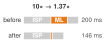
A faster model stage does not linearly speed up a camera pipeline.
Fallacy: Model optimization translates linearly to system speedup.
Amdahl’s Law40 establishes hard limits that the bottleneck principle (section 1.2.1) makes operational, where Strong scaling (Amdahl's Law) derives the strong-scaling form and works a speedup example at eight processors: \(\text{Speedup}_{\text{overall}} = \frac{1}{(1-p) + \frac{p}{s}}\) where \(p\) is the fraction of work that can be improved and \(s\) is the speedup of that fraction. Consider tapping the shutter on a smartphone camera. The image passes through 100 ms of signal processing (auto-exposure, white balance), 60 ms of ML scene classification, and 40 ms of postprocessing (tone mapping, HDR merge)—200 ms total. Optimizing the ML classifier to run 10× faster (6 ms instead of 60 ms) drops total time from 200 ms to —only 1.37× overall, not 10×. Even eliminating ML entirely \((s = \infty)\) achieves only 1.43× speedup, because the remaining 70 percent of the pipeline is untouched. Effective optimization requires profiling the entire pipeline and addressing bottlenecks systematically, because system performance depends on the slowest unoptimized stage.
40 Amdahl’s law: Formalized by Amdahl (1967) for multiprocessor scaling, this principle applies directly to ML deployment pipelines where the model is only one stage among many. In this camera pipeline example, ML inference is 60 ms of 200 ms; even a 100\(\times\) model speedup yields only about 1.4–2× end-to-end improvement because the rest of the pipeline is unchanged. Teams that benchmark model latency in isolation systematically overestimate deployment gains.
Amdahl, Gene M. 1967. “Validity of the Single Processor Approach to Achieving Large Scale Computing Capabilities.” Proceedings of the April 18-20, 1967, Spring Joint Computer Conference on - AFIPS ’67 (Spring), AFIPS ’67 (spring), 483–85. https://doi.org/10.1145/1465482.1465560.
Pitfall: Assuming more training data always improves deployed model performance.
Three constraints limit data scaling benefits, as the workload archetypes in section 1.2 illustrate. First, model capacity can limit what additional data contributes. Second, data quality can outweigh quantity because mislabeled examples and misleading patterns degrade performance. Third, deployment distribution matters: in-domain data can outperform much larger out-of-domain datasets.
Fallacy: One model binary can serve every edge hardware target efficiently.
Teams build a single model artifact and deploy it identically to every target device, treating deployment as a packaging step rather than an optimization opportunity. In practice, hardware-specific optimizations can yield substantial efficiency gains that generic binaries cannot capture. An INT8 model running on a device with a dedicated Neural Processing Unit (NPU) can achieve higher throughput per watt than the same model running in FP32 on a general-purpose CPU, because the NPU’s fixed-function INT8 datapaths avoid the energy overhead of floating-point arithmetic. Similarly, operator fusion (combining adjacent operations so intermediate tensors are not written back to memory) and memory layout tuning for a specific accelerator’s cache hierarchy can reduce inference latency without changing the model’s weights. As the deployment paradigm analysis in Deployment Paradigm Framework establishes, each paradigm imposes distinct hardware constraints; a model binary optimized for an Arm Cortex-A78 will underutilize the matrix acceleration units on a device equipped with an Arm Ethos-U NPU. Teams that skip per-target optimization either waste battery life on mobile devices or fail to meet latency SLAs on edge hardware, forcing costly postdeployment remediation. A generic artifact can remain a portability baseline, but profiling on the production runtime, delegate, memory hierarchy, and thermal envelope must determine whether it is acceptable, inefficient, or fundamentally mismatched.
Self-Check: Question
A smartphone camera pipeline takes 200 ms total: 100 ms for the image signal processor (ISP), 60 ms for ML scene classification, and 40 ms for postprocessing. If an engineering team optimizes the ML model to run \(10\times\) faster (reducing ML time from 60 ms to 6 ms), what is the overall system-level speedup?
- \(10.00\times\) speedup
- \(1.37\times\) speedup
- \(5.50\times\) speedup
- \(0.73\times\) speedup (system becomes slower)
Why does deploying a single generic FP32 model binary across diverse edge devices (e.g., Arm CPU, Apple Neural Engine, and Google Coral Edge TPU) result in suboptimal efficiency compared to per-target compilation?
- Generic model binaries violate cryptographic signatures required by PCI Express buses.
- Floating-point operations are mathematically undefined on mobile CPUs.
- Generic binaries cannot exploit hardware-specific operator fusion, dedicated fixed-point INT8 matrix datapaths, or accelerator-specific on-chip SRAM memory tiling.
- The operating system automatically deletes untuned model weights to prevent memory fragmentation.
Why does choosing an on-premises edge deployment solely because its hardware amortizes to a lower monthly compute cost than a cloud VM often result in a higher Total Cost of Ownership (TCO)?
Increasing the quantity of training data is guaranteed to continuously improve deployed model performance regardless of model capacity, label noise, or domain distribution shift.
What is operator fusion in ML compilers, and how does it optimize memory-bound inference pipelines?
Summary
ML systems engineering is governed by the physical reality that every deployment target enforces a distinct hardware contract. The iron law of ML systems (\(T = \frac{D_{\text{vol}}}{\text{BW}} + \frac{O}{R_{\text{peak}} \cdot \eta_{\text{hw}}} + L_{\text{lat}}\)) unifies these physical limits into a single execution model: propagation delay contributes fixed latency (\(L_{\text{lat}}\)), the memory wall bounds data movement (\(D_{\text{vol}}/\text{BW}\)), and thermal power budgets cap sustained compute. Across cloud, edge, mobile, and TinyML tiers, the categorical power envelope from megawatts to milliwatts spans nine orders of magnitude, while representative systems occupy narrower ranges within it.
By applying the bottleneck principle to workload archetypes, engineers determine whether a model’s latency is dominated by compute efficiency, memory bandwidth, or network transit before committing to single-node or hybrid architectures. The quantitative trade-offs (table 13) and systematic decision framework (figure 11) developed in this chapter establish the physical baselines that govern all downstream decisions in model compression, data pipeline design, and high-performance serving.
Key Takeaways: Same model, different engineering
- Physical constraints define feasibility: Speed of light (~36 ms cross-country round-trip), power wall, memory wall, and latency budgets create hard boundaries that engineering cannot overcome, only navigate.
- Identify bottlenecks before optimizing: The same model is compute bound in training but memory bound in inference. The iron law and bottleneck principle pinpoint which constraint dominates; optimizing the wrong term yields zero speedup.
- Workload archetypes determine deployment feasibility: A Compute Beast such as large-scale image-model training often needs cloud-scale resources; a Tiny Constraint such as keyword spotting requires microcontroller efficiency. The same optimization strategy cannot serve both; engineers must match the workload archetype to the deployment paradigm.
- Deployment power spans nine orders: Cloud data-center infrastructure operates at megawatt scale, while TinyML systems target milliwatts. This gap enables entirely different application classes rather than representing a limitation.
- Hybrid architectures are prevalent in production systems: Voice assistants span TinyML (wake-word), mobile (speech-to-text), and cloud (language understanding). When one paradigm does not suffice, integration patterns (train-serve split, hierarchical processing, progressive deployment) formalize how paradigms combine.
- System-level speedup obeys Amdahl’s Law, not model-level gains: In the worked camera pipeline, a 10\(\times\) faster model yields only 1.37\(\times\) system speedup when ML accounts for 30 percent of the pipeline. Profile the full system before optimizing any component.
- Deployment begins a feedback loop: Live data can diverge from training conditions while code and weights stay fixed, so monitoring and bounded operational exposure are part of the system architecture.
Deployment paradigms are not arbitrary design preferences; they are continuous operational regions dictated by physical laws. Selecting a deployment target changes which term of the iron law is most likely to bind: data-center training can push against peak compute (\(O/R_{\text{peak}}\)), mobile inference can collide with memory bandwidth (\(D_{\text{vol}}/\text{BW}\)), and remote real-time inference can be constrained by propagation delay (\(L_{\text{lat}}\)). Systems engineering begins by measuring that binding constraint. Optimizing model architecture or software runtimes without respecting the underlying hardware contract produces fragile systems that fail under real-world operational pressure.
What’s Next: From theory to process
While the physical constraints and decision framework established in section 1.8.2 define where an ML system can physically execute, physical feasibility alone does not guarantee operational success over time. As demonstrated by Zillow’s $304 million write-down (Zillow Group 2021), deploying models into production requires containing forecast uncertainty and managing operational risk across the software lifecycle. ML Workflow introduces the ML development lifecycle, the systematic engineering process that carries a system from problem formulation through deployment, monitoring, and maintenance.
Zillow Group. 2021. Zillow Group Reports Third-Quarter 2021 Financial Results and Shares Plan to Wind down Zillow Offers Operations. Investor Relations Press Release.
Self-Check: Question
Which summary statement best captures the core thesis of ML systems engineering regarding deployment paradigms?
- Software compilers have eliminated hardware differences, making any model executable on any hardware platform with identical efficiency.
- Model accuracy on standard benchmark datasets is the sole determinant of whether a system succeeds in production.
- Cloud computing is always the optimal deployment target because network bandwidth expands faster than processor compute capacity.
- Constraints drive architecture: permanent physical boundaries (the speed of light, thermodynamics, and memory signaling) partition deployment into distinct operating regimes, making deployment a first-order co-design problem across Data, Algorithm, and Machine.
Summarize how the iron law of ML systems helps engineers avoid wasted optimization effort during model development and deployment.
In ML systems engineering, successful deployment of a trained model represents the completion of the engineering task, because verified model weights maintain static accuracy indefinitely.
Self-Check Answers
Self-Check: Answer
A safety-critical autonomous braking system requires an end-to-end decision latency budget of 10 ms. A cloud data center is located 1,500 km away. Given that light travels through optical fiber at approximately \(200{,}000\text{ km/s}\), why is offloading inference to this cloud data center physically impossible?
- The cloud server queue latency always adds at least 25 ms regardless of server load.
- The speed of light in fiber allows a round trip in 5 ms, but serialization of model weights requires 15 ms.
- The minimum speed-of-light round-trip propagation time alone is 15 ms, consuming the entire 10 ms budget before compute begins.
- Wireless transmission protocols require a minimum 50 ms handshake before transmitting sensor packets.
Answer: The correct answer is C. The minimum round-trip propagation time over optical fiber is \(\frac{2 \times 1{,}500\text{ km}}{200{,}000\text{ km/s}} = 0.015\text{ s} = 15\text{ ms}\). This propagation delay alone exceeds the 10 ms budget by 5 ms before accounting for network routing, packet queuing, or model inference. The option citing a fixed 25 ms server queue latency confuses operational queuing with an invariant physical floor. The option claiming a 5 ms round trip miscalculates the distance-speed formula. The option attributing the failure to wireless handshakes references protocol overhead rather than the primary speed-of-light constraint.
Learning Objective: Calculate the physical latency floor imposed by the speed of light in optical fiber for distributed ML workloads.
Under dynamic CMOS power scaling where supply voltage scales proportionally with clock frequency (\(V \propto f\)), doubling the processor clock frequency increases dynamic power dissipation by a factor of 8 (\(f^3\)).
Answer: True. Dynamic CMOS power follows \(\text{Power} \propto C \cdot V^2 \cdot f\). When supply voltage \(V\) must scale proportionally with frequency \(f\) to support faster switching, substituting \(V \propto f\) yields \(\text{Power} \propto C \cdot f^3\). Consequently, doubling clock frequency (\(2\times\)) results in an \(8\times\) (\(2^3\)) increase in dynamic power, which explains why frequency scaling stalled when Dennard scaling broke down.
Learning Objective: Explain the cubic relationship between clock frequency and dynamic power in CMOS circuits and its impact on hardware scaling.
How does the memory wall manifest in modern computing hardware according to the historical growth rates of compute capacity versus memory bandwidth?
- Memory bandwidth doubles every 18 months while compute throughput increases by only 20% annually, causing compute starvation.
- Both compute throughput and memory bandwidth grow at identical 60% annual rates, but memory capacity limits model size.
- Processors have reached absolute thermal limits while memory signaling energy has dropped to near-zero levels.
- Compute capacity historically doubles roughly every 18 months (~60% annually), whereas memory bandwidth grows by only ~20% annually, causing the compute-to-bandwidth gap to widen compounding over time.
Answer: The correct answer is D. The memory wall is defined by the widening gap between compute growth (doubling roughly every 18 months, ~60% annual growth) and memory bandwidth growth (~20% annual growth), yielding a growth factor ratio of approximately \(\frac{1.6}{1.2} \approx 1.33\). This divergence makes data movement an increasingly dominant bottleneck across successive hardware generations. The option reversing compute and memory bandwidth growth contradicts historical scaling trends. The option claiming identical growth rates ignores the core definition of the memory wall. The option claiming memory signaling energy has dropped to near zero contradicts the physics of memory bus signaling.
Learning Objective: Analyze the quantitative divergence between processor compute growth and memory bandwidth growth that creates the memory wall.
What causes thermal throttling on passively cooled mobile devices running sustained ML inference, and how does it affect continuous model execution?
Answer: Passively cooled mobile devices have a limited thermal dissipation capacity (typically 2–5 W TDP). When sustained ML computation generates heat faster than the chassis can dissipate it, the internal temperature rises until it reaches the hardware thermal trip point (e.g., 80 °C). The operating system then throttles clock frequencies and duty cycles to protect the hardware, which can cause frame rates and inference throughput to drop precipitously (e.g., from 60 FPS down to 15 FPS).
Learning Objective: Evaluate the thermal throttling mechanism on mobile devices and its operational impact on sustained inference throughput.
The historical scaling relationship under which shrinking MOSFET transistor dimensions allowed reducing voltage and current while keeping power density constant is known as ____ scaling.
Answer: Dennard. Dennard scaling (formulated by Robert Dennard in 1974) held that as transistors shrank, power density remained constant because operating voltage and current scaled downward proportionally. Its breakdown in the mid-2000s ended free clock frequency scaling and forced the computing industry toward multicore parallelism and domain-specific accelerators.
Learning Objective: Explain the transistor power-scaling law whose breakdown led to domain-specific ML accelerators.
Self-Check: Answer
When analyzing ML system performance, when should an engineer apply the additive form of the iron law (\(T = \frac{D_{\text{vol}}}{\text{BW}} + \frac{O}{R_{\text{peak}} \cdot \eta_{\text{hw}}} + L_{\text{lat}}\)) versus the bottleneck principle’s max form (\(T = \max\left(\frac{D_{\text{vol}}}{\text{BW}}, \frac{O}{R_{\text{peak}} \cdot \eta_{\text{hw}}}, T_{\text{network}}\right) + L_{\text{lat}}\))?
- Use the additive form for single-task, serialized latency, and the max form for pipelined, steady-state throughput where computation and data prefetching overlap.
- Use the additive form exclusively for cloud workloads, and the max form exclusively for microcontroller TinyML workloads.
- Use the additive form when batch size is greater than 128, and the max form when batch size equals 1.
- Use the additive form during model training only, and the max form during on-device model quantization.
Answer: The correct answer is A. The additive form models isolated single-task execution where data movement, computation, and overhead occur sequentially and their latencies sum up directly. The max form applies to pipelined, steady-state execution where modern hardware overlaps data movement (prefetching batch \(n+1\)) with computation (processing batch \(n\)), making the slowest pipelined stage the bounding throughput bottleneck. The option dividing the formulas by deployment tier (cloud vs. TinyML) incorrectly couples execution flow with device location. The choice associating the additive form with large batch sizes reverses the intuition: batching often enables pipelined overlap. The option restricting the formulas to training versus quantization confuses performance modeling with workflow stages.
Learning Objective: Apply the iron law and bottleneck principle to distinguish between serialized task latency and pipelined throughput bounds.
Which pairing correctly matches a workload archetype to its dominant physical bottleneck and canonical lighthouse model?
- Compute Beast \(\rightarrow\) dominated by irregular table lookups and cache misses \(\rightarrow\) DLRM
- Bandwidth Hog \(\rightarrow\) dominated by dense parameter streaming during autoregressive token decode \(\rightarrow\) GPT-2/Llama
- Sparse Scatter \(\rightarrow\) dominated by dense FLOP throughput at high arithmetic intensity \(\rightarrow\) ResNet-50
- Tiny Constraint \(\rightarrow\) dominated by petabyte-scale distributed training \(\rightarrow\) Keyword Spotting (KWS)
Answer: The correct answer is B. Bandwidth Hog workloads, exemplified by autoregressive language models such as GPT-2 and Llama, perform sequential token decoding where generating each token requires streaming large parameter matrices through memory, making memory bandwidth (\(\text{BW}\)) the primary bottleneck. The option pairing Compute Beast with DLRM confuses dense arithmetic with sparse embedding lookups. The option pairing Sparse Scatter with ResNet-50 misclassifies a dense convolution model as an irregular lookup table. The option pairing Tiny Constraint with petabyte-scale distributed training contradicts the kilobyte memory and milliwatt power constraints of TinyML.
Learning Objective: Classify ML workloads into archetypes based on their dominant iron law bottlenecks and reference lighthouse models.
In a battery-powered IoT sensor, why does sending raw sensor data (e.g., 1 MB audio) over a cellular or Wi-Fi radio often consume significantly more energy than running local neural network inference (e.g., MobileNetV2)?
Answer: Radio transmission of raw data typically requires 500–1000 mJ per megabyte over wireless links (e.g., 5G/Wi-Fi), whereas running a compact quantized model like MobileNetV2 on an energy-efficient on-device processor requires only tens of millijoules (e.g., ~50 mJ) per inference. Because transmission energy is hundreds of times higher than local compute energy for the same payload, battery-constrained sensors achieve much longer battery life by processing data locally and transmitting only compact detection summaries.
Learning Objective: Calculate and compare the energy trade-off between wireless data transmission and local neural processing.
**Order the steps of the hierarchical deployment feasibility evaluation for the Smart Doorbell scenario from initial resource check to latency verification:
- Verify Level 1 resource capacity fit (confirm model weights and activations fit in microcontroller SRAM/Flash)
- Define application mission targets (specify model task, accuracy target, and real-time SLA budget)
- Verify Level 2 timing constraints (evaluate per-inference execution latency against the strict interaction SLA)
- Select deployment candidate platform and model archetype (match keyword spotter to ESP32-S3 microcontroller)**
Answer: The correct order is (2) Define application mission targets, (4) Select deployment candidate platform and model archetype, (1) Verify Level 1 resource capacity fit, and (3) Verify Level 2 timing constraints. Deployment feasibility must be evaluated hierarchically: first define the application SLA and task, then select candidate hardware and archetype, next confirm physical memory fit (Level 1 capacity check), and finally evaluate execution latency against the SLA budget (Level 2 timing check).
Learning Objective: Design a hierarchical constraint scorecard evaluation to determine deployment feasibility on embedded hardware.
An ML workload characterized by high arithmetic intensity where throughput is bounded by peak FLOP/s (\(R_{\text{peak}}\)) rather than memory bandwidth, such as dense convolutional neural network training, belongs to the ____ archetype.
Answer: Compute Beast. Compute Beast workloads perform many floating-point operations per byte of memory loaded (\(I = \text{FLOPs/byte}\)), ensuring that processor arithmetic units remain saturated and execution time is dominated by the compute term (\(O / (R_{\text{peak}} \cdot \eta_{\text{hw}})\)) of the iron law.
Learning Objective: Classify ML workloads exhibiting high arithmetic intensity into the Compute Beast archetype.
Self-Check: Answer
Why is single-image (batch=1) ResNet-50 inference memory-bound on both a high-end cloud accelerator (NVIDIA A100) and a mobile NPU (iPhone 15 Pro)?
- ResNet-50 contains dynamic control flow that causes branching stalls on SIMD execution units.
- Both platforms lack matrix multiplication coprocessors, forcing scalar CPU execution.
- At batch=1, model weights must be loaded from memory once per single image without weight reuse across batch items, keeping arithmetic intensity below each platform’s hardware balance point (\(R_{\text{peak}}/\text{BW}\)).
- The activations at batch=1 exceed the total high-bandwidth memory (HBM) and SRAM capacities of both devices.
Answer: The correct answer is C. For single-image inference (\(\text{batch}=1\)), the full model weight parameters must be fetched from memory to process a single sample. Because weights cannot be amortized across multiple samples in parallel, the effective arithmetic intensity (\(I = \text{FLOPs/byte}\)) is low and falls to the left of the roofline ridge point (\(R_{\text{peak}}/\text{BW}\)) on both the A100 and the mobile NPU, making memory bandwidth the limiting constraint on both chips. The option citing dynamic control flow is incorrect because ResNet-50 consists of regular static feedforward convolutions. The claim that both platforms lack matrix acceleration is false, as both feature specialized tensor cores / NPUs. The option claiming activations exceed memory capacity is false, as ResNet-50 activations at batch=1 require only a few megabytes.
Learning Objective: Analyze why single-batch inference is memory-bound across heterogeneous hardware platforms using the roofline model.
Why does a convolutional neural network (e.g., ResNet-50) shift from a compute-bound regime during cloud training to a memory-bound regime during single-sample (\(\text{batch}=1\)) edge inference?
Answer: During cloud training with large batch sizes (e.g., \(\text{batch}=256\)), loaded model weights are reused across hundreds of input samples in parallel, raising arithmetic intensity (\(I = \text{FLOPs/byte}\)) above the hardware balance point into the compute-bound regime. During single-sample inference (\(\text{batch}=1\)), the full set of model weights must be streamed from memory to process just one input without reuse, causing arithmetic intensity to plummet onto the memory-bandwidth-bound slope of the roofline.
Learning Objective: Explain how the dominant bottleneck shifts between compute-bound and memory-bound regimes across training and inference phases.
An ML service SLA guarantees a total end-to-end response time of 100 ms. The pipeline involves client preprocessing, a cross-region network RPC, model inference, and postprocessing. According to critical path latency principles, why will this system fail if a cross-region network call taking 120 ms is placed on the synchronous critical path?
- The ML framework compiler will refuse to lower the graph if network RPC operations are detected.
- Cross-region RPCs corrupt the numerical precision of FP16 tensors during serialization.
- A cross-region network call reduces the accelerator compute throughput (\(R_{\text{peak}}\)) by half.
- The critical path is the longest sequential chain of dependent operations; any single stage exceeding 100 ms guarantees the end-to-end SLA will be breached regardless of how fast all other stages execute.
Answer: The correct answer is D. In a synchronous pipeline, end-to-end latency is bounded below by the sum of sequential operations on the critical path. If an individual operation on the critical path requires 120 ms, the system latency is guaranteed to be at least 120 ms, violating the 100 ms budget before accounting for inference, preprocessing, or postprocessing. The options citing compiler lowering errors, tensor precision corruption, or halved accelerator throughput invent non-existent technical failures instead of applying critical-path analysis.
Learning Objective: Apply the critical path latency rule to evaluate end-to-end ML service level agreements.
What is the hardware balance point (or roofline ridge point) of an accelerator, and what does it tell an ML systems engineer about whether a workload will be compute-bound or memory-bound?
Answer: The hardware balance point is the ratio of peak arithmetic throughput to memory bandwidth (\(R_{\text{peak}} / \text{BW}\)), expressed in \(\text{FLOPs/byte}\). If a workload’s arithmetic intensity (\(I = \text{operations} / \text{bytes moved}\)) is greater than this balance point (\(I > R_{\text{peak}}/\text{BW}\)), the workload is compute-bound and limited by processor arithmetic capacity. If \(I < R_{\text{peak}}/\text{BW}\), the workload is memory-bound and limited by memory bandwidth, meaning buying more peak FLOP/s will provide zero speedup unless data movement is reduced.
Learning Objective: Calculate the hardware balance point and use it to classify workloads into compute-bound and memory-bound regimes.
In ML accelerator memory hierarchies, an L1 cache hit requires approximately 1 ns, whereas an uncached global DRAM read requires approximately 200–____ ns.
Answer: 500. Global memory access latency on GPUs and accelerators is roughly 200–500 ns, which is over two orders of magnitude slower than an L1 cache hit (~1 ns). This latency penalty is why accelerator kernels rely on memory coalescing, shared memory tiling, and massive thread parallelism to hide DRAM access latencies.
Learning Objective: Compare order-of-magnitude latencies across the memory hierarchy in modern ML accelerators.
Self-Check: Answer
Why does serving always-on voice assistant traffic (e.g., 1 billion devices issuing continuous audio queries) entirely in the cloud create an ‘infrastructure and economic wall’?
- The cloud approach would cost hundreds of millions of dollars annually and require dozens of dedicated data centers at peak hours, whereas on-device TinyML wake-word detection filters idle traffic for pennies per device.
- Cloud servers cannot execute transformer models with audio spectrogram inputs due to floating-point representation limits.
- Data privacy regulations in all jurisdictions make transmitting any encrypted audio to cloud servers illegal under all circumstances.
- Cloud network switches drop all audio packets exceeding 1 kHz sampling rates due to MTU size limits.
Answer: The correct answer is A. Continuous cloud-only voice processing for 1 billion devices would require tens of millions of daily GPU hours (~20+ dedicated data centers at peak waking hours) and hundreds of millions of dollars in annual cloud infrastructure costs. Layering a TinyML wake-word detector directly on the device enables always-on listening at sub-milliwatt power (<$0.01/device/year) and only engages higher-power speech recognition and cloud reasoning when a wake word is detected. The option claiming transformers cannot process audio spectrograms is factually false. The option asserting that transmitting encrypted audio is globally illegal misrepresents privacy regulations, which permit transmission with appropriate user consent and legal safeguards. The option alleging that network switches drop packets above 1 kHz fabricates an impossible networking rule.
Learning Objective: Analyze the infrastructure and economic scaling limits that prevent cloud-only processing for global-scale always-on voice assistants.
In a 3-year Total Cost of Ownership (TCO) comparison for an on-premises edge server deployment serving 1 million inferences per day, what is typically the largest component of the edge system’s annual cost?
- GPU hardware silicon purchase price amortized over 3 years
- DevOps engineering labor required to maintain, update, and manage on-premises edge infrastructure
- Electricity costs for running the server 24/7
- Dedicated server room air-conditioning and cooling overhead
Answer: The correct answer is B. In realistic edge server TCO modeling, engineering labor (e.g., 0.1 FTE DevOps support per server/site, totaling ~$15,000/year) accounts for roughly 60% of total annual edge expenses, far exceeding hardware CapEx (~$5,000/year), power (~$500/year), or cooling (~$150/year). Teams that focus solely on minimizing hardware purchase costs systematically underestimate the total cost of ownership. The choices identifying hardware amortization, electricity, or cooling as the dominant cost ignore the reality that personnel and operational maintenance dominate distributed on-premise infrastructure.
Learning Objective: Evaluate the cost components of edge vs. cloud TCO to identify the dominant role of operational labor.
What is the data gravity invariant in cloud ML, and why does it make moving multi-terabyte raw sensor datasets to the cloud economically and physically problematic?
Answer: The data gravity invariant states that as data volume (\(D_{\text{vol}}\)) grows, the cost and latency of moving data to compute (\(C_{\text{move}}(D_{\text{vol}})\)) eventually dominates the cost of moving compute to data (\(C_{\text{move}}(\text{Compute})\)). For massive sensor streams (such as hundreds of raw video feeds generating tens of gigabytes per second), the required network bandwidth exceeds uplink capacities and incurs exorbitant cloud ingest/egress costs, forcing computation to move to the edge.
Learning Objective: Explain the data gravity invariant and its implications for data-movement costs in cloud systems.
Under GDPR Article 17 (Right to Erasure), when a user requests deletion of their data, an organization is legally mandated to retrain from scratch every ML model that ever encountered that user’s training samples.
Answer: False. GDPR Article 17 provides a right to erasure across source data stores, derived feature pipelines, caches, and logs where specified grounds apply, but it is technology-neutral and does not prescribe retraining every trained model as the sole mandatory remediation. Organizations evaluate risk, data persistence, and technical measures appropriate to the system.
Learning Objective: Classify the operational and legal boundaries of data erasure regulations (GDPR) on deployed ML models.
**Order the steps of a hybrid voice assistant query pipeline from the initial acoustic trigger to user response:
- Run on-device speech-to-text (ASR) on a mobile NPU to convert speech to text tokens locally
- Transmit text tokens to cloud infrastructure for large language model reasoning and broad knowledge retrieval
- Always-on TinyML wake-word detector listens continuously on a sub-milliwatt dedicated core
- Send synthetic audio/text response back to the client device to render the answer to the user
- Detect trigger phrase (“Hey Assistant”) and wake the main application processor from sleep**
Answer: The correct order is (3) Always-on TinyML wake-word detector listens continuously on a sub-milliwatt dedicated core, (5) Detect trigger phrase and wake the main application processor, (1) Run on-device speech-to-text on mobile NPU, (2) Transmit text tokens to cloud infrastructure for reasoning, and (4) Send response back to the client device. This tiered architecture minimizes power by keeping the main processor asleep until a wake word is detected, protects privacy and latency with local ASR, and leverages cloud scale only for complex natural language queries.
Learning Objective: Design a tiered hybrid pipeline spanning TinyML, mobile NPU, and cloud infrastructure for voice assistant processing.
Self-Check: Answer
A manufacturing facility deploys 100 cameras recording uncompressed 1080p video (\(1920 \times 1080 \times 3\text{ bytes/pixel}\)) at 30 FPS. The factory has a dedicated 10 Gbps (~1.25 GB/s) fiber uplink. Why is streaming all raw video to a cloud ML server physically impossible?
- 1080p video frames contain interlaced scanlines that cloud GPUs cannot decompress.
- Fiber optic cables can only carry voice data, requiring microwave radio relays for video.
- The aggregate raw video data rate is approximately 18.7 GB/s, which exceeds the 1.25 GB/s uplink capacity by roughly 15-fold.
- Cloud object detection models require uncompressed video to be transmitted in 10-minute batched tar archives.
Answer: The correct answer is C. Each camera generates \(1920 \times 1080 \times 3 \times 30 \approx 186.6\text{ MB/s}\). Across 100 cameras, the aggregate data rate is \(18.66\text{ GB/s}\) (~18.7 GB/s). A 10 Gbps network provides a maximum theoretical bandwidth of \(\frac{10\text{ Gbps}}{8\text{ bits/byte}} = 1.25\text{ GB/s}\). The required traffic exceeds the network capacity by roughly \(15\times\), making cloud streaming physically impossible. Edge processing resolves this by detecting defects locally and transmitting only compact metadata events (~1 KB per event). The options alleging interlaced scanline incompatibilities, fiber cable restrictions to voice, or mandatory 10-minute tar archiving fabricate false technical constraints.
Learning Objective: Calculate aggregate sensor bandwidth demand and compare it against uplink limits to diagnose edge bandwidth bottlenecks.
An autonomous drone navigates at 60 FPS (16.7 ms per-frame budget) capturing uncompressed 4K frames (~24.9 MB per frame). The drone connects via a 100 Mbps uplink to a cloud server whose round-trip latency plus inference time is 110 ms. Applying the data locality invariant, what is the feasibility of offloading this obstacle avoidance system to the cloud?
- Feasible, because the cloud GPU computes inference in under 10 ms.
- Feasible, provided 5G network slicing is enabled on the drone modem.
- Infeasible, solely because cloud servers do not support drone telemetry protocols.
- Infeasible, because transmitting a 24.9 MB frame over a 100 Mbps link requires ~2,000 ms, causing the complete remote path (~2,110 ms) to violate the 16.7 ms frame deadline by over two orders of magnitude.
Answer: The correct answer is D. Under the data locality invariant, the complete remote path time is \(T_{\text{remote}} = \frac{D_{\text{vol}}}{\text{BW}_{\text{network}}} + L_{\text{lat,network}} + T_{\text{compute,remote}}\). Transmitting \(24.9\text{ MB} = 199.2\text{ Mbits}\) over a \(100\text{ Mbps}\) uplink requires \(\frac{199.2}{100} \approx 1.992\text{ s} \approx 2{,}000\text{ ms}\). Adding the 110 ms network/compute delay yields \(T_{\text{remote}} \approx 2{,}110\text{ ms}\), vastly exceeding the 16.7 ms per-frame budget. Because transmission time alone dominates, cloud offloading is completely infeasible. The options claiming feasibility ignore the two-second transmission bottleneck. The option blaming telemetry protocols misses the fundamental bandwidth-latency physics.
Learning Objective: Apply the data locality invariant equation to determine whether an application must run locally at the edge.
Why cannot high-bandwidth wireless networking technologies (such as 5G or 6G) eliminate the need for edge ML in tight real-time control loops (\(<10\text{ ms}\))?
Answer: While 5G and 6G technologies dramatically increase network bandwidth (\(\text{BW}_{\text{network}}\)) and reduce data transmission serialization time, they cannot alter the speed of light in optical fiber or eliminate physical geographic routing delays and protocol overhead (\(L_{\text{lat,network}}\)). For tight real-time control loops (\(<10\text{ ms}\)), physical round-trip propagation over geographic distances alone can consume the entire latency budget before any computation begins, making local edge execution physically mandatory.
Learning Objective: Evaluate why high-bandwidth cellular networks (5G/6G) cannot eliminate the need for edge ML in sub-10 ms control loops.
When sizing edge accelerators for a retail store deployment requiring 7.2 TOPS of sustained INT8 throughput, why is it inadequate to select a single accelerator rated at 8 TOPS peak datasheet throughput?
Answer: Hardware datasheets publish peak theoretical throughput (\(R_{\text{peak}}\)), but real-world sustained workloads encounter thermal limits, memory bandwidth bottlenecks, and software overhead, typically achieving only a derated fraction (e.g., 50% derating, yielding ~4 TOPS sustained from an 8 TOPS peak chip). To reliably deliver 7.2 TOPS sustained throughput with sufficient headroom, sizing must be based on sustained performance, requiring multiple sharded boards (e.g., two 8 TOPS peak boards delivering 8 TOPS sustained) or a higher-tier accelerator.
Learning Objective: Calculate sustained accelerator requirements for edge deployments using hardware derating factors.
In industrial IoT manufacturing systems (Industry 4.0), the complete ML control loop latency (\(L_{\text{lat}}\)) must be strictly shorter than the ____ of the physical machinery it governs (such as a 16.7 ms window for a 60 Hz welding robot).
Answer: sampling interval (or control cycle time / sampling period). In real-time cyber-physical systems, sensor-actuator feedback loops require that sensing, model inference, and actuation complete within the physical process’s sampling interval (e.g., 16.7 ms for a 60 Hz process), otherwise the system fails to prevent defects or safety violations.
Learning Objective: Evaluate the control loop timing constraints governing real-time industrial IoT ML deployments.
Self-Check: Answer
How do the battery tax** and the thermal wall differ as physical constraints on mobile ML systems?**
- The battery tax is an energy budget problem bounding total operations over time (\(\int \text{Power} \cdot dt\)), whereas the thermal wall is a heat dissipation ceiling bounding instantaneous sustained power (\(\text{Power} \le 2\text{--}5\text{ W}\)) regardless of battery size.
- The battery tax applies only to iOS devices, while the thermal wall applies only to Android devices.
- The battery tax can be resolved by lowering clock frequency, but the thermal wall requires increasing the clock frequency to finish calculations faster.
- The battery tax represents static memory leakage in SRAM, while the thermal wall represents network transmission power in 5G modems.
Answer: The correct answer is A. The battery tax represents the depletion of finite electrochemical energy (\(E = P \cdot t\)) over a full day, meaning a model running continuously draws down the daily battery budget. The thermal wall represents the maximum rate of heat that a phone’s passive chassis can continuously dissipate (typically 2–5 W TDP). Adding a larger battery extends runtime but cannot prevent thermal throttling if the workload exceeds the thermal dissipation ceiling. The option dividing the constraints by mobile operating system is factually baseless. The option suggesting higher clock frequencies to beat the thermal wall violates the cubic power law (\(\text{Power} \propto f^3\)). The option conflating the terms with SRAM leakage and modem power misdefines both concepts.
Learning Objective: Compare the battery tax and the thermal wall as distinct energy and thermodynamic constraints in mobile ML.
Why does deploying a mobile computational photography feature (such as Portrait Mode or Night Mode) present a pipeline scheduling challenge rather than a single-model optimization problem?
- Mobile cameras can only run one neural network per battery charge cycle.
- The feature executes a multi-stage pipeline (depth estimation, semantic segmentation, alignment, and HDR tone mapping) that must all complete within a perceived shutter delay while sharing a 2–5 W thermal budget across CPU, GPU, and NPU.
- Computational photography models cannot use quantized INT8 representations due to mathematical rounding artifacts in lens optics.
- Camera image signal processors (ISPs) operate asynchronously from the operating system and reject all external ML tensor inputs.
Answer: The correct answer is B. Mobile computational photography does not rely on a single isolated model; it executes a sequence of specialized real-time models (such as depth estimation, segmentation, and denoising) alongside the ISP. All stages must execute within the user’s perceived shutter delay (tens to hundreds of milliseconds) while sharing the phone’s tight 2–5 W thermal envelope across heterogeneous SoC cores (CPU, GPU, NPU) without triggering thermal throttling. The option claiming one network per charge cycle is absurd. The option claiming optics prevent INT8 quantization is false, as mobile vision pipelines routinely use quantized models. The option claiming ISPs reject ML tensor inputs misrepresents modern mobile SoC architectures where ISPs and NPUs share memory.
Learning Objective: Analyze the system scheduling and thermal constraints of multi-stage computational photography pipelines on mobile SoCs.
Why does deploying an unoptimized desktop-trained vision model (such as an FP32 ResNet-50 pipeline) directly onto a mobile device frequently fail, even when the model’s FP32 weights (~98 MB) appear smaller than the phone’s total RAM?
Answer: While the raw FP32 weights are ~98 MB, a complete desktop pipeline requires gigabytes of memory once intermediate activation tensors, input/output preprocessing buffers, runtime framework overhead, and batch buffers are allocated. Furthermore, unoptimized desktop models execute billions of FLOPs (e.g., 4.1 GFLOPs per image) using unsupported float operations or desktop-specific layers, exceeding the mobile device’s 2–5 W thermal envelope and causing thermal throttling or out-of-memory crashes.
Learning Objective: Analyze why desktop-trained models fail on mobile devices due to activation memory, thermal budgets, and unsupported operations.
Running biometric matching (such as Face ID) inside a dedicated on-device Secure Enclave reduces data disclosure risks by keeping mathematical representations isolated in encrypted hardware, but it does not automatically eliminate all security or privacy risks without rigorous end-to-end system design.
Answer: True. Hardware isolation mechanisms like the Secure Enclave restrict biometric mathematical representations to dedicated encrypted memory on-device, preventing remote transmission and unauthorized operating system access. However, overall system security and privacy still depend on the complete threat model, authentication policies, and software implementation.
Learning Objective: Evaluate how dedicated hardware enclaves (e.g., Secure Enclave) provide biometric privacy while recognizing holistic system threat models.
**Order the sequence of events that occurs when an unoptimized 12 W deep learning model runs continuously on a passively cooled 3 W smartphone SoC:
- The device temperature rises rapidly (e.g., at ~1 °C per second) as power dissipation exceeds passive cooling capacity
- The unoptimized model launches at full burst performance (e.g., 100 FPS) drawing 12 W of active compute power
- Operating system and hardware thermal controllers engage thermal throttling, reducing clock frequencies and duty cycles
- The internal SoC junction temperature reaches the critical thermal trip point (e.g., 80 °C)
- Sustained inference throughput drops precipitously (e.g., from 100 FPS to 30 FPS) to stabilize power within the 3 W TDP envelope**
Answer: The correct order is (2) The unoptimized model launches at full burst performance drawing 12 W, (1) The device temperature rises rapidly as power exceeds passive cooling capacity, (4) The internal SoC temperature reaches the critical thermal trip point, (3) OS and hardware engage thermal throttling, and (5) Sustained inference throughput drops precipitously to stabilize within the 3 W TDP envelope. This sequence illustrates why peak burst benchmarks on mobile devices do not reflect sustained real-world performance.
Learning Objective: Explain the physical sequence of events during mobile thermal throttling under unoptimized compute workloads.
Self-Check: Answer
Comparing a dedicated TinyML keyword spotting model (~\(10\ \mu\text{J}\) per inference) to a cloud foundation model query (~\(1\text{ kJ}\) per inference), by approximately what factor does energy consumption per inference differ?
- Approximately \(100\times\) (2 orders of magnitude)
- Approximately \(10{,}000\times\) (4 orders of magnitude)
- Approximately \(100{,}000{,}000\times\) (\(10^8\), 8 orders of magnitude)
- Approximately \(10^{14}\times\) (14 orders of magnitude)
Answer: The correct answer is C. The energy ratio between a cloud LLM query (\(1\text{ kJ} = 10^3\text{ J}\)) and an always-on TinyML keyword spotting inference (\(10\ \mu\text{J} = 10^{-5}\text{ J}\)) is \(\frac{10^3\text{ J}}{10^{-5}\text{ J}} = 10^8 = 100{,}000{,}000\times\) (eight orders of magnitude). This vast efficiency gap enables TinyML sensors to operate for years on a coin-cell battery or milliwatt energy harvesters. The options citing 2 orders (\(100\times\)) or 4 orders (\(10{,}000\times\)) severely underestimate the energy gap between cloud data centers and microcontrollers. The option citing 14 orders (\(10^{14}\)) overstates the ratio.
Learning Objective: Calculate the multi-order-of-magnitude energy efficiency gap between TinyML sensing and cloud LLM queries.
Why are microcontroller TinyML devices predominantly restricted to inference-only execution rather than full in-situ backpropagation training?
- Microcontrollers use flash memory which permanently locks all transistor gates against state changes.
- Backpropagation requires double-precision FP64 floating-point arithmetic which is mathematically impossible on 32-bit cores.
- The speed of light inside microcontroller silicon is too slow to support backward gradient propagation.
- Standard backpropagation requires storing intermediate activation tensors from every forward layer until the backward pass executes, which quickly exceeds the microcontroller’s 256 KB–2 MB on-chip SRAM capacity.
Answer: The correct answer is D. During inference, intermediate activation buffers can be discarded and overwritten as soon as the subsequent layer completes execution. In contrast, standard backpropagation training requires retaining intermediate activations from all layers in memory throughout the forward pass to compute weight gradients during the backward pass, scaling memory linearly with model depth. With only 256 KB to 2 MB of on-chip SRAM and no virtual memory, microcontrollers cannot hold these training activations unless specialized parameter-efficient techniques (such as TinyTL, which freezes weights and updates only bias vectors) are applied. The choices claiming flash memory locks transistors, FP64 is mathematically impossible on 32-bit cores, or speed of light prevents gradient calculation are all scientifically absurd.
Learning Objective: Explain why activation memory retention during the backward pass prevents full on-device training on microcontrollers.
Why is the 1 mW average power threshold considered a transformative milestone in TinyML system deployment?
Answer: Operating at or below an average power draw of 1 mW allows embedded devices to be powered indefinitely by ambient energy harvesting (such as small thumbnail-sized solar cells, thermoelectric generators on warm pipes, or RF energy harvesters). This shifts the deployment model from a battery-limited lifespan requiring periodic manual battery replacement to a ‘deploy and forget’ paradigm, enabling ubiquitous sensing across millions of unattended physical assets.
Learning Objective: Justify how achieving a sub-1 mW power envelope enables perpetual operation via ambient energy harvesting.
Why is it a fallacy to treat TinyML as merely ‘scaled-down mobile ML’ that can be addressed simply by applying standard INT8 post-training quantization?
Answer: TinyML operates under qualitative discontinuities rather than minor quantitative scale-downs: microcontrollers possess a 10,000-fold smaller memory budget (kilobytes of on-chip SRAM vs. gigabytes of DRAM) and a 1,000-fold lower power envelope (milliwatts vs. watts). Quantizing a standard mobile model from FP32 to INT8 yields only a \(4\times\) size reduction, which fails to fit multi-megabyte models into a 64–256 KB microcontroller SRAM budget, requiring entirely different lightweight architectures, fixed-point operations, and bare-metal runtime execution.
Learning Objective: Explain the qualitative architectural discontinuities in memory and power that differentiate TinyML from mobile ML.
The power management paradigm in which a battery-less or energy-harvesting microcontroller sleeps in ultra-low-power states and wakes periodically to perform inference before energy reserves deplete is called ____ computing.
Answer: intermittent (or duty-cycled). Intermittent computing enables microcontrollers powered by tiny batteries (like CR2032 coin cells) or ambient energy harvesters to achieve multi-year lifespans by keeping average active power consumption in the microwatt to milliwatt regime.
Learning Objective: Explain the operational role of intermittent computing in energy-harvesting TinyML deployments.
Self-Check: Answer
In the four-layer deployment screening decision framework, why is the Privacy** layer evaluated first, followed by Latency, Compute Demand, and Cost?**
- The layers are ordered by how rapidly a hard constraint can completely invalidate an architecture: legal/privacy rules may forbid remote transmission entirely, physical latency limits can make cloud offload impossible, compute demands eliminate undersized devices, and cost compares the remaining feasible survivors.
- Privacy is the easiest parameter to optimize in software using compiler flags, whereas cost cannot be calculated until after deployment.
- Cloud providers require privacy agreements before allowing access to GPU instances.
- The framework is ordered purely alphabetically based on traditional software engineering conventions.
Answer: The correct answer is A. The decision framework sequences evaluation gates by their ability to disqualify candidates immediately: privacy and regulatory mandates can strictly prohibit sending raw data off-premises; physical latency constraints (e.g., speed of light) can make remote execution physically incapable of meeting real-time SLAs; compute/memory capacity determines whether candidate hardware can fit the workload; and finally, cost and operational complexity compare the feasible options. The option claiming privacy is a compiler flag trivializes regulatory compliance. The option alleging cloud GPU access requires upfront privacy agreements confuses commercial terms with architectural screening. The choice claiming alphabetical ordering is factually false.
Learning Objective: Apply the sequential screening logic of the four-layer deployment decision framework.
An autonomous vehicle travels at 100 km/h (~27.8 m/s). An emergency pedestrian detection system evaluates two architectures: (1) an automotive Edge ML accelerator with a 15 ms local detection latency, and (2) a Cloud ML server with 115 ms total latency (100 ms network RTT + 15 ms compute). How much additional distance does the vehicle travel before braking begins if the cloud architecture is used?
- 0.28 meters
- Approximately 2.8 meters
- Approximately 28 meters
- Exactly 100 meters
Answer: The correct answer is B. At \(100\text{ km/h}\), the vehicle travels at \(\frac{100}{3.6} \approx 27.78\text{ m/s}\). The cloud architecture adds $100 = 0.1 of network round-trip delay. The additional distance traveled during this delay is \(27.78\text{ m/s} \times 0.1\text{ s} \approx 2.78\text{ m}\) (~2.8 meters). In safety-critical emergency braking, a 2.8-meter delay can be the difference between stopping safely and a catastrophic collision, demonstrating why hard real-time latency budgets eliminate cloud offload. The options calculating 0.28 m, 28 m, or 100 m represent arithmetic scaling errors.
Learning Objective: Calculate the physical displacement and safety consequences of network latency in autonomous vehicle braking systems.
What is the complexity tax** in ML systems engineering, and when is a simple heuristic (e.g., rule-based logic or regular expressions) superior to a deep learning pipeline?**
Answer: The complexity tax refers to the extensive hidden operational overhead that an ML system introduces beyond its core model code, including data validation pipelines, continuous monitoring, retraining infrastructure, GPU dependencies, and model drift management. When an ML model provides only marginal accuracy gains (e.g., 95% vs. 90%) over a simple heuristic, but demands a massive increase in code maintenance and operational debugging (e.g., 40 hours/month vs. 1 hour/month), the simpler heuristic is the superior systems engineering choice.
Learning Objective: Evaluate the complexity tax of deploying machine learning systems compared to traditional software heuristics.
In ML systems engineering, selecting a deployment paradigm based solely on benchmark model accuracy is a sound practice because hardware infrastructure can always be scaled to meet application constraints later.
Answer: False. Selecting a deployment paradigm based solely on accuracy without evaluating physical constraints (latency floors, battery life, thermal ceilings, memory budgets, network availability) leads to deployment failures. A high-accuracy cloud model is useless if network delay violates an emergency response SLA, and an edge model that drains a mobile battery in minutes fails regardless of benchmark accuracy. Systems constraints must be co-designed upfront.
Learning Objective: Evaluate the critical pitfall of selecting deployment paradigms based on model accuracy alone.
What is the Total Cost of Ownership (TCO) calculation, and why must ML architects evaluate TCO rather than hardware purchase price or cloud VM hourly rates alone when selecting a deployment paradigm?
Answer: Total Cost of Ownership (TCO) encompasses all direct and indirect expenses over a system’s multi-year operational lifetime, including hardware CapEx, recurring energy and cooling costs, network bandwidth/egress, reliability engineering, software maintenance, and DevOps labor. Focusing solely on hardware purchase price or cloud VM rental rates leads to false economies, because operational overhead and engineering labor often constitute the vast majority (e.g., ~60%) of total system costs.
Learning Objective: Evaluate how Total Cost of Ownership (TCO) analysis prevents misleading paradigm selection based on compute list prices alone.
Self-Check: Answer
A smart agriculture system deploys soil moisture sensors on microcontrollers performing local anomaly detection, local gateway edge servers that aggregate sensor feeds across crop fields to trigger automated irrigation valves, and a central cloud system that aggregates regional data for seasonal crop yield forecasting. Which hybrid ML integration pattern does this architecture exemplify?
- Pure Train-Serve Split
- Monolithic Cloud Offload
- Hierarchical Processing
- Linear Single-Node Pipelining
Answer: The correct answer is C. Hierarchical Processing organizes data and decision-making across computational tiers based on timescale and capability: TinyML nodes perform millisecond-level local anomaly detection, edge gateways aggregate multi-sensor data for sub-second local irrigation actuation, and cloud infrastructure handles macro-scale long-term analytics. Train-Serve Split focuses specifically on separating centralized training from distributed serving. Monolithic Cloud Offload routes all raw sensor telemetry directly to the cloud without intermediate edge intelligence. Linear Single-Node Pipelining refers to overlapping compute within a single host.
Learning Objective: Classify real-world multi-tier deployments into canonical hybrid ML integration patterns.
What is the primary operational failure risk in a hybrid ML system where preprocessing and feature extraction are split between client devices (mobile/edge) and centralized cloud servers?
- Transistors in edge devices reverse polarity when receiving cloud RPC payloads.
- The speed of light in optical fiber decreases proportionally with the number of connected edge clients.
- Edge devices become unable to allocate floating-point registers during network handshakes.
- Training-serving skew, where slight discrepancies in feature extraction logic, library versions, or numerical precision between the edge client and cloud server cause silent model degradation.
Answer: The correct answer is D. In hybrid systems spanning multiple tiers, participating platforms must maintain strict synchronization of feature extraction logic, tokenizers, normalization parameters, and model versions. Discrepancies between how features are computed on edge devices versus cloud training environments produce training-serving skew, leading to silent prediction errors. The options claiming reversed transistor polarity, reduced speed of light, or register allocation failures during handshakes describe fabricated physical absurdities.
Learning Objective: Analyze the risk of training-serving skew in hybrid architectures with distributed feature pipelines.
What is the economic rationale behind the Train-Serve Split** pattern in hybrid ML architectures?**
Answer: Training deep learning models requires massive computational scale (\(R_{\text{peak}}\)), extensive memory capacity, and large clusters of accelerators to execute millions of forward and backward passes. In contrast, individual inference requests require only a single forward pass. The Train-Serve Split leverages centralized cloud infrastructure to pay the heavy fixed training cost once, and amortizes that investment across millions of efficient, low-latency forward-pass inferences executed locally on edge or mobile devices.
Learning Objective: Explain the economic and computational rationale behind the Train-Serve Split hybrid pattern.
Optimization techniques such as quantization and memory traffic reduction are mutually exclusive between tiers, meaning methods developed for TinyML microcontrollers have no applicability to cloud data center serving.
Answer: False. Because memory bandwidth bottlenecks and the memory wall exist across all computing scales, core systems principles transfer across tiers. Techniques such as integer quantization, operator fusion, and memory layout tuning originally developed to fit models into microcontrollers or mobile NPUs are routinely applied to cloud LLM serving to reduce HBM traffic and lower inference serving costs.
Learning Objective: Explain how systems optimization techniques (e.g., quantization, operator fusion) transfer across deployment scales.
**Order the steps of the Progressive Deployment pattern where a single foundation model architecture is adapted for deployment across multiple tiers:
- Quantize and prune the model into an ultra-low-power integer representation for microcontroller TinyML deployment
- Train a large, high-capacity baseline model on a centralized cloud accelerator cluster
- Apply structured compression and distillation to generate an optimized intermediate model for edge servers
- Further compress the architecture with depthwise separable layers and INT8 quantization for mobile NPU deployment**
Answer: The correct order is (2) Train a large high-capacity baseline model on cloud accelerators, (3) Apply structured compression and distillation for edge servers, (4) Further compress with depthwise separable layers and INT8 quantization for mobile NPUs, and (1) Quantize and prune into an ultra-low-power integer representation for microcontrollers. Progressive deployment systematically derives smaller, specialized artifacts from a parent model family to match the shrinking resource envelopes of each tier.
Learning Objective: Design a progressive deployment pipeline that adapts a single model family across cloud, edge, mobile, and TinyML tiers.
Self-Check: Answer
In the 2021 collapse of Zillow Offers ($304M inventory write-down and division closure), what was the fundamental systems engineering failure in how the ML model was integrated into production operations?
- The system directly coupled algorithmic forecast uncertainty to high-stakes real-world purchase commitments without human overrides, circuit breakers, or rapid feedback loops to absorb distribution shift.
- The model weights were corrupted because the hosting cloud server ran out of physical SSD storage space.
- The real estate forecasting model was written in an interpreted language rather than compiled C++.
- The system failed because it attempted to run real estate valuation algorithms on microcontrollers.
Answer: The correct answer is A. Zillow Offers failed because the automated iBuying system coupled uncertain home price forecasts directly to irreversible, capital-intensive real estate purchase commitments. When live housing market dynamics diverged from historical training distributions (\(\mathcal{D}(P_{\text{train}}, P_{\text{live}}) > 0\)), the model overpaid for inventory. The lack of operational circuit breakers, inventory caps, and feedback mechanisms allowed forecast errors to compound into catastrophic financial loss. The options attributing the collapse to corrupted SSD weights, interpreted language execution, or microcontroller execution fabricate irrelevant technical excuses.
Learning Objective: Analyze the systems engineering failure modes in the Zillow Offers collapse, focusing on automated decision coupling and lack of circuit breakers.
Explain the variables in the quality degradation diagnostic equation \(\Delta \text{Quality} \approx - S_{\text{shift}} \cdot \mathcal{D}(P_{\text{train}}, P_{\text{live}})\), and describe why traditional software testing cannot prevent system entropy.
Answer: In the equation, \(\mathcal{D}(P_{\text{train}}, P_{\text{live}})\) represents the statistical distance between the training data distribution and the live operational data distribution, and \(S_{\text{shift}}\) represents the model’s sensitivity to distributional drift. Unlike traditional software whose deterministic logic remains correct as long as code and environment are unchanged, an ML model suffers quality degradation solely because the external world drifts away from \(P_{\text{train}}\), even when its code, weights, and hardware execute with zero software bugs.
Learning Objective: Apply the degradation equation to explain how distribution shift causes system entropy in deployed ML models.
System entropy in deployed ML systems can occur even when the underlying software code, dependencies, and model weights remain completely unmodified.
Answer: True. System entropy refers to the statistical decay of model accuracy over time caused by the divergence between the static training distribution (\(P_{\text{train}}\)) and changing real-world live data (\(P_{\text{live}}\)). Because data distributions evolve in dynamic environments, a model’s operational performance can degrade significantly without any change to its code or weight parameters.
Learning Objective: Explain why system entropy occurs independently of software code or configuration changes.
Self-Check: Answer
A smartphone camera pipeline takes 200 ms total: 100 ms for the image signal processor (ISP), 60 ms for ML scene classification, and 40 ms for postprocessing. If an engineering team optimizes the ML model to run \(10\times\) faster (reducing ML time from 60 ms to 6 ms), what is the overall system-level speedup?
- \(10.00\times\) speedup
- \(1.37\times\) speedup
- \(5.50\times\) speedup
- \(0.73\times\) speedup (system becomes slower)
Answer: The correct answer is B. Prior to optimization, total latency is \(100\text{ ms} + 60\text{ ms} + 40\text{ ms} = 200\text{ ms}\). The ML model represents \(p = \frac{60}{200} = 0.30\) (30%) of total pipeline execution time. Optimizing the ML stage by \(s = 10\times\) reduces its latency to \(\frac{60}{10} = 6\text{ ms}\), resulting in a new total latency of \(100\text{ ms} + 6\text{ ms} + 40\text{ ms} = 146\text{ ms}\). The overall system speedup is \(\frac{200\text{ ms}}{146\text{ ms}} \approx 1.37\times\). Even an infinite ML speedup (\(s = \infty\)) would yield at most \(\frac{200}{140} \approx 1.43\times\) speedup because the remaining 70% of the pipeline is unoptimized. The option claiming a \(10.00\times\) system speedup commits the classic fallacy of assuming model-level speedup translates linearly to end-to-end system speedup. The options claiming \(5.50\times\) or \(0.73\times\) represent calculation errors.
Learning Objective: Calculate end-to-end pipeline speedup using Amdahl’s law when optimizing an isolated ML component.
Why does deploying a single generic FP32 model binary across diverse edge devices (e.g., Arm CPU, Apple Neural Engine, and Google Coral Edge TPU) result in suboptimal efficiency compared to per-target compilation?
- Generic model binaries violate cryptographic signatures required by PCI Express buses.
- Floating-point operations are mathematically undefined on mobile CPUs.
- Generic binaries cannot exploit hardware-specific operator fusion, dedicated fixed-point INT8 matrix datapaths, or accelerator-specific on-chip SRAM memory tiling.
- The operating system automatically deletes untuned model weights to prevent memory fragmentation.
Answer: The correct answer is C. Different edge accelerators feature unique hardware architectures, such as specialized INT8 tensor systolic arrays, proprietary NPU delegates, and distinct on-chip memory hierarchies. A generic model binary fails to utilize operator fusion (which avoids round-trip memory traffic between layers), cannot map operations to dedicated low-precision datapaths, and fails to align tensor dimensions with on-chip cache lines. The options claiming PCI Express signature violations, undefined mobile float math, or automatic OS weight deletion are entirely fabricated.
Learning Objective: Explain why hardware-aware compilation and operator fusion are essential for efficient edge deployment.
Why does choosing an on-premises edge deployment solely because its hardware amortizes to a lower monthly compute cost than a cloud VM often result in a higher Total Cost of Ownership (TCO)?
Answer: Hardware compute cost is only one fraction of the total cost of ownership. Deploying on-premise edge fleets introduces substantial recurring operational expenses (OpEx), including distributed network engineering, on-site hardware maintenance, security patching, and DevOps reliability engineering, alongside extended development timelines. When these operational and labor costs are accounted for, an edge deployment can cost several times more per month than a managed cloud service.
Learning Objective: Evaluate the pitfall of ignoring operational expenses and DevOps labor when calculating edge ML deployment costs.
Increasing the quantity of training data is guaranteed to continuously improve deployed model performance regardless of model capacity, label noise, or domain distribution shift.
Answer: False. Data scaling benefits are bounded by three critical constraints: model capacity (a small model saturates and cannot absorb more information), data quality (noisy, mislabeled, or redundant data harms accuracy), and distribution alignment (adding massive out-of-domain data does not improve, and can degrade, performance on target deployment distributions).
Learning Objective: Explain the physical and statistical limits that prevent data quantity from guaranteeing deployment accuracy gains.
What is operator fusion in ML compilers, and how does it optimize memory-bound inference pipelines?
Answer: Operator fusion is an optimization technique where a compiler merges multiple adjacent operations in a neural network graph (such as Conv2D, BatchNorm, and ReLU) into a single executed kernel. By computing intermediate values directly in high-speed processor registers or on-chip SRAM rather than writing them back to off-chip DRAM and reading them again for the next layer, operator fusion drastically reduces off-chip memory traffic (\(D_{\text{vol}}/\text{BW}\)) and kernel launch overhead (\(L_{\text{lat}}\)).
Learning Objective: Explain how operator fusion reduces memory traffic and kernel launch overhead in inference pipelines.
Self-Check: Answer
Which summary statement best captures the core thesis of ML systems engineering regarding deployment paradigms?
- Software compilers have eliminated hardware differences, making any model executable on any hardware platform with identical efficiency.
- Model accuracy on standard benchmark datasets is the sole determinant of whether a system succeeds in production.
- Cloud computing is always the optimal deployment target because network bandwidth expands faster than processor compute capacity.
- Constraints drive architecture: permanent physical boundaries (the speed of light, thermodynamics, and memory signaling) partition deployment into distinct operating regimes, making deployment a first-order co-design problem across Data, Algorithm, and Machine.
Answer: The correct answer is D. ML systems engineering is governed by the physical reality that immutable physical boundaries—the light barrier (latency floor), the power wall (thermal dissipation limits), and the memory wall (bandwidth divergence)—create distinct operating regimes spanning from megawatt cloud data centers to milliwatt microcontrollers. System architects must identify the binding constraint and co-design data representations, algorithm structures, and machine hardware accordingly. The option claiming compilers eliminate hardware differences ignores physical resource limits. The choice claiming accuracy is the sole determinant ignores latency, power, and cost constraints. The option claiming cloud computing is universally optimal ignores speed-of-light propagation latency and data locality requirements.
Learning Objective: Evaluate the overarching thesis of ML systems engineering regarding physical constraints and deployment co-design.
Summarize how the iron law of ML systems helps engineers avoid wasted optimization effort during model development and deployment.
Answer: The iron law (\(T = \frac{D_{\text{vol}}}{\text{BW}} + \frac{O}{R_{\text{peak}} \cdot \eta_{\text{hw}}} + L_{\text{lat}}\)) decomposes execution time into data movement, arithmetic computation, and fixed latency. By identifying which term binds on the target hardware before optimizing, engineers avoid futile efforts—such as adding peak FLOP/s to a memory-bandwidth-bound inference pipeline or optimizing compute when speed-of-light network latency dominates the critical path.
Learning Objective: Explain how the iron law serves as a diagnostic framework to prevent misdirected optimization effort.
In ML systems engineering, successful deployment of a trained model represents the completion of the engineering task, because verified model weights maintain static accuracy indefinitely.
Answer: False. Deployment is the beginning of a continuous operational feedback loop rather than the end of the engineering lifecycle. Because real-world environments evolve, live data distributions inevitably diverge from training data (\(P_{\text{live}} \neq P_{\text{train}}\)), inducing system entropy (model decay) that requires continuous monitoring, data collection, retraining pipelines, and operational safeguards.
Learning Objective: Justify why deployment initiates a continuous operational monitoring and feedback lifecycle rather than concluding it.