Conclusion
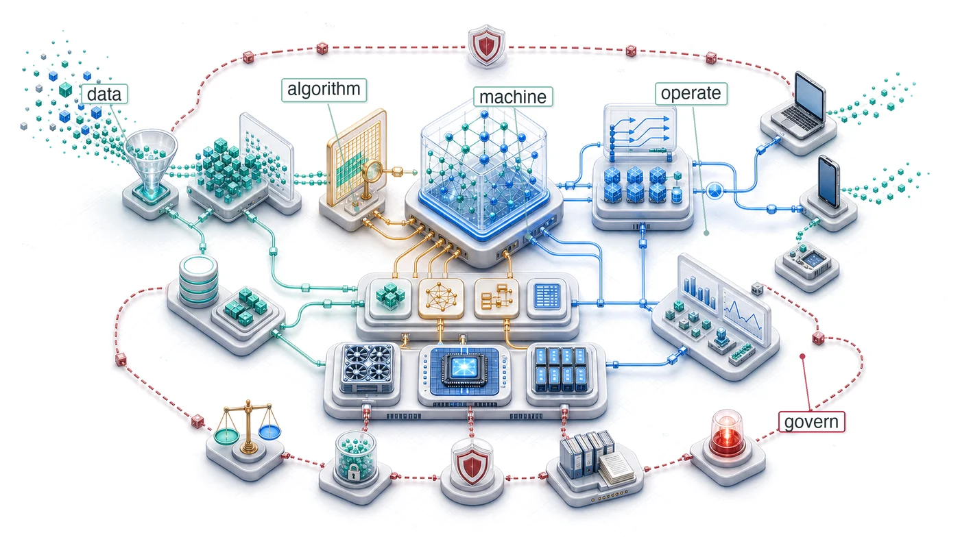
Purpose
What does mastering the full stack enable that expertise in any single layer cannot?
A single production decision can travel through the entire stack. A data pipeline decides which events count as training signal; that signal shapes the architecture that can learn the task; the architecture determines memory footprint and arithmetic intensity; those properties constrain hardware choice, quantization strategy, serving latency, drift monitoring, and governance obligations. Mastered individually, each layer is a valuable skill. Mastered together, they provide the ability to reason across boundaries. An engineer who understands only compression can shrink a model, but cannot predict whether the accuracy loss matters for the deployment context. An engineer who understands only serving can optimize latency, but cannot trace a performance regression to a data pipeline change three stages upstream. The discipline of ML systems engineering is the discipline of seeing these connections, where one team’s optimization becomes another team’s constraint. The principles governing these interactions, including constraint propagation, the memory wall, the training-serving inversion, dispatch overhead, communication cost, and the recurring cost of operating models in production, are not tied to any specific framework, hardware generation, or model family. Technologies will change, but the underlying physical constraints and trade-offs will endure. In D·A·M terms, what endures is the ability to look at a system that does not yet exist and reason about how its data, algorithm, and machine constraints will interact, where its bottlenecks will emerge, and which design decisions will prove irreversible. That D·A·M habit of thinking in systems rather than components is what separates an engineer who can build a part from one who can build the whole.
Learning Objectives
- Synthesize core ML systems principles into a framework for reasoning across Data, Algorithm, and Machine constraints
- Trace how data, architecture, compression, hardware, serving, operations, and governance decisions propagate constraints across an ML system
- Apply lighthouse-model reasoning to diagnose bottlenecks across cloud, mobile, edge, recommendation, and TinyML deployments
- Evaluate deployment trade-offs using latency budgets, memory movement, drift, responsibility, and sustainability constraints
- Design a systems engineering posture for emerging contexts before fleet-scale coordination costs dominate
Synthesizing ML Systems
Imagine deploying a new image classification model to a fleet of mobile devices. The architecture team chose depthwise separable convolutions for efficiency. The compression team quantized to INT8 for speed. The serving team hit a p99 latency target of 50 ms. Each team succeeded by its own metric, yet within weeks, user complaints arrive: accuracy has dropped by four percentage points on specific firmware and device cohorts. The cause is a subtle interaction between the quantization scheme and a firmware-specific image preprocessing path. No component is broken in isolation, but the data pipeline, architecture, compression strategy, hardware target, and monitoring infrastructure have coupled in production.
Responsible engineering is not an external layer added after optimization, but the discipline of specifying, testing, monitoring, and governing the whole system. That lesson now generalizes across this foundational material. ML systems are a different engineering problem from traditional software because the model is inseparable from the system that produces, serves, and monitors it.
The book began with the iron law of ML systems (principle 3). Its three terms—data movement, compute, and overhead—which once seemed abstract, now serve as primary engineering levers for quantitative analysis of systems that once seemed opaque. Building intelligence requires both algorithms and adherence to the silicon contract (principle 4), the physical and economic agreement between the model and the machine. Arithmetic intensity and roofline reasoning convert vague performance intuitions into quantitative engineering decisions (Williams et al. 2009).
The quantitative foundation leads to a broader point: contemporary artificial intelligence achievements are an emergent property of D·A·M co-design, not any single algorithmic insight. Machine learning belongs to the same engineering tradition that built reliable computers, where emergent capabilities arise from coordinating many parts together. The transformer architecture introduced an attention-based model family (Vaswani et al. 2017), and later large language model systems such as GPT-3 and Llama 2 show how that family scaled into a central workload for modern ML systems (Brown et al. 2020; Touvron et al. 2023). Its mathematical design alone does not explain its practical utility. That utility depends on integrating attention mechanisms with distributed training infrastructure, memory-efficient optimization techniques, and reliable operational frameworks.
Integration has concrete consequences. We often speak of the “model” as the weights file, a 500 MB blob of floating-point numbers. In a production environment, however, the weights are only one component of the true model, and often not the most important one. A model that produces perfect predictions is useless if it receives corrupted inputs, and a model that trains flawlessly will fail if it cannot be deployed reliably. The true model is the sum of the data pipeline that defines what the model sees, the training infrastructure that determines what it learns, the serving system that decides how it interacts with the world, and the monitoring loop that keeps it tethered to reality. Optimize the system, and the model improves. Neglect the system, and the model degrades. Systems engineering is not a wrapper around ML; it is the implementation of ML. The system is the model.
Checkpoint 1.1: Systems thinking
The system’s dependencies, feedback loops, and request path make its boundaries testable.
The integration
The holism
Tracing a request end to end, as the checkpoint asks, makes the same point structurally: system boundaries define model capabilities. That insight has guided the exploration throughout this book. The arc began by making the substrate explicit: data engineering (Data Engineering) and data selection (Data Selection) determined what the system could learn, neural computation (Neural Computation) and network architectures (Network Architectures) determined how that signal became computation, and training systems (Model Training) and frameworks (ML Frameworks) turned the computation into an executable optimization process.
Once the substrate existed, the engineering problem shifted from building to renegotiating constraints. Model compression (Model Compression) changed the accuracy-memory-latency trade-off; hardware acceleration (Hardware Acceleration) tested whether the resulting computation could actually feed the silicon; benchmarking (Benchmarking) supplied the measurement discipline needed to distinguish real speedup from artifact. Production then exposed the assumptions that survived the lab but failed under load: serving systems (Model Serving) had to meet latency budgets, operational practices (ML Operations) had to keep models healthy as distributions shifted, and responsible engineering (Responsible Engineering) had to evaluate whom the system served and where aggregate performance concealed subgroup failure. These chapters fill out the introduction’s five-pillar framework: data engineering, training systems, deployment infrastructure, operations and monitoring, and the ethics-and-governance pillar that threads Part IV rather than standing apart from it.
Each chapter contributed a piece. The real lesson, however, lies not in any individual piece but in how the pieces constrain each other. An architecture choice enabled a compression choice, which enabled an acceleration choice, which shaped a serving constraint, which defined an operational requirement. MobileNetV2’s depthwise-separable design targeted efficient mobile vision inference (Sandler et al. 2018), while integer-arithmetic quantization made INT8 deployment a practical inference path (Jacob et al. 2018). That combination can enable mobile NPU deployment, shape a p99 latency constraint, and require drift monitoring across heterogeneous device populations. Every decision propagated forward, and the engineer who understands only one layer cannot predict how changes ripple through the rest.

Architecture choices cascade into compression, serving, drift, and governance.
The lighthouse models provide a constraint map for reasoning about ML systems as wholes rather than as collections of parts. They trace the same interactions across chapters before the synthesis formalizes thirteen quantitative principles, including exact bounds and assumption-dependent diagnostic models, for reasoning about ML system behavior. Those principles then carry into three application domains, future directions where systems thinking will matter most, and the engineering responsibility that accompanies building systems of this power.
Lighthouse models: Constraint propagation
The five lighthouse models introduced in Iron Law of ML Systems made this constraint propagation concrete, serving as systems detectives throughout the book. Each revealed how different workloads expose different bottlenecks.
The five lighthouse workloads expose distinct constraint regimes:
- ResNet-50: Batch size can turn image inference from a memory-bound path into compute-bound throughput.
- GPT-2/Llama: Low-batch autoregressive decode is often bandwidth bound because each step reuses weights too little; batching, prefill, architecture, parallelism, and hardware can shift the bottleneck.
- MobileNetV2: Depthwise separable convolutions and INT8 quantization trade representational capacity for mobile NPU deployment in a power-constrained regime.
- DLRM: Terabyte-scale embedding tables can make memory capacity a binding constraint alongside memory bandwidth, forcing engineers to design around where data physically resides and how sparse operations behave.
- Keyword spotting (KWS)/Wake Vision: Sub-megabyte microcontroller models with always-on inference under milliwatt power budgets make every byte and milliwatt matter.
Together, these five workloads span the deployment spectrum from data center to microcontroller, probing the bottlenecks these principles diagnose and testing the optimization strategies developed throughout the book. The systems thinking we developed by tracing these lighthouses across chapters, from architecture design through training, optimization, and deployment, is the integrated perspective that distinguishes ML systems engineering from isolated algorithm development.
Table 1 traces this journey for a single model, MobileNetV2, showing how principles from across the book converge on one engineering artifact. The table walks through seven phases (from foundational constraints through architecture, training, compression, acceleration, serving, and operations) showing how each phase’s decisions propagate forward to shape what becomes possible in subsequent phases.
| Journey Phase | System Lens | MobileNetV2 Implementation |
|---|---|---|
| Foundations (Introduction) | The AI Triad | Bounded by machine constraints (Battery/Thermal) |
| Architecture (Network Architectures) | Algorithmic Efficiency | Depthwise Separable Convolutions: 8.7× fewer FLOPs for a representative 3-by-3, 256-output-channel layer and 13.7× fewer operations than ResNet-50 at ImageNet scale |
| Training (Model Training) | Throughput vs. Latency | Optimized for single-request mobile latency; data augmentation can improve robustness |
| Compression (Model Compression) | Navigating the Pareto Frontier | INT8 Quantization: FP32 uses 4× and FP16 uses 2× the per-value storage of INT8, with accuracy revalidated per deployment |
| Acceleration (Hardware Acceleration) | Honoring the Silicon Contract | Mapping kernels to Mobile NPUs (for example, Apple Neural Engine) to maximize hardware utilization |
| Serving (Model Serving) | Respecting the Latency Budget | \(\text{p99} < 50\) ms constraint; optimizing preprocessing (resize/normalize) to avoid CPU bottlenecks |
| Operations (ML Operations) | Managing System Entropy | Drift Monitoring: Detecting distribution shifts and tracking cohort-level accuracy across heterogeneous device populations and lighting conditions |
The table shows how decisions in one row constrain the options in the next. Architecture choices (depthwise separable convolutions) enabled compression choices (INT8 quantization), which in turn enabled acceleration choices (mobile NPU deployment). Constraint propagation recurs across ML systems, and the MobileNetV2 journey is one instance of that structure. The question is which quantitative tools recur across specific models and technologies. The answer lies in thirteen quantitative principles, some exact bounds and others assumption-dependent diagnostics.
Self-Check: Question
A production image classifier deployed across a mobile device fleet shows a 4-percentage-point drop in accuracy on specific handset cohorts. The weights file is unchanged, the compression team verified INT8 kernel speedups, and the serving team confirmed a P99 latency of 48 ms (under the 50 ms SLO). Which diagnostic posture is most consistent with the ‘system is the model’ thesis?
- Focus the investigation exclusively on serving execution, because runtime inference is the only stage operating during production.
- Trace the interaction between INT8 quantization scaling factors and firmware-specific image preprocessing paths, because production behavior is defined by the weights combined with the data pipeline, runtime hardware, and monitoring loop.
- Escalate to the architecture team to train wider convolutional layers, because an unchanged weights file implies that any remaining error must stem from model capacity.
- Treat the 4-point regression as acceptable random noise, because all engineering teams independently satisfied their local component metrics and the aggregate P99 latency is within budget.
A production recommender workload is dominated by terabyte-scale embedding tables where engineers spend significant effort deciding where data physically resides across storage tiers rather than optimizing dense matrix math. Which Lighthouse model embodies this constraint regime, and how does its primary bottleneck differ from low-batch GPT-2/Llama decoding?
- MobileNetV2; it is capacity-bound on microcontrollers, whereas autoregressive decoding is latency-bound by network packet round-trip times.
- ResNet-50; it is capacity-bound by image batch activation footprints in host DRAM, whereas LLM decode is compute-bound.
- Keyword Spotting (KWS); it is capacity-bound by microcontroller flash storage, whereas LLM decode is strictly compute-bound by tensor core peak FLOP/s.
- DLRM; it is capacity-bound by terabyte-scale embedding tables requiring physical data placement design, whereas low-batch LLM decode is memory-bandwidth-bound due to streaming weights with minimal arithmetic reuse per token.
Order the following phases of the MobileNetV2 Lighthouse Journey in their chronological lifecycle order as constraints propagate from initial requirements through deployment operations:
- Compression (INT8 quantization navigating the Pareto frontier)
- Acceleration (Mapping operators to mobile NPUs under the Silicon Contract)
- Foundations (Establishing battery, thermal, and machine constraints)
- Architecture (Depthwise separable convolutions reducing FLOPs)
- Operations (Cohort-level drift monitoring across heterogeneous devices)
- Serving (Enforcing P99 latency budgets under 50 ms)
True or False: If every engineering team in an ML organization independently satisfies its isolated component metric (e.g., architecture achieves an \(8.7\times\) FLOP reduction, compression achieves \(4\times\) weight reduction, and serving meets its P99 latency SLO), the integrated system is mathematically guaranteed to meet its end-to-end accuracy and correctness requirements in production.
The conclusion argues that ‘the system is the model.’ Explain why treating the model solely as a static weights file (e.g., a 500 MB floating-point binary) fails in production, and define what constitutes the ‘true model.’
Thirteen Quantitative Principles
Throughout this book, each part introduced quantitative tools for reasoning about ML system behavior. These thirteen quantitative principles deliberately mix exact mathematical bounds with engineering decompositions, fitted local models, policy requirements, and design heuristics. Table 2 collects all thirteen in one place, organized by the four parts that revealed them. Their value comes from applying each within its stated assumptions, not from treating every row as a universal law.
| # | Principle | Part | Core Equation/Statement | What It Predicts |
|---|---|---|---|---|
| 1 | Data-as-Code Principle | I: Foundations | Behavior \(=f\)(data, algorithm, code, randomness) | Data changes behavior; other inputs also matter |
| 2 | Data-Gravity Principle | I: Foundations | Move compute toward data when repeated transfer costs exceed placement costs | Depends on volume, reuse, network, and compute mobility |
| 3 | Iron Law of ML Systems | II: Build | \(T_{\text{seq}}=D_{\text{vol}}/\text{BW}+O/(R_{\text{peak}}\eta_{\text{hw}})+L_{\text{lat}}\); overlap ranges from max to sum | Stages may add or overlap |
| 4 | Silicon Contract | II: Build | \(I_{\text{ridge}}=R_{\text{peak}}/\text{BW}\); compare \(I_{\text{model}}\) with \(I_{\text{ridge}}\) | Diagnoses bandwidth- versus compute-limited operation |
| 5 | Pareto Frontier | III: Optimize | \(\nexists c'\ne c:\,[\forall k\,M_k(c')\ge M_k(c)]\land[\exists j\,M_j(c')>M_j(c)]\) | No distinct configuration dominates a frontier point |
| 6 | Arithmetic Intensity Law | III: Optimize | \(R_{\text{attain}} \le \min(R_{\text{peak}},\; I \times \text{BW})\) | More compute cannot raise a bandwidth ceiling |
| 7 | Energy-Movement Invariant | III: Optimize | \(E_{\text{total}}=\sum_j N_jE_j\); DRAM/FLOP cost ratio: 173–582× | Total energy depends on event counts and costs |
| 8 | Amdahl’s Law | III: Optimize | \(\text{Speedup} = \frac{1}{(1-f_{\text{parallel}}) + \frac{f_{\text{parallel}}}{S_{\text{parallel}}}}\) | The serial fraction caps all parallelism gains |
| 9 | Verification Gap | IV: Deploy | \(\Pr_{(X,Y)\sim P_{\text{deploy}}}[d(f(X),Y)\le\tau]\ge1-\epsilon\) | Specify distance, tolerance, population, and confidence |
| 10 | Statistical Drift Diagnostic | IV: Deploy | \(\text{Accuracy}(t)\approx\text{Accuracy}_0-\lambda\mathcal{D}(P_t\Vert P_0)\) | A local fit; drift need not lower quality |
| 11 | Training-Serving Skew Diagnostic | IV: Deploy | \(S_{\text{skew}}=\mathbb{E}_{X\sim P_{\text{deploy}}}[d(f_{\text{serve}}(X),f_{\text{train}}(X))]\) | Output mismatch signals risk, not accuracy loss |
| 12 | Latency Budget Principle | IV: Deploy | \(T_q\le L_{\text{budget}}\) | The product SLO selects \(q\) and its budget |
| 13 | Bias Feedback Model | IV: Deploy | \(\Delta_g(k)\approx\Delta_g(0)\alpha_{\text{fb}}^k\) with fitted \(\alpha_{\text{fb}}\) | Feedback may amplify harm; measure and intervene |
The thirteen principles are not independent axioms. They form an integrated framework connected by a single meta-principle: the conservation-of-complexity heuristic.1 Complexity removed from one interface often reappears in another part of the system, but this is not a physical conservation law and does not imply that every simplification has an equal compensating cost. Its value is diagnostic: after simplifying one component, check where validation, state, coordination, or operational burden changed. The test is whether the principles explain the same lighthouse bottlenecks from data, model, hardware, and deployment perspectives without contradicting one another.
1 Conservation-of-complexity heuristic: Tesler’s Law, a design aphorism, says that an application’s irreducible complexity must be handled somewhere in the interaction among user, application, and platform (Tesler 1984); extending it to all ML-system complexity is an analogy, not a physical law. Quantization may add validation burden, and abstraction may move implementation detail behind an interface, but good design can also remove accidental complexity outright. Large language model application pipelines illustrate a possible shift: simplifying the user-facing interface with shorter or vaguer prompts may move work into system prompts, retrieval, or output verification. Use the heuristic to search for displaced costs, not to assume that an equal compensating cost must exist.
Foundations: Where complexity originates (principles 1–2)
The data-as-code principle (1) and the data-gravity heuristic (principle 2), established in Part I and developed in Data Engineering, establish data as a major logical input and potential physical anchor. Behavior also depends on algorithm and implementation, while compute-to-data placement depends on volume, reuse, network cost, and compute mobility. Model behavior and architecture therefore inherit constraints from the data substrate.
The lighthouse models illustrate both principles directly. ResNet-50 and GPT-2 depend on both their architectures and their training data. DLRM’s terabyte-scale embedding tables can make a strong case for designing the system around where the data physically resides. These principles help explain why the compute-to-data pattern recurs across deployment contexts without turning it into a universal placement rule.
Build: How complexity becomes computation (principles 3–4)
The iron law (principle 3) and the silicon contract (principle 4) guide decisions in constructing an ML system. The iron law’s three-term decomposition (introduced in Iron Law of ML Systems) identifies which lever to pull; the silicon contract determines which term dominates for a given architecture-hardware pair. As the lighthouse journey showed, each model can expose a different constraint regime: batched ResNet-50 inference can be compute bound, low-batch Llama decode can be bandwidth bound, DLRM can be capacity bound, and MobileNetV2 reshapes its computation to fit mobile NPU constraints. Bottleneck diagnostic maps each of these regimes to the optimizations that pay off and the ones that waste effort, turning the diagnosis of compute-bound versus bandwidth-bound versus capacity-bound into an action plan. Model Training confirmed that training time falls most when engineers optimize the dominant term rather than distributing effort uniformly.
Optimize: How constraints shape trade-offs (principles 5–8)
The four optimization principles form a tightly coupled diagnostic chain. The Pareto frontier (principle 5) identifies nondominated trade-offs after objective directions are normalized: quantization trades precision for memory traffic, pruning trades capacity for speed, and distillation trades training compute for inference efficiency. The arithmetic intensity law (principle 6) diagnoses whether compute or bandwidth sets the ideal ceiling. The energy-movement invariant (principle 7) combines per-event costs with event counts: in the book’s reference constants, one DRAM access costs about 173–582× as much as one FP32/FP16 arithmetic operation, but workload-total dominance depends on how many of each occur. Amdahl’s Law (principle 8) sets the ceiling on any parallelism gain, explaining why data loading and preprocessing can become bottlenecks in highly optimized systems.
MobileNetV2 (our lighthouse from Network Architectures) navigates all four simultaneously: depthwise separable convolutions reshape the Pareto frontier (Sandler et al. 2018), INT8 quantization exploits the arithmetic intensity law by increasing operations per byte through reduced memory traffic (Jacob et al. 2018), and the resulting energy savings respect the energy-movement invariant while Amdahl’s Law explains why a preprocessing stage that remains unaccelerated can limit end-to-end speedup. The KWS lighthouse pushes these trade-offs to their extreme, where sub-megabyte models on microcontrollers leave zero margin for waste on any axis.
Deploy: How reality defeats assumptions (principles 9–13)
The deployment principles address failures that bench testing cannot rule out: a system can work correctly on the bench yet fail silently in production. The verification gap (principle 9) means statistical verification holds only over a stated deployment population, task distance, tolerance, target error, and finite-sample confidence procedure; testing estimates behavior rather than proving correctness for every future input. The statistical drift diagnostic (principle 10) detects distribution change but does not determine whether accuracy worsens, stays constant, or improves, so a local degradation curve is valid only when fitted against outcomes. The training-serving skew diagnostic (principle 11) is likewise a risk indicator rather than a universal accuracy-loss equation, although preprocessing or numerical differences can still cause quality changes. The latency budget (principle 12) constrains serving at the quantile selected by the product requirement, which may be p95, p99, or another tail measure. Finally, the bias feedback model (principle 13) can represent disparity amplification, but an exponential recurrence requires a measured, approximately constant feedback factor and no effective intervention.
The five deployment principles explain why ML Operations devoted extensive attention to monitoring, drift detection, feature stores, and disaggregated subgroup metrics: operational infrastructure must surface silent failures and connect evidence to response. A DLRM recommendation system that achieves excellent offline accuracy still needs parity checks when training-serving skew corrupts feature values (principle 11) and outcome checks when user behavior drifts seasonally (principle 10). GPT-2/Llama serving must respect its selected latency quantile through techniques such as continuous batching and speculative decoding, as detailed in Model Serving, because excessive response time may violate the product requirement. A loan approval system can satisfy every other principle while still systematically denying credit to underserved communities, and feedback can compound the harm unless disaggregated subgroup monitoring detects it and triggers review.
The integrated framework
The thirteen principles are not a checklist to apply sequentially. They form a web of mutual constraints. The conservation-of-complexity heuristic prompts engineers to look for where a local simplification changes burdens elsewhere.
We can trace these mutual constraints concretely by following what happens when an engineer quantizes a model from FP16 to INT8. This single decision navigates the Pareto frontier (principle 5), trading precision for memory traffic. The consequences do not stop there: quantization changes the model’s silicon contract (principle 4), shifting where it sits on the arithmetic intensity curve (principle 6) and altering its energy profile (principle 7). When that quantized model is deployed, the latency budget (principle 12) governs whether the speedup meets the service-level objective (SLO), while deployment validation must verify that the quantized serving path preserves the behavior accepted during compression testing. A single quantization decision ripples through the Pareto frontier, silicon contract, and latency budget simultaneously, where a win in one (memory traffic) must be validated against a risk in another (numerical error).
That trace does not require every principle to apply at once. It shows how the relevant principles become active as a decision moves from model representation to hardware execution to production validation. Data placement affects where the model can run, Amdahl’s Law limits how much the faster kernel can improve the whole request path, verification bounds the resulting accuracy loss, and outcome monitoring tests whether the validated behavior persists after deployment. The engineer’s task is to trace displaced costs rather than assume that complexity is conserved.
A small deployment proposal makes this web of constraints concrete.
Checkpoint 1.2: Applying the principles
A colleague proposes quantizing your model from FP32 to INT8 to reduce serving costs.
Trace the principles
To see this cycle of mutual constraint in action, trace the flow in figure 1. The four phases (Foundations, Build, Optimize, Deploy) surround a central hub representing the conservation-of-complexity heuristic, and the arrows map the flow of engineering decisions: each phase’s choices constrain what becomes possible in the next, and the cycle eventually feeds back to the beginning. Decisions in Build constrain Optimize, while production evidence such as drift, skew, and outcome changes can feed back into Foundations. The engineer’s role is to manage this flow, ensuring that displaced burdens land where they can be handled efficiently.
The Deploy-to-Foundations feedback arrow is central to this cycle. Principles nine through thirteen expose signals and constraints that may require a corrected release, fallback, new data, retraining, or a fresh optimization pass. When one appears, engineers must diagnose which response fits the cause rather than react automatically to a drift alarm. The cycle operates within the single-system scope of this book: the goal is not to name every future architecture, but to make feedback visible early enough that engineers can redesign before failures compound.
\begin{tikzpicture}[line join=round,font=\sffamily]

\tikzset{
Box/.style={align=flush center,
    inner sep=4pt,
    node distance=1.4,
    draw=OrangeLine,
    line width=0.75pt,
    rounded corners,
    fill=OrangeL!30,
    text width=25mm,
    minimum width=25mm, minimum height=10mm
  },
Box2/.style={Box, draw=VioletLine, fill=VioletL2!70,align=left,
    text width=36mm, minimum width=36mm, minimum height=10mm
  },
  }

\tikzset{%
planet/.style = {circle, draw=yellow!50!red!90,semithick, fill=yellow!30,line width=1.5pt,
                    font=\sffamily\bfseries,
                    minimum size=24mm, inner sep=1mm,align=flush center},
satellite/.style = {circle, draw=none, semithick, fill=#1!10,
                    text width=26mm, inner sep=1pt, align=flush center,minimum size=20mm,minimum height=12mm},
TxtC/.style = {font=\small\sffamily,text width=44mm,align=flush center},
arr/.style = {-{Triangle[length=3mm,width=6mm]}, color=#1!60,
                    line width=3mm, shorten <=1mm, shorten >=1mm},
LineA/.style = {violet!60,{Circle[line width=1.5pt,fill=white,length=7.5pt]}-,line width=2.0pt,shorten <=-4pt},
LineAA/.style={violet!30,dashed, line width=1.0pt,{-{Triangle[width=1.0*6pt,length=1.6*6pt]}},shorten <=3pt,shorten >=2pt}
}

\tikzset{pics/brain/.style = {
        code = {
        \pgfkeys{/channel/.cd, #1}
\begin{scope}[local bounding box=BRAIN,scale=\scalefac, every node/.append style={transform shape}]
\draw[fill=\filllcolor,line width=\Linewidth](-0.3,-0.10)to(0.08,0.60)
to[out=60,in=50,distance=3](-0.1,0.69)to[out=160,in=80](-0.26,0.59)to[out=170,in=90](-0.46,0.42)
to[out=170,in=110](-0.54,0.25)to[out=210,in=150](-0.54,0.04)
to[out=240,in=130](-0.52,-0.1)to[out=300,in=240]cycle;
\draw[fill=\filllcolor,line width=\Linewidth]
(-0.04,0.64)to[out=120,in=0](-0.1,0.69)(-0.19,0.52)to[out=120,in=330](-0.26,0.59)
(-0.4,0.33)to[out=150,in=280](-0.46,0.42)
%
(-0.44,-0.03)to[bend left=30](-0.34,-0.04)
(-0.33,0.08)to[bend left=40](-0.37,0.2) (-0.37,0.12)to[bend left=40](-0.45,0.14)
(-0.26,0.2)to[bend left=30](-0.24,0.13)
(-0.16,0.32)to[bend right=30](-0.27,0.3)to[bend right=30](-0.29,0.38)
(-0.13,0.49)to[bend left=30](-0.04,0.51);
\draw[rounded corners=0.8pt,line width=1.5*\Linewidth,\drawcircle,-{Circle[fill=\filllcolor,length=4.15pt]}](-0.23,0.03)--(-0.15,-0.03)--(-0.19,-0.18)--(-0.04,-0.28);
\draw[rounded corners=0.8pt,line width=1.5*\Linewidth,\drawcircle,-{Circle[fill=\filllcolor,length=4.15pt]}](-0.17,0.13)--(-0.04,0.05)--(-0.06,-0.06)--(0.14,-0.11);
\draw[rounded corners=0.8pt,line width=1.5*\Linewidth,\drawcircle,-{Circle[fill=\filllcolor,length=4.15pt]}](-0.12,0.23)--(0.31,0.0);
\draw[rounded corners=0.8pt,line width=1.5*\Linewidth,\drawcircle,-{Circle[fill=\filllcolor,length=4.15pt]}](-0.07,0.32)--(0.06,0.26)--(0.16,0.33)--(0.34,0.2);
\draw[rounded corners=0.8pt,line width=1.5*\Linewidth,\drawcircle,-{Circle[fill=\filllcolor,length=4.15pt]}](-0.01,0.43)--(0.06,0.39)--(0.18,0.51)--(0.31,0.4);
\end{scope}
     }
  }
}

%brick
\tikzset{
  cigla/.style={ inner sep=0pt,anchor=west,
    node distance=1.4pt,
    draw=none,
    line width=0.1pt,
    rounded corners=1pt,
    fill=\filllcolor,
    minimum width=4mm, minimum height=2mm
  },
    cigla1/.style={cigla,fill=\filllcirclecolor},
pics/brick/.style = {
        code = {
        \pgfkeys{/channel/.cd, #1}
\begin{scope}[shift={($(0,0)+(0,0)$)},scale=\scalefac,every node/.append style={transform shape}]
\path[clip] (-1.05,-0.52)rectangle (0.71,0.45);
\node[cigla](C1) at (-1.03,-0.4){};
\node[cigla1,right= of C1](C2){};
\node[cigla,right= of C2](C3){};
\node[cigla1,right= of C3](C4){};
%
\node[cigla,above right= of C1,anchor=south](C11){};
\node[cigla1,right= of C11](C12){};
\node[cigla,right= of C12](C13){};
\node[cigla1,right= of C13](C14){};
%
\node[cigla,above right= of C11,anchor=south](C21){};
\node[cigla1,right= of C21](C22){};
\node[cigla,right= of C22](C23){};
%
\node[cigla,above right= of C21,anchor=south](C31){};
\node[cigla1,right= of C31](C32){};
\node[cigla,right= of C32](C33){};
\end{scope}
    }
  }
}
%vaga
\tikzset{
pics/vaga/.style = {
        code = {
        \pgfkeys{/channel/.cd, #1}
\begin{scope}[shift={($(0,0)+(0,0)$)},scale=\scalefac,every node/.append style={transform shape}]
\node[rectangle,minimum width=2mm,minimum height=22mm,
draw=none, fill=\filllcolor,line width=\Linewidth](1R) at (0,-0.95){};
\fill[fill=\filllcolor!60!black](230:2.8)arc(230:310:2.8)--cycle;%circle(2.9);
%LT
\node [semicircle, shape border rotate=180,  anchor=chord center,
      minimum size=11mm, draw=none, fill=\filllcirclecolor](LT) at (-2,-0.5) {};
\node [circle,  minimum size=4mm, draw=none, fill=\filllcirclecolor](T1) at (-2,1.25) {};
\draw[draw=\drawcolor,line width=1.2*\Linewidth,shorten <=3pt,shorten >=3pt](T1)--(LT);
\draw[draw=\drawcolor,line width=1.2*\Linewidth,shorten <=3pt,shorten >=3pt](T1)--(LT.30);
\draw[draw=\drawcolor,line width=1.2*\Linewidth,shorten <=3pt,shorten >=3pt](T1)--(LT.150);
%DT
\node [semicircle, shape border rotate=180,  anchor=chord center,
      minimum size=11mm, draw=none, fill=\filllcirclecolor!70!black](DT) at (2,-0.5) {};
\node [circle,  minimum size=4mm, draw=none, fill=\filllcirclecolor!70!black](T2) at (2,1.25) {};
\draw[draw=\drawcolor,line width=1.2*\Linewidth,shorten <=3pt,shorten >=3pt](T2)--(DT);
\draw[draw=\drawcolor,line width=1.2*\Linewidth,shorten <=3pt,shorten >=3pt](T2)--(DT.30);
\draw[draw=\drawcolor,line width=1.2*\Linewidth,shorten <=3pt,shorten >=3pt](T2)--(DT.150);
%
\node[draw=none,rectangle,minimum width=32mm,minimum height=1.5mm,inner sep=0pt,
fill=\filllcolor!60!black]at(0,1.25){};
\node[draw=white,fill=\filllcolor,line width=2*\Linewidth,ellipse,minimum width=9mm,  minimum height=15mm](EL)at(0,0.85){};
\node[draw=white,fill=\filllcolor!60!black,line width=2*\Linewidth,circle,minimum size=10mm](2C)at(0,2.05){};
\end{scope}
    }
  }
}
%llm
\tikzset{
pics/llm/.style = {
        code = {
        \pgfkeys{/channel/.cd, #1}
\begin{scope}[shift={($(0,0)+(0,0)$)},scale=\scalefac,every node/.append style={transform shape}]
\node[circle,minimum size=12mm,draw=\drawcolor, fill=\filllcolor!70,line width=0.5*\Linewidth](C\picname) at (0,0){};
\def\startangle{90}
\def\radius{1.15}
\def\radiusI{1.1}
\foreach \i [evaluate=\i as \j using \i+1] [count =\k] in {0,2,4,6,8} {
\pgfmathsetmacro{\angle}{\startangle - \i * (360/8)}
\draw[draw=black,-{Circle[black ,fill=\filllcirclecolor,length=5.5pt,line width=0.5*\Linewidth]},line width=1.5*\Linewidth](C\picname)--++(\startangle - \i*45:\radius) ;
\node[circle,draw=black,fill=\filllcirclecolor!80!red!50,inner sep=3pt,line width=0.5*\Linewidth](2C\k)at(\startangle - \j*45:\radiusI) {};
}
\draw[line width=1.5*\Linewidth](2C1)--++(-0.5,0)|-(2C2);
\draw[line width=1.5*\Linewidth](2C3)--++(0.5,0)|-(2C4);
\node[circle,minimum size=12mm,draw=\drawcolor, fill=\filllcolor!70,line width=0.5*\Linewidth]at (0,0){};
\end{scope}
    }
  }
}
%battery
\tikzset{
pics/battery/.style = {
        code = {
        \pgfkeys{/channel/.cd, #1}
\begin{scope}[shift={($(0,0)+(0,0)$)},scale=\scalefac,every node/.append style={transform shape}]
\node[rectangle,minimum width=35mm,minimum height=8mm,draw=\drawcolor,
rounded corners=4pt,fill=\filllcirclecolor,line width=\Linewidth](2R\picname) at (1,0){};
\node[rectangle,minimum width=45mm,minimum height=22mm,draw=\drawcolor,
rounded corners=4pt,fill=\filllcolor,line width=\Linewidth](R\picname) at (0,0){};
\node[rectangle,minimum width=5mm,minimum height=18mm,draw=none,
fill=green,line width=\Linewidth](3R\picname) at ($(R\picname.west)!0.5!(R\picname.east)$){};
\node[rectangle,minimum width=5mm,minimum height=18mm,draw=none,
fill=green,line width=\Linewidth](3R\picname) at ($(R\picname.west)!0.33!(R\picname.east)$){};
\node[rectangle,minimum width=5mm,minimum height=18mm,draw=none,
fill=green,line width=\Linewidth](3R\picname) at ($(R\picname.west)!0.16!(R\picname.east)$){};

\end{scope}
    }
  }
}
%rocket
\tikzset{
pics/rocket/.style = {
        code = {
        \pgfkeys{/channel/.cd, #1}
\begin{scope}[shift={($(0,0)+(0,0)$)},scale=\scalefac,every node/.append style={transform shape},line cap = round]
%vrh
\draw[fill=\filllcolor,draw=\drawcolor,line width=\Linewidth](-0.26,0.5)to[bend right=12](0.26,0.5)to[bend right=7] (0,0.85)to[bend right=7] cycle;
%krila
\draw[fill=\filllcolor!70!red,draw=\drawcolor,line width=\Linewidth,rounded corners=1pt](-0.2,-0.7)--(-0.45,-0.9)--(-0.567,-0.4)--(-0.3,-0.17)--cycle;
\draw[fill=\filllcolor!70!red,draw=\drawcolor,line width=\Linewidth,rounded corners=1pt](0.2,-0.7)--(0.45,-0.9)--(0.567,-0.4)--(0.3,-0.17)--cycle;
%rep
\draw[fill=\filllcolor!70!green,draw=\drawcolor,line width=\Linewidth](0.16,-0.76)--(0.22,-0.9)--(-0.2,-0.9)--(-0.15,-0.76)--cycle;
%body
\draw[fill=\filllcolor,draw=\drawcolor,line width=\Linewidth](-0.2,-0.7)--(0.2,-0.7)to[out=75,in=320](0,0.85)to[out=220,in=105] cycle;
%krug
\node[circle,draw=\drawcolor,minimum size=4mm,fill=\filllcirclecolor,line width=\Linewidth]{};
\draw[draw=\drawcolor,line width=1.5*\Linewidth](0,-0.99)--(0,-1.3);
\draw[draw=\drawcolor,line width=1.5*\Linewidth](-0.11,-0.99)--(-0.11,-1.2);
\draw[draw=\drawcolor,line width=1.5*\Linewidth](0.11,-0.99)--(0.11,-1.2);
\end{scope}
    }
  }
}
\pgfkeys{
  /channel/.cd,
   Depth/.store in=\Depth,
  Height/.store in=\Height,
  Width/.store in=\Width,
  filllcirclecolor/.store in=\filllcirclecolor,
  filllcolor/.store in=\filllcolor,
  drawcolor/.store in=\drawcolor,
  drawcircle/.store in=\drawcircle,
  scalefac/.store in=\scalefac,
  Linewidth/.store in=\Linewidth,
  picname/.store in=\picname,
  filllcolor=BrownLine,
  filllcirclecolor=violet!20,
  drawcolor=black,
  drawcircle=violet,
  scalefac=1,
  Linewidth=0.5pt,
  Depth=1.3,
  Height=0.8,
  Width=1.1,
  picname=C
}

\def\radius{3.9}
\def\startangle{90}

\foreach \i/\j/\sho [count=\k from 0] in {
%green!79!black
white/{\textbf{}\\ }/15pt,
%magenta!60!
white/{\textbf{}\\ }/15pt,
%gray
white/{\textbf{}\\}/15pt,
%cyan
white/{\textbf{}\\ }/15pt
}
{
%Satelit
\pgfmathsetmacro{\angle}{\startangle - \k * (360/4)}
\node (s\k) [satellite=\i, font=\footnotesize\sffamily] at (\angle:\radius) {};
 \node[TxtC,below=0pt of s\k]{\j};
}
%logos
%brick
\pic[shift={(0.15,0.15)}] at  (s3) {brick={scalefac=1.1,picname=1,filllcolor=red!70!black!80,Linewidth=1.0pt,filllcirclecolor=red!90!black!50}};
%llm
\pic[shift={(0,0)}] at  (s0){llm={scalefac=0.9,drawcolor=BlueLine,filllcolor=BlueLine!10!, Linewidth=1.25pt,filllcirclecolor=red}};
%brain
\pic[shift={(0.1,-0.16)}] at  (s0){brain={scalefac=0.8,picname=1,filllcolor=orange!30!, filllcirclecolor=cyan!55!black!60, Linewidth=0.5pt}};
%battery
\pic[shift={(0,0)}] at  (s1){battery={scalefac=0.38,picname=1, drawcolor=BrownLine,filllcolor=BrownLine!10!, Linewidth=1.5pt,filllcirclecolor=BrownLine}};
%rocket
\pic[shift={(0,0.2)}] at  (s2){rocket={scalefac=1.1,picname=1, drawcolor=black,filllcolor=cyan!10!, Linewidth=1.0pt,filllcirclecolor=red}};
%center
\node[circle, draw=BrownLine, dashed,thick, fill=none,minimum size=26mm](CE)at(0,0){};
 \node[TxtC,below=0pt of CE]{Conservation\\ of Complexity};
 \pic[shift={(0,0)}] at  (0,0){vaga={scalefac=0.35,picname=1,filllcolor=BlueLine,  Linewidth=1.0pt,filllcirclecolor=orange}};
\def\ra{26mm}
\foreach \i [count=\k from 0] in{360,320,140,135}{
\pgfmathtruncatemacro{\newX}{\i + 90} %
\draw[line width=2.6pt,violet]
   (s\k)+(\i:0.5*\ra) arc[start angle=\i, end angle=\newX, radius=0.5*\ra];
}
 \draw[LineA](s0.35)--++(0:1)coordinate(MA);
 \node[Box,anchor=west](FO)at(MA){\textbf{Build}\\ (Model)};
 \draw[LineA](s1.355)--++(345:1)coordinate(ST);
 \node[Box,anchor=west](PR)at(ST){\textbf{Optimize}\\ (Hardware)};
 \draw[LineA](s2.185)--++(200:3.25)coordinate(DE);
 \node[Box,anchor=west](DEP)at(DE){\textbf{Deploy}\\(Operations)};
 \draw[LineA](s3.180)--++(180:3.9)coordinate(FO);
 \node[Box,anchor=west](FND)at(FO){\textbf{Foundations}\\(Data)};
%
\draw[-{Triangle[width=18pt,length=8pt]}, line width=10pt,cyan!40] (60:\radius)
arc[radius=\radius, start angle=60, end angle= 16];
\coordinate (AR1) at (38:\radius);
\draw[-{Triangle[width=18pt,length=8pt]}, line width=10pt,cyan!40] (340:\radius)
arc[radius=\radius, start angle=340, end angle= 290];
\coordinate (AR2) at (315:\radius);
\draw[-{Triangle[width=18pt,length=8pt]}, line width=10pt,cyan!40] (240:\radius)
arc[radius=\radius, start angle=240, end angle= 200];
\coordinate (AR3) at (225:\radius);
\draw[-{Triangle[width=18pt,length=8pt]}, line width=10pt,cyan!40] (160:\radius)
arc[radius=\radius, start angle=160, end angle= 114];
\coordinate (AR4) at (137:\radius);
%
 \draw[LineA](AR1)--++(0:1.3)coordinate(MA);
 \node[Box2,anchor=west]at(MA){3. Iron Law\\
4. Silicon Contract};
 \draw[LineA](AR2)--++(340:1.6)coordinate(MA1);
 \node[Box2,anchor=west]at(MA1){5. Pareto Frontier\\
6. Arith. Intensity\\
7. Energy-Movement\\
8. Amdahl’s Law};
 \draw[LineA](AR3)--++(180:6.5)coordinate(MA2);
 \node[Box2,anchor=west]at(MA2){9. Verification Gap\\
10. Stat. Drift\\
11. Skew Diagnostic\\
12. Latency Budget\\
13. Bias Feedback};
 \draw[LineA](AR4)--++(180:6.5)coordinate(MA3);
 \node[Box2,anchor=west]at(MA3){1. Data as Code\\
2. Data Gravity};
\end{tikzpicture}Tracing a quantization proposal through four principles is one diagnostic pass; the same habit applies when the bottleneck is not an optimization proposal but the cost of serving a single generated token.
Napkin Math 1.1: The cost of a token
Physics:
- Model-weight byte volume moved \((D_{\text{vol}})\): 70 billion parameters \(\times\) 2 bytes (FP16) =
- Compute \((O)\): \(O \approx 2 \times P =\) 140 GFLOP per token, where \(P\) is the parameter count.
- Hardware: Two H100s with aggregate \(\text{BW}\) = 6.70 TB/s, \(R_{\text{peak}} \approx\) 1978 TFLOP/s FP16.
Math:
- Time to move data: \(T_{\text{mem}} = \frac{140 \text{ GB}}{6700 \text{ GB/s}} \approx 20.9 \text{ ms}\)
- Time to compute: \(T_{\text{comp}} = \frac{140 \times 10^9 \text{ FLOP}}{1978 \times 10^{12} \text{ FLOP/s}} \approx 0.07 \text{ ms}\)
Systems insight:
The idealized memory-transfer lower bound \(T_{\text{mem}}\) is 295.2× larger than the peak-compute lower bound \(T_{\text{comp}}\). Under this batch-one model, decode is heavily bandwidth bound (arithmetic intensity \(\approx 1\) FLOP/byte). Batching can increase reuse, while quantization can reduce weight traffic. Optimizing only compute execution can reduce realized compute time toward the 0.07 ms lower bound, but it cannot reduce the 20.9 ms memory-transfer lower bound.
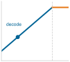
In this batch-one lower-bound model, decode sits left of the roofline ridge in the bandwidth-bound regime.
This calculation shows the framework operating as a diagnostic instrument rather than an abstract taxonomy. The chapters applied these bounds, models, and heuristics to specific engineering decisions, often without naming them explicitly. Tracing those applications across three domains—building foundations, engineering for scale, and navigating production reality—reveals how the framework has guided the analysis throughout the book.
Self-Check: Question
Consider serving one token at batch size 1 from a 70-billion-parameter Llama 2 model in FP16 (\(D_{\text{vol}} = 140\text{ GB}\), \(O \approx 140\text{ GFLOP}\)) sharded across two NVIDIA H100 GPUs (aggregate \(\text{BW} = 6.70\text{ TB/s}\), aggregate \(R_{\text{peak}} = 1,978\text{ TFLOP/s}\)). What are the idealized lower bounds for memory transfer (\(T_{\text{mem}}\)) and peak compute (\(T_{\text{comp}}\)), and what systems optimization strategy does this diagnostic dictate?
- Memory transfer time \(T_{\text{mem}} \approx 0.07\text{ ms}\) and compute time \(T_{\text{comp}} \approx 20.9\text{ ms}\); because compute time dominates by \(295\times\), the engineering team should prioritize hand-tuning tensor core matrix multiplication kernels.
- Memory transfer time \(T_{\text{mem}} \approx 2.09\text{ ms}\) and compute time \(T_{\text{comp}} \approx 2.09\text{ ms}\); because the workload operates exactly at the roofline ridge point, compute optimizations and memory optimizations provide identical returns.
- Memory transfer time \(T_{\text{mem}} \approx 20.9\text{ ms}\) and compute time \(T_{\text{comp}} \approx 0.07\text{ ms}\); because the memory bound is \(\approx 295\times\) larger than the compute bound, decode is heavily bandwidth-bound, meaning kernel FLOP tuning yields negligible speedup while batching and quantization directly reduce latency.
- Memory transfer time \(T_{\text{mem}} \approx 41.8\text{ ms}\) and compute time \(T_{\text{comp}} \approx 0.14\text{ ms}\); because sharding across two GPUs doubles the communication overhead, execution time increases by \(2\times\) relative to a single GPU.
According to the Energy-Movement Invariant (\(E_{\text{total}} = \sum_j N_j E_j\)), accessing off-chip DRAM requires approximately 100 to 1,000 times more energy than executing a single FP16 or FP32 arithmetic operation. What is the direct systems design implication of this physical reality?
- Inference engines should prioritize minimizing total ALU operations above all else, even if intermediate tensors must be repeatedly written to and read from off-chip DRAM.
- Hardware accelerators consume identical energy regardless of whether memory accesses hit on-chip SRAM or off-chip DRAM, because memory controller power is fixed.
- Quantization saves energy exclusively by simplifying ALU multiplication logic, while memory traffic volume has negligible impact on total package power.
- Architectures and runtimes must maximize on-chip data reuse (e.g., via operator kernel fusion, SRAM tiling, and weight quantization), because eliminating off-chip DRAM round-trips yields orders-of-magnitude greater energy savings than reducing arithmetic FLOPs.
True or False: The conservation-of-complexity heuristic is an exact physical conservation law of computer science that proves every simplification in an ML pipeline interface creates an identical, mathematically equal compensating burden in another component.
The thirteen quantitative principles are unified by a central meta-heuristic known as the ____ heuristic, which reminds engineers that simplifying one interface often displaces validation, state, or operational burdens to another part of the system.
In the Cycle of ML Systems diagram (figure 1), the Deploy phase contains an explicit feedback arrow returning to Foundations (Data). Explain what production signals activate this feedback loop and why automated rollback is insufficient when the cause is external statistical drift.
Principles in Practice
A team that memorizes all thirteen principles but cannot identify their assumptions or apply them to a real deployment decision has learned nothing. The test is the same across the three domains that span the ML lifecycle: building technical foundations, engineering for scale, and navigating production reality. Systems thinking connects what isolated component analysis cannot.
Building technical foundations
The data-as-code principle (1) shaped Data Engineering, echoing Karpathy’s Software 2.0 framing of datasets and model architecture as source code (Karpathy 2017) while recognizing that algorithms and serving code also affect behavior. Mathematical foundations (Neural Computation) established the computational patterns relevant to the silicon contract: the matrix multiplications at the heart of neural computation determine arithmetic intensity, whose position relative to the hardware ridge point helps diagnose whether a workload is bandwidth or compute limited. Framework selection (ML Frameworks) illustrated the silicon contract’s practical consequence: each framework constrains graph optimization, memory management, hardware backend support, and the deployment paths that remain open. An engineer who selects a framework without considering those implications may discover too late that the chosen path forecloses the most efficient deployment option.
Foundational choices (what data to curate, which computational primitives to rely on, which framework to adopt) propagate into later engineering decisions. That propagation becomes especially visible when a system must scale beyond a single machine, where the iron law’s three terms expand from chip-level quantities to cluster-level constraints.
Engineering for scale
Training systems (Model Training) demonstrated the iron law in action: data parallelism can reduce per-step compute time by distributing work across GPUs while adding communication, mixed precision can reduce data movement for tensors represented in FP16 rather than FP32, and gradient checkpointing trades recomputation for memory capacity, each technique pulling a different lever of the same three-term equation. Model compression (Model Compression) navigated the Pareto frontier directly: MobileNetV2’s INT8 quantization and DLRM’s embedding pruning each traded one metric for another, while the arithmetic intensity law diagnosed which trade-off would yield the greatest return for a given hardware target.
Building and optimizing a model, however, is only half the engineering challenge. The other half begins the moment the model leaves the training cluster and enters production, where statistical requirements, fitted diagnostics, and SLO policies govern behavior and where the optimizations that worked on the bench must survive the unpredictability of real-world traffic.
Navigating production reality
The transition from training to inference often changes optimization objectives: where training maximizes throughput over days, interactive inference may optimize a selected tail-latency quantile in milliseconds. The illustrative scenario uses a 50 ms mean and a 2,000 ms p99, so the selected tail is 40\(\times\) the mean; another product may specify p95, p99.9, or separate deadlines by request class. Tail-latency analysis shows why mean latency can hide the requests that dominate user experience (Dean and Barroso 2013). In ML serving, tail spikes can arise from garbage collection pauses in Python-based inference frameworks, dynamic batching that forms suboptimally under uneven traffic, or autoregressive generation in which a long prompt or output drives much more work than a typical short response.

Mean latency hides the tail; the selected tail quantile governs the SLO.
Beyond technical performance, Responsible Engineering broadened the framework to include societal impact. Verification requirements motivate monitoring for fairness violations alongside performance: tracking prediction distributions across demographic groups, detecting bias amplification over time (principle 13), and alerting on unexplained accuracy disparities. Drift monitoring also applies to subgroup distributions and outcomes, where accuracy may change for underrepresented populations even as aggregate metrics remain stable. Responsible AI is therefore an integral dimension of systems engineering, a first-class design constraint governed by the same measurement discipline as performance.
The three domains demonstrate that the thirteen principles are working tools rather than universal axioms. The question now is where their assumptions will be tested next, as ML systems expand into new deployment contexts, confront new failure modes, and pursue increasingly ambitious goals.
Self-Check: Question
A team chooses an ML framework primarily for its familiar Python syntax, only to discover months later that deploying the model to mobile NPUs and edge accelerators requires painful manual kernel rewrites because the framework lacks mature compiler lowering and graph optimization for those backends. Why does the Silicon Contract lens classify framework selection as an architectural commitment rather than an ergonomic preference?
- Frameworks embody fundamental architectural commitments to intermediate representations (IR), memory allocators, operator fusion passes, and backend compiler targets, which dictate whether the hardware’s peak efficiency can be realized downstream.
- Standard exchange formats such as ONNX are mathematically guaranteed to recover 100% of native hardware performance regardless of which framework was used during training.
- Frameworks operate exclusively as UI wrappers; hardware execution speed is determined solely by the neural network weights file.
- Modern hardware accelerators execute Python bytecode directly on silicon, so framework differences only affect model training time.
A production serving dashboard for an interactive conversational assistant reports an average (mean) latency of 50 ms. However, user satisfaction metrics are declining, and detailed telemetry reveals a P99 tail latency of 2,000 ms (a \(40\times\) gap over the mean), violating the product SLO (\(T_{0.99} \le 200\text{ ms}\)). Which systems mechanism is a primary root cause of this massive tail spike in ML inference?
- Uniform degradation of memory bus bandwidth across all simultaneous client connections.
- A 40x increase in model weight parameters triggered dynamically whenever traffic surges.
- Heavy-tailed sequence lengths in autoregressive decoding, runtime garbage collection pauses in Python servers, and queueing delays caused by dynamic batching timeouts under bursty request arrivals.
- Deterministic floating-point underflow occurring on exactly one percent of input requests.
True or False: Responsible AI metrics, such as subgroup error rates and bias feedback amplification, can be adequately handled as a post-hoc compliance audit after model serving is fully optimized, because fairness properties remain stable once offline validation passes.
An LLM training run encounters out-of-memory (OOM) errors during long-context training due to massive activation tensor footprints. Explain how Gradient Checkpointing (Activation Recomputation) resolves this bottleneck and identify the explicit systems trade-off it makes.
Contrast the primary optimization objectives and time horizons of ML training systems versus interactive ML inference serving systems.
Future Directions
The framework is most useful when it forecasts where constraints may bind next. Three areas put the same physics under increasing pressure: deployment across diverse contexts, robustness under adversarial conditions (Goodfellow et al. 2015), and societal applications whose failures carry public consequences. A fourth horizon, systems that compose multiple models, tools, and verifiers or grow beyond one machine, extends the same lens rather than replacing it.
Applying principles to emerging deployment contexts
Deployment diversity tests whether one quantitative framework can explain systems with contrasting resource regimes. The cloud offers abundant power and centralized hardware, edge and mobile devices operate under latency and battery budgets, and TinyML and embedded systems compress the same design problem into kilobytes and milliwatts. Generative AI is not a fifth deployment environment; it is a workload class that stresses all four.
In the cloud regime, the binding decision is how to turn abundant hardware into useful throughput without letting data movement, capacity, or cost dominate. Dense workloads such as ResNet-50 chase GPU utilization through kernel fusion, mixed precision training, and gradient compression, while DLRM-style recommendation systems must also manage embedding-table capacity, placement, and sparse access patterns. Model Compression and Model Training explored these techniques, demonstrating how they combine to balance performance optimization with cost efficiency at scale.
In contrast, mobile and edge systems face stringent power, memory, and latency constraints that demand sophisticated hardware-software co-design. Efficient architectures introduced in Network Architectures (such as depthwise separable convolutions and neural architecture search) combined with compression techniques from Model Compression (such as quantization and pruning) enable deployment on devices where the book’s reference mobile platform has about 10× smaller memory capacity and about 140× smaller power envelope than an H100-class accelerator. Edge deployment matters when latency, privacy, connectivity, energy, or per-request cost make centralized serving the wrong abstraction; in those regimes, efficiency becomes part of accessibility rather than a separate optimization.2
2 AI democratization: Making AI accessible beyond a small number of well-resourced organizations through efficient systems engineering. Mobile-optimized models and cloud APIs can widen access, but doing so sustainably requires systematic optimization across hardware, algorithms, and infrastructure to maintain quality at scale.
Autoregressive generative models, illustrated by the GPT-2/Llama lighthouse family, stress the same constraints at token-serving scale. Low-batch decode for dense autoregressive models is often bandwidth bound because each step reuses each weight too little; larger batches can raise arithmetic intensity, while prefill is commonly compute intensive. Model partitioning across devices (splitting one model across multiple accelerators), which extends the parallelism Model Training previewed, redistributes weights and work while adding communication. Speculative decoding (Model Serving) trades additional compute for lower decoding latency. Together, these mechanisms demonstrate how the principles adapt as workload structure changes.
At the opposite extreme, TinyML and embedded systems, the domain of our KWS/Wake Vision lighthouse, face kilobyte memory budgets, milliwatt power envelopes, and potentially long deployment lifecycles. Success in these contexts depends on the full systems engineering approach: careful measurement reveals actual bottlenecks, hardware co-design improves efficiency, and planning for failure supports reliability despite severe resource limitations. Resource constraints have driven efficient architecture families such as MobileNets (Howard et al. 2017; Sandler et al. 2018) and EfficientNets (Tan and Le 2019) that also inform broader model-efficiency practice, demonstrating how systems constraints can catalyze algorithmic innovation.
The same physical bounds apply across these paradigms, while fitted statistical models and SLO policies remain deployment-specific. Success depends on checking those distinctions and applying the principles together rather than pursuing isolated optimizations. The more deployment contexts a system spans, the more failure surfaces it creates. Robustness, not coverage alone, therefore becomes a binding constraint at the next frontier.
Building robust AI systems
ML systems can respond confidently and incorrectly while ordinary availability checks stay green, and no one may notice for weeks. Distribution shifts may alter accuracy without code changes, adversarial inputs can exploit vulnerabilities invisible to standard testing, and edge cases can reveal training-data limitations that debugging alone cannot fix. These are credible production risks, not outcomes guaranteed by a single divergence metric.
Finite testing estimates behavior on a defined population with uncertainty; it cannot prove correctness for every future input. Drift signals show when that population may have changed, while labeled outcomes determine whether quality changed. Together they motivate continuous monitoring as a design requirement, along with fallback policies and periodic revalidation, without claiming that every distribution shift causes degradation. The operational question is whether a failure will be detected and diagnosed before its impact spreads.
Robustness therefore demands designing for graceful degradation, not only prevention. At the single-system scale, that discipline appears as fallback paths, uncertainty thresholds, version-specific rollback policies, and monitoring hooks. Rollback addresses a bad release; external drift may instead call for alerting, traffic reduction, fallback, data collection, or retraining after outcome evidence confirms harm. At larger scale, the same logic extends to hardware redundancy and ensemble-style diversity. As AI systems assume increasingly autonomous roles in healthcare, transportation, and finance, the gap between “works in the lab” and “works in the world” becomes the critical engineering challenge. Robustness becomes more essential as systems add components, because each interface creates another timeout, stale input, inconsistent state, or recovery path to monitor.
AI for societal benefit
Robust systems are the prerequisite for deploying AI in domains where technical failures carry public consequences. A medical AI that fails unpredictably cannot be trusted with patient care. An educational system that degrades under load cannot serve the students who need it most. A climate model that produces confident but uncalibrated predictions may misdirect policy decisions affecting millions of lives. In each domain, the thirteen principles provide shared questions and bounds, while domain evidence determines acceptable policy.
Each domain stresses a different governing constraint before it can deliver social value:
- Scientific discovery: Protein folding, drug interaction modeling, and materials science can require substantial training or inference throughput governed by the iron law (principle 3) and silicon contract (principle 4); when work is distributed, coordination adds another systems cost.
- Healthcare AI: Clinical review, calibrated uncertainty, external validation, and continuous monitoring can become safety-critical because a diagnostic model trained on one hospital’s population may degrade when deployed to another with different demographics, disease prevalence, or imaging equipment.
- Personalized education: Protecting sensitive student-interaction data used for personalization at global scale stresses data governance and the data-as-code principle (1); interactive services must also meet their selected latency budgets.
All three applications demonstrate that technical excellence alone is insufficient. The principles developed throughout this book (the D·A·M taxonomy, the thirteen quantitative tools, and the integrated reasoning framework) provide the systems engineering foundation, but the application of that foundation requires domain knowledge that no single discipline can supply.
The bounded nature of these applications is what makes their systems constraints tractable: a diagnostic medical model classifies conditions within a defined label set, and a climate model projects climate statistics within physical constraints. The next frontier asks whether the same principles can guide systems that delegate work across multiple components while preserving end-to-end requirements.
System composition as a stress test
The most ambitious stress tests for these principles are systems whose task boundaries are not fixed in advance. A task-general assistant or multi-component ML service may route one request through retrieval, planning, tool execution, generation, and verification. The governing challenge is systems engineering as much as algorithm design: the surrounding system must bound latency, reliability, cost, safety, and observability as work fans out across components.
System composition makes several central principles active at once:
- Iron law: The computation that each component performs must be budgeted as work fans out across retrieval, planning, tool execution, generation, and verification.
- Silicon contract: The system must honor hardware-specific constraints across CPUs, NVIDIA H100-class GPUs, Tensor Processing Units, and custom accelerators.
- Pareto frontier: The trade-off surface expands from two or three metrics, such as accuracy, latency, and memory, to a larger surface that also includes safety, fairness, factuality, privacy, and cost.
- Statistical drift: Drift applies not only to the final output, but also to retrieved documents, tool responses, and intermediate decisions.
A composed system cannot rely on a single model-quality claim; it needs interfaces whose behavior can be measured, because each interface is where one component’s assumptions about another become testable (Lampson 1983). Composed systems trade monolithic simplicity for explicit coordination. A retrieval component finds relevant information, a reasoning component processes it, a tool call may query an external system, and a verifier checks the output. Each step can be independently updated, monitored, and debugged, but each also creates another interface contract. The decomposition trades latency and architectural complexity for control and observability, an example of a Pareto trade-off and possible complexity shift rather than a conservation law.
The systems cost is visible in a single request. If an assistant fans out to retrieval, a planner, two tools, a generator, and a verifier, its realized latency follows the request’s critical path, with parallel tool calls contributing their maximum rather than their sum, plus orchestration overhead. Its reliability analysis must also account for each component: every additional component creates another timeout, schema mismatch, stale index, or verifier false negative to monitor. Conventional microservices already face runtime contract failures across process boundaries. Composed ML systems add probabilistic interfaces in which a large language model planner may hallucinate a tool name or produce JSON that deviates from the declared schema, requiring defensive parsing, retry logic, and output validation at each interface boundary. Capability can increase by adding system structure, but that structure must obey the same latency, reliability, and observability requirements as any production ML system.
System composition aligns naturally with the systems engineering principles studied throughout this book. Modular components can be independently compressed and accelerated using the techniques from Model Compression and Hardware Acceleration. Each component has its own silicon contract (principle 4) and arithmetic intensity profile, allowing hardware-specific optimization. The interfaces between components create natural monitoring points for detecting drift, skew, and degradation. The engineering challenges ahead require mastery across the full stack we have explored: reliable orchestration of multiple models, efficient routing of requests across specialized components, and maintaining consistency across shared state all demand integration from data engineering through model optimization to operational infrastructure.
Systems Perspective 1.1: A new golden age
That era demands concrete engineering advances. Achieving exascale sustained throughput \((\geq 10^{18} \text{ FLOP/s})\) and beyond requires new approaches to power delivery, cooling, interconnects, and software coordination, not merely faster chips. The analytical tools developed in this book equip engineers to navigate that regime. Their application evolves as deployment scale and workload mix change.
Self-Check: Question
A compound ML service processes queries through a multi-stage pipeline: a vector retriever (50 ms), two specialized tools executed concurrently in parallel (Tool A takes 110 ms, Tool B takes 70 ms), an LLM generation step (180 ms), and a safety verifier (30 ms). Assuming negligible orchestration overhead, what is the theoretical request critical-path latency, and what new systems reliability challenge emerges compared to a single monolithic model?
- 440 ms (sum of all steps); each stage introduces strictly deterministic latency with zero risk of interface contract violations.
- 370 ms (\(50\text{ ms} + \max(110, 70)\text{ ms} + 180\text{ ms} + 30\text{ ms}\)); each interface introduces probabilistic failure modes (e.g., malformed JSON, schema drift, hallucinated tool calls) that require defensive validation, retry budgets, and composed reliability accounting.
- 180 ms; parallel execution across all components collapses total latency to the single slowest module.
- 110 ms; the critical path is bounded exclusively by the longest tool execution.
When comparing a TinyML microcontroller deployment (e.g., Wake Vision on a Cortex-M core) with an H100 GPU cloud inference service, which statement correctly explains how the book’s quantitative framework applies across both extremes?
- TinyML is bounded solely by network socket latency, whereas cloud LLM serving is bounded entirely by CPU single-thread clock speed.
- TinyML eliminates the memory wall completely because microcontrollers have infinite SRAM access bandwidth.
- Both systems obey identical physical principles (the Iron Law, Arithmetic Intensity, and Silicon Contract), but their binding constraints diverge: TinyML is constrained by static SRAM/Flash capacity (\(<1\text{ MB}\)) and milliwatt power budgets, whereas low-batch cloud LLM decode is constrained by HBM memory bandwidth (\(3.35\text{ TB/s}\)).
- Cloud LLM inference operates with zero data movement overhead because H100 accelerators store all model weights permanently in ALU registers.
An autonomous agent processes a complex user request across multiple specialized components. Order the execution stages along the request critical path from user query submission to final verified response:
- Safety & Factuality Verification (Defensive validation of response before delivery)
- Planner / Reasoner (Decomposing user intent and selecting tools)
- Output Generation (Synthesizing tool outputs into a coherent response)
- User Ingest & Retrieval (Vector search over external knowledge bases)
- Parallel Tool Execution (Querying external databases and specialized APIs)
True or False: In safety-critical ML applications (such as clinical diagnostic imaging), if standard cloud infrastructure monitoring reports 99.99% uptime, HTTP 200 status codes, and sub-50 ms latencies, the deployment is guaranteed to be operating safely and correctly.
Explain why robust AI design in safety-critical applications requires building explicit mechanisms for graceful degradation (such as uncertainty thresholds and fallback heuristics) rather than relying exclusively on pre-deployment validation.
Journey Forward
Every frontier just explored rests on a common foundation: the engineering skills this book has developed. Managing stochastic data through versioning and statistical validation, while enforcing execution constraints through physical bounds, runtime checks, and product SLOs, requires bridging the gap between Software 1.0’s explicit logic and Software 2.0’s learned behavior. Making those assumptions measurable and their failure modes observable is the engineering rigor required to make probabilistic systems dependable.
Intelligence is a systems property. It emerges from integrating data, models, hardware, software, monitoring, and governance rather than from any single breakthrough. The systems lesson is therefore not a recipe for one model family or infrastructure stack. It is the discipline of making every dependency visible enough to measure, every trade-off explicit enough to evaluate, and every deployment responsible enough to operate in the world.
The engineering responsibility
The systems integration perspective explains why ethical considerations cannot be separated from technical ones. Compute requirements affect who can access a system: a model requiring several high-end data center accelerators for inference excludes organizations that cannot afford that infrastructure. Training data can encode biases that affect the system’s behavior. Workload energy accounting contributes to data-center carbon footprints that affect the planet. Efficiency choices, data choices, and deployment choices therefore distribute costs and benefits beyond the engineering team. Technical decisions are ethical decisions, viewed through a wider lens.
The question confronting us as engineers is not only what capabilities we can build, but whether we can build those systems well. They must be efficient enough to widen access, secure enough to resist exploitation, sustainable enough to limit environmental harm, and responsible enough to serve people equitably. Systems such as planetary-scale climate monitors and personalized medical assistants require the engineering expertise this book has developed, guided by the responsibility that Responsible Engineering established as a first-class design constraint.
The principles established here provide a coherent lens for individual ML systems. Larger systems do not invalidate that lens; they expose the same constraints at a different boundary.
A horizon note: From node to fleet
Some workloads eventually exceed a single system. The same bottleneck reasoning still matters, but the resource boundary moves outward. Local memory constraints are joined by network topology constraints, local failure handling becomes fleet reliability, and training throughput becomes a coordination problem. Under an independent, identical constant-hazard model in which the first GPU failure counts as a pool event, the book’s reference component mean time to failure (MTTF) of 5.7 years becomes a cluster mean time between failures (MTBF) of about 48.8 hours in a 1,024-GPU pool, before accounting for correlated failures. A run lasting weeks or months therefore has a high probability of encountering hardware failure. A fault-tolerance strategy is an operational requirement for completing such a run efficiently; asynchronous checkpointing and localized recovery can reduce overhead but are not individually required for convergence. That changed boundary is the next frontier: scale. The point is not that this book must become a distributed-systems catalog. The point is that the ML systems lens developed here remains useful when scale changes: identify the binding constraint, quantify the cost term, and trace where that cost propagates.

Fleet scale turns rare component failures into routine system events.
Mastery, however, carries a recurring temptation: the belief that understanding a system means understanding it completely. That temptation produces the fallacies and pitfalls that follow, in which confidence outpaces humility.
Self-Check: Question
A single data center GPU has an estimated Mean Time To Failure (MTTF) of approximately 5.7 years (\(\approx 50,000\text{ hours}\)). If an engineering team scales a distributed foundation model training run across a cluster of \(1,024\) identical GPUs, what is the expected cluster Mean Time Between Failures (\(\text{MTBF}_{\text{cluster}}\)) assuming independent constant-hazard failures, and what operational requirement does this impose?
- \(\text{MTBF}_{\text{cluster}} \approx 48.8\text{ hours}\) (approx. \(2\text{ days}\)); because cluster failure rate scales linearly with GPU count (\(\text{MTBF} = \text{MTTF} / N\)), multi-week training runs will routinely encounter hardware faults, making automated checkpointing and fast localized recovery an operational necessity.
- \(\text{MTBF}_{\text{cluster}} \approx 5.7\text{ years}\); hardware reliability is independent of the number of active nodes in the cluster.
- \(\text{MTBF}_{\text{cluster}} \approx 50\text{ minutes}\); network packet loss causes the entire cluster to crash once per hour.
- \(\text{MTBF}_{\text{cluster}} \approx 5,800\text{ years}\); distributed redundancy inherently increases total system reliability proportionally to cluster size.
How does the chapter demonstrate that ethical outcomes—such as accessibility, subgroup fairness, and environmental sustainability—are direct consequences of technical engineering decisions rather than abstract policy add-ons?
- Ethical concerns are external legal constraints that have no interaction with compiler flags, quantization formats, or model architecture.
- Engineering decisions—such as selecting high-precision floating-point formats (increasing datacenter carbon emissions), requiring multi-GPU nodes for inference (restricting deployment accessibility), or training on uncurated data (amplifying demographic bias)—directly dictate societal and ethical impacts.
- Model compression is purely a financial optimization that has no relationship to democratizing AI access.
- Algorithmic fairness can be fully guaranteed simply by omitting demographic feature columns from the raw dataset.
The chapter synthesizes the central insight that artificial intelligence is an ____ property that arises from the co-design and integration of data pipelines, neural architectures, hardware accelerators, serving runtimes, and governance frameworks, rather than from any single algorithmic insight.
True or False: Scaling an ML system from a single-node accelerator to a 1,024-node distributed training cluster invalidates the Iron Law of ML Systems, requiring engineers to discard single-node physical bounds in favor of purely empirical heuristics.
When moving from single-node ML systems to fleet-scale distributed systems, explain how the resource boundaries shift while the underlying physical laws remain invariant.
Fallacies and Pitfalls
Fallacies and pitfalls in ML systems arise from a common source: treating the system as decomposable into independent parts. Each fallacy assumes that optimizing one dimension, one metric, or one stage suffices; each pitfall shows the consequence when that assumption meets production reality.
Fallacy: Systems engineering complexity disappears with better tools and abstractions.
Tools abstract complexity; they do not eliminate physical constraints. A high-level framework that hides memory management still consumes memory. An AutoML system that tunes hyperparameters still faces the Pareto frontier. Simplifying one interface may shift burden to another, although good design can also remove accidental complexity. The engineer who believes tools eliminate fundamental constraints will be surprised when those constraints resurface at scale, often in forms harder to diagnose than the original problem.
Pitfall: Optimizing one metric without tracing displaced costs.
When an optimization reduces latency by 50 percent, ask what changed elsewhere. Quantization may add validation burden. Caching may trade memory capacity for serving speed. Some simplifications remove accidental complexity; others displace cost. Engineers who celebrate gains in one metric without tracing those effects can build systems that fail in unexpected ways. Measurement decides which occurred.
Fallacy: Mastering individual components equals mastering the system.
Component expertise is necessary but insufficient. An engineer who understands data pipelines, training, serving, and operations as isolated domains will still struggle with systems where a data schema change cascades through training, breaks quantization assumptions, and triggers silent accuracy degradation in production. Integration can create more complexity than the components reveal in isolation because interfaces multiply failure modes. Systems thinking means understanding how components interact, not just how they work individually.
Pitfall: Scaling data collection without measuring marginal information value.
The intuition that more data yields better models is seductive because it often holds early in model development. Data Selection demonstrated the diminishing returns that can set in once a dataset achieves sufficient coverage: beyond that threshold, doubling dataset size may yield marginal accuracy gains while increasing storage, preprocessing, and labeling costs. The data-gravity principle recommends measuring those downstream costs, including whether moving or repeatedly scanning a larger dataset is more expensive than moving compute toward it. The engineer who scales data without measuring the incremental return per sample optimizes the wrong variable.
Fallacy: A single accuracy metric captures model quality.
A model evaluated solely on accuracy inhabits a one-dimensional world. Pareto analysis includes latency, throughput, memory, energy, fairness, and cost after objective directions are normalized. Under a 100 ms tail-latency SLO, a 95 percent-accurate model at 500 ms is infeasible while a 93 percent-accurate model at 50 ms remains a candidate; without such a requirement, neither point is automatically better. Responsible Engineering showed that aggregate accuracy can also conceal large error-rate disparities across demographic groups, so even the accuracy dimension requires disaggregated measurement. Evaluation must span the relevant Pareto surface, not a single axis.
Pitfall: Treating every drift alarm as an automated rollback trigger.
Drift detection should trigger a diagnosed response, not an unconditional rollback. Rollback is appropriate when a version or release regression is established. External distribution drift is not repaired by restoring the same stale model; safer automatic actions may include alerting, fallback, traffic reduction, or holding predictions for review, followed by data collection and retraining when outcome evidence supports it. Without cause-specific response mechanisms, a quality regression can continue until a human notices. ML Operations therefore couples monitoring to action, but the action follows the diagnosed cause rather than the drift signal alone.
Fallacy: A single optimized pipeline stage makes the system fast.
Amdahl’s Law (principle 8) applies directly to end-to-end ML pipelines. Optimizing accelerator inference latency by 10× yields only 1.1× system speedup if CPU-bound preprocessing accounts for 90 percent of end-to-end latency—serial fractions that can arise from host-side image augmentation, synchronous feature-store lookups, or tokenization that remains host bound in some implementations. The iron law of ML systems (principle 3) decomposes execution time into data movement, computation, and latency terms precisely so that engineers can identify the dominant term before investing optimization effort. Benchmarking formalized this diagnostic process through profiling methodologies that measure where time actually goes. Engineers who optimize without profiling are guessing, and Amdahl’s Law is unforgiving of guesses that target the wrong term.
Pitfall: Profiling only the stage that looks easiest to optimize.
Teams often profile the model kernel because it is visible, instrumented, and owned by the ML team, while the surrounding data path is split across storage, preprocessing, networking, and application code. That local view can make a 10\(\times\) kernel improvement look urgent even when it changes little about the user-visible path. End-to-end profiling keeps the optimization target honest: the stage to improve is the one that limits the system, not the one with the cleanest benchmark harness.
All eight fallacies and pitfalls share a common root: the temptation to reduce a system to its parts, whether by optimizing a single metric, a single stage, or a single moment in time. The final summary resists that reduction by returning to the integrated perspective: reasoning across boundaries is the core discipline of ML systems engineering.
Self-Check: Question
An engineer profiles an image classification serving pipeline and finds that host CPU-bound image decoding, resizing, and normalization consume 90% of end-to-end request latency (\(f_{\text{serial}} = 0.90\)), while GPU neural network inference consumes the remaining 10% (\(f_{\text{accelerated}} = 0.10\)). The engineer rewrites the GPU kernel to achieve a \(10\times\) inference speedup (\(S = 10\)). What is the resulting overall system-level speedup, and which systems principle explains this outcome?
- \(10.0\times\) overall speedup; accelerator improvements dominate user-perceived performance.
- \(5.5\times\) overall speedup; system improvement is the average of the two pipeline stage speedups.
- \(0.90\times\) overall speedup; kernel compilation overhead causes net performance regression.
- Approximately \(1.10\times\) (or \(1.11\times\)) overall speedup; according to Amdahl’s Law, the unaccelerated 90% serial preprocessing fraction strictly caps end-to-end speedup to \(\text{Speedup} = \frac{1}{0.90 + \frac{0.10}{10}} = \frac{1}{0.91} \approx 1.10\times\).
A team selects Model Alpha over Model Beta because Alpha achieves 94.8% top-1 accuracy on a static benchmark versus Beta’s 93.2%. When deployed, Model Alpha violates the 100 ms P99 serving latency SLO by taking 420 ms, consumes \(4\times\) more memory, and exhibits a 16% error rate on an underrepresented user demographic. Which systems concept explains why single-metric evaluation led to this production failure?
- The Pareto Frontier; production ML systems operate across a multi-dimensional objective space (accuracy, tail latency, memory, energy, cost, and subgroup fairness), where optimizing aggregate accuracy in isolation can select an infeasible, costly, or discriminatory operating point.
- The Silicon Contract; models with higher accuracy automatically violate hardware execution contracts.
- Data Gravity; higher accuracy models physically pull network packets away from edge caches.
- Amdahl’s Law; aggregate accuracy scales inversely with the number of parallel workers.
True or False: High-level software frameworks, AutoML tools, and compiler abstractions eliminate underlying physical ML systems constraints (such as memory bandwidth bottlenecks, thermal dissipation limits, and Amdahl’s Law ceilings), allowing software engineers to ignore low-level hardware characteristics.
A production drift alarm fires due to seasonal changes in user shopping patterns. Explain why triggering an automated rollback to a model checkpoint trained three months earlier is an operational pitfall, and state the appropriate remediation.
Looking across all eight fallacies and pitfalls detailed in the chapter (tools hiding complexity, single-metric optimization, component-only mastery, unmeasured data scaling, unconditional rollbacks, and unprofiled stage optimization), identify the shared intellectual root cause that unites them and state the corrective systems engineering posture.
Summary
ML systems engineering differs from isolated component optimization by reasoning across boundaries. The thirteen principles, the conservation-of-complexity heuristic, and the lighthouse journey framework provide analytical tools for reasoning about systems as wholes. Their stated assumptions distinguish exact bounds from fitted models, SLO policies, and design heuristics, allowing the tools to remain useful as frameworks, hardware generations, and model families change.
Key Takeaways: Reasoning across boundaries
- Assumptions matter across implementations: The thirteen principles turn framework-specific craft into measurable reasoning by combining physical bounds, decompositions, fitted models, requirements, and heuristics. Apply each only within its stated scope.
- Trace displaced costs without assuming conservation: Compression, batching, monitoring, and governance can relocate burdens across data, algorithm, and machine, while good design can remove accidental complexity outright. Measurement distinguishes the two cases.
- Boundaries reveal the bottleneck: In the idealized batch-one, two-H100 model, the memory-transfer lower bound for a Llama 2 70B token is about 295.2× the peak-compute lower bound, and the illustrative p99 latency is 40× the mean. Systems thinking means measuring where physics, traffic, and users bind.
- Scale changes the binding term: The next frontier is scale, where a thousand-GPU pool turns multi-year component MTTF into days-scale cluster MTBF. The physics stays, but the constraint moves to fleets.
Hennessy and Patterson’s Computer Architecture: A Quantitative Approach helped establish a shared analytical language for comparing CPI, clock rates, and instruction counts (Hennessy and Patterson 2011; Hennessy and Patterson 2017). This collection aspires to a similar role for ML systems engineering without claiming that every diagnostic is an invariant. It is a beginning, not an endpoint. Future work will refine the models, assumptions, and scope.
What will endure is the intellectual posture these principles embody: reasoning from evidence and physical bounds rather than reacting to symptoms, quantifying trade-offs rather than following trends, and treating design as constrained optimization. This is the engineering corollary of the bitter lesson the introduction drew from seven decades of AI research: because general methods that scale with computation have repeatedly outrun hand-crafted expertise, the durable advantage belongs to systems engineering that can absorb that computation, not to any single clever architecture (Sutton 2019). Specific frameworks will rise and fall, hardware generations will turn over, and model architectures will be superseded. Disciplined reasoning about data, computation, and physical constraints will not.
At the next frontier of scale, some models no longer fit on one machine, failures become highly probable across fleets, and network links can become binding alongside local memory buses. The physics does not change; the scale at which it binds does.
The world is rushing to build AI systems. Our task is to engineer them.
Prof. Vijay Janapa Reddi, Harvard University
Self-Check: Question
The summary emphasizes that the thirteen principles must be applied strictly within their stated assumptions and epistemic categories. Which of the following correctly categorizes these tools into exact physical/mathematical bounds, assumption-dependent fitted models, and product/governance policy requirements?
- All thirteen principles are universal physical conservation laws that hold unconditionally across all hardware, algorithms, and software frameworks.
- The Latency Budget is an unyielding law of physics, while Arithmetic Intensity and Amdahl’s Law are subjective product policy choices.
- Statistical Drift is a deterministic mathematical equation that guarantees exact accuracy loss under any dataset shift.
- The Iron Law, Arithmetic Intensity Law, and Amdahl’s Law are exact physical/mathematical bounds; Statistical Drift and Bias Feedback are assumption-dependent local fitted models; the Latency Budget and Verification Gap are product SLO and governance policy requirements.
How does the ‘Bitter Lesson’ of AI history—which observes that general computational scaling consistently outpaces human-crafted domain heuristics—reinforce the foundational importance of ML systems engineering?
- Handcrafted feature engineering and domain heuristics will always outperform compute-heavy neural networks.
- Algorithmic breakthroughs render hardware efficiency, memory bandwidth, and distributed coordination irrelevant.
- Because general algorithms that leverage massive computation consistently win over time, the durable competitive advantage belongs to systems engineering that can efficiently supply, orchestrate, and absorb that computation across silicon, memory, and networks.
- Systems engineering is only valuable when compute resources are severely constrained.
The conclusion draws an analogy between this textbook’s quantitative framework and Hennessy and Patterson’s foundational work in computer architecture, titled Computer Architecture: A ____ Approach, which transformed architecture from ad-hoc craft into a rigorous, measurable discipline.
Order the following steps in applying the quantitative principles across the ML system engineering lifecycle from foundational physical bounds to production operational monitoring:
- Operational Policy & Drift (Validating statistical drift diagnostics and verifying latency SLO budgets in production)
- Hardware Silicon Contract (Evaluating the roofline ridge point and arithmetic intensity against accelerator specifications)
- Pareto Trade-off Navigation (Applying compression and pruning to navigate the multi-objective efficiency frontier)
- Foundational Data Placement (Applying data-as-code and data gravity to determine storage and compute locality)
- Summarize what it means to ‘reason across boundaries’ in ML systems engineering, using an end-to-end example where an upstream data engineering decision propagates through framework lowering, hardware execution, and production drift monitoring.
Self-Check Answers
Self-Check: Answer
A production image classifier deployed across a mobile device fleet shows a 4-percentage-point drop in accuracy on specific handset cohorts. The weights file is unchanged, the compression team verified INT8 kernel speedups, and the serving team confirmed a P99 latency of 48 ms (under the 50 ms SLO). Which diagnostic posture is most consistent with the ‘system is the model’ thesis?
- Focus the investigation exclusively on serving execution, because runtime inference is the only stage operating during production.
- Trace the interaction between INT8 quantization scaling factors and firmware-specific image preprocessing paths, because production behavior is defined by the weights combined with the data pipeline, runtime hardware, and monitoring loop.
- Escalate to the architecture team to train wider convolutional layers, because an unchanged weights file implies that any remaining error must stem from model capacity.
- Treat the 4-point regression as acceptable random noise, because all engineering teams independently satisfied their local component metrics and the aggregate P99 latency is within budget.
Answer: The correct answer is B. Trace the interaction between INT8 quantization scaling factors and firmware-specific image preprocessing paths, because production behavior is defined by the weights combined with the data pipeline, runtime hardware, and monitoring loop. The central thesis of ML systems engineering is that ‘the system is the model’: the weights file is merely one component of a pipeline that includes data ingest, preprocessing, quantization scaling, hardware runtime execution, and drift monitoring. In the chapter’s mobile deployment case study, no single component failed in isolation; rather, a subtle coupling between INT8 quantization assumptions and device-specific image preprocessing firmware caused the localized accuracy loss. Escalating solely to architecture ignores the physical substrate; dismissing the drop as noise ignores cohort-specific degradation; and blaming only the serving runtime overlooks upstream preprocessing and quantization interactions.
Learning Objective: Apply the ‘system is the model’ thesis to diagnose a production regression that emerges from cross-layer interactions between preprocessing, quantization, and hardware runtimes.
A production recommender workload is dominated by terabyte-scale embedding tables where engineers spend significant effort deciding where data physically resides across storage tiers rather than optimizing dense matrix math. Which Lighthouse model embodies this constraint regime, and how does its primary bottleneck differ from low-batch GPT-2/Llama decoding?
- MobileNetV2; it is capacity-bound on microcontrollers, whereas autoregressive decoding is latency-bound by network packet round-trip times.
- ResNet-50; it is capacity-bound by image batch activation footprints in host DRAM, whereas LLM decode is compute-bound.
- Keyword Spotting (KWS); it is capacity-bound by microcontroller flash storage, whereas LLM decode is strictly compute-bound by tensor core peak FLOP/s.
- DLRM; it is capacity-bound by terabyte-scale embedding tables requiring physical data placement design, whereas low-batch LLM decode is memory-bandwidth-bound due to streaming weights with minimal arithmetic reuse per token.
Answer: The correct answer is D. DLRM; it is capacity-bound by terabyte-scale embedding tables requiring physical data placement design, whereas low-batch LLM decode is memory-bandwidth-bound due to streaming weights with minimal arithmetic reuse per token. The five Lighthouse models represent distinct binding regimes across the systems spectrum: DLRM is capacity-bound because terabyte-scale embedding tables cannot fit in GPU HBM, forcing distributed sharding across host RAM and SSDs; low-batch autoregressive LLM decoding is bandwidth-bound because weights must be read from HBM for every token with an arithmetic intensity of \(\approx 1\text{ FLOP/byte}\); ResNet-50 at large batch sizes is compute-bound; MobileNetV2 operates under mobile battery/thermal envelopes; and KWS operates under sub-megabyte SRAM and milliwatt constraints. The other options misclassify the workloads and their binding physical bottlenecks.
Learning Objective: Classify diverse ML workloads by their binding physical constraints (capacity-bound vs. bandwidth-bound vs. compute-bound) using the Lighthouse model framework.
**Order the following phases of the MobileNetV2 Lighthouse Journey in their chronological lifecycle order as constraints propagate from initial requirements through deployment operations:
- Compression (INT8 quantization navigating the Pareto frontier)
- Acceleration (Mapping operators to mobile NPUs under the Silicon Contract)
- Foundations (Establishing battery, thermal, and machine constraints)
- Architecture (Depthwise separable convolutions reducing FLOPs)
- Operations (Cohort-level drift monitoring across heterogeneous devices)
- Serving (Enforcing P99 latency budgets under 50 ms)**
Answer: The correct order is (3) -> (4) -> (1) -> (2) -> (6) -> (5).
Step-by-step lifecycle propagation: 1. (3) Foundations: Establishes the physical battery, thermal, and memory envelope of the edge device. 2. (4) Architecture: Designs depthwise separable convolutions to reduce arithmetic FLOPs by \(\approx 8.7\times\). 3. (1) Compression: Applies INT8 post-training quantization to reduce weight byte traffic by \(4\times\) vs. FP32. 4. (2) Acceleration: Compiles and maps INT8 fused operators onto mobile NPUs (e.g., Apple Neural Engine). 5. (6) Serving: Optimizes runtime image preprocessing to satisfy the P99 \(< 50\text{ ms}\) latency budget. 6. (5) Operations: Deploys continuous monitoring to detect accuracy drift across device cohorts and lighting conditions.
Learning Objective: Order the lifecycle phases of ML systems constraint propagation from foundational hardware constraints through architecture, compression, acceleration, serving, and operational monitoring.
True or False: If every engineering team in an ML organization independently satisfies its isolated component metric (e.g., architecture achieves an \(8.7\times\) FLOP reduction, compression achieves \(4\times\) weight reduction, and serving meets its P99 latency SLO), the integrated system is mathematically guaranteed to meet its end-to-end accuracy and correctness requirements in production.
Answer: False. Component correctness is necessary but insufficient for system correctness because ML systems exhibit complex cross-layer couplings across interfaces. An architectural change alters arithmetic intensity and operator support requirements; quantization introduces scaling factors and rounding errors; firmware-specific preprocessing pipelines may alter input color spaces or normalization; and serving dynamic batchers can alter tail latency distributions. When these components interact in production, subtle edge cases (such as quantization clipping on specific camera sensor firmware) create localized accuracy regressions that aggregate offline benchmarks and component-level SLOs never measure in isolation.
Learning Objective: Evaluate why component-level success metrics cannot guarantee end-to-end ML system correctness and reliability.
The conclusion argues that ‘the system is the model.’ Explain why treating the model solely as a static weights file (e.g., a 500 MB floating-point binary) fails in production, and define what constitutes the ‘true model.’
Answer: In production, model weights cannot function in isolation. The true model is the entire integrated pipeline: the data engineering pipeline that defines what features the model receives, the training infrastructure that determines what it learns, the serving runtime and hardware compiler that dictate how it executes, and the operational monitoring loop that tracks distribution drift. If upstream preprocessing changes or downstream hardware quantization clips values, model behavior degrades even if the weights file remains completely unchanged.
Learning Objective: Explain why production ML behavior is defined by the full end-to-end system rather than the weights file alone.
Self-Check: Answer
Consider serving one token at batch size 1 from a 70-billion-parameter Llama 2 model in FP16 (\(D_{\text{vol}} = 140\text{ GB}\), \(O \approx 140\text{ GFLOP}\)) sharded across two NVIDIA H100 GPUs (aggregate \(\text{BW} = 6.70\text{ TB/s}\), aggregate \(R_{\text{peak}} = 1,978\text{ TFLOP/s}\)). What are the idealized lower bounds for memory transfer (\(T_{\text{mem}}\)) and peak compute (\(T_{\text{comp}}\)), and what systems optimization strategy does this diagnostic dictate?
- Memory transfer time \(T_{\text{mem}} \approx 0.07\text{ ms}\) and compute time \(T_{\text{comp}} \approx 20.9\text{ ms}\); because compute time dominates by \(295\times\), the engineering team should prioritize hand-tuning tensor core matrix multiplication kernels.
- Memory transfer time \(T_{\text{mem}} \approx 2.09\text{ ms}\) and compute time \(T_{\text{comp}} \approx 2.09\text{ ms}\); because the workload operates exactly at the roofline ridge point, compute optimizations and memory optimizations provide identical returns.
- Memory transfer time \(T_{\text{mem}} \approx 20.9\text{ ms}\) and compute time \(T_{\text{comp}} \approx 0.07\text{ ms}\); because the memory bound is \(\approx 295\times\) larger than the compute bound, decode is heavily bandwidth-bound, meaning kernel FLOP tuning yields negligible speedup while batching and quantization directly reduce latency.
- Memory transfer time \(T_{\text{mem}} \approx 41.8\text{ ms}\) and compute time \(T_{\text{comp}} \approx 0.14\text{ ms}\); because sharding across two GPUs doubles the communication overhead, execution time increases by \(2\times\) relative to a single GPU.
Answer: The correct answer is C. Memory transfer time \(T_{\text{mem}} \approx 20.9\text{ ms}\) and compute time \(T_{\text{comp}} \approx 0.07\text{ ms}\); because the memory bound is \(\approx 295\times\) larger than the compute bound, decode is heavily bandwidth-bound, meaning kernel FLOP tuning yields negligible speedup while batching and quantization directly reduce latency. Applying the Iron Law and Arithmetic Intensity formulas: \(T_{\text{mem}} = \frac{140\text{ GB}}{6.70\text{ TB/s}} = \frac{140\text{ GB}}{6,700\text{ GB/s}} \approx 20.9\text{ ms}\), while \(T_{\text{comp}} = \frac{140\times 10^9\text{ FLOP}}{1,978\times 10^{12}\text{ FLOP/s}} \approx 0.07\text{ ms}\). The ratio \(\frac{T_{\text{mem}}}{T_{\text{comp}}} = \frac{20.9}{0.07} \approx 295\times\). Arithmetic intensity is \(\approx 1\text{ FLOP/byte}\), which lies far to the left of the H100 ridge point (\(I_{\text{ridge}} = \frac{1978\text{ TFLOP/s}}{6.7\text{ TB/s}} \approx 295\text{ FLOP/byte}\)). Under batch size 1, peak compute capacity is almost entirely idle while waiting for weights to stream from HBM. Optimizing compute kernels only shrinks the 0.07 ms term, whereas batching (reusing weights across requests) or weight quantization (halving bytes transferred) attacks the dominant 20.9 ms memory bottleneck. Inverting the values confuses compute with memory; claiming equal time misplaces the ridge point; and doubling execution time misapplies sharding.
Learning Objective: Calculate idealized memory-transfer and compute lower bounds for autoregressive token decoding and use arithmetic intensity to select high-leverage serving optimizations.
According to the Energy-Movement Invariant (\(E_{\text{total}} = \sum_j N_j E_j\)), accessing off-chip DRAM requires approximately 100 to 1,000 times more energy than executing a single FP16 or FP32 arithmetic operation. What is the direct systems design implication of this physical reality?
- Inference engines should prioritize minimizing total ALU operations above all else, even if intermediate tensors must be repeatedly written to and read from off-chip DRAM.
- Hardware accelerators consume identical energy regardless of whether memory accesses hit on-chip SRAM or off-chip DRAM, because memory controller power is fixed.
- Quantization saves energy exclusively by simplifying ALU multiplication logic, while memory traffic volume has negligible impact on total package power.
- Architectures and runtimes must maximize on-chip data reuse (e.g., via operator kernel fusion, SRAM tiling, and weight quantization), because eliminating off-chip DRAM round-trips yields orders-of-magnitude greater energy savings than reducing arithmetic FLOPs.
Answer: The correct answer is D. Architectures and runtimes must maximize on-chip data reuse (e.g., via operator kernel fusion, SRAM tiling, and weight quantization), because eliminating off-chip DRAM round-trips yields orders-of-magnitude greater energy savings than reducing arithmetic FLOPs. Moving bits across physical circuit board traces and off-chip memory buses (DRAM/HBM) consumes 100 to 1,000 times more energy (tens to hundreds of picojoules per access) than toggling transistors inside on-chip registers or arithmetic logic units (sub-picojoule per FLOP). Consequently, systems techniques that increase data locality—such as fusing pointwise operations into single kernels, tiling matrices to stay in SRAM caches, and quantizing weights to shrink memory footprint—derive the vast majority of their energy efficiency from avoiding DRAM traffic. The alternative claims contradict the physical reality of memory bus energy dissipation.
Learning Objective: Explain the physical basis of the Energy-Movement Invariant and evaluate how on-chip data reuse and kernel fusion minimize total system energy.
True or False: The conservation-of-complexity heuristic is an exact physical conservation law of computer science that proves every simplification in an ML pipeline interface creates an identical, mathematically equal compensating burden in another component.
Answer: False. The conservation-of-complexity heuristic (analogous to Tesler’s Law in UI design) is a diagnostic design heuristic, not an exact physical conservation law. While simplifying one interface often displaces work elsewhere (e.g., shorter user prompts shifting parsing and retrieval burdens into system prompts and vector lookups, or INT8 quantization adding validation burden), good engineering design can eliminate accidental complexity outright without creating equal compensating costs. Its value is diagnostic: prompting engineers to trace where validation, state, or operational burdens move after simplifying a component.
Learning Objective: Distinguish the conservation-of-complexity diagnostic heuristic from exact physical conservation laws.
The thirteen quantitative principles are unified by a central meta-heuristic known as the ____ heuristic, which reminds engineers that simplifying one interface often displaces validation, state, or operational burdens to another part of the system.
Answer: conservation of complexity (or conservation-of-complexity). The conservation-of-complexity heuristic serves as a diagnostic lens connecting Foundations, Build, Optimize, and Deploy. It prompts engineers to trace where costs land after optimizing or abstracting an individual component.
Learning Objective: Identify the conservation-of-complexity heuristic as the overarching diagnostic framework uniting the thirteen quantitative principles.
In the Cycle of ML Systems diagram (figure 1), the Deploy phase contains an explicit feedback arrow returning to Foundations (Data). Explain what production signals activate this feedback loop and why automated rollback is insufficient when the cause is external statistical drift.
Answer: The Deploy-to-Foundations feedback loop is activated by deployment diagnostics: the verification gap (estimating accuracy bounds under real traffic), statistical drift (distribution shifts in input features or user cohorts), training-serving skew (mismatched feature preprocessing paths), and bias feedback amplification. When a drift signal is detected, automated rollback only repairs software regressions caused by faulty code or bad model releases. If the underlying cause is external real-world distribution change (e.g., seasonal shifts, macro trends, or new user populations), rolling back to an older checkpoint trained on even staler data fails to restore accuracy. The feedback arrow requires diagnosing the root cause, collecting newly representative data, revalidating feature pipelines, and retraining or adapting the model.
Learning Objective: Analyze how deployment diagnostics (drift, skew, bias feedback) drive the feedback loop from production back to data engineering and retraining in the ML systems lifecycle.
Self-Check: Answer
A team chooses an ML framework primarily for its familiar Python syntax, only to discover months later that deploying the model to mobile NPUs and edge accelerators requires painful manual kernel rewrites because the framework lacks mature compiler lowering and graph optimization for those backends. Why does the Silicon Contract lens classify framework selection as an architectural commitment rather than an ergonomic preference?
- Frameworks embody fundamental architectural commitments to intermediate representations (IR), memory allocators, operator fusion passes, and backend compiler targets, which dictate whether the hardware’s peak efficiency can be realized downstream.
- Standard exchange formats such as ONNX are mathematically guaranteed to recover 100% of native hardware performance regardless of which framework was used during training.
- Frameworks operate exclusively as UI wrappers; hardware execution speed is determined solely by the neural network weights file.
- Modern hardware accelerators execute Python bytecode directly on silicon, so framework differences only affect model training time.
Answer: The correct answer is A. Frameworks embody fundamental architectural commitments to intermediate representations (IR), memory allocators, operator fusion passes, and backend compiler targets, which dictate whether the hardware’s peak efficiency can be realized downstream. Framework selection is a binding systems bet: each framework implements specific computation graphs, memory layout conventions, runtime dispatchers, and compiler backends (e.g., XLA, TorchDynamo, TensorRT). Choosing a framework without considering deployment targets can silently foreclose optimized lowering paths (such as INT8 quantization fusion or specialized NPU execution). Claiming that exchange formats recover full performance ignores operator dropping and loss of fusion metadata, while asserting that frameworks are mere UI wrappers misrepresents compiler execution stacks.
Learning Objective: Evaluate framework selection as an architectural commitment under the Silicon Contract that directly bounds downstream compiler lowering and hardware deployment efficiency.
A production serving dashboard for an interactive conversational assistant reports an average (mean) latency of 50 ms. However, user satisfaction metrics are declining, and detailed telemetry reveals a P99 tail latency of 2,000 ms (a \(40\times\) gap over the mean), violating the product SLO (\(T_{0.99} \le 200\text{ ms}\)). Which systems mechanism is a primary root cause of this massive tail spike in ML inference?
- Uniform degradation of memory bus bandwidth across all simultaneous client connections.
- A 40x increase in model weight parameters triggered dynamically whenever traffic surges.
- Heavy-tailed sequence lengths in autoregressive decoding, runtime garbage collection pauses in Python servers, and queueing delays caused by dynamic batching timeouts under bursty request arrivals.
- Deterministic floating-point underflow occurring on exactly one percent of input requests.
Answer: The correct answer is C. Heavy-tailed sequence lengths in autoregressive decoding, runtime garbage collection pauses in Python servers, and queueing delays caused by dynamic batching timeouts under bursty request arrivals. Mean latency severely hides tail behavior (\(P99 \gg \text{mean}\)). In ML serving, tail latency spikes stem from systems phenomena: variable-length prompt processing and generation loops in LLMs, garbage collection pauses in host runtimes, lock contention in dynamic batch schedulers, and queueing buildup when request arrival rates momentarily exceed processing capacity. Positing uniform bandwidth degradation describes a global slowdown rather than a tail quantile; dynamic parameter growth is technically nonsensical for static weights; and floating-point underflow confuses numerical precision with serving latency distributions.
Learning Objective: Analyze root causes of tail-latency spikes (\(P99 \gg \text{mean}\)) in production inference serving systems and evaluate them against latency budget SLOs.
True or False: Responsible AI metrics, such as subgroup error rates and bias feedback amplification, can be adequately handled as a post-hoc compliance audit after model serving is fully optimized, because fairness properties remain stable once offline validation passes.
Answer: False. Responsible AI is a dynamic systems engineering constraint governed by the same measurement discipline as latency and throughput. High aggregate accuracy on an offline benchmark can easily conceal massive error rate disparities on underrepresented demographic cohorts. In production, algorithmic predictions influence future data collection, creating compounding feedback loops (principle 13: \(\Delta_g(k) \ approx \Delta_g(0)\alpha_{\text{fb}}^k\)) that amplify historical bias over time. Treating fairness as an afterthought allows silent societal harms to compound undetected. Embedding disaggregated metrics, subgroup drift monitoring, and fairness validation directly into operational feature stores and serving pipelines ensures that regressions are detected and mitigated in real time.
Learning Objective: Justify why responsible AI monitoring and bias feedback mitigation are first-class operational systems constraints rather than post-hoc compliance audits.
An LLM training run encounters out-of-memory (OOM) errors during long-context training due to massive activation tensor footprints. Explain how Gradient Checkpointing (Activation Recomputation) resolves this bottleneck and identify the explicit systems trade-off it makes.
Answer: Gradient Checkpointing explicitly navigates the Iron Law by trading redundant compute for activation memory capacity. Instead of storing all intermediate layer activations during the forward pass, it discards them and recomputes them on-demand during the backward pass. This reduces peak activation memory footprint from \(\mathcal{O}(L)\) to \(\mathcal{O}(\sqrt{L})\) across layers at the cost of approximately 33% additional backward-pass FLOPs, allowing memory-bound long-context models to fit within GPU HBM.
Learning Objective: Analyze how gradient checkpointing trades compute FLOPs for activation memory capacity to solve memory-bound training bottlenecks.
Contrast the primary optimization objectives and time horizons of ML training systems versus interactive ML inference serving systems.
Answer: Training systems optimize for aggregate throughput (samples or tokens processed per second) over extended horizons of days to months, where large batches, high GPU utilization, and parallel scaling amortize overhead. In contrast, interactive inference systems optimize for strict tail-latency budgets (such as P99 or P99.9 latency in milliseconds) under dynamic, unpredictable user request arrivals, where low batch sizes, queuing delays, and cold-start overheads dominate the user experience.
Learning Objective: Compare the contrasting optimization objectives, batching regimes, and time horizons of training systems versus inference serving systems.
Self-Check: Answer
A compound ML service processes queries through a multi-stage pipeline: a vector retriever (50 ms), two specialized tools executed concurrently in parallel (Tool A takes 110 ms, Tool B takes 70 ms), an LLM generation step (180 ms), and a safety verifier (30 ms). Assuming negligible orchestration overhead, what is the theoretical request critical-path latency, and what new systems reliability challenge emerges compared to a single monolithic model?
- 440 ms (sum of all steps); each stage introduces strictly deterministic latency with zero risk of interface contract violations.
- 370 ms (\(50\text{ ms} + \max(110, 70)\text{ ms} + 180\text{ ms} + 30\text{ ms}\)); each interface introduces probabilistic failure modes (e.g., malformed JSON, schema drift, hallucinated tool calls) that require defensive validation, retry budgets, and composed reliability accounting.
- 180 ms; parallel execution across all components collapses total latency to the single slowest module.
- 110 ms; the critical path is bounded exclusively by the longest tool execution.
Answer: The correct answer is B. 370 ms (\(50\text{ ms} + \max(110, 70)\text{ ms} + 180\text{ ms} + 30\text{ ms}\)); each interface introduces probabilistic failure modes (e.g., malformed JSON, schema drift, hallucinated tool calls) that require defensive validation, retry budgets, and composed reliability accounting. On the critical path, parallel branches contribute their maximum rather than their sum: \(50 + \max(110, 70) + 180 + 30 = 50 + 110 + 180 + 30 = 370\text{ ms}\). Beyond latency, composed systems replace single monolithic model boundaries with multiple probabilistic interfaces. An LLM planner may produce schema deviations, tools may timeout, or verifiers may yield false rejections. Consequently, the system’s end-to-end reliability is the product of component reliabilities plus retry overheads, demanding defensive parsing, timeout budgets, and intermediate state observability. Summing all branches incorrectly adds parallel paths, while taking only the slowest module ignores serial dependencies.
Learning Objective: Calculate the critical-path latency of composed multi-component ML pipelines and analyze the probabilistic interface failure modes of compound AI systems.
When comparing a TinyML microcontroller deployment (e.g., Wake Vision on a Cortex-M core) with an H100 GPU cloud inference service, which statement correctly explains how the book’s quantitative framework applies across both extremes?
- TinyML is bounded solely by network socket latency, whereas cloud LLM serving is bounded entirely by CPU single-thread clock speed.
- TinyML eliminates the memory wall completely because microcontrollers have infinite SRAM access bandwidth.
- Both systems obey identical physical principles (the Iron Law, Arithmetic Intensity, and Silicon Contract), but their binding constraints diverge: TinyML is constrained by static SRAM/Flash capacity (\(<1\text{ MB}\)) and milliwatt power budgets, whereas low-batch cloud LLM decode is constrained by HBM memory bandwidth (\(3.35\text{ TB/s}\)).
- Cloud LLM inference operates with zero data movement overhead because H100 accelerators store all model weights permanently in ALU registers.
Answer: The correct answer is C. Both systems obey identical physical principles (the Iron Law, Arithmetic Intensity, and Silicon Contract), but their binding constraints diverge: TinyML is constrained by static SRAM/Flash capacity (\(<1\text{ MB}\)) and milliwatt power budgets, whereas low-batch cloud LLM decode is constrained by HBM memory bandwidth (\(3.35\text{ TB/s}\)). The quantitative principles are invariant across deployment scales separated by six orders of magnitude in power and memory. On a microcontroller, memory capacity (e.g., 256 KB SRAM) and strict energy envelopes prevent dynamic batching or large weights, forcing static memory pre-allocation and aggressive integer quantization. In cloud LLM serving, abundant compute is starved by the rate at which 140 GB of weights can be streamed across the HBM bus during batch-1 decode. The governing physics remains constant; only the active binding term shifts. The other choices contain physical and technical falsehoods regarding infinite SRAM, zero data movement, and socket bottlenecks.
Learning Objective: Compare how the Iron Law and Silicon Contract manifest across contrasting deployment regimes from TinyML microcontrollers to cloud accelerator clusters.
**An autonomous agent processes a complex user request across multiple specialized components. Order the execution stages along the request critical path from user query submission to final verified response:
- Safety & Factuality Verification (Defensive validation of response before delivery)
- Planner / Reasoner (Decomposing user intent and selecting tools)
- Output Generation (Synthesizing tool outputs into a coherent response)
- User Ingest & Retrieval (Vector search over external knowledge bases)
- Parallel Tool Execution (Querying external databases and specialized APIs)**
Answer: The correct order is (4) -> (2) -> (5) -> (3) -> (1).
Execution flow along the critical path: 1. (4) User Ingest & Retrieval: Ingests the query and performs vector retrieval to gather relevant context. 2. (2) Planner / Reasoner: Evaluates context and formulates a plan, generating structured tool call requests. 3. (5) Parallel Tool Execution: Concurrently executes external API queries, database lookups, or specialized domain models. 4. (3) Output Generation: An LLM synthesizes the tool outputs and retrieved context into a natural language response. 5. (1) Safety & Factuality Verification: Applies defensive guardrails, schema validation, and factuality checks before returning the response to the user.
Learning Objective: Order the critical-path stages of a compound AI request and identify the interface validation boundaries across retrieval, planning, tool execution, generation, and verification.
True or False: In safety-critical ML applications (such as clinical diagnostic imaging), if standard cloud infrastructure monitoring reports 99.99% uptime, HTTP 200 status codes, and sub-50 ms latencies, the deployment is guaranteed to be operating safely and correctly.
Answer: False. ML systems introduce silent failure modes where infrastructure availability dashboards remain completely green while the model produces clinically dangerous, incorrect predictions. Factors such as demographic covariate shift, changes in hospital imaging hardware, or subtle data pipeline format corruption alter predictive accuracy without triggering traditional HTTP, CPU, or memory errors. Operational safety requires continuous statistical drift detection, subgroup outcome auditing, calibrated uncertainty thresholds, and clinical review fallbacks.
Learning Objective: Analyze why traditional infrastructure uptime metrics fail to detect silent model degradation in safety-critical deployments.
Explain why robust AI design in safety-critical applications requires building explicit mechanisms for graceful degradation (such as uncertainty thresholds and fallback heuristics) rather than relying exclusively on pre-deployment validation.
Answer: Pre-deployment validation only tests finite samples from an assumed distribution and cannot guarantee correctness on out-of-distribution, adversarial, or shifted real-world inputs (the Verification Gap). Because neural networks can output confident but completely erroneous predictions, robust systems must design for graceful degradation at runtime. Concrete mechanisms include calibrated uncertainty estimation (triggering automated fallbacks to rule-based heuristics or human clinicians when confidence falls below safety thresholds), input sanity assertions, and defensive output validators. This bounds the blast radius of inevitable silent model failures.
Learning Objective: Design graceful degradation and fallback architectures for safety-critical ML systems operating under real-world uncertainty.
Self-Check: Answer
A single data center GPU has an estimated Mean Time To Failure (MTTF) of approximately 5.7 years (\(\approx 50,000\text{ hours}\)). If an engineering team scales a distributed foundation model training run across a cluster of \(1,024\) identical GPUs, what is the expected cluster Mean Time Between Failures (\(\text{MTBF}_{\text{cluster}}\)) assuming independent constant-hazard failures, and what operational requirement does this impose?
- \(\text{MTBF}_{\text{cluster}} \approx 48.8\text{ hours}\) (approx. \(2\text{ days}\)); because cluster failure rate scales linearly with GPU count (\(\text{MTBF} = \text{MTTF} / N\)), multi-week training runs will routinely encounter hardware faults, making automated checkpointing and fast localized recovery an operational necessity.
- \(\text{MTBF}_{\text{cluster}} \approx 5.7\text{ years}\); hardware reliability is independent of the number of active nodes in the cluster.
- \(\text{MTBF}_{\text{cluster}} \approx 50\text{ minutes}\); network packet loss causes the entire cluster to crash once per hour.
- \(\text{MTBF}_{\text{cluster}} \approx 5,800\text{ years}\); distributed redundancy inherently increases total system reliability proportionally to cluster size.
Answer: The correct answer is A. \(\text{MTBF}_{\text{cluster}} \approx 48.8\text{ hours}\) (approx. \(2\text{ days}\)); because cluster failure rate scales linearly with GPU count (\(\text{MTBF} = \text{MTTF} / N\)), multi-week training runs will routinely encounter hardware faults, making automated checkpointing and fast localized recovery an operational necessity. Under an independent constant-hazard model where any single GPU failure halts the synchronous training job, cluster failure rate is \(\lambda_{\text{cluster}} = \sum_{i=1}^N \lambda_{\text{gpu}} = 1024 \times \frac{1}{50,000\text{ hr}} \approx 0.02048\text{ failures/hr}\). Taking the inverse yields \(\text{MTBF}_{\text{cluster}} = \frac{50,000}{1024} \approx 48.8\text{ hours} \approx 2.03\text{ days}\). Over a 30-day training run, the cluster is statistically guaranteed to experience \(\approx 15\) hardware failure events. Fault tolerance—via asynchronous non-blocking checkpointing to persistent storage and rapid worker node replacement—becomes a mandatory systems requirement rather than an optional safeguard. The alternative choices misapply basic reliability scaling laws.
Learning Objective: Calculate cluster MTBF from component MTTF across large-scale accelerator pools and evaluate the operational necessity of fault tolerance and automated checkpointing.
How does the chapter demonstrate that ethical outcomes—such as accessibility, subgroup fairness, and environmental sustainability—are direct consequences of technical engineering decisions rather than abstract policy add-ons?
- Ethical concerns are external legal constraints that have no interaction with compiler flags, quantization formats, or model architecture.
- Engineering decisions—such as selecting high-precision floating-point formats (increasing datacenter carbon emissions), requiring multi-GPU nodes for inference (restricting deployment accessibility), or training on uncurated data (amplifying demographic bias)—directly dictate societal and ethical impacts.
- Model compression is purely a financial optimization that has no relationship to democratizing AI access.
- Algorithmic fairness can be fully guaranteed simply by omitting demographic feature columns from the raw dataset.
Answer: The correct answer is B. Engineering decisions—such as selecting high-precision floating-point formats (increasing datacenter carbon emissions), requiring multi-GPU nodes for inference (restricting deployment accessibility), or training on uncurated data (amplifying demographic bias)—directly dictate societal and ethical impacts. Technical choices inherently distribute costs and benefits: requiring high-end data center accelerators for serving excludes resource-constrained clinics from deploying medical AI (accessibility); unrepresentative data combined with feedback loops compounds disparities (fairness); and inefficient, uncompressed models increase Megawatt-hour datacenter power consumption and carbon footprints (sustainability). Ethics is an intrinsic dimension of technical design. The other options reflect discredited separation fallacies and naive fairness assumptions.
Learning Objective: Analyze how technical engineering decisions regarding efficiency, data curation, and energy consumption propagate directly into ethical, accessibility, and environmental consequences.
The chapter synthesizes the central insight that artificial intelligence is an ____ property that arises from the co-design and integration of data pipelines, neural architectures, hardware accelerators, serving runtimes, and governance frameworks, rather than from any single algorithmic insight.
Answer: emergent systems (or emergent). The text states that ‘intelligence is a systems property’—an emergent capability resulting from coordinating many components across the full D·A·M stack rather than an isolated mathematical breakthrough.
Learning Objective: Identify intelligence as an emergent systems property resulting from the co-design of data, models, hardware, and operational infrastructure.
True or False: Scaling an ML system from a single-node accelerator to a 1,024-node distributed training cluster invalidates the Iron Law of ML Systems, requiring engineers to discard single-node physical bounds in favor of purely empirical heuristics.
Answer: False. The fundamental physics of the Iron Law (\(T_{\text{seq}} = D_{\text{vol}}/\text{BW} + O/(R_{\text{peak}}\eta_{\text{hw}}) + L_{\text{lat}}\)) and the Silicon Contract remain invariant across all scales. However, the system resource boundaries expand: local GPU memory bandwidth is joined by inter-node network fabric bandwidth (e.g., InfiniBand/RoCE), device latency is joined by collective communication synchronization overheads (All-Reduce), and component reliability (MTTF in years) collapses into cluster-level MTBF (hours). The engineer applies the same quantitative bottleneck reasoning to this wider physical boundary.
Learning Objective: Explain why fundamental physical principles remain valid while resource boundaries expand during the transition from single-node to fleet-scale distributed systems.
When moving from single-node ML systems to fleet-scale distributed systems, explain how the resource boundaries shift while the underlying physical laws remain invariant.
Answer: Scaling from single-node to fleet scale does not change the governing physics—the Iron Law (\(T = D/\text{BW} + O/R_{\text{peak}} + L\)) still governs execution time—but the boundaries expand. Local memory bus bandwidth (HBM) is joined by cross-node network fabric bandwidth (InfiniBand/RoCE); single-device latency is joined by collective communication synchronization overhead (All-Reduce); single-GPU component MTTF (years) collapses into cluster MTBF (hours); and data gravity shifts from host-to-device transfers to cross-datacenter data placement. The engineer must apply the same quantitative bottleneck diagnosis across this wider boundary.
Learning Objective: Explain how fleet-scale distributed systems expand resource boundaries (networking, collective communication, cluster MTBF) while preserving fundamental physical invariants.
Self-Check: Answer
An engineer profiles an image classification serving pipeline and finds that host CPU-bound image decoding, resizing, and normalization consume 90% of end-to-end request latency (\(f_{\text{serial}} = 0.90\)), while GPU neural network inference consumes the remaining 10% (\(f_{\text{accelerated}} = 0.10\)). The engineer rewrites the GPU kernel to achieve a \(10\times\) inference speedup (\(S = 10\)). What is the resulting overall system-level speedup, and which systems principle explains this outcome?
- \(10.0\times\) overall speedup; accelerator improvements dominate user-perceived performance.
- \(5.5\times\) overall speedup; system improvement is the average of the two pipeline stage speedups.
- \(0.90\times\) overall speedup; kernel compilation overhead causes net performance regression.
- Approximately \(1.10\times\) (or \(1.11\times\)) overall speedup; according to Amdahl’s Law, the unaccelerated 90% serial preprocessing fraction strictly caps end-to-end speedup to \(\text{Speedup} = \frac{1}{0.90 + \frac{0.10}{10}} = \frac{1}{0.91} \approx 1.10\times\).
Answer: The correct answer is D. Approximately \(1.10\times\) (or \(1.11\times\)) overall speedup; according to Amdahl’s Law, the unaccelerated 90% serial preprocessing fraction strictly caps end-to-end speedup to \(\text{Speedup} = \frac{1}{0.90 + \frac{0.10}{10}} = \frac{1}{0.91} \approx 1.10\times\). Amdahl’s Law (principle 8) governs end-to-end ML pipelines. When 90% of execution time remains unaccelerated on the host CPU (e.g., JPEG decoding, tokenization, or database feature lookups), even an infinite (\(S = \infty\)) speedup on the GPU inference kernel would yield at most \(\frac{1}{0.90} \approx 1.11\times\) overall system speedup. Optimizing without profiling where time actually goes is guessing, and Amdahl’s Law severely penalizes optimizations that target the non-dominant term. The other options violate Amdahl’s Law arithmetic.
Learning Objective: Apply Amdahl’s Law to calculate end-to-end speedup when optimizing isolated pipeline stages and identify when unaccelerated preprocessing bounds system throughput.
A team selects Model Alpha over Model Beta because Alpha achieves 94.8% top-1 accuracy on a static benchmark versus Beta’s 93.2%. When deployed, Model Alpha violates the 100 ms P99 serving latency SLO by taking 420 ms, consumes \(4\times\) more memory, and exhibits a 16% error rate on an underrepresented user demographic. Which systems concept explains why single-metric evaluation led to this production failure?
- The Pareto Frontier; production ML systems operate across a multi-dimensional objective space (accuracy, tail latency, memory, energy, cost, and subgroup fairness), where optimizing aggregate accuracy in isolation can select an infeasible, costly, or discriminatory operating point.
- The Silicon Contract; models with higher accuracy automatically violate hardware execution contracts.
- Data Gravity; higher accuracy models physically pull network packets away from edge caches.
- Amdahl’s Law; aggregate accuracy scales inversely with the number of parallel workers.
Answer: The correct answer is A. The Pareto Frontier; production ML systems operate across a multi-dimensional objective space (accuracy, tail latency, memory, energy, cost, and subgroup fairness), where optimizing aggregate accuracy in isolation can select an infeasible, costly, or discriminatory operating point. Evaluating models solely along a single accuracy dimension inhabits a one-dimensional fantasy. In production, models must satisfy multi-objective constraints along the Pareto Frontier (principle 5): meeting P99 latency budgets (principle 12), fitting hardware memory capacity, respecting energy/cost limits, and ensuring equitable error rates across demographic subgroups (principle 13). A model with 1.6% higher aggregate accuracy that violates latency SLOs and exhibits extreme subgroup disparity is an engineering failure. The other options misapply unrelated systems concepts.
Learning Objective: Critique single-metric accuracy evaluation and apply the Pareto Frontier to assess production models across latency, memory, energy, and subgroup fairness.
True or False: High-level software frameworks, AutoML tools, and compiler abstractions eliminate underlying physical ML systems constraints (such as memory bandwidth bottlenecks, thermal dissipation limits, and Amdahl’s Law ceilings), allowing software engineers to ignore low-level hardware characteristics.
Answer: False. Tools and abstractions hide and manage complexity; they do not eliminate physical constraints. A framework that abstracts memory management still transfers bytes across physical buses and consumes memory capacity; an AutoML engine tuning hyperparameters still operates on the Pareto frontier; and a compiler optimizing GPU kernels remains strictly bounded by Amdahl’s Law and memory wall physics. Engineers who assume tools eliminate physical constraints are routinely surprised when those constraints resurface at scale as mysterious OOM errors, tail latency spikes, or thermal throttling.
Learning Objective: Analyze why software abstractions manage complexity rather than eliminating physical hardware constraints.
A production drift alarm fires due to seasonal changes in user shopping patterns. Explain why triggering an automated rollback to a model checkpoint trained three months earlier is an operational pitfall, and state the appropriate remediation.
Answer: Automated rollback is effective for software bugs or bad releases, but external real-world distribution drift cannot be repaired by restoring an older model trained on an even staler distribution. Restoring the older checkpoint will perform just as poorly or worse. The appropriate remediation is a diagnosed response: alerting the team, temporarily routing traffic to fallback heuristics or reducing traffic, collecting fresh ground-truth labels from the new distribution, and retraining/adapting the model.
Learning Objective: Differentiate between release regressions and external distribution drift to select appropriate operational remediations.
Looking across all eight fallacies and pitfalls detailed in the chapter (tools hiding complexity, single-metric optimization, component-only mastery, unmeasured data scaling, unconditional rollbacks, and unprofiled stage optimization), identify the shared intellectual root cause that unites them and state the corrective systems engineering posture.
Answer: The shared root cause is the reductionist temptation to treat an ML system as decomposable into independent, isolated parts—optimizing one dimension, one metric, one pipeline stage, or one moment in time as if the surrounding system were static. The corrective systems engineering posture is holistic boundary reasoning: measuring the end-to-end request path, profiling where time and bytes actually go before optimizing, tracing how decisions in one layer displace costs to other layers (conservation-of-complexity heuristic), and evaluating performance across the full multi-dimensional Pareto surface under real-world operational constraints.
Learning Objective: Synthesize the shared systems misconception (reductionism and isolated optimization) underlying common ML systems failures.
Self-Check: Answer
The summary emphasizes that the thirteen principles must be applied strictly within their stated assumptions and epistemic categories. Which of the following correctly categorizes these tools into exact physical/mathematical bounds, assumption-dependent fitted models, and product/governance policy requirements?
- All thirteen principles are universal physical conservation laws that hold unconditionally across all hardware, algorithms, and software frameworks.
- The Latency Budget is an unyielding law of physics, while Arithmetic Intensity and Amdahl’s Law are subjective product policy choices.
- Statistical Drift is a deterministic mathematical equation that guarantees exact accuracy loss under any dataset shift.
- The Iron Law, Arithmetic Intensity Law, and Amdahl’s Law are exact physical/mathematical bounds; Statistical Drift and Bias Feedback are assumption-dependent local fitted models; the Latency Budget and Verification Gap are product SLO and governance policy requirements.
Answer: The correct answer is D. The Iron Law, Arithmetic Intensity Law, and Amdahl’s Law are exact physical/mathematical bounds; Statistical Drift and Bias Feedback are assumption-dependent local fitted models; the Latency Budget and Verification Gap are product SLO and governance policy requirements. A vital insight of the chapter is that not all principles have identical epistemic status. The Iron Law, Arithmetic Intensity (roofline), and Amdahl’s Law are hard physical and mathematical limits dictated by hardware and execution structure. Statistical Drift and Bias Feedback are empirical, local models whose parameters (\(\lambda, \alpha_{\text{fb}}\)) must be fitted to measured outcome data. Latency Budgets (\(T_q \le L_{\text{budget}}\)) and the Verification Gap are product specifications and risk-tolerance policies. Treating fitted models or policies as universal physical invariants leads to faulty engineering conclusions. The other options misclassify these tools.
Learning Objective: Distinguish between exact physical bounds, assumption-dependent fitted models, and policy requirements within the thirteen quantitative principles framework.
How does the ‘Bitter Lesson’ of AI history—which observes that general computational scaling consistently outpaces human-crafted domain heuristics—reinforce the foundational importance of ML systems engineering?
- Handcrafted feature engineering and domain heuristics will always outperform compute-heavy neural networks.
- Algorithmic breakthroughs render hardware efficiency, memory bandwidth, and distributed coordination irrelevant.
- Because general algorithms that leverage massive computation consistently win over time, the durable competitive advantage belongs to systems engineering that can efficiently supply, orchestrate, and absorb that computation across silicon, memory, and networks.
- Systems engineering is only valuable when compute resources are severely constrained.
Answer: The correct answer is C. Because general algorithms that leverage massive computation consistently win over time, the durable competitive advantage belongs to systems engineering that can efficiently supply, orchestrate, and absorb that computation across silicon, memory, and networks. Rich Sutton’s Bitter Lesson notes that 70 years of AI research show that methods leveraging raw computation scale indefinitely, while specialized human-crafted heuristics plateau. The direct systems corollary is that building the infrastructure to deliver, feed, and manage that computation—high-throughput training clusters, memory-bandwidth-optimized inference runtimes, efficient communication topologies, and robust operations—is the true engine of sustained AI progress. The alternative choices contradict the Bitter Lesson and the systems synthesis.
Learning Objective: Synthesize the systems engineering corollary to the Bitter Lesson, explaining why infrastructure that scales computation provides the durable foundation of AI progress.
The conclusion draws an analogy between this textbook’s quantitative framework and Hennessy and Patterson’s foundational work in computer architecture, titled Computer Architecture: A ____ Approach, which transformed architecture from ad-hoc craft into a rigorous, measurable discipline.
Answer: Quantitative (or Quantitative Approach). Hennessy and Patterson’s Computer Architecture: A Quantitative Approach established the quantitative discipline (CPI, memory hierarchy formulas, Amdahl’s Law) that this textbook adapts to machine learning systems.
Learning Objective: Identify the historical analogy between the quantitative framework of ML systems engineering and Hennessy and Patterson’s Quantitative Approach to computer architecture.
**Order the following steps in applying the quantitative principles across the ML system engineering lifecycle from foundational physical bounds to production operational monitoring:
- Operational Policy & Drift (Validating statistical drift diagnostics and verifying latency SLO budgets in production)
- Hardware Silicon Contract (Evaluating the roofline ridge point and arithmetic intensity against accelerator specifications)
- Pareto Trade-off Navigation (Applying compression and pruning to navigate the multi-objective efficiency frontier)
- Foundational Data Placement (Applying data-as-code and data gravity to determine storage and compute locality)**
Answer: The correct order is (4) -> (2) -> (3) -> (1).
Step-by-step epistemic progression: 1. (4) Foundational Data Placement: Evaluates data gravity and data-as-code to anchor storage, ingestion, and compute locality. 2. (2) Hardware Silicon Contract: Analyzes the hardware roofline ridge point (\(I_{\text{ridge}} = R_{\text{peak}}/\text{BW}\)) and model arithmetic intensity to identify whether compute or memory bandwidth dominates. 3. (3) Pareto Trade-off Navigation: Explores the Pareto frontier using quantization, pruning, or distillation to balance precision, footprint, and throughput. 4. (1) Operational Policy & Drift: Establishes product SLO latency budgets (\(T_q \le L_{\text{budget}}\)), verifies statistical drift diagnostics, and monitors subgroup fairness in production.
Learning Objective: Order the systematic application of quantitative principles across the ML systems lifecycle from data foundations to hardware contract, optimization, and operational verification.
Summarize what it means to ‘reason across boundaries’ in ML systems engineering, using an end-to-end example where an upstream data engineering decision propagates through framework lowering, hardware execution, and production drift monitoring.
Answer: Reasoning across boundaries means analyzing an ML system as an interconnected whole where decisions in one layer constrain all others. For example: (1) In Data Engineering, choosing raw image formats and normalization ranges dictates input preprocessing volume; (2) In Architecture & Frameworks, this choice determines whether convolutions can be lowered to INT8 tensor cores; (3) In Hardware Acceleration, INT8 execution cuts DRAM traffic by \(4\times\), shifting the roofline operating point closer to compute saturation; (4) In Serving, this latency win unlocks headroom to satisfy the P99 SLO; and (5) In Operations, device-specific camera firmware shifts require subgroup drift monitoring to catch silent quantization clipping before it harms users. An engineer who understands only one layer cannot predict or debug this end-to-end propagation.
Learning Objective: Synthesize the core discipline of ML systems engineering: reasoning across data, algorithm, machine, serving, and governance boundaries.