ML Operations

Purpose

Why can an ML system be perfectly available and perfectly wrong at the same time?

Conventional monitoring often detects crashes, latency regressions, and availability failures quickly, but semantic errors can remain silent in any software system. ML systems add another silent failure mode. A model experiencing data drift can continue serving ordinary-looking predictions while accuracy degrades, triggering no alerts because every health check (latency, throughput, uptime) remains green. Serving infrastructure gets models into production; operations helps keep them correct once they are there. Model quality can degrade because the world changes. Customer behavior shifts, new product categories appear, seasonal patterns evolve, and the distribution the model learned from diverges from the one it now faces. Drift is not a certainty but a persistent risk for deployed models. Unlike latency or uptime, correctness may become observable only after labels or downstream outcomes arrive, so detecting degradation often requires imperfect signals and explicit investigation rather than a single threshold. Managing it requires continuous monitoring that tracks prediction quality alongside system health, drift signals that trigger investigation, retraining when outcome evidence supports it, and deployment strategies that validate new model versions against production traffic before full rollout. The gap between development and production is not a hurdle cleared once but a condition managed indefinitely. Machine learning operations exists because uptime without measured accuracy may still deliver wrong answers at scale. It makes D·A·M co-design continuous because the data environment can remain a moving target long after initial deployment.

Learning Objectives

Explain why ML systems can remain available while prediction quality silently degrades under distribution shift
Diagnose technical debt across data-model, model-infrastructure, and production-monitoring interface boundaries
Design feature stores, registries, and CI/CD pipelines that preserve training-serving consistency and reproducible rollback
Apply the retraining staleness model to choose cost-aware retraining triggers and intervals
Implement layered monitoring for drift, skew, degradation, business metrics, and data freshness
Compare canary, blue-green, shadow, and rollback strategies for production model release risk
Evaluate operational maturity and investment using model criticality, operational risk, and organizational readiness

MLOps Overview

After a model is built, optimized, benchmarked, and served, the system still has to remain correct. A benchmark establishes performance at a point in time; serving infrastructure answers requests in milliseconds. The team deploys to production, and week one looks excellent. The challenge begins in week two.

Data distributions shift, user behavior changes, and the world moves on from the conditions under which the model was trained. ML models that succeed in development can fail to achieve sustained production use when postdeployment ownership and monitoring are absent. The root cause is an operational mismatch: availability-focused monitoring tracks server uptime, request latency, and request success rates, while ML monitoring must also track statistical health, including accuracy over time, input-distribution shift, and per-segment prediction quality. A model can degrade substantially while throwing no exceptions, triggering no infrastructure alarms, and maintaining perfect uptime.

The discipline that makes these invisible failures visible is machine learning operations (MLOps). MLOps synthesizes monitoring, automation, and governance into production architectures that detect degradation, trigger retraining, and maintain system health throughout a model’s operational lifetime. It inherits the automation and operations lineage of DevOps (Kreuzberger et al. 2023), but addresses a different failure mode. Conventional services can often be tested against deterministic code paths, while ML systems depend on training data distributions, learned parameters, and environmental conditions that shift continuously.

The week-two problem takes concrete shape in an illustrative deployment scenario. Consider a demand prediction system for a ridesharing service. Initial measurements show 94 percent accuracy, 15 ms p99 latency, and strong performance across test segments. By week four, accuracy has dropped to 88 percent, but the infrastructure metrics show nothing wrong. By week eight, a product manager notices driver dispatch is inefficient; investigation reveals the model has not adapted to a competitor’s new promotion that shifted user behavior. The model needed retraining six weeks ago, but no system was watching for this degradation. MLOps provides the framework to detect such drift, trigger retraining, and validate new models before users experience the impact.

The operational mismatch connects directly to the book’s analytical foundations. If benchmarking provides the sensors for the system, MLOps is the complete control system. It closes the verification gap of the verification-gap equation (equation) by continuously recalibrating against a changing world. MLOps can operationalize a locally fitted degradation equation (equation) when paired drift and outcome data show that distribution change predicts accuracy loss; divergence alone does not prove inevitable decay. It also formalizes interfaces and responsibilities across traditionally isolated domains (data science, machine learning engineering, and systems operations (Amershi et al. 2019)) through continuous retraining, A/B evaluation, graduated rollout, and standardized artifact tracking that supports reproducibility and auditability.

Deploying, monitoring, and maintaining one production ML system defines the operational unit for this chapter: the ML node, a complete system comprising data pipelines, feature computation, model training, serving infrastructure, and monitoring for a single machine learning application. Platform operations at larger scale (managing hundreds of models, cross-model dependencies, multi-region coordination, and organization-wide ML platform engineering) constitute advanced topics that build on these single-model foundations.

The lifecycle of one production ML node starts with the week-two control problem and follows the interfaces that make it observable. Technical debt explains why production ML becomes expensive after the first successful deployment; feature stores, CI/CD pipelines, and experiment tracking then define the infrastructure needed to reproduce data, code, parameters, and configuration. Once those artifacts can be reproduced, monitoring, drift detection, deployment strategy, and incident response keep the model healthy over time. Investment decisions and case studies then show how the same principles look different in an edge wearable and in clinical AI operations.

The single-model operational challenge decomposes into three distinct interfaces. The data-model interface is the handoff between data infrastructure and model training; its goal is feature consistency, so training and serving pipelines compute features the same way. The model-infrastructure interface is the transition from trained weights to scalable service; its challenge is environment parity, because a model that works in a notebook may fail in production due to version, dependency, or runtime mismatches. The production-monitoring interface is the feedback loop that enables self-correction, returning statistical telemetry from production to training because ML systems can degrade through drift without crashing.

Those interfaces determine where the chapter’s infrastructure pieces belong. Feature stores stabilize feature computation at the data-model boundary. Model registries and deployment pipelines preserve the model-infrastructure handoff. Drift monitors, retraining triggers, and governance policies close the production-monitoring loop before silent degradation becomes a business failure.

The telemetry¹ flowing through these interfaces provides the data needed for informed operational decisions. That operational scope makes the next task precise: distinguish MLOps from traditional DevOps, identify the foundational principles that govern production decisions, and expose the debt patterns that accumulate when those principles are ignored.

¹ Telemetry: The feedback path that can make model degradation visible before it becomes a business failure; crashes and error codes expose some software failures, but semantic errors can remain silent in any application. ML systems add distribution shift, which can go undetected without statistical telemetry such as feature distributions, prediction confidence, and drift indicators. Availability metrics alone would not expose this degradation.

Self-Check: Question

A fraud detection service maintains a 12 ms P99 latency, 99.99% server availability, and zero HTTP error responses. However, over six weeks, the true positive rate drops from 96% to 78% due to evolving fraudster tactics. Which operational challenge does this scenario illustrate?
1. The hardware compute capacity ceiling between GPU memory and host memory
2. The protocol communication overhead between REST endpoints and gRPC streaming
3. The operational mismatch between traditional infrastructure availability and statistical predictive correctness
4. The serialization throughput bottleneck between CPU preprocessing and accelerator execution
Which scenario represents a direct failure of the Data-Model Interface in a production ML system?
1. An inference container crashes upon startup because the host system has an incompatible CUDA driver
2. A candidate model deployment is delayed because previous model weights were not cached in warm standby
3. A statistical drift alert is routed to an unmonitored ticketing queue instead of the on-call engineer
4. An online inference service computes user_session_duration in seconds while the offline training pipeline calculated it in minutes
Explain why MLOps treats a deployed model as a closed-loop control system rather than a terminal release pipeline.
True or False: An ML Node is defined solely as the trained neural network weight file packaged inside a container runtime.

See Answers →

Principles and Foundations

A production ML release is no longer just a code diff: data distributions, learned parameters, evaluation slices, and monitoring feedback loops all become release objects that can change the system’s behavior. MLOps builds on DevOps but addresses these specific demands of ML system development and deployment (Kreuzberger et al. 2023; Amershi et al. 2019). Traditional CI/CD can usually reason about code, configuration, tests, and infrastructure as the primary release objects; ML operations must also manage artifacts whose validity depends on the data and environment that produced them.

Amershi, Saleema, Andrew Begel, Christian Bird, Robert DeLine, Harald Gall, Ece Kamar, Nachiappan Nagappan, Besmira Nushi, and Thomas Zimmermann. 2019. “Software Engineering for Machine Learning: A Case Study.” 2019 IEEE/ACM 41st International Conference on Software Engineering: Software Engineering in Practice (ICSE-SEIP), 291–300. https://doi.org/10.1109/icse-seip.2019.00042.

DevOps integrates and delivers software systems. MLOps must additionally manage statistical, data-dependent workflows spanning data acquisition, preprocessing, model training, evaluation, deployment, and continuous monitoring through an iterative cycle connecting design, model development, and operations. Trace the infinity-loop structure in figure 1 to see how these phases feed back into one another continuously; the loop gives the discipline its operating shape.

Definition 1.1: MLOps

Machine learning operations (MLOps) is the engineering practice of productionizing ML systems through CI/CD, workflow orchestration, reproducibility, versioning, collaboration, continuous training and evaluation, monitoring, and feedback loops (Kreuzberger et al. 2023).

Significance: The cost of not closing this loop appears as stale predictions, delayed detection, and avoidable recovery work. Drift thresholds, retraining triggers, and mean time to recovery (MTTR) targets are deployment-specific quantities calibrated from the business value of predictions, label delay, validation risk, and retraining cost. The important quantitative habit is not a universal threshold but the control loop: measure distribution shift, estimate the cost of staleness, trigger retraining only when expected benefit exceeds validation and rollout risk, and verify the replacement model before promotion.
Distinction: DevOps can monitor functional correctness and business outcomes as well as system availability. MLOps adds statistical controls for predictive correctness, which can degrade while uptime, error rate, and latency remain healthy.
Common pitfall: A frequent misconception is that retraining on new data solves distribution shift. In reality, retraining without first diagnosing which distribution changed (input features ($p(x)$), label relationships ($p(y \mid x)$), or both) can preserve the underlying failure or amplify sampling and labeling bias. Under covariate shift and support assumptions, reweighting or representative resampling may help; concept drift generally requires current labels and model adaptation.

Kreuzberger, Dominik, Niklas Kühl, and Sebastian Hirschl. 2023. “Machine Learning Operations (MLOps): Overview, Definition, and Architecture.” IEEE Access 11: 31866–79. https://doi.org/10.1109/access.2023.3262138.

\scalebox{0.6}{%
\begin{tikzpicture}[line join=round,font=\sffamily,outer sep=0pt,  radius=2, start angle=-90]
\tikzset{
arr node/.style={sloped, allow upside down, single arrow,
single arrow head extend=+.12cm, thick, minimum height=+.6cm, fill=white},
arr/.style ={  edge node={node[arr node, pos={#1}]{}}},
arr'/.style={insert path={node[arr node, pos={#1}]{}}},
}
\begin{scope}[shift={(0,0)},scale=1.1, every node/.append style={transform shape}]
\draw[line width=7mm, sloped, text=white,GreenD!60]
 (0, 2) edge[preaction={line cap=butt, line width=10mm, draw=white, overlay},
              out=0, in=180, arr=.1, arr=.8] (5, -2)
(5,-2)to[out=0, in=180, arr=.2, arr=.9](10,2)
arc[start angle=90, delta angle=-180][arr'=.5]
(10,-2)edge[preaction={line cap=butt, line width=10mm, draw=white, overlay},out=180, in=0, arr=.1, arr=.8](5,2)
(5,2)to[out=180, in=0, arr=.2, arr=.9](0,-2)
arc[start angle=-90, delta angle=-180][arr'=.5] ;
\end{scope}
\node[align=center,blue!50!black]at(0,0){DESIGN};
\node[align=center,BrownLine!50!black]at(5.5,0){MODEL\\ DEVELOPMENT};
\node[align=center,GreenD!80!black]at(11,0){OPERATIONS};
%
\node[align=left,anchor=north,blue!50!black]at(0,-3){$\bullet$ Requirements Engineering\\
$\bullet$ ML Use-Cases Prioritization\\
$\bullet$ Data Availability Check};
\node[align=left,anchor=north,BrownLine!50!black]at(5.75,-3){$\bullet$ Data Engineering\\
$\bullet$ ML Model Engineering\\
$\bullet$ Model Testing \& Validation};
\node[align=left,anchor=north,GreenD!80!black]at(11.25,-3){$\bullet$ ML Model Deployment\\
$\bullet$ CI/CD Pipeline\\
$\bullet$ Monitoring \& Triggering};
\end{tikzpicture}}

Figure 1: Iterative MLOps Loop: Monitoring and triggering feed production evidence back into design and model development, turning requirements, engineering, testing, and deployment into a continuous operating cycle.

The operational complexity and business risk of deploying machine learning without systematic engineering practices becomes clear in a simple retail scenario. A recommendation model initially improves sales, but silent data drift gradually degrades its predictions. If monitoring tracks system uptime rather than model outcomes, the loss can remain hidden until a later business review. MLOps supplies the controls that make such failures visible before they accumulate into material operational and financial harm.

Foundational principles

That retail deployment illustrates a pattern. Without systematic operational practices, even accurate models fail in production. Read the incident as a debugging sequence. When revenue drops, the first question is whether the team can reconstruct the deployed model, which requires reproducibility. The next question is whether the data pipeline, training job, serving path, and monitoring system have boundaries clear enough to isolate the fault, which requires separation of concerns. If the serving features no longer match the training features, consistency becomes the control that prevents the same incident from returning. If drift begins before users complain, observable degradation is the control that turns silent failure into an alert. Finally, if retraining is possible but expensive, cost-aware automation decides when intervention is worth the operational risk and compute cost. These principles name the controls in the order an operations team needs them.

Reproducibility

Reproducibility requires every artifact² that influences model behavior to be versioned and traceable. This principle extends beyond code versioning to encompass data, configurations, and environments. Equation 1 expresses this dependency formally: \[\text{Model Output} = f(\text{Code}_v, \text{Data}_v, \text{Config}_v, \text{Environment}_v; \xi) \tag{1}\] where $v$ identifies a version and $\xi$ captures execution randomness. Reproduction requires all four versioned inputs and may also require seeds, data order, deterministic kernels, and compatible hardware. Supporting tools include version control, data versioning, and configuration management.

² Artifact: Model weights are realized training outputs; the inputs and randomness that produced them cannot generally be inferred from the parameters. Versioning only code is therefore insufficient, and even versioning code, data, configuration, and environment may not guarantee exact replay when kernels or training are nondeterministic.

Separation of concerns

Separation of concerns decomposes MLOps systems into distinct functional layers that can evolve independently, as table 1 shows:

Table 1: MLOps Separation of Concerns: Each layer addresses a distinct responsibility and evolves at different rates across the data, training, serving, and monitoring layers. This separation enables independent scaling and updates, reducing blast radius when changes are required.

Layer	Responsibility	Stability
Data Layer	Feature computation, storage, serving	Changes with data schema evolution
Training Layer	Model development, hyperparameter optimization	Changes with algorithm research
Serving Layer	Inference, scaling, latency management	Changes with traffic patterns
Monitoring Layer	Drift detection, performance tracking	Changes with business requirements

Consistency imperative

The separation in table 1 enables teams to update serving infrastructure without retraining models, modify monitoring thresholds without redeploying, and evolve data pipelines while maintaining model compatibility. That independence is safe only when training and serving environments process data identically, making training-serving parity a consistency imperative. The financial impact of this inconsistency is captured in equation 2: \[\text{Skew Cost} = \text{Rate}_{\text{skew}} \times Q \times C_{\text{error}} \tag{2}\] where $\text{Rate}_{\text{skew}}$ is the fraction of queries affected by training-serving skew, $Q$ is the total query volume per accounting period, and $C_{\text{error}}$ is the average business cost incurred per erroneous prediction.

For a system serving 1,000,000 queries/day with 1 percent skew-induced errors costing $0.10 each, annual skew cost reaches $365,000. This quantifies why consistency mechanisms represent investments with measurable returns. These mechanisms include feature stores, shared preprocessing code, and validation checks.

Observable degradation

Observable degradation requires ML systems to make silent failures visible through continuous measurement. Model performance can degrade along a continuum rather than fail discretely, and an observed failure’s time signature—whether a sudden drop, gradual drift, or subgroup decay—helps determine how it is detected and how the system should respond.

Cost-aware automation

Cost-aware automation should balance computational costs against accuracy improvements. Let $\Delta\text{Accuracy}$ be the expected gain in accuracy percentage points, $\text{Value per Point}$ the monetary value of one percentage-point gain over the decision horizon, $\text{Training Cost}$ the compute and labor cost of a retraining run, and $\text{Deployment Risk}$ the expected cost of validation and rollout failure. Equation 3 models this trade-off: \[\text{Retrain if: } \Delta\text{Accuracy} \times \text{Value per Point} > \text{Training Cost} + \text{Deployment Risk} \tag{3}\]

The inequality is a decision gate, not an automatic trigger. Retrain only when outcome evidence makes the expected gain exceed both run cost and release risk. Table 2 pairs each observable failure signature with an appropriate detector and operational response.

Table 2: Degradation Detection Strategies: Four failure signatures map to detectors and operational responses. Sudden drops require immediate diagnosis and may call for rollback, while gradual or subgroup degradation calls for diagnosis before retraining or targeted data collection.

Degradation Type	Detection Mechanism	Response Strategy
Sudden accuracy drop	Threshold alerts	Diagnose; roll back if release-related
Gradual drift	Trend analysis	Diagnose, then retrain if warranted
Subgroup degradation	Cohort monitoring	Targeted data collection
Latency increase	Percentile tracking	Infrastructure scaling

This principle guides the design of retraining triggers, validation thresholds, and deployment strategies examined throughout this chapter. The specific values vary by domain, but the framework for making principled trade-off decisions remains constant. The retraining analysis in section 1.4.2.2 derives the complete economic model with worked examples showing how to calculate optimal retraining intervals. Once the causal chain is clear, the five principles can serve as a compact evaluation framework for tools and practices. The organizing claim of table 3 is that each principle is only operational once it is tied to a concrete measurable metric: pairing every principle with its key metric, from artifact hash to net retraining value, is what makes the framework auditable rather than aspirational.

Table 3: MLOps Principles Summary: Quick reference for the five foundational principles that guide all MLOps tooling and practice decisions.

Principle	Core Insight	Key Metric
Reproducibility	Version all artifacts	Complete artifact hash
Separation of concerns	Independent layer evolution	Layer coupling score
Consistency	Training equals Serving	Feature skew rate
Observable degradation	Make failures visible	Time to detection
Cost-aware automation	Optimize total cost	Net retraining value

How these principles manifest in practice depends on the workload. A recommendation system drifts daily as user preferences shift; a TinyML model deployed on embedded hardware may run unchanged for months. The monitoring strategy must match the archetype.

Lighthouse 1.1: Monitoring strategy by archetype

The dominant failure modes and monitoring priorities differ across workload archetypes. Table 4 compares four representative archetypes by drift pattern, monitoring metric, and example retraining trigger:

Table 4: Monitoring Strategy by Workload Archetype: Illustrative starting points for monitoring strategy. Real thresholds must be calibrated to the deployment’s label delay, traffic volume, business risk, and alert-fatigue budget.

Archetype	Dominant Drift Pattern	Primary Monitoring Metric	Example Retraining Trigger
ResNet-50 (Compute Beast)	Visual distribution shift (lighting, camera, new object classes)	Accuracy on holdout set (ground truth available)	Accuracy drops > 2% from baseline ($\sim$monthly for stable domains)
GPT-2 (Bandwidth Hog)	Vocabulary drift, topic shift, emerging entities	Perplexity on live traffic (no ground truth needed)	Perplexity increases > 10%; new vocabulary detected ($\sim$weekly for news domains)
DLRM (Sparse Scatter)	User behavior shift, item catalog churn, cold-start items	CTR/CVR delta vs. historical cohorts	Engagement drops > 5%; catalog refresh ($\sim$daily for e-commerce)
DS-CNN (Tiny Constraint)	Acoustic environment change (noise floor shift)	Duty cycle (wakeups/hour) + false positive rate	False wake rate > 1%; battery drain exceeds spec ($\sim$quarterly OTA update)

Systems insight: Ground truth availability and physical bottlenecks govern monitoring design. Compute-bound vision models (ResNet-50) bound by $O/(R_{\text{peak}} \cdot \eta_{\text{hw}})$ track holdout accuracy; memory-intensive language and recommendation models (GPT-2, DLRM) bound by $D_{\text{vol}}/\text{BW}$ may rely on perplexity or implicit clicks; microcontroller models (DS-CNN) bound by strict latency $L_{\text{lat}}$ and energy limits monitor duty cycles and false wake rates. Retraining cadence is constrained by label delay, deployment access, validation cost, and the rate of observed change.

These principles respond to recurring challenges: concept drift,³ data-quality failures (Schelter et al. 2018), and silent postdeployment degradation. These collectively motivate the specialized tools and workflows distinguishing MLOps from traditional DevOps. The divergence is driven by the silent failure problem introduced at the chapter’s opening: system health cannot be measured by uptime or latency alone. Operational discipline in ML requires monitoring the statistical properties of data distributions and model outputs, shifting the focus from “is the server running?” to “is the system still intelligent?”

³ Concept drift: Concept-drift and data-stream research formalized the problem that a model’s target relationship can change after deployment (Widmer and Kubat 1996; Gama et al. 2014). In adversarial domains such as spam, fraud, and abuse detection, the distribution can actively adapt in response to the model, making continuous monitoring and retraining a structural requirement rather than an operational luxury.

Widmer, Gerhard, and Miroslav Kubat. 1996. “Learning in the Presence of Concept Drift and Hidden Contexts.” Machine Learning 23 (1): 69–101. https://doi.org/10.1023/a:1018046501280.

Gama, João, Indrė Žliobaitė, Albert Bifet, Mykola Pechenizkiy, and Abdelhamid Bouchachia. 2014. “A Survey on Concept Drift Adaptation.” ACM Computing Surveys 46 (4): 1–37. https://doi.org/10.1145/2523813.

Schelter, Sebastian, Matthias Boehm, Johannes Kirschnick, Kostas Tzoumas, and Gunnar Ratsch. 2018. “Automating Large-Scale Machine Learning Model Management.” Proceedings of the 2018 IEEE International Conference on Data Engineering (ICDE), 137–48.

⁴ DVC (Data Version Control): DVC brings Git-like versioning to datasets and model artifacts (Iterative 2024), solving the artifact gap that equation 1 formalizes: without data versioning, the $\text{Data}_v$ term is unrecoverable, and no combination of code commits can reconstruct the model that was deployed.

Iterative. 2024. Data Version Control (DVC).

Table 5 contrasts the objectives, methodologies, primary tools, and typical outcomes of DevOps and MLOps, illustrating how these ML-specific requirements demand distinct operational practices. MLOps coordinates a broader stakeholder ecosystem and introduces specialized practices such as data versioning,⁴ model versioning, and model monitoring that extend beyond traditional DevOps scope. This expanded scope turns model operation into a feedback loop rather than a release pipeline.

Table 5: MLOps vs. DevOps: MLOps extends DevOps principles to address the unique requirements of machine learning systems, including data and model versioning, and continuous monitoring for model performance and data drift. MLOps coordinates a broader range of stakeholders and emphasizes reproducibility and scalability beyond traditional software development workflows.

Aspect	DevOps	MLOps
Objective	Streamlining software development and operations processes	Optimizing the lifecycle of machine learning models
Methodology	Continuous Integration and Continuous Delivery (CI/CD) for software development	Similar to CI/CD but focuses on machine learning workflows
Primary Tools	Version control (Git), CI/CD tools (Jenkins, Travis CI), Configuration management (Ansible, Puppet)	Data versioning tools, Model training and deployment tools, CI/CD pipelines tailored for ML
Primary Concerns	Code integration, Testing, Release management, Automation, Infrastructure as code	Data management, Model versioning, Experiment tracking, Model deployment, Scalability of ML workflows
Typical Outcomes	Faster and more reliable software releases, Improved collaboration between development and operations teams	Efficient management and deployment of machine learning models, Enhanced collaboration between data scientists and engineers

Checkpoint 1.1: The MLOps loop

MLOps is not linear; it is circular.

The feedback cycle

Closing the loop: how do production metrics (for example, drift alerts) trigger new training cycles?
Retraining trigger: can you distinguish a drift signal that warrants investigation from outcome evidence that warrants retraining?

The artifacts

Versioning: are you versioning Data + Code + Model + Environment together?

ML systems add technical-debt sources beyond conventional software. DevOps addresses deployment and scaling, while MLOps also contends with hidden complexity from data dependencies, model interactions, and evolving requirements. These additional dependencies are sources of technical debt and provide a diagnostic vocabulary for specialized MLOps infrastructure. Understanding boundary erosion reveals why modular pipeline design is necessary. Recognizing correction cascades clarifies why versioning and rollback are essential. Identifying undeclared consumers justifies strict interface contracts. These patterns are the concrete failure modes motivating the infrastructure components that follow.

Each iteration through the loop can introduce data dependencies, model interactions, and configuration drift invisible to standard software testing. Those accumulating costs are technical debt: a framework for converting silent ML failure modes into quantifiable engineering liabilities.

Self-Check: Question

A production recommendation service processes $Q = 2 \times 10^6$ queries per day. Due to a feature encoding discrepancy between offline training and online serving, $\text{Rate}_{\text{skew}} = 0.005$ ($0.5\%$ of queries) receive incorrect predictions, each causing an estimated business loss of $C_{\text{error}} = \$0.20$. Using the chapter’s skew-cost equation, what is the annual financial impact of this inconsistency over a 365-day year?
1. $\$730,000$ per year
2. $\$73,000$ per year
3. $\$200,000$ per year
4. $\$36,500$ per year
A team versions its model training code in Git, but datasets are pulled dynamically from unversioned live database queries and training hyperparameters are passed via ad hoc shell flags. Which foundational MLOps principle is violated, and what formal dependency does this break?
1. Observable degradation; it prevents inference proxies from logging P99 latency percentiles
2. Reproducibility; it breaks the requirement that Model Output is a deterministic function of versioned Code, Data, Config, and Environment artifacts
3. Separation of concerns; it couples feature transformation code with neural loss calculation
4. Cost-aware automation; it prevents the workload scheduler from executing batch inference
Explain how the principle of ‘Separation of Concerns’ across the four MLOps functional layers (Data, Training, Serving, Monitoring) limits the blast radius of operational updates.
An engineering team is designing a triage sequence to respond to an unexpected drop in business conversion for a production ML model. Place the five foundational MLOps principles in the operational sequence in which the team should apply them during the incident investigation:

Consistency: Verify whether feature computation logic and schemas match between training and serving.
Cost-aware automation: Evaluate whether expected accuracy gains justify the compute cost and deployment risk of retraining.
Observable degradation: Analyze real-time statistical telemetry and drift metrics to identify the failure signature.
Separation of concerns: Isolate the fault to a specific functional layer (Data, Training, Serving, or Monitoring).
Reproducibility: Reconstruct the exact model, data snapshot, configuration, and environment of the running deployment.

The formal decision gate governing whether a degraded model should be retrained balances expected accuracy improvement against training compute costs and deployment risk under the principle of ____.

See Answers →

Technical Debt

The silent failure modes established earlier manifest concretely as technical debt (Sculley et al. 2015): data changes, model interactions, and evolving requirements cause gradual degradation that compounds over time. These failures can accumulate invisibly across multiple system components, demanding engineering approaches that account for statistical behavior and data dependencies. Originally proposed in software engineering in the 1990s,⁵ the technical debt metaphor compares shortcuts in implementation to financial debt, trading short-term velocity for ongoing interest payments in maintenance, refactoring, and systemic risk (Cunningham 1992). In ML, this debt extends beyond code to include “hidden” costs from statistical modeling and data dependencies. Systematic evaluation rubrics, such as the ML Test Score (Breck et al. 2017), provide frameworks for quantifying this debt and assessing production readiness across data, model, and infrastructure components.

⁵ Technical debt: Ward Cunningham’s 1992 WyCash experience report introduced the debt metaphor for expedient code and delayed consolidation (Cunningham 1992); in ML, debt can compound silently through data and model dependencies that code-focused unit tests and reviews may not detect. A pipeline can remain unchanged while the world it models changes. The ML Test Score rubric (Breck et al. 2017) makes this debt explicit through 28 production-readiness tests grouped into data, model, infrastructure, and monitoring sections.

Cunningham, Ward. 1992. “The WyCash Portfolio Management System.” ACM SIGPLAN OOPS Messenger 4 (2): 29–30. https://doi.org/10.1145/157710.157715.

Breck, Eric, Shanqing Cai, Eric Nielsen, Michael Salib, and D. Sculley. 2017. “The ML Test Score: A Rubric for ML Production Readiness and Technical Debt Reduction.” Proceedings of the 2017 IEEE International Conference on Big Data (Big Data), 1123–32. https://doi.org/10.1109/bigdata.2017.8258038.

Definition 1.2: Technical debt in ML

Technical debt in machine learning is the accumulating maintenance and change cost created by implicit data dependencies, entangled features, and undeclared consumers in ML systems, where the resulting liabilities may also appear as silent accuracy degradation.

Significance: Google’s analysis of production ML systems argues that model code is only a small fraction of the surrounding system; the larger operational surface includes data collection, feature extraction, configuration, serving infrastructure, monitoring, and process management (Sculley et al. 2015). ML-specific debt drivers compound this: changing one input feature can silently shift the learned representation of every other feature (entanglement), a model trained to correct another model’s errors creates a fragile dependency chain (correction cascades), and downstream systems consuming model outputs without explicit contracts become undeclared consumers that break silently when the model is updated.
Distinction: ML technical debt includes system- and data-level dependencies that code review and ordinary code-focused tests may miss. It can slow development and degrade prediction quality even while availability metrics remain healthy.
Common pitfall: A frequent misconception is that “better code” solves technical debt in ML. In reality, it is a systems architecture problem: the debt accumulates when the assumptions of the training distribution (feature ranges, label meanings, data freshness) are not enforced as runtime contracts at the system boundary.

A break-even calculation makes the cost dynamics of technical debt concrete. Teams often resist automation investment because manual processes seem faster in the short term, but that advantage disappears once repeated manual work exceeds the up-front automation cost. Figure 2 places ML code among ten components surrounding a production ML system, making the broader operational surface explicit.

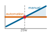
Cumulative manual work overtakes the one-time automation investment near week 20.

Manual operations hit a capacity ceiling, but the cost problem extends beyond engineering time. ML systems accumulate hidden complexity through specific debt patterns, each emerging from ML’s distinctive reliance on data rather than deterministic logic, statistical rather than exact behavior, and implicit dependencies through data flows rather than explicit interfaces.

\scalebox{0.73}{%
\begin{tikzpicture}[line join=round,font=\small\sffamily]
\tikzset{%
planet/.style = {circle, draw=none,
semithick, fill=blue!30,
                    font=\sffamily\bfseries, ball color=green!70!blue!70,shading angle=-15,
                    text width=27mm, inner sep=1mm,align=center},
satellite/.style = {circle, draw=#1, semithick, fill=#1!30,
                    text width=18mm, inner sep=1pt, align=flush center,minimum size=21mm},%<---
arr/.style = {-{Triangle[length=3mm,width=6mm]}, color=#1,
                    line width=3mm, shorten <=1mm, shorten >=1mm}
}
%planet
\node (p)   [planet]    {ML system};
%satellites
\foreach \i/\j [count=\k] in {red/{Machine Resource Management},
cyan/{Configuration},
purple/{Data Collection},
green/{Data Verification},
orange/{Serving Infrastructure},
yellow/{Monitoring},
Siva/{Feature Extraction},
magenta/{ML Code},
violet/{Analysis Tools},
teal/{Process Management Tools}
}
%connections
{
\node (s\k) [satellite=\i,font=\footnotesize\sffamily] at (\k*36:3.8) {\j};
\draw[arr=\i] (p) -- (s\k);
}
\end{tikzpicture}}

Figure 2: Hidden Infrastructure of ML Systems: ML code is one of ten components arranged around the ML system at the center, alongside data collection, data verification, feature extraction, configuration, machine resource management, serving infrastructure, monitoring, analysis tools, and process management tools. The count is what matters, since modeling occupies one box and the remaining nine are the operational surface a deployment must also carry. Source: (Sculley et al. 2015).

Napkin Math 1.1: The cumulative cost of manual operations

Problem: Why build automated pipelines when manual retraining is faster?

Physics: Manual work accumulates over time.

Manual retrain: 4 hours of engineering per week.
Pipeline build: 80 engineering hours (one-time).

Math:

Result: 80 engineering hours $\div$ 4 hours per week = 20 weeks.
Trap: This assumes the model never changes.
Limitation: Additional features can increase manual effort.
Consequence: After 1 year, manual teams still spend 4 hours per week on maintenance. In this simplified calculation, pipeline teams incur 0 recurring hours.

Context: A central law of systems engineering is that the cost of maintaining a system over its lifetime can dominate the cost of building it. In ML, technical debt is especially dangerous because it is often data-driven rather than code-driven: a perfect piece of code can still fail if the data it processes shifts. Measurement is the management boundary: without telemetry, the team cannot tell whether maintenance work is reducing debt or merely hiding it.

Systems insight: Automation addresses capacity limits, not speed alone. A manual team eventually reaches a point where maintaining existing models prevents it from deploying new ones. MLOps responds with systematic observability and automation. Without monitoring infrastructure to make silent failures visible, the team accumulates debt and builds a system that becomes increasingly difficult to manage.

Figure 3 maps six patterns across data, model, and infrastructure concerns. The representative examples that follow connect each pattern to the engineering response it demands.

\scalebox{0.75}{%
\begin{tikzpicture}[line join=round,font=\small\sffamily]
\tikzset{%
planet/.style = {circle, draw=none,semithick, fill=RedLine!30,
                    font=\sffamily\bfseries,
                    text width=27mm, inner sep=1mm,align=flush center},
satellite/.style = {rectangle, draw=#1, semithick, fill=#1!20,
                    text width=18mm, inner sep=1pt, align=flush center,minimum size=21mm,minimum height=10mm},
satellite1/.style = {rectangle, draw=#1, semithick, fill=#1,anchor=east,
                   inner sep=1pt, align=flush center,minimum size=2.5mm,minimum height=10mm},
arr/.style = {-{Triangle[length=3mm,width=6mm]}, color=#1,
                    line width=3mm, shorten <=1mm, shorten >=1mm},
TxtL/.style = {font=\footnotesize\sffamily,text width=30mm,align=flush right},
TxtR/.style = {font=\footnotesize\sffamily,text width=30mm,align=flush left},
TxtC/.style = {font=\footnotesize\sffamily,text width=30mm,align=flush center}
}
%planet
\node (p)   [planet]    {Hidden Technical Debt};
%satellites
\foreach \i/\j/\radius/\sho [count=\k] in {
  red/{Configuration Debt}/3.1/7pt,
  cyan/{Feedback Loops}/3.1/7pt,
  Siva/{Data Debt}/4.0/10pt,
  green!65!black/{Pipeline Debt}/3.1/7pt,
  orange/{Correction Cascades}/3.1/7pt,
  yellow!80!red/{Boundary Erosion}/4.1/10pt
}
{
%Satelit
\node (s\k) [satellite=\i,font=\footnotesize\sffamily] at (\k*60:\radius) {\j};
%Decoration
\node[satellite1=\i](DE\k) at (s\k.west) {};
%Arrows
\draw[arr=\i,shorten >=\sho] (p) -- (s\k);
}
\node[TxtL,left=2pt of DE2]{\textbf{Undeclared Consumers:} Hidden model dependencies};
\node[TxtR,right=2pt of s1.east,anchor=west]{\textbf{Parameter Sprawl:}\\ Ad hoc settings and
hard-coded values};
\node[TxtL,left=2pt of DE4]{\textbf{Fragile Workflows:} Tightly coupled};
\node[TxtR,text width=40mm,right=2pt of s5.east,anchor=west]{\textbf{Sequential Dependencies:}
Upstream fixes break downstream systems};
\node[TxtL,left=10pt of s3]{\textbf{Quality Issues:} Inconsistent formats
and distributions};
\node[TxtR,right=2pt of s6]{\textbf{CACE Principle:}
Change Anything Changes Everything};
\end{tikzpicture}}

Figure 3: ML Technical Debt Taxonomy: Six debt patterns radiate from hidden technical debt: configuration debt, feedback loops, data debt, pipeline debt, correction cascades, and boundary erosion. The surrounding labels identify their associated failure patterns.

Boundary erosion

The first and often most insidious debt pattern involves the dissolution of system boundaries. In traditional software, modularity and abstraction provide clear boundaries between components, allowing changes to be isolated and behavior to remain predictable. Machine learning systems blur these boundaries for a structural reason: model behavior depends on statistical properties of data flowing through the system rather than on explicit interfaces. A change to upstream data formatting might pass all unit tests while silently degrading downstream model accuracy. This implicit coupling through data, rather than code, creates tightly coupled interactions between data pipelines, feature engineering, model training, and downstream consumption.

This erosion produces entanglement: dependencies between components become so intertwined that local modifications require global understanding and coordination. The result is captured by the CACE principle: Change Anything Changes Everything. When systems lack strong boundaries, adjusting a feature encoding, model hyperparameter, or data selection criterion can affect downstream behavior in unpredictable ways. For example, changing the binning strategy of a numerical feature may cause a previously tuned model to underperform, triggering retraining and downstream evaluation changes that ripple far beyond the original modification.

The primary defense against boundary erosion is architectural: modularity and encapsulation at the design level. Components with well-defined interfaces allow engineers to isolate faults, reason about changes, and reduce the risk of system-wide regressions. Explicit separation between data ingestion, feature engineering, and modeling logic introduces layers that can be independently validated, monitored, and maintained. Boundary erosion is often invisible in early development because the tight coupling only becomes apparent when a seemingly local change triggers a distant failure. Proactive design decisions that preserve abstraction, systematic testing, and interface documentation provide the most practical defenses against this creeping complexity.

Correction cascades

If boundary erosion describes how ML systems lose their structural integrity, correction cascades describe what happens when teams attempt repairs. A correction cascade occurs when fixing one component introduces problems elsewhere, requiring additional fixes that themselves cause further problems. In ML systems, these cascades are particularly severe because changes propagate through statistical dependencies rather than explicit code paths. Retraining a model to fix one failure mode may degrade performance on previously working cases. Adjusting thresholds to reduce false positives may increase false negatives. Adding features to address edge cases may introduce correlations that destabilize the entire system. Each correction triggers the need for more corrections, creating a cascade that can consume engineering resources far exceeding the original fix.

Figure 4 makes the cascade structure visible as a chain of dependent models. Each model is trained to correct the errors of the one before it: model B compensates for model A’s residual mistakes, model C compensates for model B’s, and so on down the chain. The arrangement holds until an upstream model changes. When model A is retrained to fix one failure mode, every downstream model that was tuned to its previous behavior is invalidated at once, and each must be re-corrected. The red arcs trace this propagation, showing how a repair that looked local reaches across the entire chain. A change near the top forces the most rework, while one near the bottom is nearly free. For an operations team, one change request can trigger a coordinated retraining of the chain.

\begin{tikzpicture}[font=\small\sffamily, >=stealth]
\tikzset{
Line/.style={line width=0.5pt,black!50,text=black},
LineA/.style={-{Triangle[width=7pt,length=11pt]},line width=1pt,black!50,text=black},
LineD/.style={-{Triangle[width=7pt,length=11pt]},crimson,line width=1.5pt,rounded corners=15pt,
dashed,dash pattern=on 7pt off 5pt},
Box/.style={align=center, inner xsep=2pt,draw=none, line width=1pt,fill=none,
minimum width=30mm, minimum height=25mm,node distance=1.0},
Box1/.style={align=center, inner sep=5pt,draw=none, line width=1pt,fill=crimson,text=white,
 minimum width=18mm, minimum height=7mm,font=\small\sffamily\bfseries,rounded corners=7pt},
Text2/.style={font=\sffamily\bfseries\small,align=center},
Text3/.style={font=\sffamily\bfseries\small,align=center,redd},
}
\definecolor{redd}{HTML}{A31F34}
\definecolor{blueeD}{HTML}{4A90C4}
\definecolor{blueeL}{HTML}{CFE2F3}

%model
\tikzset{%
 pics/model/.style = {
        code = {
        \pgfkeys{/channel/.cd, #1}
\begin{scope}[local bounding box=MODEL,scale=\scalefac, every node/.append style={transform shape}]
\foreach \i in {1,...,3}{
  \pgfmathsetmacro{\y}{(-\i)*0.37}
  \node[circle,draw, minimum size=2.5mm,inner sep=0pt,fill=red](2K\i) at(0,\y){};
}
\foreach \i in {1,...,3}{
  \pgfmathsetmacro{\y}{(-\i)*0.37}
  \node[circle,draw, minimum size=2.5mm,inner sep=0pt,fill=brown](3K\i) at(0.6,\y){};
}
\foreach \i in {1,...,2}{
  \pgfmathsetmacro{\y}{-(3.5-\i)*0.37}
  \node[circle,draw, minimum size=2.5mm,inner sep=0pt,fill=cyan](1K\i) at(-0.6,\y){};
}
\foreach \i in {1}{
  \pgfmathsetmacro{\y}{-(3.0-\i)*0.37}
  \node[circle,draw, minimum size=2.5mm,inner sep=0pt,fill=green!40!black](4K\i) at(1.2,\y){};
}
\foreach \i in {1,...,2}{
  \foreach \j in {1,...,3}{
\draw[Line](1K\i)--(2K\j);
}}
\foreach \i in {1,...,3}{
  \foreach \j in {1,...,3}{
\draw[Line](2K\i)--(3K\j);
}}\foreach \i in {1,...,3}{
  \foreach \j in {1}{
\draw[Line](3K\i)--(4K\j);
}}
 \end{scope}
     }
  }
}
\pgfkeys{
  /channel/.cd,
  scalefac/.store in=\scalefac,
  scalefac=1,
}

\begin{scope}[local bounding box=mainfig]
%Models
\foreach \name/\x/\title/\subtitle/\picid in {
  B1/0/{Model A}/{base predictions}/1,
  B2/6/{Model B}/{corrects A}/2,
  B3/12/{Model C}/{corrects B}/3,
  B4/18/{Model D}/{corrects C}/4
}{
  % osnovni box
  \node[Box] (\name) at (\x,0) {};

  % gornji i donji fill
  \fill[cyan!07] (\name.north west)
    rectangle ($( \name.north east)!0.6!(\name.south east)$)
    coordinate (\name DE);

  \fill[cyan!20] (\name.south east)
    rectangle ($( \name.north west)!0.6!(\name.south west)$)
    coordinate (\name LE);

  % spoljašnja linija / border
  \node[Box,draw=blueeD] at (\name.center) {};

  % tekst u box-u
  \node[Text2] at ($(\name.south west)!0.5!(\name DE)$)
    {\title\\
    \textcolor{black!70}{\sffamily\subtitle}};

  % koordinata za ikonicu / pic
  \coordinate (\name Q) at ($(\name.north west)!0.5!(\name DE)$);

  % pic
  \pic[shift={(-0.3,0.73)}] at (\name Q)
    {model={scalefac=1.0}};
}
%%%
\foreach \x in {2,3,4}{
\node[below=3pt of B\x.south,Text3]{must re-correct};
}
%
\draw[LineD](B1.north)--++(0,17.8mm)-|(B4.north);
\draw[LineD](B1.north)--++(0,14.0mm)-|(B3.north);
\draw[LineD](B1.north)--++(0,10.5mm)-|(B2.north);
%
\node[Box1,above=5pt of B1.north]{change};
\end{scope}

\draw[LineA](B1)--(B2);
\draw[LineA](B2)--(B3);
\draw[LineA](B3)--(B4);
%
\node[below =8mm of mainfig.south,font=\small\sffamily\itshape,
black!70]{A single fix to an upstream model forces every
downstream correction to be redone.};

\coordinate(L1)at($(B2.south)+(-6mm,-11mm)$);

\begin{scope}[local bounding box=MC,shift={($(L1)+(0,0)$)}]
\node[](LT1) at(L1){correction dependency};
\draw[LineA](LT1.west)+(180:15mm)--(LT1.west);

\node[right=49mm of LT1](LT2) at(L1){change propagates downstream};
\draw[LineD](LT2.west)+(180:15mm)--(LT2.west);
\end{scope}
\end{tikzpicture}

Figure 4: Correction Cascades: Each model is trained to correct the errors of the model before it, forming a chain of dependencies. Changing an upstream model invalidates every downstream correction at once, turning one local fix into cascading rework across the chain, with each downstream fix demanding its own retraining cycle.

Those arcs matter because they turn local repairs into lifecycle-wide dependencies. Sequential model development is one common source: reusing or fine-tuning existing models accelerates development for new tasks, but it also creates hidden assumptions that are difficult to unwind later. Assumptions embedded in earlier models become implicit constraints for future models, limiting flexibility and increasing the cost of downstream corrections.

Consider a team that fine-tunes a customer churn prediction model for a new product. The original model may embed product-specific behaviors or feature encodings that do not transfer to the new setting. As performance issues emerge, teams may attempt to patch the model, only to discover that the true problem lies several layers upstream in the original feature selection or labeling criteria.

To mitigate correction cascades, teams must balance reuse against redesign. Fine-tuning can reduce computation and data requirements, but it also inherits assumptions from the source model. Training from scratch offers greater control over those assumptions at a much higher data and compute cost. Dataset size alone does not decide between them; task similarity, source-model fit, available data, compute budget, and the cost of inherited dependencies do.

The underlying mechanism is that when model A’s outputs influence model B’s training data, implicit dependencies emerge through data flows rather than explicit code interfaces. These dependencies are invisible to traditional dependency analysis tools. Preventing cascades requires architectural decisions that preserve system modularity: keeping models loosely coupled, maintaining clear version boundaries, and designing for independent evolution even when reusing components.

Interface and dependency challenges

Boundary erosion and correction cascades both arise when ML systems develop interface dependencies that bypass explicit interfaces. Traditional software dependencies are visible (import statements, API calls, configuration files) and can be analyzed by tools. ML dependencies hide in data. When model A’s predictions become features for model B, the dependency exists only in the data pipeline, invisible to code analysis. When a dashboard consumes model outputs to drive business decisions, no interface contract governs the relationship.

Two critical patterns illustrate these challenges. Undeclared consumers arise when model outputs serve downstream components without formal tracking or interface contracts. When models evolve, these hidden dependencies break silently. A credit scoring model’s outputs might feed an eligibility engine that influences future applicant pools and training data, creating untracked feedback loops that bias model behavior over time. Data dependency debt compounds this problem as ML pipelines accumulate unstable and underutilized data dependencies that become difficult to trace or validate. Feature engineering scripts, data joins, and labeling conventions lack the dependency analysis tools available in traditional software development. When data sources change structure or distribution, downstream models fail unexpectedly.

Mitigating these interface challenges requires systematic approaches: strict access controls for model outputs, formal interface contracts with documented schemas, data versioning and lineage tracking systems, and continuous monitoring of prediction usage patterns. The MLOps infrastructure patterns presented in subsequent sections provide concrete implementations of these solutions.

System evolution challenges

The debt patterns in section 1.3.3 describe poor design choices. Even well-designed ML systems face evolution challenges that differ sharply from traditional software.

Feedback loops represent the most subtle evolution challenge: models influence their own future behavior through the data they generate. Recommendation systems exemplify this dynamic: suggested items shape user clicks, which become training data, potentially creating self-reinforcing biases. Operationally, the warning sign is a subgroup error gap that widens across retraining cycles: one cohort receives worse predictions, those predictions reshape future behavior or labels, and the next dataset amplifies the gap. The MLOps lesson is to monitor cohorts before aggregate metrics hide the loop. These loops undermine data independence assumptions and can mask performance degradation for months.

Pipeline and configuration debt accumulates as ML workflows evolve into “pipeline jungles” of ad hoc scripts and fragmented configurations. Without modular interfaces, teams build duplicate pipelines rather than refactor brittle ones, leading to inconsistent processing and growing maintenance burden. Compounding this, rapid prototyping encourages embedding business logic in training code and undocumented configuration changes. While these early-stage shortcuts are necessary for innovation, they become liabilities as systems scale across teams. Managing evolution requires architectural discipline: cohort-based monitoring for loop detection, modular pipeline design with workflow orchestration tools, and treating configuration as a first-class system component with versioning and validation.

Code and architecture debt

Data dependencies and system evolution create debt through implicit coupling. ML systems also accumulate code-level debt patterns that differ from traditional software. Sculley et al. (2015) identify several that deserve explicit attention.

Glue code dominates ML codebases: systems often require substantial integration code to connect general-purpose ML packages to specific data pipelines and serving systems, with the glue constituting up to 95 percent of the codebase while the actual ML code represents only 5 percent. This glue creates tight coupling between package APIs and the surrounding system, meaning that when packages update their interfaces, all glue code must be rewritten. Mitigation requires wrapping ML packages in stable internal APIs and treating external dependencies as substitutable components.

Dead experimental codepaths accumulate as ML development involves extensive experimentation, leaving behind conditional branches for abandoned approaches. Unlike traditional dead code that can be detected statically, experimental ML codepaths often remain “live” because they are controlled by configuration flags rather than compile-time conditions. Over time, these paths increase testing burden and create confusion about which code actually runs in production. Regular code audits with explicit deprecation timelines and feature flag hygiene help manage this debt.

Abstraction debt arises because traditional software engineering relies on well-defined abstractions like functions, classes, and modules, but ML systems lack mature abstractions for key concepts such as the right interface for a “feature” or the right encapsulation for “model behavior.” This absence forces teams to reinvent abstractions or, worse, avoid abstraction entirely. Common patterns such as feature stores (abstracting feature computation), model registries (abstracting model versioning), and prediction services (abstracting inference) reduce per-project abstraction debt when they fit the team’s workflow.

Beyond these patterns, Sculley et al. (2015) identify warning signs, or common smells, that indicate accumulating debt: the Plain-Old-Data Type Smell (using generic types like strings and floats instead of semantic types that encode meaning and constraints), the Multiple-Language Smell (systems spanning Python, SQL, C++, and shell scripts with inconsistent conventions), and the Prototype Smell (“temporary” research code that becomes permanent infrastructure without refactoring). Effective organizations track these smells in code reviews and allocate explicit time for debt reduction, treating technical debt paydown as a first-class engineering activity rather than an afterthought.

Technical debt in practice

The debt patterns described earlier are not theoretical constructs. They have played a critical role in shaping real-world machine learning systems. In practice, unseen dependencies and misaligned assumptions can accumulate quietly, only to become major liabilities over time.

Production debt patterns

The first pair exposes coupling through model behavior. YouTube’s recommendation system illustrates how large recommenders learn from noisy user-behavior signals, making ranking objectives, equal per-user weighting, and live A/B evaluation part of the system design rather than offline evaluation details (Covington et al. 2016). Zillow’s home valuation and purchasing workflow exposed the correction-cascade version during its iBuying venture.⁶ Valuation and inventory assumptions propagated into purchasing decisions; later corrections then destabilized inventory and pricing decisions, forcing revalidation and eventually a full rollback when the company shut down the iBuying arm in 2021.

Covington, Paul, Jay Adams, and Emre Sargin. 2016. “Deep Neural Networks for YouTube Recommendations.” Proceedings of the 10th ACM Conference on Recommender Systems, 191–98. https://doi.org/10.1145/2959100.2959190.

⁶ Zillow iBuying failure: Zillow reported a plan to wind down Zillow Offers in November 2021, including a Q3 inventory write-down and workforce reductions (Zillow Group 2021). The failure illustrates correction cascade debt at scale: pricing errors, purchasing decisions, and inventory feedback can reinforce one another, creating a loop that no single retraining cycle can break.

Zillow Group. 2021. Zillow Group Reports Third-Quarter 2021 Financial Results and Shares Plan to Wind down Zillow Offers Operations. Investor Relations Press Release.

National Transportation Safety Board. 2017. Collision Between a Car Operating with Automated Vehicle Control Systems and a Tractor-Semitrailer Truck Near Williston, Florida, May 7, 2016. HAR-17/02. National Transportation Safety Board.

Engineering, M. 2016. Introducing FBLearner Flow: Facebook’s AI Backbone. Engineering at Meta Blog.

Mosseri, Adam. 2018. Bringing People Closer Together. Meta Newsroom.

The second pair exposes coupling through ownership and configuration. Safety-critical driving automation illustrates the undeclared-consumer risk from a different direction: when automated-control outputs, driver expectations, and subsystem responsibilities are not specified clearly enough, operational failures can cross component boundaries rather than staying local (National Transportation Safety Board 2017). Facebook’s News Feed iterations show the configuration version of the same governance problem. Rapid experimentation and ranking changes require traceable settings and explicit objectives; otherwise behavioral changes become hard to audit after deployment (Engineering 2016; Mosseri 2018).

These examples are not cautionary tales from careless organizations. They are predictable consequences of deploying probabilistic or automated decision systems without infrastructure that makes coupling visible. YouTube, Zillow, safety-critical driving automation, and Facebook each expose a different debt pattern: feedback loops, correction cascades, undeclared consumers, and configuration sprawl.

Each debt pattern suggests corresponding controls: feature stores can reduce data dependency debt, versioning systems expose configuration debt, CI/CD pipelines constrain pipeline debt, and monitoring systems make feedback loops visible. These are not one-to-one cures but engineering responses to the failure modes diagnosed earlier. Recognizing debt patterns, however, is only half the battle: the organizations in these case studies did not lack talented engineers, but rather lacked systematic controls that could catch specific problems before they compounded. The transition from diagnosis to prevention requires examining each infrastructure component in detail: understanding what it does and, more critically, how it addresses the failure mode that motivated its creation.

Self-Check: Question

According to Sculley et al. (2015), why is technical debt in machine learning systems fundamentally more challenging to detect and manage than conventional software debt?
1. Because ML frameworks prevent developers from running unit tests or continuous integration jobs
2. Because ML algorithms require more lines of raw mathematical code than supporting infrastructure software
3. Because ML debt accumulates through implicit statistical relationships, data dependencies, and feedback loops that degrade predictive accuracy silently without throwing runtime exceptions
4. Because neural network parameters cannot be serialized to disk or stored in artifact registries
A data engineering team spends 6 hours per week manually extracting features, executing training runs, and validating a customer churn model. Building an automated CI/CD retraining pipeline requires a one-time upfront investment of 120 engineering hours. What is the breakeven time for this automation investment, and what long-term capacity risk arises if the team remains manual?
1. Breakeven is 6 weeks; manual processes remain more cost-effective for multi-model deployments
2. Breakeven is 10 weeks; automated pipelines eliminate the need for future model monitoring
3. Breakeven is 40 weeks; manual maintenance has zero ongoing engineering cost after the first year
4. Breakeven is 20 weeks; manual maintenance scales linearly with the number of deployed models until engineering capacity is fully consumed by routine operations
Explain why ‘correction cascades’ create a severe maintenance trap in production ML architectures, and state the primary architectural remedy.
True or False: In production ML systems, ‘glue code’ refers to the core machine learning algorithm, which typically comprises over 90% of the total system codebase.
The systemic vulnerability where modifying a single input feature’s distribution or encoding alters the learned weights and contributions of all other features across an ML pipeline is known as the ____ principle.

See Answers →

Development Infrastructure

Development infrastructure turns the debt patterns diagnosed earlier into enforcement points. A feature schema that drifts upstream cannot be repaired by a dashboard alone; it needs a shared contract, a versioned artifact, and a deployment path that rejects incompatible changes before they reach production. Table 6 maps each component directly to a foundational principle (section 1.2.1) and a specific failure mode.

Table 6: MLOps Infrastructure as Debt Remediation: Each infrastructure component responds to a class of technical debt observed in production ML systems. Feature stores can reduce training-serving skew by reusing feature definitions and values; versioning systems support reproducibility; CI/CD pipelines automate rollout controls; monitoring systems can surface silent degradation before users do.

Infrastructure Component	Principle Implemented	Debt Pattern Addressed
Feature stores	Consistency Imperative	Data dependency debt, training-serving skew
Versioning systems	Reproducibility Through Versioning	Configuration debt, correction cascades
CI/CD pipelines	Cost-Aware Automation	Pipeline debt, boundary erosion
Monitoring systems	Observable Degradation	Feedback loops, silent failures

Figure 5 organizes these components across ML models, frameworks, orchestration, infrastructure, and hardware. Understanding how these layers interact enables practitioners to design systems that systematically address the technical debt patterns identified earlier while maintaining operational sustainability.

\begin{tikzpicture}[line width=0.75pt,font=\small\sffamily]
%
\tikzset{%
   Line/.style={line width=1.0pt,GrayLine},
   Box/.style={align=flush center,
    inner xsep=2pt,
    node distance=0.9,
    draw=BlueLine,
    line width=0.75pt,
    fill=BlueFill,
    text width=31mm,
    minimum width=31mm, minimum height=10mm
  },
  Box2/.style={Box,text width=40mm,minimum width=40mm,fill=OrangeFill,draw=OrangeLine
  },
Box3/.style={Box, fill=GreenFill,draw=GreenLine},
Box31/.style={Box3, node distance=0.5, minimum height=9mm},
Box4/.style={Box, fill=RedFill,draw=RedLine,text width=34mm, minimum width=34mm},
Box41/.style={Box4, node distance=0.5, minimum height=9mm},
}
%
\node[Box,text width=37mm, minimum width=37mm](B1){\textbf{ML Models/Applications} (e.g., BERT)};
\node[Box2,right=0.35 of B1](B2){\textbf{ML Frameworks/Platforms} (e.g., PyTorch)};
\node[Box3,right=of B2](B3){\textbf{Model Orchestration} (e.g., Ray)};
\node[Box4,right=0.4of B3](B4){\textbf{Infrastructure}\\ (e.g., Kubernetes)};
\node[Box,right=of B4,fill=VioletFill,draw=VioletLine](B5){\textbf{Hardware}\\ (e.g., a GPU cluster)};
%
\node[Box31,below=of B3](B31){Data Management};
\node[Box31,below=of B31](B32){CI/CD};
\node[Box31,below=of B32](B33){Model Training};
\node[Box31,below=of B33](B34){Model Eval};
\node[Box31,below=of B34](B35){Deployment};
\node[Box31,below=of B35](B36){Model Serving};
%
\node[Box41,below=of B4](B41){Job Scheduling};
\node[Box41,below=of B41](B42){Resource Management};
\node[Box41,below=of B42](B43){Capacity Management};
\node[Box41,below=of B43](B44){Monitoring};
\node[Box41,draw=none,fill=none,below=of B44](B45){};
\scoped[on background layer]
\node[draw=BackLine,inner xsep=11,inner ysep=19,yshift=3mm,fill=BackColor!70,fit=(B3)(B44)(B36),line width=0.75pt](BB1){};
\node[below=3pt of BB1.north, anchor=north]{MLOps};
%
\foreach \y in{3,4}{
\foreach \x in{1,2,3,4}{
\pgfmathtruncatemacro{\newX}{\x + 1}
\draw[-latex,Line](B\y\x)--(B\y\newX);
}}
\foreach \y in{3,4}{
\draw[-latex,Line](B\y)--(B\y1);
}
\draw[-latex,Line](B35)--(B36);
\draw[-latex,Line](B44)--(B45)coordinate(T44);

\node[inner sep=0pt,below=0 of T44,rotate=90,align=center,font=\tiny\sffamily]{$\bullet$ $\bullet$ $\bullet$};
%
\foreach \y in{1,2,3,4}{
\pgfmathtruncatemacro{\newX}{\y + 1}
\draw[Line](B\y)--(B\newX);
}
\end{tikzpicture}

Figure 5: MLOps Stack Layers: Five columns organize the ML system stack: ML Models/Applications, ML Frameworks/Platforms, Model Orchestration, Infrastructure, and Hardware. MLOps spans orchestration tasks from data management through model serving and infrastructure tasks from job scheduling through monitoring, supporting automation, reproducibility, and scalable deployment.

Data infrastructure and preparation

Reliable machine learning systems depend on structured, scalable, and repeatable data handling. From ingestion to inference, each stage must preserve quality, consistency, and traceability across initial development, continual retraining, auditing, and serving alike. These requirements demand systems that formalize data transformation and versioning throughout the ML lifecycle.

Data management

The technical debt patterns described earlier stem largely from poor data management: unversioned datasets create boundary erosion, inconsistent feature computation causes correction cascades, and undocumented data dependencies breed hidden consumers. Data management infrastructure directly addresses these root causes. Building on the data engineering foundations from Data Engineering, data collection, preprocessing, and feature transformation become formalized operational processes. Where data engineering focuses on single-pipeline correctness, MLOps data management emphasizes cross-pipeline consistency, ensuring that training and serving compute identical features. Data management thus extends beyond initial preparation to encompass the continuous handling of data artifacts throughout the ML system lifecycle.

Three principles organize the infrastructure that addresses these root causes: consistency, freshness, and quality. Each principle motivates specific tooling rather than the reverse.

The first requirement is data consistency: every artifact influencing model behavior, from raw datasets to engineered features, must be versioned and reproducible. Without versioning, teams cannot trace which data produced which model, making debugging and rollback impossible. The implementation usually combines code versioning, dataset versioning, and durable object storage. DVC (Data Version Control) (Iterative 2024), Git (Torvalds and Hamano 2024), Amazon S3 (Amazon Web Services 2024a), and Google Cloud Storage (Google Cloud 2024b) are examples of that pattern, but the invariant is the important part: raw and processed artifacts must remain addressable by version. Section 1.4.1.3 examines implementation details including Git integration, metadata tracking, and lineage preservation. At the feature level, a feature store can reduce skew by centralizing feature definitions and serving paths across training and serving pipelines, but parity still requires validation. Uber’s Michelangelo platform popularized this pattern inside a large production ML platform, and Feast later made the pattern available as open-source feature-store infrastructure (Hermann and Del Balso 2017; Gojek and Google 2019). Section 1.4.1.2 details implementation patterns for training-serving consistency.

Amazon Web Services. 2024a. Amazon Simple Storage Service (S3).

Google Cloud. 2024b. Google Cloud Storage.

Apache Software Foundation. 2024. Apache Airflow.

dbt Labs. 2024. Dbt (Data Build Tool).

Consistency alone is insufficient if the underlying data is stale. Data freshness ensures that models train and serve on current data rather than outdated snapshots. Automated data pipelines maintain freshness by continuously transforming raw data into analysis-ready formats through structured stages: ingestion, schema validation, deduplication, transformation, and loading. Workflow orchestrators such as Apache Airflow (Apache Software Foundation 2024) and Prefect (Prefect Technologies, Inc. 2024), together with the transformation framework dbt (dbt Labs 2024), make those stages explicit, schedulable, and reviewable as code. Once the pipeline is managed this way, data flows can evolve with model requirements without losing versioning, modularity, or CI/CD integration.

The third pillar, data quality, governs whether the data reaching models is accurate, complete, and consistently labeled. In supervised learning pipelines, labeling quality directly determines model ceilings. Labeling tools such as Label Studio (HumanSignal 2024) support scalable, team-based annotation with integrated audit trails and version histories, capabilities that become essential when labeling conventions evolve over time or require refinement across multiple project iterations.

HumanSignal. 2024. Label Studio: Open Source Data Labeling Platform.

To illustrate how these three principles reinforce each other in practice, consider a predictive maintenance application in an industrial setting. A continuous stream of sensor data is ingested and joined with historical maintenance logs through a scheduled pipeline managed in Airflow (freshness). The resulting features, including rolling averages and statistical aggregates, are stored in a feature store for both retraining and low-latency inference (consistency). Schema validation, sensor-range checks, missingness tests, and label audits catch malformed or unreliable maintenance records before they reach training (quality), while versioning and model-registry integration preserve traceability from data to deployed model predictions. Data management, organized around these three principles, establishes the operational backbone for model reproducibility, auditability, and sustained deployment at scale.

Feature stores

The data dependency debt and training-serving skew patterns described in section 1.3 share a common root cause: inconsistent feature computation across pipeline stages. Consider what typically happens without a feature store: a data scientist computes user_session_length in Python for training, while an engineer reimplements the same calculation in Java for serving. Subtle differences emerge: one uses wall-clock time, the other processing time; one includes idle timeouts, the other does not. The model trains on one definition but serves using another, and accuracy degrades silently. Feature stores⁷ address this challenge by providing an abstraction layer between data engineering and machine learning, implementing the consistency imperative through a single source of truth for feature values. In conventional pipelines, feature engineering logic is duplicated or diverges across environments, introducing risks of training-serving skew, data leakage, and model drift.

⁷ Feature store: Uber’s Michelangelo platform described a centralized feature store for sharing and serving features across production models (Hermann and Del Balso 2017). At that scale, the consistency guarantee must hold under an online latency budget: what distinguishes a feature store from a shared library of feature code is that the shared feature path also has to serve fresh features fast enough for real-time inference.

Hermann, Jeremy, and Mike Del Balso. 2017. Meet Michelangelo: Uber’s Machine Learning Platform. Uber Engineering Blog.

Feature stores manage both offline (batch) and online (real-time) feature access through a centralized repository. During training, features are computed and stored in a batch environment alongside historical labels. At inference time, corresponding transformation logic is applied to fresh data in an online serving system. This architecture can help models consume consistent features in both contexts, but teams must still test point-in-time correctness, freshness, and online-offline parity. The feature store is, in systems terms, an engineering mechanism that helps control training-serving skew: by centralizing feature definitions and serving them through a shared path, it reduces one source of the pipeline divergence that can cause silent production accuracy loss.

Beyond consistency, feature stores support versioning, metadata management, and feature reuse across teams. A fraud detection model and a credit scoring model may rely on overlapping transaction features that can be centrally maintained, validated, and shared. Integration with data pipelines and model registries enables lineage tracking: when a feature is updated or deprecated, dependent models are identified and retrained accordingly.

Training-serving skew: Diagnosis and prevention

Training-serving skew (defined formally in Training-serving skew) manifests operationally through feature store inconsistencies and pipeline divergence. Table 7 summarizes common causes and their detection methods:

Table 7: Training-Serving Skew Categories: Each category requires different detection and prevention strategies. Schema and preprocessing skew emerge from code divergence and require parity validation; shared feature logic, including a feature store where appropriate, can reduce them, while data distribution skew requires statistical monitoring against training baselines. Timing skew demands careful analysis of feature freshness between training and serving contexts.

Skew Type	Example	Detection Method
Feature preprocessing	Normalization uses different statistics	Statistical comparison of feature distributions
Missing data handling	Training fills NaN with mean; serving uses 0	Schema validation with explicit null handling
Time-dependent features	Features computed with different time cutoffs	Timestamp validation in feature pipelines
Library version drift	NumPy or Pandas version differences	Environment hash comparison

Training-serving skew case study

A practical example illustrates how training-serving skew manifests in production systems. Consider a recommendation system that shows 8 percent accuracy degradation one month after deployment with no model-code changes. Feature distribution comparison reveals that user_session_length has a mean of 45 minutes in training but 12 minutes in serving. The root cause is feature-definition skew: the offline training pipeline computes wall-clock duration from the first event to the last event in a session, while the online serving path counts only foreground-active time after idle gaps are removed. As a result, the model learned thresholds tied to a feature definition that production never actually serves.

Feature stores (building on the data pipelines from Data Engineering) address this problem by centralizing feature definitions and serving paths for training and serving pipelines. Listing 1 demonstrates the pattern: training retrieves point-in-time historical features, serving retrieves current online features, and both calls resolve to the same versioned feature definition rather than duplicated code paths. Parity still requires validation.

Listing 1: Feature Store Consistency: Unified retrieval reduces training-serving skew by sharing versioned feature definitions across both pipelines.

feature_definitions = registry.load(version="2026-06-01")

training_features = feature_definitions.materialize_historical(
    entities=training_entities,
    at_event_time=True,
    names=["user.session_length", "user.purchase_history"],
)

serving_features = feature_definitions.lookup_online(
    entities=[{"user_id": 12345}],
    names=["user.session_length", "user.purchase_history"],
)

assert training_features.schema == serving_features.schema
assert (
    training_features.definition_hash
    == serving_features.definition_hash
)

By defining session_length once, training and serving share its logic; parity checks must still verify the resulting values. Centralized feature stores also support feature reuse and metadata tracking, which makes skew easier to detect and correct when a feature definition changes (Hermann and Del Balso 2017; Gojek and Google 2019).

Gojek, and Google. 2019. Feast: An Open Source Feature Store for Machine Learning. Google Cloud Blog.

As the consistency imperative quantified (section 1.2.1.3), skew-induced errors at production scale can translate to hundreds of thousands of dollars in annual cost. Feature stores can reduce this recurring leakage through infrastructure investment with measurable returns. The economics become operational only when shared definitions can serve many models and teams.

Example 1.1: Uber Michelangelo feature store

Scenario: Uber’s Michelangelo platform supported production models such as estimated time of arrival and used shared feature infrastructure across offline training and online prediction (Hermann and Del Balso 2017). Separate implementations of the same feature logic would create training-serving skew.

Diagnosis: A shared feature contract reduces the chance that batch and online pipelines interpret a feature differently, while separate offline and online stores still require point-in-time and parity validation.

Systems lesson: Feature stores reduce one major source of training-serving skew by centralizing versioned feature definitions and access paths. They do not eliminate skew: point-in-time correctness, freshness, and online-offline parity still require explicit tests.

Skew detection in CI/CD

Automated pipelines should validate feature consistency before deployment. Listing 2 shows a function that compares training and serving feature distributions using the Kolmogorov-Smirnov test, rejecting deployment when any feature diverges beyond a threshold. The gate converts an observable distribution mismatch into a CI failure before promotion, but its KS threshold must be calibrated to sample size and feature criticality; a passing statistic does not prove schema, semantic, or point-in-time parity.

Listing 2: Feature Skew Validation: This function compares training and serving feature distributions using the Kolmogorov-Smirnov test, rejecting deployment when any feature diverges beyond a configurable threshold.

def validate_no_skew(
    training_features, serving_features, threshold=0.1
):
    """Reject deployment if feature distributions diverge."""
    for feature in training_features.columns:
        ks_stat = ks_2samp(
            training_features[feature], serving_features[feature]
        )
        if ks_stat.statistic > threshold:
            raise SkewDetectedError(
                f"{feature}: KS={ks_stat.statistic:.3f}"
            )

Versioning and lineage

Lineage tracking and versioning implement reproducibility (section 1.2.1), which requires all artifacts influencing model behavior to be versioned. Unlike traditional software, ML models depend on multiple changing artifacts: training data, feature engineering logic, trained model parameters, and configuration settings. MLOps practices enforce tracking of versions across all pipeline components to manage this complexity.

Data versioning allows teams to snapshot datasets at specific points in time and associate them with particular model runs, including both raw data and processed artifacts. Model versioning registers trained models as immutable artifacts alongside metadata such as training parameters, evaluation metrics, and environment specifications. Model registries⁸ provide structured interfaces for promoting, deploying, and rolling back model versions, with some supporting lineage visualization tracing the full dependency graph from raw data to deployed prediction (MLflow Project 2026; Google Cloud 2024d).

⁸ Model registry: Prevents “registry bypass,” the failure mode where the undocumented production model diverges from the trained artifact through different preprocessing, stale serialization formats, or manual hotfixes applied directly to the serving endpoint. Without a registry enforcing versioned, immutable artifacts with queryable metadata and state, rollbacks require locating the correct weights from an ad-hoc artifact store under incident pressure.

MLflow Project. 2026. MLflow Model Registry.

These complementary practices form the lineage layer of an ML system. The lineage layer enables introspection, experimentation, and governance by preserving the chain of evidence needed to diagnose a degraded model: whether the input distribution matched training data, whether feature definitions changed, and whether the deployed model version matched the serving infrastructure. By elevating versioning and lineage to first-class citizens in the system design, MLOps enables teams to build and maintain reliable, auditable, and evolvable ML workflows at scale.

Continuous pipelines and automation

Feature stores and versioning systems address data consistency statically: they ensure that features are computed correctly at a point in time. Automation enables these systems to evolve continuously, synchronizing data preprocessing, training, evaluation, and release into integrated workflows that respond to new data, shifting objectives, and operational constraints (Orr et al. 2021; Google Cloud 2026b).

Orr, Laurel, Atindriyo Sanyal, Xiao Ling, Karan Goel, and Megan Leszczynski. 2021. “Managing ML Pipelines: Feature Stores and the Coming Wave of Embedding Ecosystems.” Proceedings of the VLDB Endowment 14 (12): 3178–81. https://doi.org/10.14778/3476311.3476402.

CI/CD pipelines

Feature stores and versioning systems address the data side of consistency; CI/CD pipelines address the process side, ensuring that changes flow through validated stages rather than ad hoc deployments. ML CI/CD pipelines must handle complexity absent from traditional software: data dependencies, model training workflows, and artifact versioning that couple code changes to statistical behavior changes.

A typical ML CI/CD pipeline consists of coordinated stages: checking out updated code, preprocessing input data, training a candidate model, validating performance, packaging the model, and deploying to a serving environment. In some cases, pipelines also include triggers for automatic retraining based on data drift or performance degradation. By codifying these steps, CI/CD pipelines⁹ reduce manual intervention, enforce quality checks, and support continuous improvement of deployed systems.

⁹ Idempotency: This property ensures that retrying a pipeline stage does not create duplicate externally visible effects, conflicting registrations, or repeated deployment actions. Producing identical models from identical inputs is a separate property—determinism and reproducibility—and the training stage may violate it due to randomness such as weight initialization. Production systems therefore combine stable run identifiers and atomic publication for idempotency with fixed random seeds, deterministic kernels, fixed library versions, and controlled data ordering for reproducibility.

CircleCI. 2024. CircleCI: Continuous Integration and Delivery Platform.

GitHub, Inc. 2024b. GitHub Actions.

Authors, Kubeflow. 2024. Kubeflow.

Netflix. 2024. Metaflow.

Prefect Technologies, Inc. 2024. Prefect: Workflow Orchestration Framework for Python.

ML-focused CI/CD layers two tiers of tooling for one reason. A general-purpose CI/CD orchestrator (Jenkins, CircleCI (2024), or GitHub Actions (GitHub, Inc. 2024b)) manages version-control events and execution logic, but the ML layer must additionally version data, gate on model metrics, and trigger retraining. Teams therefore add an ML platform or workflow orchestrator (Kubeflow (Authors 2024), Metaflow (Netflix 2024), or Prefect (Prefect Technologies, Inc. 2024)) that supplies higher-level abstractions for those tasks.

Without this automation, model deployment degrades into a manual, error-prone process: an engineer retrains locally, copies artifacts to a staging server, and promotes to production with no guarantee that the data, code, or hyperparameters match what was validated. The cost of such ad hoc workflows compounds with team size and deployment frequency, producing configuration drift and silent regressions that surface only after the model has served incorrect predictions.

Figure 6 shows how a representative continuous-training pipeline moves from dataset ingestion and validation through transformation, training/tuning, evaluation, model validation, and model registration. A retraining trigger initiates the process, while dataset, model, metadata, and artifact repositories preserve the inputs and outputs needed for lineage.

\begin{tikzpicture}[line join=round,font=\small\sffamily]
\definecolor{Red}{RGB}{249,56,39}
\definecolor{Blue}{RGB}{0,97,168}
\definecolor{Violet}{RGB}{178,108,186}
\tikzset{%
helvetica/.style={align=flush center, font={\sffamily\small}},
cyl/.style={cylinder, draw=BrownLine,shape border rotate=90, aspect=1.8,inner ysep=0pt,
    minimum height=20mm,minimum width=21mm, cylinder uses custom fill,
 cylinder body fill=brown!10,cylinder end fill=brown!35},
Line/.style={line width=1.2pt,black!50},
LineB/.style={line width=1.5pt,BlueLine
   },
  Box/.style={align=flush center,
    inner xsep=2pt,
    node distance=0.9,
    draw=BlueLine,
    line width=0.75pt,
    fill=BlueL!80,
    text width=22mm,
    minimum width=22mm, minimum height=10mm
  },
Box2/.style={Box,fill=OrangeL,draw=OrangeLine},
Box3/.style={Box, fill=GreenL,draw=GreenLine},
Box4/.style={Box, fill=RedL,draw=RedLine},
}
\definecolor{CPU}{RGB}{0,120,176}

\node[Box](B1){Data validation};
\node[Box2,right=of B1](B2){Data transformation};
\node[Box3,right=of B2](B3){Model validation};
\node[Box4,right=of B3](B4){Model registration};
\node[Box,above=0.75 of B1](B11){Dataset ingestion};
\node[Box2,above=0.75 of B2](B21){Model training/tuning};
\node[Box3,above=0.75 of B3](B31){Model evaluation};
%fitting
\scoped[on background layer]
\node[draw=BackLine,inner xsep=11,inner ysep=19,yshift=3mm,
           fill=BackColor!70,fit=(B11)(B4),line width=0.75pt](BB1){};
\node[below=3pt of  BB1.north,anchor=north,helvetica]{\textbf{Continuous training pipeline}};

\draw[-latex,Line](B11)--(B1);
\draw[-latex,Line](B1)--(B2);
\draw[-latex,Line](B2)--(B21);
\draw[-latex,Line](B21)--(B31);
\draw[-latex,Line](B31)--(B3);
\draw[-latex,Line](B3)--(B4);
%cylinder left
\begin{scope}[local bounding box = CYL1,shift={($(BB1.west)+(-3.85,0)$)}]
\node (CA1) [cyl] {};
\node[align=center]at (CA1){Dataset \&\\ feature\\repository};
\end{scope}
%cylinder right
\begin{scope}[local bounding box = CYL2,shift={($(BB1.east)+(3.85,0)$)}]
\node (CA1) [cyl] {};
\node[align=center]at (CA1){Model\\repository};
\end{scope}
%cylinder top
\begin{scope}[local bounding box = CYL3,shift={($(BB1.north)+(0,2.4)$)}]
\node (CA1) [cyl] {};
\node[align=center]at (CA1){ML metadata\\\& artifact\\repository};
\end{scope}
% connect cube and fitting
\draw[{Circle[length=4.5pt]}-latex,LineB](CYL1.east)coordinate(CC1)--(CYL1.east-|BB1.west)coordinate(CC2);
\draw[latex-{Circle[length=4.5pt]},LineB](CYL2.west)coordinate(CD1)--(CYL2.west-|BB1.east)coordinate(CD2);
\draw[latex-latex,LineB](CYL3.south)coordinate(CE1)--(CYL3.south|-BB1.north)coordinate(CE2);
%cube left
\begin{scope}[local bounding box=CU1,shift={($(CC1)!0.35!(CC2)+(0,0.6)$)},scale=0.8,every node/.append style={transform shape}]
%cube coordinates
\newcommand{\Depth}{1.5}
\newcommand{\Height}{1.1}
\newcommand{\Width}{1.5}
\coordinate (O2) at (0,0,0);
\coordinate (A2) at (0,\Width,0);
\coordinate (B2) at (0,\Width,\Height);
\coordinate (C2) at (0,0,\Height);
\coordinate (D2) at (\Depth,0,0);
\coordinate (E2) at (\Depth,\Width,0);
\coordinate (F2) at (\Depth,\Width,\Height);
\coordinate (G2) at (\Depth,0,\Height);

\draw[fill=OrangeLine!80] (D2) -- (E2) -- (F2) -- (G2) -- cycle;% Right Face
\draw[fill=OrangeLine!50] (C2) -- (B2) -- (F2) -- (G2) -- (C2);% Front Face
\draw[fill=OrangeLine!20] (A2) -- (B2) -- (F2) -- (E2) -- cycle;% Top Face
%
\node[align=center]at($(B2)!0.5!(G2)$){Dataset\\ \textless$\backslash$\textgreater};
\end{scope}
%cube right
\begin{scope}[local bounding box=CU2,shift={($(CD1)!0.65!(CD2)+(0,0.6)$)}, scale=0.8,every node/.append style={transform shape}]
%cube coordinates
\newcommand{\Depth}{1.5}
\newcommand{\Height}{1.1}
\newcommand{\Width}{1.5}
\coordinate (O2) at (0,0,0);
\coordinate (A2) at (0,\Width,0);
\coordinate (B2) at (0,\Width,\Height);
\coordinate (C2) at (0,0,\Height);
\coordinate (D2) at (\Depth,0,0);
\coordinate (E2) at (\Depth,\Width,0);
\coordinate (F2) at (\Depth,\Width,\Height);
\coordinate (G2) at (\Depth,0,\Height);

\draw[fill=OrangeLine!80] (D2) -- (E2) -- (F2) -- (G2) -- cycle;% Right Face
\draw[fill=OrangeLine!50] (C2) -- (B2) -- (F2) -- (G2) -- (C2);% Front Face
\draw[fill=OrangeLine!20] (A2) -- (B2) -- (F2) -- (E2) -- cycle;% Top Face
%
\node[align=center]at($(B2)!0.5!(G2)$){Trained\\Model\\ \textless$\backslash$\textgreater};
\end{scope}
%cube top
\begin{scope}[local bounding box=CU3,shift={($(CE1)!0.71!(CE2)+(0.7,0)$)},scale=0.7,every node/.append style={transform shape}]
%cube coordinates
\newcommand{\Depth}{4.2}
\newcommand{\Height}{1.1}
\newcommand{\Width}{1.4}
\coordinate (O2) at (0,0,0);
\coordinate (A2) at (0,\Width,0);
\coordinate (B2) at (0,\Width,\Height);
\coordinate (C2) at (0,0,\Height);
\coordinate (D2) at (\Depth,0,0);
\coordinate (E2) at (\Depth,\Width,0);
\coordinate (F2) at (\Depth,\Width,\Height);
\coordinate (G2) at (\Depth,0,\Height);

\draw[fill=OrangeLine!80] (D2) -- (E2) -- (F2) -- (G2) -- cycle;% Right Face
\draw[fill=OrangeLine!50] (C2) -- (B2) -- (F2) -- (G2) -- (C2);% Front Face
\draw[fill=OrangeLine!20] (A2) -- (B2) -- (F2) -- (E2) -- cycle;% Top Face
%
\node[align=center]at($(B2)!0.5!(G2)$){Trained pipeline\\ metadata  \& artifacts \textless$\backslash$\textgreater};
\end{scope}
%above fitting
\node[Box,above=of BB1.153,fill=OliveL,draw=OliveLine](RT){Retraining trigger};
\draw[{Circle[length=4.5pt]}-latex,LineB](RT)--(RT|-BB1.north);
%%%
%cubes below center
\begin{scope}[local bounding box=CUS,shift={($(BB1.south west)!0.45!(BB1.south east)+(0,-1.45)$)},scale=0.8,every node/.append style={transform shape}]
%cube coordinates
\newcommand{\Depth}{3}
\newcommand{\Height}{0.7}
\newcommand{\Width}{1.2}
\coordinate (O2) at (0,0,0);
\coordinate (A2) at (0,\Width,0);
\coordinate (B2) at (0,\Width,\Height);
\coordinate (C2) at (0,0,\Height);
\coordinate (D2) at (\Depth,0,0);
\coordinate (E2) at (\Depth,\Width,0);
\coordinate (F2) at (\Depth,\Width,\Height);
\coordinate (G2) at (\Depth,0,\Height);
\colorlet{OrangeLine}{Blue}
\draw[fill=OrangeLine!80] (D2) -- (E2) -- (F2) -- (G2) -- cycle;% Right Face
\draw[fill=OrangeLine!50] (C2) -- (B2) -- (F2) -- (G2) -- (C2);% Front Face
\draw[fill=OrangeLine!20] (A2) -- (B2) -- (F2) -- (E2) -- cycle;% Top Face
%
\node[align=center]at($(B2)!0.5!(G2)$){Model\\ training engine};
\end{scope}
%left
\begin{scope}[local bounding box=CUL,shift={($(BB1.south west)!0.15!(BB1.south east)+(0,-1.45)$)},scale=0.8,every node/.append style={transform shape}]
%cube coordinates
\newcommand{\Depth}{3}
\newcommand{\Height}{0.7}
\newcommand{\Width}{1.2}
\coordinate (O2) at (0,0,0);
\coordinate (A2) at (0,\Width,0);
\coordinate (B2) at (0,\Width,\Height);
\coordinate (C2) at (0,0,\Height);
\coordinate (D2) at (\Depth,0,0);
\coordinate (E2) at (\Depth,\Width,0);
\coordinate (F2) at (\Depth,\Width,\Height);
\coordinate (G2) at (\Depth,0,\Height);
\colorlet{CubeColor}{VioletFill}
\draw[fill=CubeColor] (D2) -- (E2) -- (F2) -- (G2) -- cycle;% Right Face
\draw[fill=CubeColor!50] (C2) -- (B2) -- (F2) -- (G2) -- (C2);% Front Face
\draw[fill=CubeColor!20] (A2) -- (B2) -- (F2) -- (E2) -- cycle;% Top Face
%
\node[align=center]at($(B2)!0.5!(G2)$){Model processing\\ engine};
\end{scope}
%right
\begin{scope}[local bounding box=CUD,shift={($(BB1.south west)!0.75!(BB1.south east)+(0,-1.45)$)},scale=0.8,every node/.append style={transform shape}]
%cube coordinates
\newcommand{\Depth}{3}
\newcommand{\Height}{0.7}
\newcommand{\Width}{1.2}
\coordinate (O2) at (0,0,0);
\coordinate (A2) at (0,\Width,0);
\coordinate (B2) at (0,\Width,\Height);
\coordinate (C2) at (0,0,\Height);
\coordinate (D2) at (\Depth,0,0);
\coordinate (E2) at (\Depth,\Width,0);
\coordinate (F2) at (\Depth,\Width,\Height);
\coordinate (G2) at (\Depth,0,\Height);
\colorlet{OrangeLine}{Red}
\draw[fill=OrangeLine!80] (D2) -- (E2) -- (F2) -- (G2) -- cycle;% Right Face
\draw[fill=OrangeLine!50] (C2) -- (B2) -- (F2) -- (G2) -- (C2);% Front Face
\draw[fill=OrangeLine!20] (A2) -- (B2) -- (F2) -- (E2) -- cycle;% Top Face
%
\node[align=center]at($(B2)!0.5!(G2)$){Model evaluation\\ engine};
\end{scope}
%%
\draw[latex-,Line](CUL)--(CUL|-BB1.south);
\draw[latex-,Line](CUS)--(CUS|-BB1.south);
\draw[latex-,Line](CUD)--(CUD|-BB1.south);
\end{tikzpicture}

Figure 6: ML CI/CD Pipeline: Read the enclosed stages in execution order; the retraining trigger starts a new run, while connected repositories preserve the dataset, model, metadata, and artifacts needed to reproduce and govern it. Adapted from Google Cloud’s MLOps continuous delivery and automation pipeline guidance (Google Cloud 2026b).

Google Cloud. 2026b. MLOps: Continuous Delivery and Automation Pipelines in Machine Learning.

To illustrate these concepts in practice, consider an image classification model under active development. When a data scientist commits changes to a GitHub (GitHub, Inc. 2024a) repository, a Jenkins pipeline is triggered. The pipeline fetches updated data, performs preprocessing, and initiates model training. Experiments are tracked using MLflow (Databricks 2024) which logs metrics and stores model artifacts. After passing automated evaluation tests, the model is containerized and deployed to a staging environment using Kubernetes (Cloud Native Computing Foundation 2024a). If the model meets validation criteria in staging, the pipeline orchestrates controlled deployment strategies such as canary testing (detailed in section 1.4.2.3), gradually routing production traffic to the new model while monitoring key metrics for anomalies. In case of performance regressions, the system can automatically revert to a previous model version.

CI/CD becomes foundational when systems release models repeatedly or carry meaningful production risk, turning ad hoc experimentation into structured, repeatable deployment. Scaling beyond one pipeline requires reusable components and explicit artifact contracts.

Example 1.2: Google TFX production ML pipelines

Scenario: Google’s production experience motivated TensorFlow Extended (TFX), a set of reusable components for production ML pipelines (Baylor et al. 2017). As pipelines multiply, ad hoc handoffs make validation, lineage, and reproducibility difficult.

Diagnosis: Each stage needs explicit validation and metadata so a deployed model can be traced to the data, transformations, code, and evaluation that produced it.

Systems lesson: Directed acyclic graph orchestration alone does not establish reproducibility. Standardized components and ML Metadata (MLMD) preserve lineage through recorded inputs and transformations.

Baylor, Denis, Eric Breck, Heng-Tze Cheng, Noah Fiedel, Chuan Yu Foo, Zakaria Haque, Salem Haykal, et al. 2017. “TFX: A TensorFlow-Based Production-Scale Machine Learning Platform.” Proceedings of the 23rd ACM SIGKDD International Conference on Knowledge Discovery and Data Mining, 1387–95. https://doi.org/10.1145/3097983.3098021.

Training pipelines

CI/CD pipelines orchestrate the overall workflow, but training itself requires specialized infrastructure. Model training, where algorithms are optimized to learn patterns from data, builds on the distributed training concepts covered in Model Training. Within MLOps, training activities become part of a reproducible, scalable, and automated pipeline supporting continual experimentation and reliable production deployment.

Frameworks such as TensorFlow (Abadi et al. 2016), PyTorch (Paszke et al. 2019), and Keras (Chollet et al. 2024) supply the modular components for building and training models, and the framework-selection principles from ML Frameworks carry into production unchanged. This section instead asks which exploratory training logic graduates into a versioned, tested retraining job, and when.

Abadi, Martı́n, Paul Barham, Jianmin Chen, Zhifeng Chen, Andy Davis, Jeffrey Dean, Matthieu Devin, et al. 2016. “TensorFlow: A System for Large-Scale Machine Learning.” Proceedings of the 12th USENIX Symposium on Operating Systems Design and Implementation (OSDI), 265–83.

Paszke, Adam, Sam Gross, Francisco Massa, Adam Lerer, James Bradbury, Gregory Chanan, Trevor Killeen, et al. 2019. “PyTorch: An Imperative Style, High-Performance Deep Learning Library.” Advances in Neural Information Processing Systems (NeurIPS) 32: 8024–35.

Chollet, François et al. 2024. Keras.

Torvalds, Linus, and Junio Hamano. 2024. Git.

GitHub, Inc. 2024a. GitHub.

Project Jupyter. 2024. Project Jupyter.

Beyond scalability, reproducibility is a key objective. Training scripts and configurations are version-controlled using tools like Git (Torvalds and Hamano 2024) and hosted on platforms such as GitHub (GitHub, Inc. 2024a). Interactive development environments, including Jupyter (Project Jupyter 2024) notebooks, encapsulate data ingestion, feature engineering, training routines, and evaluation logic in a unified format. In production, notebooks should be treated as exploration harnesses: validated transformations, training code, and evaluation checks must be extracted into versioned, tested modules before they become scheduled retraining jobs.

Notebooks in production

CI/CD pipelines assume that code execution is reproducible, but Jupyter notebooks challenge this assumption in subtle ways. While notebooks excel for exploration and prototyping, using them directly in production pipelines introduces operational risks that require mitigation. These considerations are essential for teams transitioning from experimental workflows to production systems.

Reproducibility presents the first challenge. Notebook cells can be executed out of order, creating hidden state dependencies that make results nonreproducible. A common failure mode occurs when a data scientist runs cells one, three, two during development and the resulting model works, but a production pipeline running cells one, two, three fails.

Testing difficulties compound this challenge. Traditional unit testing frameworks do not integrate naturally with notebook structure. Cell-level testing is possible but rarely practiced, leaving notebooks less tested than equivalent Python modules.

Several mitigation strategies address these operational concerns. Papermill enables parameterization and programmatic execution of notebooks, treating them as configurable pipeline stages (Papermill Project 2026). The nbconvert tool converts validated notebooks to static formats including executable scripts for production execution (Project Jupyter 2026). Cell execution order enforcement tools execute all cells top-to-bottom, rejecting out-of-order dependencies.

Papermill Project. 2026. Papermill Documentation.

Project Jupyter. 2026. nbconvert: Convert Notebooks to Other Formats.

Napkin Math 1.2: The cost of silent failures

Problem: Is building an automated drift detection system worth the engineering effort?

Scenario: Consider a product recommendation engine generating $50M in annual revenue. Failure mode: A deployment bug causes training-serving skew, dropping recommendation quality by 5 percent. This degrades conversion rate proportionally.

Cost analysis:

Manual ops (monthly review):
- Detection Time: ~4 weeks (28 days).
- Revenue Loss: $50M $\times$ 0.05 $\times$ 28 days/365 days ≈ $191,780.8.
Automated MLOps (daily checks):
- Detection Time: 1 day.
- Revenue Loss: $50M $\times$ 0.05 $\times$ 1 day/365 days ≈ $6,849.3.

Systems insight: A single silent failure costs $184,931.5 more without MLOps. Under this scenario’s 4 incidents/year, reducing the time-to-detection (TTD) avoids nearly $739,726 in annual loss.

The cost calculation makes the notebook-production boundary concrete. Notebooks remain useful for exploration and rapid iteration, but validated logic should move into tested Python modules before it enters production pipelines. The refactoring overhead pays off when it reduces time-to-detection for silent failures; leaving notebook state and preprocessing assumptions implicit turns exploratory convenience into operational risk.

Once training logic is reproducible, automation can standardize the steps around it. MLOps workflows incorporate techniques such as hyperparameter tuning (Ranjit et al. 2019; Li et al. 2017), neural architecture search (Elsken et al. 2019), and automatic feature selection (scikit-learn developers 2024a) to explore the design space efficiently. These tasks are orchestrated using CI/CD pipelines, which automate data preprocessing, model training, evaluation, registration, and deployment. For example, a Jenkins pipeline triggers a retraining job when new labeled data becomes available. The resulting model is evaluated against baseline metrics, and if performance thresholds are met, it is deployed automatically.

Ranjit, Mercy Prasanna, Gopinath Ganapathy, Kalaivani Sridhar, and Vikram Arumugham. 2019. “Efficient Deep Learning Hyperparameter Tuning Using Cloud Infrastructure: Intelligent Distributed Hyperparameter Tuning with Bayesian Optimization in the Cloud.” 2019 IEEE 12th International Conference on Cloud Computing (CLOUD), 520–22. https://doi.org/10.1109/cloud.2019.00097.

Li, Lisha, Kevin G. Jamieson, Giulia DeSalvo, Afshin Rostamizadeh, and Ameet Talwalkar. 2017. “Hyperband: A Novel Bandit-Based Approach to Hyperparameter Optimization.” Journal of Machine Learning Research 18: 185:1–52.

Elsken, Thomas, Jan Hendrik Metzen, and Frank Hutter. 2019. “Neural Architecture Search.” In The Springer Series on Challenges in Machine Learning, vol. 20, 20. Springer International Publishing. https://doi.org/10.1007/978-3-030-05318-5_3.

scikit-learn developers. 2024a. Feature Selection — Scikit-Learn Documentation. Scikit-learn Documentation.

Gartner. 2024. Gartner Forecasts Worldwide Public Cloud End-User Spending to Total $679 Billion in 2024. Gartner, Inc.

¹⁰ Cloud ML training economics: GPT-3 training cost has been estimated in the millions of dollars when priced in V100 GPU-hours (Li 2020). Fine-tuning costs vary by model size, provider, dataset, and number of training steps. Spot instances and Spot VMs can reduce instance prices but introduce a trade-off: AWS Spot Instances and Google Cloud Spot VMs can be interrupted or preempted, requiring checkpoint-and-resume infrastructure for fault-tolerant training workloads (Amazon Web Services 2026; Google Cloud 2026c).

Li, Chengwei. 2020. Estimating the Training Cost of GPT-3.

Amazon Web Services. 2026. Amazon EC2 Spot Instances.

Google Cloud. 2026c. Spot VMs.

Google Cloud. 2024c. Tune Models Overview.

Lehdonvirta, Vili, Boxi Wu, Zoe Jay Hawkins, Celine Caira, and Lucia Russo. 2025. Measuring Domestic Public Cloud Compute Availability for Artificial Intelligence. 49. OECD Artificial Intelligence Papers. OECD Publishing. https://doi.org/10.1787/8602a322-en.

Public-cloud spending forecasts illustrate the scale of the infrastructure market that supports on-demand training and serving (Gartner 2024). This connects to the workflow orchestration patterns explored in ML Workflow, which provide the foundation for managing complex, multi-stage training processes across distributed systems. Cloud providers provision high-performance computing resources on demand, including GPU and Tensor Processing Unit (TPU) accelerators.¹⁰ Depending on the platform, teams construct their own training workflows or rely on fully managed services such as Vertex AI Fine Tuning (Google Cloud 2024c), which support automated adaptation of foundation models to new tasks. Regional hardware availability remains an important consideration when designing cloud-based training systems (Lehdonvirta et al. 2025).

These practices converge on a single operational boundary. Exploratory training logic that proves out in a notebook, once it produces a validated model, is version-controlled and extracted into a scheduled retraining job triggered by data updates or performance monitoring. The exploration harness that made iteration fast is not what runs in production; the tested, versioned module is, and the discipline of that hand-off is what separates a reproducible pipeline from a fragile one. Through standardized workflows, versioned environments, and automated orchestration, MLOps transitions model training from ad hoc experimentation to robust, repeatable systems meeting production standards for reliability, traceability, and performance.

Retraining decision framework

Automated training pipelines introduce a critical decision regarding their execution frequency. Deciding when to retrain a model requires balancing accuracy maintenance against computational costs. Three common strategies exist, each with distinct trade-offs. Table 8 provides illustrative schedules across domains, from daily retraining for rapidly shifting ad click prediction to quarterly updates for stable medical imaging applications:

Table 8: Illustrative Retraining Schedules by Domain: These represent starting points; actual cadences depend on observed drift rates and business impact, and organizations typically calibrate them through operational experience.

Domain	Illustrative Schedule	Rationale
Ad click prediction	Daily	User interests shift rapidly
Fraud detection	Weekly	Attack patterns evolve continuously
Demand forecasting	Monthly	Seasonal patterns change slowly
Medical imaging	Quarterly	Disease presentations are stable

Those schedules are starting points, not rules. Scheduled retraining runs on a fixed cadence, such as daily, weekly, or monthly, regardless of performance metrics. It is simple to implement and guarantees that recent data eventually enters the model, but it can waste compute when the distribution is stable or respond too slowly when a shift happens between calendar runs.

Triggered retraining ties the retraining decision to observed degradation. It optimizes compute cost by retraining only when monitoring detects performance loss or drift beyond thresholds, but it requires robust telemetry and careful calibration to avoid false positives or missed degradation.

Continuous retraining updates the model incrementally as labeled data arrives, either through online learning or periodic micro-updates. This can reduce update lag, but it raises the validation burden because noisy labels or adversarial data can be incorporated before humans have reviewed the shift.

The operating choice therefore depends on four constraints: retraining cost, validation infrastructure, rollback capability, and label availability. Large models may cost tens of thousands of dollars per run; triggered retraining needs outcome evidence or a justified proxy; and every automated update path needs validation and rollback capacity before promotion. Scheduled retraining offers predictable operations, triggered retraining ties investigation to measured change, and continuous retraining reduces update lag at the price of a much tighter validation loop. The appropriate policy depends on the deployment rather than the domain label alone.

The economic and validation constraints become executable in listing 3: the decision function schedules a run only when estimated recovered value exceeds retraining, validation, and rollout risk and validation data are fresh.

Listing 3: Triggered Retraining Decision: The decision combines quality loss, feature drift, prediction shift, and retraining cost so automatic retraining fires only when the expected benefit exceeds the operational risk.

quality_loss = baseline_accuracy - current_accuracy
feature_drift = max(population_stability_index(features))
prediction_shift = distribution_distance(
    baseline_predictions, live_predictions
)

benefit = estimate_value_recovered(
    quality_loss=quality_loss,
    feature_drift=feature_drift,
    prediction_shift=prediction_shift,
)
risk = retraining_cost + validation_cost + rollout_risk

if benefit > risk and validation_data_is_fresh():
    schedule_retraining_run()

The gate separates detecting drift from authorizing retraining: drift contributes to estimated benefit, while fresh validation data and positive net value determine whether automation acts. For the complete illustrative scenario evaluated next, the parameters yield an optimal interval near one day.

Quantitative retraining economics

The decision to retrain a model balances the cost of accuracy decay against retraining expense. When outcome data support a locally exponential fit, the fitted decay rate gives a measurable timescale.¹¹ Its half-life¹² describes when fitted accuracy falls to half its initial value, but it does not determine the economically optimal retraining interval. The derivation in equation 4 distinguishes the fitted half-life from the economically optimal retraining interval.

¹¹ System entropy: The fitted decay rate $\gamma$ can differ substantially across deployments and must be estimated from outcome data. A shorter decay timescale demands more responsive monitoring, but it does not by itself require continuous training; label delay, validation risk, retraining cost, and rollback capacity determine the operational cadence.

¹² Half-life (from nuclear physics, where it measures the time for half of a radioactive sample to decay): In ML operations, the metaphor is a convenient approximation, not a universal law. For the exponential fit in equation 5, the half-life is $\ln(2)/\gamma$. Retraining cadence also depends on traffic, value, retraining cost, and risk; seasonal, abrupt, or adversarial change requires a richer drift process.

Napkin Math 1.3: The optimal retraining interval

Problem: How often should the team retrain the model to maximize profit?

Physics: Model accuracy $\text{Accuracy}(t)$ decays at rate $\gamma$ due to data drift.

$Q$: Daily Query Volume (Traffic).
$V$: Financial value per query for a unit change in accuracy fraction. With this convention, $V = \$0.50$ means 1 percentage point of accuracy is worth $\$0.005$ per query.
$C$: Fixed cost of a retraining run, including compute and operational overhead.

Formula: The approximation in equation 4 gives the optimal retraining interval $(T^*)$ that minimizes the sum of staleness losses and training costs: \[ T^* \approx \sqrt{\frac{2 \cdot C}{Q \cdot V \cdot \text{Accuracy}_0 \cdot \gamma}} \tag{4}\] Math: Consider a lighthouse fraud model ($\text{Accuracy}_0$ = 0.95):

Traffic $(Q)$: 1,000,000 transactions/day.
Utility $(V)$: $0.50/query for a unit accuracy change.
Retraining Cost $(C)$: $5,000.
Drift Rate $(\gamma)$: 2 percent per day. \[ T^* \approx \sqrt{\frac{2 \times 5,000}{1,000,000 \times 0.50 \times 0.95 \times 0.02}} \approx \mathbf{1\text{ Day}} \]

Systems insight: If traffic is high and accuracy is valuable, the team cannot afford to wait. The pipeline must be automated. If $T^*$ is less than the team’s manual deployment time, the system is in a state of permanent technical debt.

The same derivation can be formalized into a framework for calibrating monitoring thresholds based on measurable business impact. This quantitative framework transforms retraining from an ad hoc decision into an engineering optimization, implementing cost-aware automation (section 1.2.1).

The staleness cost function

Model accuracy can degrade over time, creating a staleness cost. For economic planning, a team may fit the observable impact over a stable local regime as an exponential decay process. Here $\gamma$ is a temporal decay rate under the assumption that measured degradation accumulates steadily; it is not determined by distribution divergence alone. The exponential model is a simplification that enables closed-form economic analysis. Let $\text{Accuracy}(t)$ represent accuracy at time $t$ since last training, and $\text{Accuracy}_0$ represent initial accuracy. Equation 5 captures this fitted scenario, where the rate $\gamma$ depends on domain volatility and observed outcomes: \[\text{Accuracy}(t) = \text{Accuracy}_0 \cdot e^{-\gamma t} \tag{5}\]

The cost of staleness accumulates based on query volume $Q$ per time period and the value impact $V$ of a unit change in accuracy fraction. Integrating the instantaneous accuracy loss $(\text{Accuracy}_0 - \text{Accuracy}(t))$ over the retraining interval $T$ yields equation 6: \[ \begin{array}{>{\displaystyle}c} \text{Staleness Cost}(T) = \int_0^T Q \cdot V \cdot (\text{Accuracy}_0 - \text{Accuracy}(t)) \, dt = \\ Q \cdot V \cdot \text{Accuracy}_0 \cdot \left(T - \frac{1-e^{-\gamma T}}{\gamma}\right) \end{array} \tag{6}\]

The integral accumulates cost over time $t$ from 0 to $T$, and the closed form follows from substituting equation 5 for $\text{Accuracy}(t)$.

The retraining cost function

Each retraining incurs fixed costs including compute, validation, and deployment overhead. Equation 7 decomposes these: \[\text{Retraining Cost} = C_{\text{compute}} + C_{\text{validation}} + C_{\text{deployment}} + C_{\text{risk}} \tag{7}\] where $C_{\text{compute}}$ is the cost of the training run itself, $C_{\text{validation}}$ is the cost of evaluating the new model before release, $C_{\text{deployment}}$ is the cost of rolling it into production, and $C_{\text{risk}}$ is the expected cost of potential regression from the new model.

Stretch retraining too far and staleness cost runs away.

Optimal retraining interval

The optimal retraining interval $T^*$ minimizes total cost per unit time, as equation 8 shows: \[T^* = \operatorname{arg\,min}_T \frac{\text{Staleness Cost}(T) + \text{Retraining Cost}}{T} \tag{8}\]

When we assume $\gamma T \ll 1$, a Taylor expansion of the exponential yields the square-root approximation used in the earlier napkin math calculation. With the parameters in table 9, the approximation places the economic optimum near one day; an exact optimum requires minimizing equation 8 without the expansion.

Table 9: Retraining Decision Parameters: Example values for a fraud detection system processing 1,000,000 transactions daily.

Parameter	Value	Description
$Q$	1,000,000	Transactions per day
$V$	$0.50/query	Value per query for a unit accuracy change
$\text{Accuracy}_0$	0.95	Initial accuracy
$\gamma$	0.02	Daily decay rate (2% per day)
Retraining Cost	$5,000	Total retraining expense

Sensitivity analysis

Under the square-root approximation, $T^*$ scales with the square root of these parameters. Table 10 shows that a fourfold change in retraining cost, query volume, or decay rate moves the approximated interval twofold.

Table 10: Retraining Interval Sensitivity: Under the square-root approximation a fourfold change in an input moves the interval only twofold, and the directions differ. More expensive retraining lengthens the interval, while higher query volume or a faster decay rate shortens it.

Change	*Effect on $T^$**
4$\times$ retraining cost	2$\times$ longer interval
4$\times$ query volume	2$\times$ shorter interval
4$\times$ decay rate	2$\times$ shorter interval

Model limitations

This framework provides a first-order approximation that enables principled decision-making, but practitioners should be aware of its assumptions:

Predictable drift: The exponential decay model assumes drift occurs gradually at a known rate. Sudden data or concept shifts require different detection and response mechanisms.
Known value function: The model assumes each accuracy point has a quantifiable business value. In practice, this value may be nonlinear or context-dependent.
Independent retraining cycles: The model treats each retraining decision independently, ignoring potential benefits from continuous learning or transfer across retraining cycles.
Linear cost scaling: Retraining costs are assumed fixed. In practice, infrastructure costs may vary with compute availability and pricing dynamics.

Despite these limitations, the framework provides a principled starting point for retraining decisions. Parameters improve with calibration against historical data and refinement as operational experience accumulates. By making cost-benefit trade-offs explicit and quantifiable, this framework implements cost-aware automation (section 1.2.1), enabling justified infrastructure investments and monitoring thresholds grounded in measurable business impact.

Model validation

Training pipelines produce model candidates; model validation determines which candidates merit production deployment. Unlike research evaluation, where a model that beats a benchmark on a static test set may be considered successful, production validation must assess operational readiness under representative conditions and establish the monitoring and rollback controls needed after the distribution changes.

The evaluation process begins with performance testing against a holdout test set sampled from the same distribution as production data. Core metrics such as accuracy, area under the curve (AUC), precision, recall, and F1 score (Rainio et al. 2024) are computed and tracked longitudinally to detect degradation from data drift (IBM 2024). The three aligned panels in figure 7 show this degradation pattern concretely. The top panel presents incoming data samples over time, color-coded by type. The middle panel shows an associated change: a feature distribution (sales_channel) gradually shifting from predominantly online to predominantly offline transactions. The bottom panel shows model accuracy declining over the same interval. This visualization captures the core challenge of model validation: the need to monitor inputs alongside outputs to understand why performance changes.

Rainio, Oona, Jarmo Teuho, and Riku Klén. 2024. “Evaluation Metrics and Statistical Tests for Machine Learning.” Scientific Reports 14 (1): 6086. https://doi.org/10.1038/s41598-024-56706-x.

IBM. 2024. IBM Watson OpenScale: Data Drift Detection.

\begin{tikzpicture}[line join=round,font=\sffamily,outer sep=0pt]
\tikzset{
  % Arrow style for connecting lines
  LineA/.style={line width=0.75pt,black,text=black,-{Triangle[width=0.7*6pt,length=1.5*6pt]}},
  % Style for green cells (default box style)
  styleBox/.style={draw=none, fill=green!60!black!40, minimum width=\cellsize,
                    minimum height=\cellheight, line width=0.5pt},
  % Style for orange cells (alternative box style)
  styleBox2/.style={styleBox, fill=orange},
}
% Define reusable dimensions
\def\cellsize{6mm}
\def\cellheight{8mm}
\def\columns{26}
\def\rows{1}
% Draw green cells at selected x positions
\foreach \x in {1,2,3,4,6,7,8,9,10,12,13,15,17,18,21,24}{
    \foreach \y in {1,...,\rows}{
        \node[styleBox] (C-\x-\y) at (\x*1.3*\cellsize,-\y*\cellheight) {};
    }
}
% Draw orange cells at other selected x positions
\foreach \x in {5,11,14,16,19,20,22,23,25,26}{
    \foreach \y in {1,...,\rows}{
        \node[styleBox2] (C-\x-\y) at (\x*1.3*\cellsize,-\y*\cellheight) {};
    }
}
% Add label above the first row of cells
\node[inner sep=0pt,above right=0.2 and 0of C-1-1.north west]{\textbf{Incoming data}};
% Draw horizontal arrow below the row of cells with "Time" label
\draw[LineA]($(C-1-1.south west)+(0,-0.4)$)--($(C-\columns-1.south east)+(0,-0.4)$)
node[below left=0.2 and 0]{Time};
% === Feature distribution box ===
% Define corners of the rectangle
\coordinate(GL)at($(C-1-1.south west)+(0,-1.6)$);
\coordinate(DD)at($(C-\columns-1.south east)+(0,-3.9)$);
% Filled green rectangle representing "Feature distribution"
\path[fill=green!60!black!40](GL)rectangle(DD);
% Define auxiliary coordinates for corners
\path[](GL)|-coordinate(DL)(DD);
\path[](DD)|-coordinate(GD)(GL);
% Add title label above rectangle
\node[inner sep=0pt,above right=0.2 and 0of GL]{\textbf{Feature distribution:} sales\_channel};
% Draw orange triangular shape inside rectangle
\path[fill=orange](DL)--(DD)--($(DD)!0.6!(GD)$)coordinate(SR)--cycle;
% Add text labels inside the distribution area
\node[align=center] at (barycentric cs:DL=1,GL=1,SR=0.1,GD=0.1) {Online store};
\node[align=center] at (barycentric cs:DL=0.2,DD=1,SR=1) {Offline store};
% === Accuracy graph area ===
% Define corners of the graph box
\coordinate(2GL)at($(C-1-1.south west)+(0,-5.0)$);
\coordinate(2DD)at($(C-\columns-1.south east)+(0,-7.1)$);
% Draw empty rectangle for graph
\path(2GL)rectangle(2DD);
% Define auxiliary coordinates for graph corners
\path(2GL)|-coordinate(2DL)(2DD);
\path(2DD)|-coordinate(2GD)(2GL);
% Add title label above graph
\node[inner sep=0pt,above right=0.2 and 0of 2GL]{\textbf{Model quality:} accuracy over time};
% Draw graph axes
\draw[line width=1pt](2GL)--(2DL)--(2DD);
% Draw accuracy curve (green line)
\draw[line width=2pt,green!50!black!80]($(2GL)!0.2!(2DL)$)to[out=0,in=170]($(2DD)!0.25!(2GD)$);
\end{tikzpicture}

Figure 7: Data Drift Impact: In this illustrative scenario, incoming samples shift from predominantly online to increasingly offline sales while model accuracy declines over the same interval. Monitoring inputs and outcomes together helps determine whether the distribution shift is associated with the loss in accuracy.

Beyond static evaluation, MLOps encourages controlled deployment strategies that simulate production conditions while minimizing risk. One widely adopted method is canary testing (Fowler 2014), in which a new model is deployed to a small fraction of users or queries. During this limited rollout, live performance metrics are monitored to assess system stability and user impact. For instance, an e-commerce platform deploys a new recommendation model to 5 percent of web traffic and observes metrics such as click-through rate, latency, and prediction accuracy. Only after the model demonstrates consistent and reliable performance is it promoted to full production.

Fowler, Martin. 2014. Canary Release. Martin Fowler’s Blog.

Weights & Biases, Inc. 2024. Weights & Biases: The AI Developer Platform.

Evaluating candidates under identical conditions is the prerequisite for a sound promotion decision, since a candidate that wins only because it was measured against different traffic, features, or time windows tells the team nothing. Cloud ML platforms support this through experiment logging, request replay, and synthetic test-case generation, and tooling such as Weights & Biases (Weights & Biases, Inc. 2024) captures the training artifacts, hyperparameter configurations, and metrics that make those comparisons reproducible and traceable across the training and deployment pipeline.

While automation is central to MLOps evaluation, human oversight remains essential. Automated tests may fail to capture nuanced performance issues such as poor generalization on rare subpopulations or shifts in user behavior. Teams combine quantitative evaluation with qualitative review, particularly for models deployed in high-stakes or regulated environments. This multi-stage evaluation process bridges offline testing and live system monitoring, ensuring models behave predictably under real-world conditions and completing the development infrastructure foundation necessary for production deployment.

Infrastructure integration

The development infrastructure examined earlier addresses two of the three critical interfaces introduced at the chapter’s opening. Feature stores and data versioning reduce inconsistency at the data-model interface by centralizing and tracking feature access across training and serving. CI/CD pipelines, model registries, and validation gates address the model-infrastructure interface by automating the transition from trained weights to containerized services with rollback capability.

These represent only two-thirds of the operational challenge, however. A model that passes all validation gates and deploys successfully can still fail silently in production as the world changes around it. The third critical interface, production-monitoring, requires a different set of practices focused not on building models but on keeping them healthy over time.

Self-Check: Question

A fraud detection system serves $Q = 10^6$ queries/day with baseline accuracy $\text{Accuracy}_0 = 0.95$, daily accuracy decay rate $\gamma = 0.02$ ($2\%$ decay per day), value per query for unit accuracy fraction $V = \$0.50$, and fixed retraining cost $C = \$5,000$. Using the square-root optimal retraining approximation $T^* \approx \sqrt{\frac{2C}{Q \cdot V \cdot \text{Accuracy}_0 \cdot \gamma}}$, what is the economically optimal retraining interval $T^*$?
1. Approximately $1.0$ day
2. Approximately $5.2$ days
3. Approximately $14.5$ days
4. Approximately $30.0$ days
In the optimal retraining formula $T^* \approx \sqrt{\frac{2C}{Q \cdot V \cdot \text{Accuracy}_0 \cdot \gamma}}$, how does the optimal interval $T^*$ change if the fixed retraining compute and validation cost $C$ increases by a factor of 4 while all other parameters remain constant?
1. $T^*$ increases by a factor of 4 ($4\times$ longer interval), scaling linearly with cost
2. $T^*$ increases by a factor of 2 ($2\times$ longer interval), because $T^*$ scales with the square root of retraining cost $\sqrt{C}$
3. $T^*$ decreases by a factor of 2 ($0.5\times$ shorter interval), forcing more frequent retraining
4. $T^*$ remains unchanged, because optimal retraining cadence is governed solely by query traffic and drift rate
Explain how a centralized feature store’s point-in-time (time-travel) query capability prevents data leakage during model training.
An automated MLOps continuous training and delivery pipeline executes upon receiving a drift alert. Place the following pipeline stages in their correct execution order:

Data Validation Gate: Run schema and statistical boundary checks on newly ingested data.
Staged Rollout / Canary Deployment: Route a small percentage of live production traffic to the new model.
Model Training & Hyperparameter Optimization: Train candidate model weights on the validated dataset.
Model Evaluation & Guardrail Gate: Evaluate candidate model against golden test slices and latency SLOs.
Model Registry Registration: Tag and store the validated model binary, metadata, and container hash.

True or False: In automated ML pipelines, a ‘reproducibility failure’ and an ‘operational idempotence failure’ describe the exact same defect.

See Answers →

Production Operations

A model that passes every validation gate can still have a half-life. From the moment of deployment, the world may diverge from the training distribution: customers change behavior, competitors launch products, seasons shift, and new edge cases emerge that no test set anticipated. Production operations exist to make this possible decay visible and manageable, implementing the production-monitoring interface through deployment strategies, monitoring, incident response, and governance. The requirements are demanding: handle variable loads, maintain consistent latency, recover gracefully from failures, and adapt to evolving data distributions, all without disrupting service. These practices implement observable degradation at runtime, transforming detected model drift into alerts for investigation before users experience degradation.

Model deployment and serving

Once trained and validated, a model must be integrated into a production environment that delivers predictions at scale. Deployment transforms a static artifact into a live system component, and serving ensures accessibility, reliability, and efficiency in responding to inference requests. Together, these components bridge model development and real-world impact.

Model deployment

Consider a fraud detection model that achieves 99.2 percent precision in the development environment. An engineer exports the weights, copies them to a production server, and discovers the model predicts every transaction as legitimate: the production server runs a different version of the feature extraction library, producing inputs the model has never seen. This scenario, frustratingly common, illustrates why deployment is not a file transfer but a systems engineering problem. Packaging, testing, and tracking ML models for reliable production deployment requires treating the model, its dependencies, and its configuration as a single deployable unit. One common approach involves containerizing models using container technologies,¹³ ensuring portability across environments.

¹³ Containerization for ML deployment: Docker (Merkel 2014) packages code with dependencies into portable units; Kubernetes (Burns et al. 2016) orchestrates those units across clusters. Containerization addresses the $\text{Environment}_v$ term in equation 1 partially by capturing user-space dependencies as a versioned artifact; host kernels, drivers, and hardware remain external dependencies.

Merkel, Dirk. 2014. “Docker: Lightweight Linux Containers for Consistent Development and Deployment.” Linux Journal 2014 (239).

Burns, Brendan, Brian Grant, David Oppenheimer, Eric Brewer, and John Wilkes. 2016. “Borg, Omega, and Kubernetes.” Communications of the ACM 59 (5): 50–57. https://doi.org/10.1145/2890784.

Chen, Andrew, Andy Chow, Aaron Davidson, Arjun DCunha, Ali Ghodsi, Sue Ann Hong, Andy Konwinski, et al. 2020. “Developments in MLflow: A System to Accelerate the Machine Learning Lifecycle.” Proceedings of the Fourth International Workshop on Data Management for End-to-End Machine Learning, 1–4. https://doi.org/10.1145/3399579.3399867.

¹⁴ Staging validation: ML staging adds probabilistic adequacy checks to conventional functional and operational validation. A model can pass unit tests and still fail in production because the test data does not reflect the deployment distribution, so rollout gates must compare prediction statistics, evaluation slices, and business guardrails against calibrated thresholds rather than rely on unit tests alone.

Production deployment requires frameworks that handle model packaging, versioning, and integration with serving infrastructure. Tools like MLflow and model registries manage these deployment artifacts (Chen et al. 2020), while serving-specific frameworks (detailed in Model Serving) handle the runtime optimization and scaling requirements. Before full-scale rollout, teams deploy updated models to staging or QA environments¹⁴ to rigorously test performance.

Shadow deployments¹⁵ duplicate live production traffic asynchronously to a candidate model without returning its inferences to users, enabling latency and output comparison without direct user exposure; accuracy still requires labels or another justified reference. canary testing¹⁶ routes a small, incrementally ramped share of user traffic to detect regression under live load. blue-green deployment¹⁷ maintains parallel environments for router-level cutover and rapid rollback. Each strategy reduces a different release risk, but none removes the need for tested rollback procedures and production monitoring.

¹⁵ Shadow deployment: Economically justified when its expected reduction in rollout loss exceeds the cost of shadow infrastructure for duplicated inference without serving results.

¹⁶ Canary deployment: Routes a small fraction of live traffic to a candidate model, using it as a sentinel for production health. The ML-specific challenge is that a “failure” is statistical degradation, not a deterministic crash: detecting a small accuracy difference with high confidence can require thousands of inferences, creating a tension between decision speed and statistical power that determines minimum canary duration.

¹⁷ Blue-green deployment: Maintains two comparable production environments, “blue” (serving current traffic) and “green” (running the candidate), then switches traffic in a routing change once the green environment passes validation. Because rollback is a traffic flip rather than a staged drain, recovery can be faster than a gradual canary for stateless services. The trade-off is extra infrastructure during the switch, so blue-green wins over canary when brief duplicate capacity is acceptable and per-segment statistical validation is expensive.

War Story 1.1: The Knight Capital error (2012)

Context: Knight Capital Group was a major market maker in US equities handling over 17 percent of NYSE volume. In August 2012, an operational deployment updated SMARS order-routing software on seven of eight production servers but omitted the eighth (U.S. Securities and Exchange Commission 2013).

Mechanism: The deployment repurposed a binary feature flag that activated legacy Power Peg code on the un-updated eighth server. The stale server entered an un-throttled loop, transmitting parent order requests at $\sim 1,400\text{ orders/sec}$.

Impact: In 45 minutes, the router executed over 4 million unauthorized transactions covering more than 397 million shares, incurring a $460 million loss. The firm survived only on emergency rescue financing raised days later, and lost its independence in an acquisition within months.

Response: The incident motivates atomic deployment verification across production nodes, explicit feature-flag lifecycle controls, and circuit breakers that limit the damage a faulty release can cause.

Systems lesson: Automated deployment is a physical control problem where configuration drift across heterogeneous nodes causes catastrophic failure. ML deployments share this exact vulnerability: a model registry version mismatch, un-synchronized feature schemas, or partial canary routing can flood production with corrupted inference requests before telemetry alerts fire.

U.S. Securities and Exchange Commission. 2013. “Securities Exchange Act of 1934, Release No. 70694: Knight Capital Americas LLC.”

Avoiding the Knight Capital failure mode is exactly why ML deployments stage rollout rather than flip a switch, but staged rollout creates its own problem. When canary deployments reveal problems at partial traffic levels (issues appearing at 30 percent traffic but not at 5 percent), teams need systematic debugging strategies. Effective diagnosis requires correlating multiple signals: performance metrics from Benchmarking, data distribution analysis to detect drift, and feature importance shifts that might explain degradation. Teams maintain debug toolkits including A/B test analysis frameworks, feature attribution tools, and data slice analyzers that identify which subpopulations are experiencing degraded performance.

That diagnosis loop must connect directly to the release pipeline. CI/CD integration automates deployment and rollback, but only when rollback is designed as part of the rollout mechanism rather than treated as an emergency script.

Rollback strategies and safety mechanisms

Rollback¹⁸ capability is the safety net that enables confident deployment. Without reliable rollback, teams become deployment-averse and slow their iteration velocity. Effective rollback requires planning for three distinct scenarios:

¹⁸ Rollback (from database transaction management): This “undo” action for deployments is complicated in ML by model-dependent state (for example, cached embeddings), which may be incompatible between model versions. This mismatch can prolong recovery and contribute to deployment aversion and slower iteration.

The fastest tier, immediate rollback, addresses critical failures detected right after deployment: serving errors, latency spikes, or obvious prediction failures. It requires keeping the previous model version loaded and warm so traffic can switch without cold-start delay. Rapid rollback handles performance degradation detected through canary metrics soon after deployment, which requires model registry integration that keeps previous versions deployable with minimal configuration changes. Delayed rollback addresses subtle issues detected through business metrics or user feedback after full deployment, where rollback must account for model-dependent data such as personalization state or cached embeddings accumulated during the new model’s operation.

Table 11 summarizes implementation patterns for each rollback type:

Table 11: Rollback Patterns by Scenario: Each rollback type requires different infrastructure support and state handling strategies. Immediate rollback demands always-warm standbys; delayed rollback may require data migration procedures.

Rollback Type	Trigger	Implementation	State Handling
Immediate	Serving errors, crashes	Hot standby with instant switch	Stateless—no special handling
Rapid	Canary metric degradation	Registry-based redeployment	Clear caches, restart sessions
Delayed	Business metric decline	Full redeployment with migration	Migrate state, replay if needed

Rollback testing

Rollback procedures that have never been tested may fail when needed, and the gap is often discovered during an active incident, when cognitive load and time pressure are highest. Failure can stem from configuration dependencies, incompatible state, or unclear ownership. Periodic rollback exercises expose these gaps before they matter. Automated rollback criteria can shorten reaction time, but thresholds must be calibrated to the service and include safeguards against flapping. The restored model must also produce consistent behavior rather than predictions corrupted by stale caches or incompatible feature state. Step-by-step runbooks ensure that the responder need not be the person who designed the deployment.

Stateful vs. stateless rollback

ML systems vary in statefulness, affecting rollback complexity:

Stateless models: Classification and regression rollback involves only switching model weights, because each prediction is independent.
Stateful models: Sequential recommendation and conversational systems must consider accumulated user state, and rollback may require session resets, compatibility layers, or state migration. Some systems can capture versioned state checkpoints at deployment boundaries, but clean restoration is an architectural property that must be tested rather than assumed.
Models with feedback loops: Feedback-driven models may not restore previous behavior if training data was contaminated during the problematic deployment window.

A/B testing for model validation

A/B testing provides the statistical foundation for deployment decisions by comparing model versions under controlled conditions. Unlike canary deployments (which validate operational stability), A/B tests measure whether a new model improves business outcomes with statistical confidence.

Experiment setup and decision rules

A valid A/B test starts with four controls that make the later deployment decision statistically meaningful. The randomization unit defines what gets randomly assigned to treatment vs. control. User-level randomization ensures consistent experience but requires larger sample sizes. Request-level randomization enables faster experiments but can confuse users seeing different results.

Under a common-variance Normal approximation, let $n$ be the required users per variant, $\delta$ the minimum detectable effect, $\sigma$ the outcome standard deviation, and $z_{\alpha/2}$ and $z_{\beta}$ the positive standard-Normal critical values for the chosen two-sided confidence and power. The worked scenario uses 95 percent confidence and 80 percent power. Equation 9 translates those design targets into required traffic before launch. \[n = \frac{2(z_{\alpha/2} + z_{\beta})^2 \sigma^2}{\delta^2} \tag{9}\] For a 2 percent relative lift on a 5 percent baseline conversion rate (5 percent to 5.1 percent) and 80 percent power, we need roughly 745,644 users per variant; with 25,000 users per variant, we could detect only a much larger lift, about 0.5 percentage points absolute.

Guardrail metrics define metrics that must not degrade even if primary metric improves. A recommendation model improving click-through rate by 10 percent while increasing page load time by 500 ms may fail guardrail checks.

For a fixed-horizon test, run until the preregistered sample size and minimum duration are reached, including enough calendar time to capture relevant weekly patterns. Do not stop when significance first appears because repeated peeking inflates false positive rates. Early stopping requires a prespecified sequential design with valid decision boundaries.

Those controls establish the statistical envelope, but ML systems add failure modes that ordinary web experiments can hide. Conversion events may arrive days after prediction, creating delayed feedback: a recommendation shown Monday can drive a purchase Friday, so the attribution window must be part of the test design. Novelty effects can also inflate early performance as users engage with fresh recommendations, which is why mature experiments include a burn-in period before measurement.

Recommendation and ranking systems add interference effects because showing an item to one user can affect what remains available or salient for another, violating the independence assumption behind standard A/B analysis. Segment heterogeneity creates a second analysis problem: an overall neutral result may hide strong positive effects for one cohort and negative effects for another. These complications do not invalidate A/B testing, but they make guardrails, segment analysis, and preregistered decisions part of the experiment rather than after-the-fact interpretation.

Table 12 turns those constraints into a deployment decision:

Table 12: A/B Test Decision Matrix: Deployment decisions should consider both primary metrics and guardrails. Improvements that come at the cost of guardrail violations require careful trade-off analysis rather than automatic deployment.

Primary Metric	Guardrails	Decision
Significant improvement	All pass	Ship new model
Significant improvement	Some fail	Investigate trade-offs, may need model iteration
No significant change	All pass	Evidence inconclusive; retain current model unless a prespecified equivalence or noninferiority test supports the change
Significant degradation	N/A	Do not ship; investigate root cause

The table is only reliable when the analysis process is disciplined before launch. Teams should preregister expected effects before the test begins and choose the randomization unit, attribution window, guardrails, and minimum runtime before observing outcomes.

The same discipline has to continue during analysis. Sequential testing supports valid interim decisions by predefining when early stopping is statistically allowed, and variance-reduction techniques such as CUPED (Controlled-experiment Using Pre-Experiment Data) reduce metric noise by adjusting outcomes with pre-experiment covariates. Failed experiments should be archived because they encode negative evidence, and the analysis pipeline should be automated so manual spreadsheet work does not become a new source of deployment error.

An A/B decision only matters if the release machinery can promote, hold, or roll back the exact artifact that was tested. Model registries, such as Vertex AI’s model registry (Google Cloud 2024d), act as centralized repositories for storing and managing trained models and versions. Model catalogs serve a different role. Vertex AI Model Garden helps teams discover, test, customize, and deploy Google, partner, and selected open-source models (Google Cloud 2026a). Llama belongs in that model-family and model-catalog context, not in the registry lifecycle claim (Touvron et al. 2023).

Google Cloud. 2024d. Vertex AI Model Registry.

Google Cloud. 2026a. Explore Models in Model Garden.

¹⁹ Serverless ML inference: The cost-efficiency of this option stems from provisioning compute only upon request and scaling to zero when idle, eliminating the cost of a persistent endpoint. This creates a direct tension with performance targets, as the first request after an idle period incurs a “cold start” latency penalty while the model is loaded into memory. For large models, that delay can be long enough to violate real-time latency budgets unless the service keeps warm capacity or uses a runtime designed for fast loading.

Inference endpoints carry that tested artifact into live traffic. They typically expose the deployed model via REST APIs for real-time predictions. Depending on performance requirements, teams can configure resources, such as GPU accelerators, to meet latency and throughput targets. Some providers also offer flexible options like serverless¹⁹ or batch inference, eliminating the need for persistent endpoints and enabling cost-efficient, scalable deployments.

To maintain lineage and auditability, teams track model artifacts, including scripts, weights, logs, and metrics, using tools like MLflow²⁰ (Databricks 2024). Together, registries, endpoints, lineage tracking, and distributed orchestration frameworks like Ray²¹ turn A/B outcomes into controlled production changes: the tested model can be promoted, observed, and reversed without losing provenance.

²⁰ MLflow: An open-source MLOps framework that couples artifact storage (S3/GCS) with metadata DBs (PostgreSQL) to record hyperparameter runs, model binary hashes, and deployment stage transitions. The systems trade-off is centralizing lineage tracking vs. incurring database connection bottlenecks during massive parallel hyperparameter sweeps.

Databricks. 2024. MLflow: An Open Source Platform for the Machine Learning Lifecycle.

²¹ Ray: A distributed computing framework from UC Berkeley (Moritz et al. 2018) that provides a unified task and actor interface, backed by a distributed scheduler and fault-tolerant store. The broader MLOps lesson is that fragmented infrastructure creates translation points where preprocessing logic, normalization constants, tokenizer versions, or artifact formats can diverge silently. Shared execution abstractions can reduce that fragmentation, but training-serving skew still requires explicit consistency checks across data, features, and serving code.

Moritz, Philipp, Robert Nishihara, Stephanie Wang, Alexey Tumanov, Richard Liaw, Eric Liang, Melih Elibol, et al. 2018. “Ray: A Distributed Framework for Emerging AI Applications.” Proceedings of the 13th USENIX Symposium on Operating Systems Design and Implementation (OSDI), 561–77.

Model format optimization

A PyTorch model with top benchmark accuracy may serve predictions at 200 ms in production, ten times slower than its service-level objective (SLO). The gap between research frameworks and production serving is often substantial, and format optimization bridges it. Optimized formats can improve latency by converting models into representations tailored for specific hardware, but the gain is workload- and runtime-dependent. The inference runtimes and precision strategies detailed in Inference Runtime Selection and Precision selection for serving provide the technical foundations; this section focuses on the operational workflow.

The first operational boundary is representation. Open Neural Network Exchange (ONNX) is a widely used interchange format for model portability, but the choice of runtime and execution provider determines the hardware targets, supported operators, and optimizations available. ONNX Runtime emphasizes a common API across multiple backends, while TensorRT specializes execution for NVIDIA GPUs; actual performance must be measured for the target model and hardware. A typical workflow exports a PyTorch model to ONNX, performs graph cleanup (constant folding and dead-code elimination), fuses compatible operators, selects precision, and validates numerical and task-level behavior against the source model at each step. The representative options in table 13 differ in portability, hardware scope, and optimization mechanisms.

Table 13: Model Optimization Frameworks: Six representative frameworks differ in supported source formats, target hardware, and optimization mechanisms. TensorRT and TF-TRT are NVIDIA-specific, whereas ONNX Runtime and OpenVINO span multiple processor classes.

Framework	Source Formats	Target Hardware	Key Optimizations
ONNX Runtime	PyTorch, TF, Keras, scikit	CPU, GPU, NPU	Graph optimization, operator fusion, quantization
TensorRT	ONNX, TF, PyTorch	NVIDIA GPU only	Kernel auto-tuning, precision calibration, layer fusion
OpenVINO	ONNX, TensorFlow/TFLite, PyTorch, PaddlePaddle	Intel CPU, GPU, NPU	Model compression, async execution, caching
TF-TRT	TensorFlow	NVIDIA GPU	TensorRT integration within TensorFlow graph
Core ML	TensorFlow, PyTorch	Apple Neural Engine, GPU, CPU	Unified format for Apple devices, on-device inference
TFLite	TensorFlow, Keras	Mobile CPU, GPU, Edge TPU	Quantization, delegate support, model compression

The durable pattern is not the product list but the exchange it exposes: every gain in peak throughput is purchased with some degree of hardware or runtime commitment, so framework choice is a portability versus peak-performance decision before it is a feature comparison. Precision is the second boundary. Quantization reduces model size and increases throughput by using lower-precision arithmetic, but from an operational perspective the key deployment question is not whether INT8 is faster. It is whether the quantized model maintains accuracy under production traffic distributions, not merely calibration datasets. The mechanics of PTQ, QAT, and mixed-precision strategies are covered in Model Compression, with serving-specific precision selection (including dynamic per-request precision) detailed in Precision selection for serving.

Production deployment of optimized models therefore requires validation that targets the failure modes optimization can introduce silently. Consider a team that deploys an INT8-quantized model after verifying only throughput improvement: classification accuracy drops on rare but high-value edge cases, and the degradation goes undetected for weeks because aggregate metrics remain within SLO bounds. The first validation layer is numerical equivalence, comparing optimized outputs against the original model on a representative test set with application-specific divergence thresholds. That check is necessary but insufficient because rare inputs, out-of-distribution examples, and subgroup-specific cases can expose quantization artifacts that aggregate test metrics hide.

The second layer is operational validation. Memory footprint must be measured at peak runtime utilization, including dynamic allocations during inference, since some optimizations trade increased runtime memory for computational speed. Warm-up behavior varies by runtime: Accelerated Linear Algebra may JIT-compile kernels during initial execution, whereas TensorRT selects tactics and builds an engine before deployment; loading that engine can still add startup latency. Runtime version compatibility then closes the loop: deployment configurations need explicit version pinning because even minor runtime changes can affect both performance characteristics and numerical correctness.

Inference serving

An optimized model on disk generates no value. It needs infrastructure that accepts requests, runs inference, and returns predictions at scale. The service level agreement (SLA), SLO, and serving architectures detailed in Model Serving provide the technical foundation; this section focuses on the operational considerations for selecting and managing that infrastructure. At Facebook’s reported scale, serving systems executed tens of trillions of inference operations per day under strict latency targets (Hazelwood et al. 2018), and the gap between a working serving system and a well-operated one determines whether SLOs are met consistently over months and years.

Hazelwood, Kim, Sarah Bird, David Brooks, Soumith Chintala, Utku Diril, Dmytro Dzhulgakov, Mohamed Fawzy, et al. 2018. “Applied Machine Learning at Facebook: A Datacenter Infrastructure Perspective.” 2018 IEEE International Symposium on High Performance Computer Architecture (HPCA), 620–29. https://doi.org/10.1109/hpca.2018.00059.

Olston, Christopher, Noah Fiedel, Kiril Gorovoy, Jeremiah Harmsen, Li Lao, Fangwei Li, Vinu Rajashekhar, Sukriti Ramesh, and Jordan Soyke. 2017. “TensorFlow-Serving: Flexible, High-Performance ML Serving.” CoRR abs/1712.06139. https://doi.org/10.48550/arXiv.1712.06139.

NVIDIA. 2024. NVIDIA Triton Inference Server.

KServe Community. 2024. KServe: Highly Scalable and Standards-Based Model Inference Platform on Kubernetes.

Production-grade serving frameworks such as TensorFlow Serving (Olston et al. 2017), NVIDIA Triton Inference Server (NVIDIA 2024), and KServe (KServe Community 2024) provide standardized mechanisms for deploying, versioning, and scaling models. From an operational perspective, the key decision is which framework best fits the deployment context: TensorFlow Serving for TensorFlow-native workflows, Triton for multi-framework GPU serving, and KServe for Kubernetes-native environments requiring scale-to-zero.

Regardless of which serving paradigm is used (online, offline, or near-online, as detailed in The spectrum of serving architectures), model inference can be only one part of end-to-end latency. Decomposing the latency budget reveals whether the operational bottleneck lies in the model or elsewhere in the request path.

Systems Perspective 1.1: The latency budget

A service has a 100 ms p99 SLO, and the model inference budget is 45 ms; the remaining 55 ms must cover every other stage of the request path. Table 14 allocates the budget across the request lifecycle.

Table 14: Latency Budget Components: Representative allocation of a 100 ms p99 SLO across the request lifecycle. Model inference accounts for 45 percent of total latency, leaving the majority to network, feature retrieval, parsing, postprocessing, and serialization. The optimization-lever column shows where each component can be reduced.

Component	Budget Share	p99 Budget	Optimization Lever
Network RTT	15%	15 ms	Edge deployment, connection pooling
Feature retrieval	25%	25 ms	Feature caching, precomputation
Request parsing	5%	5 ms	Binary protocols (gRPC), schema optimization
Model inference	45%	45 ms	Quantization, batching, model distillation
Postprocessing	5%	5 ms	Async processing, result caching
Response serialization	5%	5 ms	Efficient formats (Protobuf, MessagePack)

Systems insight: Model optimization alone often captures less than 50 percent of the latency opportunity. A model that runs 2× faster reduces this example from 100 ms to 77.5 ms, only 1.3× end-to-end improvement, because inference is 45 percent of total latency.

Systems thinking demands end-to-end analysis. Apply the D·A·M taxonomy to diagnose the root cause across Data (feature extraction overhead, serialization cost), Algorithm (too many layers, unoptimized graph), and Machine (memory bandwidth saturation, thermal throttling). Measure end-to-end performance and optimize the binding bottleneck. If feature retrieval exceeds its budget, no amount of model optimization will achieve the SLO.

Beyond the latency budget, operationalizing serving requires selecting infrastructure techniques for the constraint the budget exposed. Table 15 summarizes representative strategies for ML-as-a-service infrastructure; the organizing question is whether the bottleneck lies in queueing delay, capacity, routing, orchestration overhead, or latency prediction.

Table 15: Serving System Techniques: Scalable ML-as-a-service infrastructure relies on techniques like request scheduling and instance selection to optimize resource utilization and reduce latency under high load. For the underlying queuing theory and batching strategies, see Model Serving.

Technique	Description	Example System
Request scheduling & batching	Groups inference requests to improve throughput and reduce overhead	Clipper (Crankshaw et al. 2017)
Instance Selection & Routing	Dynamically assigns requests to model variants based on constraints	INFaaS (Romero et al. 2021)
Predictive Autoscaling	Adds capacity ahead of demand spikes to meet latency SLOs	MArk (Zhang et al. 2019)
Autoscaling	Adjusts model instances to match workload demands	INFaaS
Model Orchestration	Coordinates execution across model components or pipelines	AlpaServe (Li et al. 2023)
Execution Time Prediction	Forecasts latency to optimize request scheduling	Clockwork (Gujarati et al. 2020)

Crankshaw, Daniel, Xin Wang, Guilio Zhou, Michael J. Franklin, Joseph E. Gonzalez, and Ion Stoica. 2017. “Clipper: A Low-Latency Online Prediction Serving System.” 14th USENIX Symposium on Networked Systems Design and Implementation (NSDI 17), 613–27.

Romero, Francisco, Qian Li, Neeraja J. Yadwadkar, and Christos Kozyrakis. 2021. “INFaaS: Automated Model-Less Inference Serving.” 2021 USENIX Annual Technical Conference (USENIX ATC 21), 397–411.

Zhang, Chengliang, Minchen Yu, Wei Wang, and Feng Yan. 2019. “MArk: Exploiting Cloud Services for Cost-Effective, SLO-Aware Machine Learning Inference Serving.” 2019 USENIX Annual Technical Conference (USENIX ATC 19), 1049–62.

Li, Zhuohan, Lianmin Zheng, Yinmin Zhong, Vincent Liu, Ying Sheng, Xin Jin, Yanping Huang, et al. 2023. “$\{$AlpaServe$\}$: Statistical Multiplexing with Model Parallelism for Deep Learning Serving.” 17th USENIX Symposium on Operating Systems Design and Implementation (OSDI 23), 663–79.

Gujarati, Arpan, Reza Karimi, Safya Alzayat, Wei Hao, Antoine Kaufmann, Ymir Vigfusson, and Jonathan Mace. 2020. “Clockwork: Predictable and Scalable DNN Inference in the Cloud.” USENIX Symposium on Operating Systems Design and Implementation (OSDI), 443–62.

These strategies form the cloud-serving foundation. Edge deployment keeps the same operational goal but changes the constraints: rollback, telemetry, and update control must work on devices with limited power, memory, and connectivity.

Edge AI deployment

Consider a smoke detector with an ML model for distinguishing cooking smoke from fire. When this model degrades, an engineer cannot simply SSH into the device, roll back to a previous version, and restart. The device sits on someone’s ceiling with intermittent Wi-Fi, a coin-cell battery, and 256 KB of memory. Every operational assumption from cloud MLOps (instant rollback, centralized logging, real-time monitoring) must be reimagined.

Edge AI represents this shift: machine learning inference occurs at or near the data source rather than in centralized cloud infrastructure (Reddi et al. 2019). Workloads that require low latency, privacy-preserving local processing, intermittent connectivity, or tight energy budgets make edge deployment patterns essential knowledge for MLOps practitioners. The shift introduces three interrelated categories of operational challenges: resource constraints, deployment hierarchy, and update mechanisms.

Reddi, Vijay Janapa, Christine Cheng, David Kanter, Peter Mattson, Guenther Schmuelling, Carole-Jean Wu, Brian Anderson, et al. 2019. “MLPerf Inference Benchmark.” 2020 ACM/IEEE 47th Annual International Symposium on Computer Architecture (ISCA), 446–59. https://doi.org/10.1109/isca45697.2020.00045.

Warden, Pete, and Daniel Situnayake. 2020. TinyML: Machine Learning with TensorFlow Lite on Arduino and Ultra-Low-Power Microcontrollers. O’Reilly Media.

Resource constraints dominate edge deployment decisions. Edge devices require the aggressive model optimization techniques established in Model Compression (quantization, pruning, knowledge distillation) to meet the memory and power envelopes of microcontroller-class deployments (Warden and Situnayake 2020; David et al. 2021). Power budgets span four orders of magnitude, from milliwatts for IoT sensors to tens of watts in automotive systems, demanding power-aware inference scheduling and thermal management. Some hard real-time, safety-critical applications impose deterministic timing targets that require worst-case execution time (WCET) analysis under adverse conditions including thermal throttling and memory contention.

Edge power budgets span sensors, gateways, and vehicles across orders of magnitude.

These constraints shape a natural deployment hierarchy across three tiers. Sensor-level processing handles immediate data filtering and feature extraction on microcontroller-class devices consuming 1–100 mW. Edge gateway processing performs intermediate inference on application processors with 1–10 W power budgets. Cloud coordination manages model distribution, aggregated learning, and complex reasoning requiring GPU-class resources. This hierarchy enables system-wide optimization: computationally expensive operations migrate upward while latency-critical decisions remain local.

Two deployment contexts deserve specific attention. TinyML targets microcontroller-based inference under tight memory and milliwatt-class power constraints, requiring specialized engines such as TensorFlow Lite Micro and CMSIS-NN (David et al. 2021; Lai et al. 2018). Model architectures must be co-designed with hardware constraints, favoring compact operators, quantization, and pruning strategies whose aggressiveness depends on the device and accuracy target. Mobile AI extends edge deployment to smartphones with moderate compute, using NPUs and GPU compute shaders to meet interactive latency and battery-life constraints through power-aware scheduling.

David, Robert, Jared Duke, Advait Jain, Vijay Janapa Reddi, Nat Jeffries, Jian Li, Nick Kreeger, et al. 2021. “TensorFlow Lite Micro: Embedded Machine Learning for TinyML Systems.” Proceedings of Machine Learning and Systems 3: 800–811.

Lai, Liangzhen, Naveen Suda, and Vikas Chandra. 2018. “CMSIS-NN: Efficient Neural Network Kernels for Arm Cortex-M CPUs.” ArXiv Preprint abs/1801.06601.

Updates and monitoring complete the edge operational picture. Over-the-air (OTA) model updates enable maintenance for physically inaccessible systems. OTA pipelines need secure model distribution, artifact verification, and rollback mechanisms; delta or differential updates can reduce transfer volume when devices need not receive a complete model artifact. Update scheduling must account for device connectivity patterns, power availability, and operational criticality.

Monitoring requires adaptation to resource-constrained environments: lightweight telemetry systems capture essential metrics (inference latency, power consumption, accuracy indicators) while minimizing overhead. Health monitoring tracks device-level conditions (thermal status, battery levels, connectivity quality) to predict maintenance needs. Edge-cloud coordination patterns enable adaptive offloading between tiers based on current load, network conditions, and latency requirements. Feature caching at edge gateways reduces redundant computation, while federated learning lets edge devices contribute model updates rather than raw training records. That protocol choice does not by itself guarantee privacy because updates can still reveal information without additional protections.

Graceful degradation is the defining operational pattern for edge AI. When resources become constrained, systems must maintain essential functionality by reducing model complexity, inference frequency, or feature completeness. This design philosophy must be built in from the start, not bolted on as an afterthought.

Getting models into production is only half the challenge. A successfully deployed model can degrade through drift or data quality issues without triggering any alerts, precisely the silent failure modes that motivated this entire chapter. The monitoring, incident response, and on-call practices that follow close this loop.

Resource management and monitoring

Deployment and serving get models into production. Keeping them healthy requires two complementary disciplines: resource management (provisioning and scaling compute, storage, and networking) and monitoring (observing system behavior and detecting degradation before users notice).

Infrastructure management

Three failures illustrate the problem. A model works in staging but fails in production because someone manually provisioned a different GPU type. A training job crashes because a colleague’s experiment consumed all available memory. An inference service cannot scale because its resource quotas were set through an informal message six months earlier. These failures share a root cause: infrastructure managed through manual processes rather than code.

Scalable, resilient infrastructure is foundational for operationalizing ML systems, and infrastructure as code (IaC) is the practice that makes it reliable. IaC treats infrastructure configuration as software (version-controlled, reviewed, tested, and automatically executed) rather than manually configured through graphical interfaces or command-line tools. This approach brings software engineering discipline to resource management: changes are tracked, configurations can be tested before deployment, and environments can be reliably reproduced.

The specific infrastructure tool matters less than the contract it enforces. Terraform (HashiCorp 2014), AWS CloudFormation (Amazon Web Services 2024d), and Ansible (Hatcher 2024) represent common ways to version infrastructure definitions alongside application code. In MLOps settings, that versioned definition is what lets a team reproduce the GPU type, network policy, storage permissions, and scaling limits used by a training or serving environment across AWS (Amazon Web Services 2024b), Google Cloud Platform (Google Cloud 2024a), Microsoft Azure (Microsoft 2024), or on-premises infrastructure.

HashiCorp. 2014. Terraform: Infrastructure as Code. Software available from https://www.terraform.io/.

Amazon Web Services. 2024d. AWS CloudFormation.

Hatcher, Blake Douglas. 2024. “Automating Server Deployments with Ansible: Utilizing Automation in DevOps.” Journal of Computing Sciences in Colleges 40 (3): 42–43.

Amazon Web Services. 2024b. Amazon Web Services (AWS).

Google Cloud. 2024a. Google Cloud Platform Documentation. Https://cloud.google.com/docs.

Microsoft. 2024. Microsoft Azure.

Infrastructure management spans the full ML lifecycle. During training, IaC scripts allocate compute instances with GPU or TPU accelerators, configure distributed storage, and deploy container clusters. Because infrastructure definitions are stored as code, they can be audited, reused, and integrated into CI/CD pipelines ensuring consistency across environments.

Containerization provides the same reproducibility boundary for runtime dependencies. Docker (Merkel 2014) packages the model, libraries, and serving code into an isolated unit, while orchestration systems such as Kubernetes (Cloud Native Computing Foundation 2024a) manage those units across clusters. The operational value is not the container name; it is the ability to deploy the same artifact repeatedly while resource allocation, scaling, and health management remain explicit.

Cloud Native Computing Foundation. 2024a. Kubernetes: Production-Grade Container Orchestration.

²² ML autoscaling: Autoscaling adjusts capacity based on demand signals (Amazon Web Services 2024c), but ML serving adds constraints absent from stateless web services. Autoscaling decisions must account for model loading time (cold-start overhead), GPU memory fragmentation, and batching behavior in addition to CPU utilization. Scaling up too slowly violates latency SLOs; scaling down too aggressively forces repeated cold starts that degrade p99 latency.

Amazon Web Services. 2024c. AWS Auto Scaling.

To handle changes in workload intensity, including spikes during hyperparameter tuning and surges in prediction traffic, teams rely on cloud elasticity and autoscaling.²² Cloud platforms support on-demand provisioning and horizontal scaling of infrastructure resources. Autoscaling mechanisms (Amazon Web Services 2024c) automatically adjust compute capacity based on usage metrics, enabling teams to optimize for both performance and cost-efficiency.

Infrastructure in MLOps is not limited to the cloud. Many deployments span on-premises, cloud, and edge environments, depending on latency, privacy, or regulatory constraints. A robust infrastructure management strategy must accommodate this diversity by offering flexible deployment targets and consistent configuration management across environments.

To illustrate, consider a scenario in which a team uses Terraform to provision a GPU serving node on Google Cloud Platform. The node hosts a containerized TensorFlow model that serves predictions via HTTP APIs, and an autoscaling group adds or removes identical replicas as request load varies. Meanwhile, CI/CD pipelines update the model container based on retraining cycles, and monitoring tools track latency and resource utilization. All infrastructure components, ranging from network configuration to compute quotas, are managed as version-controlled code, ensuring reproducibility and auditability. By adopting Infrastructure as Code, cloud-native orchestration, and automated scaling, MLOps teams can provision and maintain resources required for machine learning at production scale.

Infrastructure as Code addresses how to provision resources; the challenge remains deciding when and how much. ML workloads exhibit qualitatively different resource consumption patterns than stateless web applications: training jobs burst from zero to dozens of GPUs then return to minimal consumption, while inference maintains steady utilization under variable traffic. Training workloads demonstrate bursty requirements that create tension between resource utilization efficiency and time-to-insight. Inference workloads present steadier consumption patterns but with strict latency requirements under variable traffic.

Hardware utilization patterns

Provisioning resources is only the first half of the problem; using them efficiently means setting utilization targets that balance cost against reliability, and those targets depend on reading hardware metrics correctly rather than taking them at face value. Understanding hardware utilization patterns is essential for cost-effective ML operations. GPU utilization, like CPU utilization, can mislead operators because throughput also depends on memory, I/O, concurrency, and queuing.

GPU utilization metrics can mislead operators. A high utilization reading might be compute-bound (actively executing tensor operations, the ideal case), memory-bound (waiting for data transfers from GPU memory), or I/O-bound (stalled waiting for input data from CPU or network).

Table 16 distinguishes these patterns and their optimization strategies:

Table 16: GPU Utilization Patterns: Different utilization signatures require different optimizations. High GPU utilization with low memory bandwidth suggests compute-bound workloads that benefit from parallelism. High memory bandwidth with moderate GPU utilization indicates memory-bound workloads requiring model optimization.

Pattern	GPU Util	Memory bandwidth util.	Optimization Strategy
Compute-bound	>85%	<70%	Larger batch sizes, tensor parallelism within node
Memory-bound	50–85%	>85%	Reduce model size, quantize, optimize memory access
I/O-bound	<50%	<50%	Improve data pipeline, prefetch inputs, use SSDs
Batch-starved	Variable (spiky)	Variable	Dynamic batching, request queuing on single server

Utilization targets by workload

Representative utilization targets vary by workload characteristics, reflecting the different latency tolerances and cost sensitivities of each operational mode:

Batch training: Target >80 percent GPU utilization. Lower utilization indicates data pipeline bottlenecks or suboptimal batch sizes. Monitor gpu_util, memory_bandwidth_util, and data_load_time.
Online inference: Target 50–70 percent GPU utilization at p50 load. Reserve headroom (30–50 percent) for traffic spikes. Higher sustained utilization risks latency SLO violations during bursts.
Batch inference: Target >85 percent utilization. Unlike online serving, batch jobs can tolerate queuing delays, enabling maximum hardware efficiency.

Utilization targets are diagnostic starting points, not universal thresholds. The same utilization number can indicate a different bottleneck depending on whether the workload is latency-sensitive serving, throughput-oriented batch inference, or training.

Memory hierarchy effects

Model serving performance depends critically on GPU memory hierarchy utilization. Data must flow through multiple memory levels with vastly different bandwidths (The memory hierarchy maps the full latency hierarchy across the storage spectrum), as table 17 quantifies. L2 is a hardware-managed cache for a small active working set, not a placement tier for selected weights. Full model parameters normally reside in high-bandwidth memory (HBM); larger models may offload parameters or state to host memory or storage, with transfer latency often dominating inference. Numbers to Know tabulates the current accelerator specifications and HBM bandwidths these serving numbers draw on, so the capacities and interface bandwidths in table 17 trace back to documented per-generation figures, while the on-die L2 cache bandwidth is an approximate value that vendors do not publish directly:

Table 17: GPU Memory Hierarchy and Bandwidth: Each level trades capacity for speed. L2 caches a small active working set, while full model parameters normally reside in HBM. Host-memory or storage offload can support models that exceed GPU memory, but transfer latency may dominate inference time.

Memory Level	Bandwidth	Typical Contents
L2 Cache (40 MB on A100)	~3 TB/s	Cached working set
HBM2e GPU Memory (80 GB)	~2 TB/s	Model
PCIe Gen4 x16 to CPU	~32 GB/s	Activations
System RAM (512 GB)	~200 GB/s	Batched inputs
NVMe SSD	~7 GB/s	Model swap

For large language model (LLM) serving on a single GPU or server, the KV-cache (storing attention keys and values for each token) often becomes the memory bottleneck; vLLM’s PagedAttention design was motivated by this serving pressure (Kwon et al. 2023). For a Llama 2 70-billion-parameter-style grouped-query attention model (Touvron et al. 2023) with 80 layers, 8 KV heads, a 4,096-token context, and FP16 cache entries, each active sequence stores about 1.3 GB of KV cache. Eight concurrent sequences therefore consume about 10.7 GB before scheduler headroom, fragmentation, or activations, limiting how many requests a single node can batch together. Monitoring KV-cache utilization on each serving node enables capacity planning. Near the memory limit, the scheduler may queue or reject requests, reduce batch size, or shorten the admissible context, each with a different latency or service-quality cost.

Kwon, Woosuk, Zhuohan Li, Siyuan Zhuang, Ying Sheng, Lianmin Zheng, Cody Hao Yu, Joseph Gonzalez, Hao Zhang, and Ion Stoica. 2023. “Efficient Memory Management for Large Language Model Serving with PagedAttention.” Proceedings of the 29th Symposium on Operating Systems Principles, 611–26. https://doi.org/10.1145/3600006.3613165.

Touvron, Hugo, Louis Martin, Kevin Stone, Peter Albert, Amjad Almahairi, Yasmine Babaei, Nikolay Bashlykov, et al. 2023. “Llama 2: Open Foundation and Fine-Tuned Chat Models.” arXiv Preprint arXiv:2307.09288.

Cost-per-inference tracking

Let $\text{Hourly GPU cost}$ be the billed cost of the serving GPU for one hour and $\text{Inferences per hour}$ its sustained throughput over the same interval. Equation 10 converts those hardware metrics into business-relevant cost-per-inference: \[\text{Cost per 1K inferences} = \frac{\text{Hourly GPU cost} \times 1000}{\text{Inferences per hour}} \tag{10}\]

For an illustrative GPU at $3/hour processing 50,000 inferences/hour, cost is $0.06/1K inferences. Track this metric over time; changes may reflect pricing, workload mix, or efficiency.

Model and infrastructure monitoring

Infrastructure management provisions resources; monitoring observes their behavior. Unit tests can verify deterministic components but cannot by themselves establish population-level predictive performance, which must be estimated statistically. Monitoring implements observable degradation (section 1.2.1), transforming this theoretical limitation into operational practice. Once monitoring surfaces a symptom—a latency SLA miss, throughput below target, or memory creep—Bottleneck diagnostic maps that symptom to its dominant D·A·M term and tells the operator which optimizations will move the binding constraint and which will be wasted on serving infrastructure. Without continuous monitoring and the deeper observability it enables (the ability to infer internal state from outputs), a deployed model is a black box slowly drifting toward irrelevance.

Effective monitoring spans both model behavior and infrastructure performance. On the model side, teams track metrics such as accuracy, precision, recall, and the confusion matrix (scikit-learn developers 2024b) using live or sampled predictions to detect whether performance remains stable or begins to drift. A critical constraint is the drift detection delay, which determines how quickly statistical monitoring can confirm that degradation has occurred. The speed of detection depends on traffic volume. A short sample-rate calculation makes that constraint visible.

scikit-learn developers. 2024b. Sklearn.metrics.confusion_matrix — Scikit-Learn Documentation. Scikit-learn Documentation.

The sample-rate calculation for the drift detection delay exposes a fundamental asymmetry: statistical tests require enough labeled samples to achieve power, and low-traffic systems may wait days or weeks before accumulating sufficient evidence. This latency gap is not an engineering shortcut that better tooling can close; it is a consequence of finite sample rates colliding with the statistical power requirements of hypothesis testing. The practical implication is that monitoring systems must distinguish between drift that alters the input distribution (detectable without labels) and drift that changes the decision boundary itself (detectable only after ground truth arrives).

Drift detection speed is bounded by the sample rate.

Napkin Math 1.4: The drift detection delay

Problem: A 95 percent-accurate model may fall by 5 percentage-point. The monitoring policy budgets 1,000 labeled examples; the exact requirement depends on the test, power, label noise, and dependence. How long does collection take?

Math:

Evidence budget: 1,000 labeled examples.
High-rate case: At 1 labeled outcome per second, collection takes 1,000 seconds ≈ 16.7 minutes.
Low-rate case: At 100 labeled outcomes per day, collection takes 10 days.

Systems insight: Detection is bounded by labeled-outcome arrival, which may lag far behind traffic. Low-volume or delayed-label domains may need days or weeks, so high-stakes systems supplement statistical monitoring with proactive model audits.

Production ML systems require rigorous lineage tracking within a model registry. Where practical, each registered model version should link immutable identifiers or digests for the code, training data, configuration, and weight artifact that produced it. This chain supports audit and rollback, but it does not guarantee exact reproducibility when nondeterminism, external services, drivers, or hardware remain outside the recorded environment. Production systems face two dimensions of model drift²³ that monitoring must distinguish, although they can occur together. Concept drift occurs when the relationship between features and targets changes, so $p(y \mid x)$ shifts. Data drift²⁴ refers to a change in the input distribution $p(x)$. In applications such as self-driving cars, this may result from seasonal changes in weather, lighting, or road conditions.

²³ Drift detection delay: A change in $p(x)$ can be estimated from sufficient input samples without labels, although detection is not immediate. A change in $p(y \mid x)$ generally requires labeled outcomes, which in high-stakes domains (medical diagnosis, fraud detection, legal decisions) can take days, weeks, or months. Proxy metrics such as prediction-confidence distributions and output entropy can provide imperfect early warnings that trade false-alarm rate for detection speed.

²⁴ Covariate shift: Importance-weighting corrections for covariate shift assume that the support of the training distribution covers the deployment distribution: every deployment input could have appeared in training, just with different probability. When deployment contains genuinely out-of-distribution inputs (new product categories, new demographics, adversarial inputs), the correction can fail and the model can produce confidently wrong outputs with no warning signal, making support coverage the hidden assumption that determines whether drift correction or full retraining may be required.

Both forms of drift motivate a formal definition:

Definition 1.3: Data drift

Data drift is a change in the input distribution $p(x)$. Covariate shift is the special case in which $p(x)$ changes while $p(y \mid x)$ remains stable. The broader drift taxonomy from Data drift detection and response also includes concept drift, in which $p(y \mid x)$ changes; both dimensions can occur together.

Significance: It violates the identical-distribution assumption and can cause accuracy to erode as the distributional divergence $(\mathcal{D}(P_t \lVert P_0))$ grows. When paired drift and outcome measurements support it locally, teams may fit $\text{Accuracy}(t) \approx \text{Accuracy}_0 - \lambda \cdot \mathcal{D}(P_t \lVert P_0)$ with $\lambda$ fit per deployment; this is a heuristic, not a general law. Under covariate shift and support assumptions, importance weighting or retraining with current labeled data may recover performance.
Distinction: Model decay describes observed quality decline over time; the model code need not change. Data drift is one possible external cause, alongside concept drift and changes in the surrounding pipeline.
Common pitfall: Monitoring model outputs alone may miss input drift or confuse benign output changes with quality loss. Input feature statistics ($\mathcal{D}(P_t \lVert P_0)$ via PSI, KS tests, or Wasserstein distance/Earth Mover’s Distance (EMD)) can provide earlier warning than labeled performance because ground-truth feedback is often delayed.

Because of drift, a deployed model may behave like decaying inventory rather than static software. Statistical drift risk is modeled locally by $(\text{Accuracy}(t) \approx \text{Accuracy}_0 - \lambda \cdot \mathcal{D}(P_t \lVert P_0))$, with $\lambda$ fitted from paired divergence and outcomes; this is not a universal monotonic law. Monitoring must track both before degradation compounds into business impact.

The Rotting Asset Curve plot (figure 8) puts this entropy into perspective by contrasting two maintenance strategies. The orange sawtooth pattern represents scheduled retraining: accuracy resets at a fixed interval, whether the model is still healthy or has already fallen below the drift threshold. This approach is simple but can be both wasteful and late because the calendar, not observed degradation, drives the update. The green line represents an outcome-triggered response: monitored quality crossing the threshold triggers diagnosis, and retraining follows when labeled evidence and the diagnosed cause support it. The decay rate and intervals are illustrative.

Figure 8: **The Rotting Asset Curve**: An illustrative exponential accuracy decay under two maintenance policies, both drawn as sawtooths. The scheduled policy resets every 90 days regardless of accuracy and dips below the drift threshold before each reset, while the triggered policy resets only on crossing that threshold and so holds a higher floor. Neither cadence is universal.

The two curves turn drift from an abstract statistical problem into an operations policy choice. Scheduled retraining is easy to plan but can retrain too early or too late; trigger-based retraining requires stronger telemetry but aligns intervention with observed degradation.

Layered monitoring and drift quantification

The statistical drift risk established earlier shows that distribution divergence can accompany accuracy decay, but labeled outcomes are needed to determine the direction and magnitude. Quantifying that relationship requires two layers of telemetry: infrastructure metrics that reveal whether the serving system itself is the bottleneck, and distribution and outcome metrics that connect data movement to model performance. Gradual long-term degradation is particularly insidious because it can evade coarse detection thresholds: small day-to-day changes in a quality metric can compound into material degradation over a year without tripping monthly alerts. Seasonal patterns compound this complexity. A model trained in summer may perform well through autumn but fail in winter conditions it never observed. Detecting such gradual degradation requires multi-timescale monitoring: performance baselines across multiple time horizons (daily, weekly, quarterly), sliding window comparisons that detect slow trends, and seasonal performance profiles that account for cyclical patterns.

Systems Perspective 1.2: Iron law in production monitoring

These utilization patterns map directly to the iron law of ML systems (Iron Law of ML Systems). Monitoring reveals which term dominates:

Compute-bound (high GPU utilization, low memory bandwidth utilization): Limited by $O/(R_{\text{peak}} \cdot \eta_{\text{hw}})$. Optimize kernels, use Tensor Cores, or upgrade hardware.
Memory-bound (moderate GPU utilization, high memory bandwidth utilization): Limited by $D_{\text{vol}}/\text{BW}$. Optimize with quantization, pruning, or batching.
I/O-bound (low GPU utilization, low memory bandwidth utilization): Limited by data pipeline latency. Fix the DataLoader, not the model.

The iron law doubles as a diagnostic framework for production systems. When latency SLOs are violated, the monitoring dashboard indicates which term to investigate.

The first layer is infrastructure-level monitoring, which tracks indicators such as CPU and GPU utilization, memory and disk consumption, network latency, and service availability. GPU utilization alone is incomplete; correlate it with memory-bandwidth and pipeline metrics to distinguish compute-, memory-, and I/O-bound behavior. Power-efficiency metrics (for example, inferences per joule or FLOP/s/W, depending on workload) add a cost-normalized view that enables mixed-workload scheduling for both economic and environmental impact.

Napkin Math 1.5: The economics of observability

Trade-off: “Measure everything” is physically impossible at scale. Let $N_{\text{series}}$ be the expanded series count, $f_{\text{sample}}$ the sampling frequency per series, $B_{\text{sample}}$ the bytes per sample, and $T_{\text{retention}}$ the retention duration; $C_{\text{ingest/sample}}$ and $C_{\text{storage/byte-time}}$ are provider-specific ingestion and storage prices. Equation 11 combines these terms into an operating cost rate: \[ \text{Cost rate} \approx N_{\text{series}} f_{\text{sample}} \left(C_{\text{ingest/sample}} + B_{\text{sample}} T_{\text{retention}} C_{\text{storage/byte-time}}\right) \tag{11}\]

The product is an operating cost rate, not a one-time setup cost.

Both data volumes follow from the same two-step arithmetic. At full fidelity, every request’s telemetry enters the stream: 1M req/s $\times$ 1 KB per request = 1 GB/s. Retaining one in 60 request traces reduces average ingest to 16.7 MB/s; batching sampled traces every 60 s changes delivery timing, not the average byte rate. Table 18 places the two regimes side by side with their cost impact.

Table 18: Trace Sampling vs. Observability Cost: Retaining one in 60 request traces yields a 60× data-volume difference at 1M req/s, assuming 1 KB per request. Batch intervals do not cause the reduction.

Sampling	Granularity	Data Volume (1M req/s)	Cost Impact
All traces	Micro-bursts	~1 GB/s	High (Requires dedicated cluster)
1-in-60 traces	Trends	~16.7 MB/s	Lower (Policy-dependent)

Systems insight: Retain 1 percent of successful requests and 100 percent of errors. Monitor aggregate counters every 1 s and high-cardinality sketches every 60 s; section 1.5.3.1 shows how to budget the infrastructure.

Thermal monitoring integrates into operational scheduling decisions, particularly for sustained high-utilization deployments where thermal throttling can degrade performance unpredictably. An MLOps monitoring dashboard can incorporate thermal headroom metrics to guide workload distribution across available hardware and reduce thermal-induced performance degradation that can violate inference latency SLAs. Tools such as Prometheus²⁵ (Cloud Native Computing Foundation 2024b), Grafana (Labs 2024), and Elastic (Elastic NV 2024) are widely used to collect, aggregate, and visualize these operational metrics. These tools often integrate into dashboards that offer real-time and historical views of system behavior.

²⁵ Prometheus: Prometheus periodically scrapes targets and stores time series for aggregation. Scrape and rule-evaluation intervals jointly affect alert latency and may miss short excursions. Monitoring per-accelerator thermals allows precise workload routing at higher data cost, while server-level aggregates can mask component-level throttling.

Cloud Native Computing Foundation. 2024b. Prometheus: Monitoring System and Time Series Database.

Labs, Grafana. 2024. Grafana.

Elastic NV. 2024. Elasticsearch: Distributed Search and Analytics Engine.

Collecting all of these signals at production scale introduces its own cost constraints. Those constraints force engineering teams to make deliberate trade-offs between monitoring granularity and infrastructure expense.

The remaining question is how alerting mechanisms convert statistical signals into actionable responses before the cost of silent failure exceeds the cost of intervention. Proactive alerting mechanisms notify teams when anomalies or threshold violations occur. A sustained drop in model accuracy may trigger drift investigation; infrastructure alerts can signal memory saturation or degraded network performance. The design of these alerts determines the gap between when degradation begins and when an engineer acts on it, and that gap translates directly into business impact at scale. Alerts should preserve the model version, affected segment, and triggering window so responders can reproduce the failure state.

Example 1.3: Recommendation monitoring at scale

Scenario: Consider a high-throughput streaming recommendation service whose latency remained within its SLO while recommendation quality declined as user behavior changed.

Diagnosis: Traditional infrastructure metrics (CPU utilization, HTTP error rates) remained green while model CTR dropped because global metrics masked localized subpopulation degradation.

Systems lesson: Infrastructure telemetry alone cannot detect statistical model failure. High-throughput recommendation systems require cohort-level subpopulation tracking and counterfactual evaluation to detect localized accuracy drift.

Data quality monitoring

Model and infrastructure monitoring tracks outputs. By the time output metrics degrade, however, the underlying problem may have existed for days or weeks. Data quality monitoring can expose upstream causes earlier, while output and outcome monitoring reveal whether those changes affect users. The two views are complementary rather than interchangeable. The first input guardrail is executable validation, as listing 4 shows: schema expectations reject malformed batches before inference, turning a data-quality assumption into a testable contract.

Listing 4: Input Data Validation: Schema validation rules check column existence, data types, null values, and statistical bounds to catch data quality issues before they propagate to model inference.

schema.require_column("user_id")
schema.require_type("timestamp", "datetime")
schema.require_non_null("feature_a")

schema.require_range("age", min_value=0, max_value=120)
schema.require_mean_between(
    "purchase_amount", min_value=10, max_value=1000
)

Input data validation

Schema validation²⁶ catches structural problems before they reach the model. The common rule categories are column existence checks, type enforcement, null detection, and statistical bounds.

²⁶ Schema validation: The rules in listing 4 prevent silent data contract violations, such as a feature column changing from an integer to a float. Without this input-level guardrail, downstream model monitoring cannot distinguish a data quality error from a true performance regression, masking the root cause. A schema mismatch in a critical feature can invalidate an otherwise well-formed prediction batch.

Feature distribution monitoring

Schema validation catches structural corruption (missing columns, wrong types, null values) but cannot detect the subtler failure mode where data arrives in the correct format but from a shifted distribution. A feature representing user age might pass every schema check while its mean silently migrates from 32 to 45 over three months as a marketing campaign attracts an older demographic. This distributional shift degrades model predictions long before any structural anomaly appears. Statistical distance measures quantify this divergence by comparing current feature distributions against training baselines. Table 19 specifies representative alert thresholds for three common metrics, with population stability index (PSI) suited for categorical features, KS statistics for continuous distributions, and Jensen-Shannon divergence for comparing full probability distributions with a symmetric, bounded KL-derived measure.

Table 19: Feature Distribution Thresholds: Starting points for drift detection, calibrated in practice to each feature’s sensitivity and business impact. PSI thresholds such as 0.1 and 0.25 are common scorecard-monitoring conventions, while KS and JS thresholds must be calibrated to the feature, sample size, and cost of missed drift. Higher thresholds reduce alert fatigue but risk missing gradual drift.

Metric	Alert Threshold	Use Case
PSI	PSI > 0.25	Categorical and binned features
Kolmogorov-Smirnov statistic	KS > 0.1	Continuous feature distributions
Jensen-Shannon divergence	JS > 0.1	Probability distributions

Understanding these thresholds requires looking at the math. The PSI²⁷ quantifies distributional shift by comparing expected (training) vs. actual (serving) frequencies across bins (Measuring drift (divergence) develops the mathematical foundations of KL divergence, PSI, and information theory for systems monitoring). Here $n$ is the number of fixed bins, and $\text{expected}_i$ and $\text{actual}_i$ are aligned, strictly positive bin proportions that sum to one in each distribution. Equation 12 formalizes this: \[ \text{PSI} = \sum_{i=1}^{n} (\text{actual}_i - \text{expected}_i) \times \ln\left(\frac{\text{actual}_i}{\text{expected}_i}\right) \tag{12}\]

²⁷ PSI (population stability index): PSI is widely used in credit-risk scorecard monitoring to compare expected and observed binned populations; Yurdakul and Naranjo analyze its statistical properties (Yurdakul and Naranjo 2020). The common 0.1 and 0.25 bands are useful operational conventions, not universal statistical laws. ML operations adopted PSI because it works on binned categorical or continuous features and provides an interpretable drift score that non-specialists can review.

Yurdakul, Bilal, and Joshua Naranjo. 2020. “Statistical Properties of the Population Stability Index.” The Journal of Risk Model Validation 52. https://doi.org/10.21314/jrmv.2020.227.

Production monitors therefore need a documented zero-bin policy, such as smoothing, and must preserve bin boundaries across comparison periods; PSI is a drift signal, not an automatic retraining trigger.

For discrete or binned distributions, KL divergence provides another comparison. Let $p$ be the monitored serving distribution and $q$ the training reference distribution. Equation 13 defines the local KL-specific notation $\mathcal{D}_{\text{KL}}$; elsewhere in this volume, $\mathcal{D}(P_t \lVert P_0)$ denotes a generic statistical divergence in the degradation equation: \[ \mathcal{D}_{\text{KL}}(p \lVert q) = \sum_{x} p(x) \log\left(\frac{p(x)}{q(x)}\right) \tag{13}\]

Because KL divergence is asymmetric and becomes infinite when $p(x)>0$ where $q(x)=0$, operational monitors must preserve direction and apply an explicit support policy, such as smoothing previously unseen bins. To see this in practice, consider a recommendation system monitoring user age: a shift from “younger” to “older” demographics might look subtle on a histogram but generates a clear PSI signal, decomposed bin by bin in table 20:

Table 20: PSI Worked Example: User age distribution drift from training to serving, decomposed across six age bins. The total PSI is 0.029, well below the 0.1 warning threshold, even though several bins shifted by 3 percentage points. Aggregate PSI summarizes movement across bins; action depends on a calibrated threshold, sample size, and business cost.

Age Bin	Training	Serving	Difference	ln(Serving/Training)	Contribution
18–25	15%	12%	-0.03	-0.223	0.0067
26–35	25%	22%	-0.03	-0.128	0.0038
36–45	20%	18%	-0.02	-0.105	0.0021
46–55	18%	20%	+0.02	+0.105	0.0021
56–65	12%	15%	+0.03	+0.223	0.0067
66+	10%	13%	+0.03	+0.262	0.0079

Summing the six bin contributions gives us a total PSI of 0.029 (Stable). The training and serving columns are shown as percentages, while the difference column is expressed in proportion units, so a 3 percentage-point shift appears as $\pm 0.03$. Even though specific bins shifted by 3 percentage points, the aggregate drift is well below the 0.1 warning threshold. Operational action depends on a calibrated threshold, sample size, and business cost.

Data freshness monitoring

Feature stores and data pipelines can become stale without triggering obvious errors. Data freshness monitoring catches that failure mode, and listing 5 shows a configuration that monitors feature freshness and triggers fallback behavior when data becomes stale.

Listing 5: Data Freshness Alert Configuration: This configuration monitors the user_purchase_history feature for staleness, alerting operations teams via PagerDuty and Slack and falling back to default values when the feature exceeds the maximum allowed age.

# Example freshness alert configuration
feature: user_purchase_history
max_staleness: 6h
alert_channels: [pagerduty, slack]
on_stale:
  action: fallback_to_default
  default_value: []

A freshness policy turns staleness from a silent data defect into an explicit fallback; the same detect-and-respond contract must cover every layer of the monitoring stack.

Checkpoint 1.2: The monitoring stack

ML monitoring is layered, not monolithic. The prompts in this checklist test whether each symptom can be traced to the responsible layer.

Infrastructure utilization: can you distinguish a 0 percent GPU utilization failure from a 100 percent queuing failure?
Traffic throughput: can you tell whether a sudden QPS drop points to upstream routing failure or client-side demand change?
Data freshness: can you detect stale features before plausible-looking predictions reflect yesterday’s world?
Data drift: can you use PSI or KL divergence to decide whether production data still resembles the training distribution?
Model accuracy: can you account for delayed ground truth labels when interpreting accuracy alerts?
Cohort bias: can you use cohort analysis to catch subgroup failures that aggregate accuracy hides?

The same stack must watch the data sources that feed the ML system: database replication lag, API endpoint availability, and completion status for extract, transform, load jobs. In one representative incident pattern, a recommendation system detects a material shift in user_lifetime_value distribution within two days and traces the issue to a database migration that changed aggregation logic. Without data quality monitoring, this kind of issue can degrade recommendations for weeks before accuracy metrics detect the problem.

Monitoring cost model

Observability infrastructure incurs costs that scale with monitoring granularity. Understanding these costs enables rational decisions about monitoring depth vs. budget constraints.

Cost components

Monitoring costs break down into four categories, as equation 14 decomposes: \[\text{Monitoring Cost} = C_{\text{ingest}} + C_{\text{storage}} + C_{\text{compute}} + C_{\text{alert}} \tag{14}\]

The four $C_*$ terms are cost components over the same accounting window: data ingestion, retained storage, query or dashboard compute, and alert-rule evaluation. Separating them matters because each scales with a different control knob.

Table 21 provides representative unit-cost assumptions for each component. Translating these unit costs into a concrete budget estimate clarifies the real expense of monitoring even a single production model:

Table 21: Monitoring Cost Components: Illustrative scenario unit costs used for the worked example. Costs scale differently across components: metric ingestion scales with cardinality (number of unique metric series), storage scales with retention, and query costs scale with dashboard usage patterns.

Component	Illustrative Unit Cost	Scaling Factor
Metric Ingestion	$0.10–0.50 per million data points	$\text{Number of metrics} \times \text{sample rate}$
Log Storage	$0.50–2.00 per GB/month	$\text{Log verbosity} \times \text{retention period}$
Query Compute	$0.01–0.05 per query	$\text{Dashboard refresh rate} \times \text{users}$
Alert Evaluation	$0.001–0.01 per evaluation	$\text{Number of alert rules} \times \text{check frequency}$

Napkin Math 1.6: Single-model monitoring budget

Problem: What monthly ingestion, storage, and query cost follows from monitoring a single ML node under these assumptions?

Variables:

one model with 3 deployment variants (production, canary, staging), each emitting 50 metrics
Metrics sampled every 15 seconds
Retention requirement: 30 days
2 dashboards (model health, infrastructure), 3 team members, five-minute refresh

Metric ingestion:

Data points per month: 3 $\times$ 50 $\times$ (4 samples/min $\times$ 60 $\times$ 24 $\times$ 30 days) = 25.9M
Cost at $0.30/million: $7.8/month

Storage:

At 8 bytes/point compressed: 25.9M $\times$ 8 bytes = 0.2 GB
Cost at $1/GB: $0.21/month

Query compute:

Queries per month: 2 dashboards $\times$ 3 users $\times$ (12 queries/hour $\times$ 8 hours/day $\times$ 22 days) = 12,672 queries/month
Cost at $0.02/query: $253.4/month

Total: ~$261.4/month for a single ML node. Alert evaluation and platform overhead are excluded.

Systems insight: Under these assumptions, cost scales linearly with identical nodes; at platform scale, query-cost optimization becomes increasingly important.

Cost optimization strategies

The dominant cost driver in monitoring infrastructure is metric cardinality: high-cardinality labels such as user_id or request_id create a combinatorial explosion in storage requirements that can dwarf compute costs. Addressing cardinality through sampling or aggregation for high-cardinality dimensions typically yields the largest immediate savings. The second major cost driver is temporal resolution: storing all metrics at 15-second granularity for 30 days is rarely necessary, yet it is the default in many monitoring systems. A tiered retention policy (high-resolution for recent incidents, downsampled data for longer history) preserves debugging fidelity while reducing storage. Dashboard query costs accumulate more subtly: each refresh triggers queries against the metrics backend, and default auto-refresh intervals across dozens of dashboards and users generate continuous query load even when no one is actively watching. Setting slower refresh intervals for noncritical dashboards and auto-pausing inactive tabs can reduce query costs. Finally, alert configuration affects both compute costs and operational effectiveness: consolidating related alerts into multi-condition rules reduces evaluation overhead while also reducing alert fatigue, aligning cost optimization with operational quality.

Cost-benefit framework

Justify monitoring investments against incident costs using the monitoring benefit-cost ratio in equation 15: \[\text{Monitoring Benefit/Cost} = \frac{\text{Incidents Prevented} \times \text{Avg Incident Cost}}{\text{Annual Monitoring Cost}} \tag{15}\]

If average incident costs $50,000 (downtime + engineering time + reputation) and monitoring prevents 5 incidents annually at $50,000 monitoring cost:

\[ \text{Benefit/Cost} = \frac{5 \times \$50,000}{\$50,000} = 5× \]

This framework helps justify monitoring investments and prioritize which metrics deserve fine-grained observation vs. coarse sampling. The monitoring systems themselves require resilience planning to prevent operational blind spots. When primary monitoring infrastructure fails (Prometheus experiencing downtime or Grafana becoming unavailable), teams risk operating blind during critical periods. Production-grade MLOps implementations therefore maintain redundant monitoring pathways: secondary metric collectors that activate during primary system failures, local logging that persists when centralized systems fail, and heartbeat checks that detect monitoring system outages.

Some organizations implement cross-monitoring where separate infrastructure monitors the monitoring systems themselves, ensuring that observation failures trigger immediate alerts through alternative channels such as PagerDuty or direct notifications. This defense-in-depth approach prevents the catastrophic scenario where both models and their monitoring systems fail simultaneously without detection. A circuit breaker²⁸ adds a further safeguard, automatically routing traffic away from a failing service when its error rate exceeds a threshold. Coordinating these safeguards across many replicated services, with consensus-based alerting and cross-region metric aggregation, is a fleet-scale concern that arises once a model is replicated across regions, beyond the single-node scope here.

²⁸ Circuit breaker pattern: Automatic failure detection that “opens” when error rates exceed configured thresholds, routing traffic away from failing services. In ML systems, the pattern requires a critical adaptation: prediction accuracy degradation demands different thresholds than service availability failures, because a model returning plausible but incorrect predictions triggers no error signal, leaving the circuit breaker blind to the most dangerous failure mode.

Incident response and operational practices

Monitoring and drift detection identify problems; the practices in this section resolve them and sustain operational health over time. Incident response, debugging, and on-call rotations form the human side of the production-monitoring interface, ensuring that statistical signals translate into timely engineering action.

Incident response for ML systems

At 2:00 AM, an on-call engineer receives an alert: recommendation click-through rate has dropped 12 percent over the past hour. There is no stack trace, no error log, no crashed process, just a statistical signal that something has changed. The responder must distinguish among four candidate root causes: an upstream data-pipeline failure, model drift, a seasonal traffic pattern, or statistical noise. This ambiguity is common in ML incidents: symptoms may appear as degradation in outcome or predictive-quality metrics rather than explicit errors, so incident response must account for statistical uncertainty.

Severity classification provides the foundation for prioritizing response in this ambiguous landscape. Table 22 defines four priority levels with associated response times, from P0 complete failures requiring 15-minute response to P3 minor anomalies allowing 24-hour investigation.

Once severity is assigned, the incident response process follows a structured checklist whose order narrows the search at each step:

Detection determines which monitoring signal triggered the alert.
Impact assessment quantifies what percentage of traffic is affected.
Responders review recent changes to identify whether any models, features, or data pipelines were deployed.
Mitigation options are evaluated, including rollback, fallback enablement, or traffic reduction.
Root cause analysis determines whether the issue stems from the model, data, or infrastructure.

Table 22: Incident Severity Classification for ML Systems: Response times reflect the urgency and potential business impact of each severity level.

Level	Criteria	Response Time	Example
P0	Complete model failure, serving errors	15 minutes	Model returns null predictions
P1	Significant accuracy degradation (>10%)	1 hour	Recommendation CTR drops 15%
P2	Moderate drift, localized impact	4 hours	One feature shows PSI > 0.3
P3	Minor anomalies, no user impact	24 hours	Training pipeline delay

For P0 and P1 incidents, postmortem documentation is required. These postmortems must include timeline, root cause, user impact, and preventive measures. ML-specific elements include identifying which monitoring gap allowed the issue to reach production and what validation would have caught it earlier.

Model debugging: From detection to diagnosis

Incident response triages and mitigates; model debugging identifies root causes. Monitoring detects that something is wrong; debugging determines why. ML debugging must account for probabilistic and data-dependent failures in addition to conventional software defects. An incorrect prediction does not throw an exception or generate a stack trace, making systematic debugging essential for resolving ML incidents efficiently.

The debugging decision tree

When model performance degrades, work through these diagnostic questions in order. Production Troubleshooting supplies a systematic diagnostic matrix that maps symptoms to D·A·M (Data · Algorithm · Machine) axes.

Production debugging starts on the data axis of D·A·M.

Is it the data? Check for upstream data pipeline failures, schema changes, missing values, or distribution shifts. Data is often the first place to look because many production ML failures originate in changing inputs, labels, or feature pipelines.
Is it training-serving skew? Compare feature values or preprocessing outputs for matched examples across training and serving. KS or PSI can screen for distributional divergence, but cannot establish its cause.
Is it a specific subpopulation? Slice performance by key dimensions (geography, device type, user segment). Degradation localized to one slice suggests a data coverage or labeling issue.
Is it temporal? Plot performance over time. Sudden drops prioritize checks for recent deployments and data failures; gradual decline can be consistent with drift, but timing alone does not establish the cause.
Is it the model? After checking data and pipeline causes, examine model behavior through prediction analysis and feature attribution.

Slice analysis

This sequence makes slice analysis the first deepening step once a global degradation has been detected, because it tests whether the apparent system-wide problem is actually concentrated in a subpopulation. Performance metrics aggregated across all traffic can mask significant problems in subpopulations: Slice analysis exposes that masking, and table 23 illustrates how overall accuracy can hide severe degradation in specific segments.

Table 23: Slice Analysis Example: Overall accuracy of 91 percent appears acceptable, but tablet users (5 percent of traffic) experience 62 percent accuracy, a severe degradation masked by aggregation. Effective debugging requires systematic slice analysis across key dimensions.

User Segment	Traffic %	Accuracy	Impact
Desktop users	45%	94%	Nominal
Mobile (iOS)	30%	92%	Nominal
Mobile (Android)	20%	88%	Minor degradation
Tablet users	5%	62%	Severe—investigate
Overall	100%	91%	Masks tablet problem

Feature attribution for debugging

When slice analysis identifies a problematic segment, feature attribution techniques help identify which features the model relies on within incorrect predictions. Listing 6 demonstrates a workflow that uses SHAP values, feature-attribution scores that estimate how much each input feature contributed to an individual prediction, to analyze mispredictions within a specific slice.

Listing 6: SHAP-Based Debugging Workflow: This code filters mispredicted tablet examples, computes SHAP values for their model outputs, and plots the selected examples’ feature attributions.

# SHAP-based debugging workflow
import shap

# Select mispredicted examples from problematic slice
errors = predictions[
    (predictions.actual != predictions.predicted)
    & (predictions.device_type == "tablet")
]

# Compute SHAP values for error cases
explainer = shap.Explainer(model)
shap_values = explainer(errors[feature_columns])

# Plot feature attributions for the selected errors
shap.summary_plot(shap_values, errors[feature_columns])

The attribution plot identifies features the model relied on within the failing slice; it does not establish whether those features caused the errors. Diagnosing stale features, missing coverage, or semantic shift requires checking feature lineage and production distributions.

Systems Perspective 1.3: Zombie features

Long-lived production models often accumulate features whose original owners, semantics, or intended use have faded. A feature can be deprecated in application code while still flowing through a feature store, training dataset, or serialized model input contract. The model may learn to ignore it, split signal across a duplicate, or depend on a preprocessing artifact that nobody still owns. Removing such a feature is therefore no longer a local cleanup: it becomes a compatibility change that can affect retraining, serving, monitoring, and downstream analysis.

Features in ML systems do not disappear just because code owners stop thinking about them. Unused feature payload volume $D_{\text{vol}}$ inflates serialization overhead and consumes memory bandwidth $\text{BW}$ without improving accuracy. Without explicit deprecation policies and feature-store governance, models accumulate “dead code” that degrades $D_{\text{vol}}/\text{BW}$ and complicates debugging (Sculley et al. 2015).

Sculley, D., Gary Holt, Daniel Golovin, Eugene Davydov, Todd Phillips, Dietmar Ebner, Vinay Chaudhary, Michael Young, Jean-François Crespo, and Dan Dennison. 2015. “Hidden Technical Debt in Machine Learning Systems.” Advances in Neural Information Processing Systems (NeurIPS) 28: 2503–11.

Zombie features show that attribution can reveal what a model should no longer depend on. For individual mispredictions, counterfactual analysis adds the complementary view: the minimal change that would flip a single decision.

Counterfactual analysis

For individual mispredictions, counterfactual analysis identifies the minimal change that would flip the prediction: if session_duration were 45 seconds instead of 12 seconds, the model would predict “engaged” instead of “churned.” This reveals which feature boundaries drive decisions and whether those boundaries make semantic sense. Counterfactuals that require implausible changes (“user age would need to be -5 years”) often indicate feature engineering problems.

These techniques (decision trees, slice analysis, feature attribution, and counterfactuals) form a debugging toolkit. To apply them consistently, teams codify the process.

Debugging checklist

Systematic debugging follows a six-phase checklist: reproduce, isolate, bisect, attribute, validate, and prevent. The ordering is deliberate because each phase narrows the search space for the next. Reproduction comes first because an ML failure that cannot be reproduced on held-out data is often data-dependent, an insight that redirects investigation toward the D·A·M taxonomy’s data layer. Once reproduced, isolation identifies the minimal input set that triggers the failure, transforming a diffuse “the model is wrong” complaint into a specific, testable condition.

Bisection then exploits version history: if the failure correlates with a recent deployment, comparing model versions pinpoints which change introduced the regression. Feature attribution applies these interpretability techniques to identify which input factors drive the erroneous behavior. Validation closes the causal loop by confirming that the hypothesized root cause, when corrected, actually resolves the failure, distinguishing genuine fixes from coincidental improvements.

The final phase, prevention, converts each resolved incident into a monitoring rule or validation check, systematically closing the gap between detection and recurrence. This cumulative hardening can reduce repeated failure modes over time because each incident strengthens the observability infrastructure.

Debugging ML systems requires both systematic methodology and domain expertise. The most effective debugging often comes from engineers who understand both the model architecture and the business context of the predictions.

On-call practices for ML systems

The debugging techniques in section 1.5.4.2 work when an engineer is actively investigating an issue during business hours. Production systems, however, fail at 3:00 AM on weekends, and the person responding may not be the one who built the model. Debugging resolves individual incidents; on-call practices sustain operational health over time by ensuring that someone with appropriate expertise is always available and equipped to respond. On-call rotation for ML systems requires specialized practices beyond traditional software operations because ML incidents often manifest as gradual degradation rather than hard failures. A traditional software engineer responding to an alert can typically trace a stack trace to a root cause within minutes. An ML engineer facing a 3 percent accuracy drop must first determine whether the change represents statistical noise, legitimate concept drift, or a critical failure requiring immediate rollback. This distinction demands statistical context rather than simple log analysis.

This ambiguity compounds with delayed impact visibility. Unlike latency spikes that surface immediately in dashboards, ML degradation may take hours or days to manifest in business metrics. A recommendation model that began serving slightly worse suggestions on Monday might not produce measurable revenue impact until Friday, by which time the window for easy diagnosis has closed. Cross-system dependencies further complicate response: ML issues often originate in upstream data systems owned by different teams, requiring coordination across organizational boundaries during incident response. The deepest challenge is that effective response demands understanding model behavior, not infrastructure health alone. A database administrator can restart a crashed service without understanding its business logic, but an ML engineer cannot meaningfully debug accuracy degradation without understanding the model’s feature dependencies and expected behavior patterns.

These challenges motivate tiered escalation structures that match expertise to incident complexity. Table 24 illustrates one possible structure, where primary responders handle routine issues using standardized runbooks while escalation paths connect to specialists capable of deeper investigation. A parallel data on-call role can reduce time to resolution when the root cause lies in an upstream data system.

Table 24: ML On-Call Structure: Tiered escalation with parallel data on-call enables efficient incident response. Tier 1 handles routine issues using runbooks; Tier 2 addresses complex debugging; Tier 3 manages critical incidents requiring architectural decisions.

Tier	Responder	Responsibility
Tier 1 (Primary)	ML Engineer	Initial triage, standard runbooks, escalation decisions
Tier 2 (Escalation)	Senior ML Engineer/Data Scientist	Complex debugging, cross-system investigation, model-specific issues
Tier 3 (Critical)	ML Platform Lead	Architecture decisions, major incidents, vendor escalation
Data On-Call (Parallel)	Data Engineer	Data pipeline issues, feature store problems, upstream dependencies

Effective on-call depends heavily on runbook quality. Every production ML model should have documentation covering the model’s purpose, ownership, and business criticality alongside its normal operating parameters: expected latency, throughput, and accuracy ranges that define healthy behavior. Historical incidents and their resolutions provide templates for common failure patterns, while diagnostic commands enable rapid health assessment: how to check recent predictions, feature distributions, and model confidence scores. Critically, runbooks must specify escalation criteria (when to wake up Tier 2 vs. when to rollback without approval) and rollback procedures with step-by-step instructions and expected recovery times. Runbooks written during calm periods save critical minutes during 3:00 AM incidents.

Even well-designed monitoring can generate excessive alerts that erode on-call effectiveness. Alert fatigue, the tendency to ignore or dismiss alerts after experiencing too many false positives, represents a significant operational risk. Teams combat fatigue through consolidation, grouping related alerts so that multiple features drifting simultaneously generate a single notification rather than dozens. Adaptive thresholds that account for weekly and seasonal patterns prevent predictable variations from triggering unnecessary pages. Alerts that are rarely actionable should be retired or recalibrated. When temporary silencing is necessary, accountability mechanisms (requiring a follow-up ticket before snoozing) prevent alerts from being permanently ignored.

Shift handoffs represent another critical practice that distinguishes mature operations. Incoming on-call engineers need context about active incidents and their current status, recent deployments that might cause delayed issues, upcoming scheduled changes such as data migrations or model updates, and any alerts that were suppressed along with the reasoning. Without structured handoffs, context is lost between shifts, and incoming engineers waste time rediscovering information their predecessors already gathered.

Sustainable on-call practices must also address burnout. ML on-call carries particular stress due to incident ambiguity: the uncertainty of not knowing whether an alert represents a real problem demands constant vigilance. Organizations mitigate burnout by limiting consecutive on-call days, providing compensatory time off after high-severity incidents, conducting regular rotation reviews to balance load across team members, and investing in automation that reduces toil. The goal is to make on-call rotations sustainable over years of operation, not to staff them as an afterthought.

Technical monitoring capabilities alone do not ensure operational success. The most sophisticated dashboards fail if no one is responsible for acting on alerts, and the most detailed runbooks languish if team structures do not support their use. Production ML operations require organizational infrastructure paralleling the technical: clear governance, defined roles, and communication patterns that enable cross-functional coordination.

Governance and team coordination

On-call practices address operational emergencies, but production ML also requires proactive governance and cross-functional collaboration. Governance encompasses the policies and practices ensuring that ML models operate transparently, fairly, and in compliance with ethical and regulatory standards. Without it, deployed models may produce biased or opaque decisions, creating legal, reputational, and societal risks. Governance focuses on three core objectives: transparency (interpretable, auditable models), fairness (equitable treatment across user groups), and compliance (alignment with legal and organizational policies). The specific interpretability methods, fairness metrics, and bias detection techniques that operationalize these objectives are examined in Responsible Engineering; MLOps provides the infrastructure to enforce these checks continuously throughout the deployment lifecycle.

Like conventional software compliance, ML governance must span development, deployment, and operation. During development, teams must document model assumptions and training data provenance. At deployment, prerelease audits evaluate fairness and robustness. Postdeployment, the monitoring systems discussed in the previous section must track not only performance degradation but also fairness drift, in which performance or outcome disparities change across user subgroups. Governance policies encoded into automated pipelines ensure that these checks are applied consistently rather than relying on ad hoc human review.

Concretely, a model registry promotion gate might require a signed feature contract, a recorded training-data lineage hash, subgroup metrics above policy thresholds, a canary SLO with rollback criteria, and a named artifact owner before the model can move from staging to production. That gate turns governance from a meeting into a release invariant enforced by the same CI/CD machinery that deploys the model.

Governance establishes policies, but cross-functional collaboration implements them. Machine learning systems are developed and maintained by multidisciplinary teams, and the boundaries between roles create the most failure-prone points in the entire lifecycle. Shared experiment tracking, model registries, and standardized documentation provide the connective tissue that enables reproducibility and eases handoff between specialists. Equally important is shared understanding of data semantics: glossaries, schema references, and lineage documentation ensure that all stakeholders interpret features, labels, and statistics consistently.

Titles and boundaries vary across organizations, but one common decomposition uses the five roles in table 25. The table maps each role to a primary responsibility without implying that every organization needs five separate positions:

Table 25: ML Team Roles Matrix: Clear role boundaries prevent gaps and overlaps. Data Scientists focus on model quality while ML Engineers handle productionization. Data Engineers own data pipelines while Platform Engineers own MLOps tooling. SREs ensure overall system reliability.

Role	Primary Focus	Key Deliverables	Collaboration Points
Data Scientist	Model development, experimentation, algorithm selection	Trained models, experiment results, performance benchmarks	Hands off to ML Engineer for productionization
ML Engineer	Production ML systems, training pipelines, serving infrastructure	Deployed models, training pipelines, serving systems	Receives from Data Scientist; works with Platform Engineer on infrastructure
Data Engineer	Data pipelines, feature engineering, data quality	Feature pipelines, data quality systems, feature stores	Provides data to Data Scientist; maintains feature store for ML Engineer
Platform Engineer	MLOps infrastructure, tooling, automation	CI/CD pipelines, monitoring systems, compute infrastructure	Enables ML Engineer; maintains shared infrastructure
DevOps/SRE	Reliability, incident response, system health	SLOs/SLAs, on-call procedures, runbooks	Supports all roles; owns production health

Clear role definitions matter most at handoff points, where work transitions between specialists. The most failure-prone handoff occurs between Data Scientists and ML Engineers: a model that performs well in a Jupyter notebook may fail in production due to undocumented preprocessing steps, hardcoded file paths, or environment dependencies. Similarly, the handoff from ML Engineers to SREs (Beyer et al. 2016) requires verified monitoring dashboards, configured alerting rules, documented runbooks, and tested rollback procedures. Data Engineers hand off to the broader ML team through feature contracts, formal specifications of schema, freshness SLOs, and quality guarantees that prevent silent pipeline changes from surfacing as mysterious model degradation weeks later. Organizations mitigate these handoff risks through standardized model interfaces, required documentation, and reproducibility requirements that must be verified before each transition.

Beyer, Betsy, Chris Jones, Jennifer Petoff, and Niall Richard Murphy. 2016. Site Reliability Engineering: How Google Runs Production Systems. O’Reilly Media.

Stakeholder communication

Effective MLOps extends beyond internal team coordination to the broader communication challenges that arise when technical teams interface with business stakeholders. Cross-functional collaboration addresses coordination within technical teams; stakeholder communication bridges technical and business domains. Effective MLOps bridges these domains by translating machine learning realities into terms stakeholders can act on. Machine learning systems add probabilistic performance, data dependencies, and degradation patterns that stakeholders often find counterintuitive.

The most common communication challenge emerges from oversimplified improvement requests. Product managers frequently propose “make the model more accurate” without understanding underlying trade-offs. Effective communication reframes such requests by presenting concrete options: improving accuracy from 85 percent to 87 percent might require substantially more labeled data and a slower model that violates the latency budget. Articulating specific constraints transforms vague requests into informed business decisions.

Translating technical metrics into business impact requires consistent frameworks connecting model performance to operational outcomes. A 5 percent accuracy improvement appears modest in isolation, but contextualizing this as “reducing false fraud alerts from 1,000 to 800 daily customer friction incidents” provides actionable business context.

Figure 9 makes the nonlinear error-cost trade-off visible. In this equal-class-weighted example, the optimal operating point is the classification threshold that minimizes the combined cost index for false positives (blocking a legitimate user) and false negatives (missing fraud).

Figure 9: **The Business Cost Curve**: An equal-class-weighted illustrative cost index vs. classification threshold. Technical metrics like ROC curves hide the economic reality: errors have different costs. Here, a false negative (missed fraud) costs $500, while a false positive (blocked user) costs $100. The system flags a transaction as fraud when its score exceeds the threshold, so a lower threshold flags more transactions. Because missing fraud is $5\times$ more costly, the optimal threshold shifts left of center, making the system more aggressive at flagging suspicious transactions and accepting more false positives to minimize expensive misses. With equal costs the optimum would sit at threshold = 0.50; the asymmetry pulls it toward threshold $\approx 0.34$. A population expected cost would also weight each term by class prevalence. MLOps tunes thresholds as costs and prevalence change.

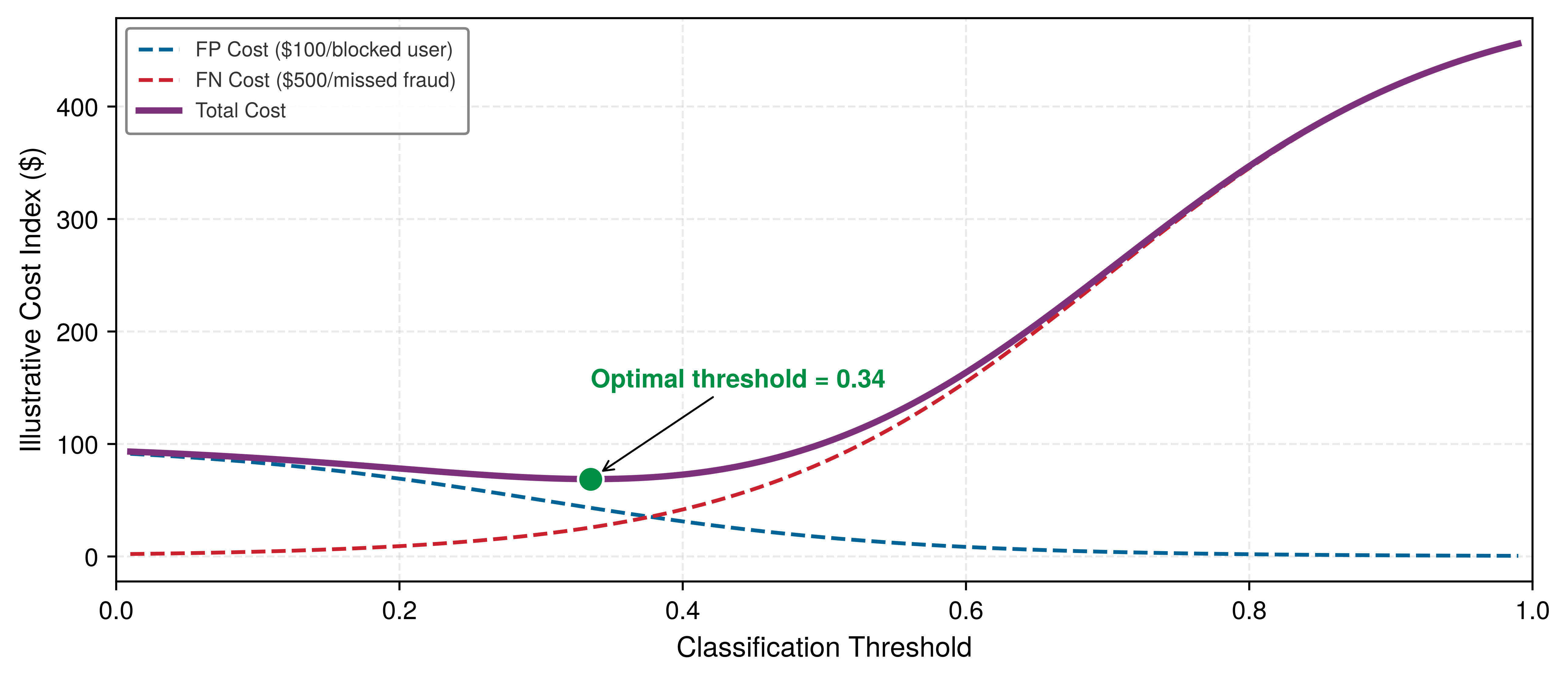
Incident communication presents another critical challenge. When a model degrades or requires rollback, stakeholders need the current evidence, affected populations, operational impact, mitigation, and remaining uncertainty. A fluctuation should not be dismissed as normal variation before it is tested, and drift is not merely planned maintenance when it is already harming outcomes. Regular performance reporting establishes the baseline that makes exceptional behavior easier to explain.

Resource justification requires translating technical requirements into business value. Rather than requesting “eight A100 GPUs for model training,” effective communication frames investments as “infrastructure to reduce experiment cycle time from weeks to days, enabling faster feature iteration.” Timeline estimation must account for realistic proportions: data preparation and deployment integration often dominate the schedule, while model development is only one part of the work.

Consider a fraud detection team implementing model improvements. When stakeholders request enhanced fraud capture, the team responds with a structured proposal: increasing the fraction of fraud dollars captured from 92 percent to 94 percent requires integrating external data sources, extending training duration by two weeks, and accepting 30 percent higher infrastructure costs, but would prevent an estimated $2 million in annual fraud losses while, under a separate 20 percent reduction assumption, reducing false-positive alerts by 50,000 per month.

Through disciplined stakeholder communication, MLOps practitioners maintain organizational support while establishing realistic expectations about system capabilities. This communication competency is as essential as technical expertise for sustaining successful ML operations.

ML test score

A release-readiness assessment needs a shared inventory of the debt patterns that can make a model unsafe to deploy even when its offline metrics look acceptable. Table 26 consolidates the patterns discussed throughout this chapter, providing the reference that the assessment rubric in table 27 builds on.

Table 26: Technical Debt Patterns: Machine learning systems accumulate distinct forms of technical debt from data dependencies, model interactions, and evolving operational contexts. Primary debt patterns, their causes, symptoms, and recommended mitigation strategies guide practitioners in recognizing and addressing these challenges systematically.

Debt Pattern	Primary Cause	Key Symptoms	Mitigation Strategies
Boundary Erosion	Tightly coupled components, unclear interfaces	Changes cascade unpredictably, CACE principle violations	Enforce modular interfaces, design for encapsulation
Correction Cascades	Sequential model dependencies, inherited assumptions	Upstream fixes break downstream systems, escalating revisions	Careful reuse vs. redesign trade-offs, clear versioning
Undeclared Consumers	Informal output sharing, untracked dependencies	Silent breakage from model updates, hidden feedback loops	Strict access controls, formal interface contracts, usage monitoring
Data Dependency Debt	Unstable or underutilized data inputs	Model failures from data changes, brittle feature pipelines	Data versioning, lineage tracking, leave-one-out analysis
Feedback Loops	Model outputs influence future training data	Self-reinforcing behavior, hidden performance degradation	Cohort-based monitoring, canary deployments, architectural isolation
Pipeline Debt	Ad hoc workflows, lack of standard interfaces	Fragile execution, duplication, maintenance burden	Modular design, workflow orchestration tools, shared libraries
Configuration Debt	Fragmented settings, poor versioning	Irreproducible results, silent failures, tuning opacity	Version control, validation, structured formats, automation
Prototype Debt	Rapid prototyping shortcuts, tight code-logic coupling	Inflexibility as systems scale, difficult team collaboration	Flexible foundations, intentional debt tracking, planned refactoring

With those debt patterns in one place, awareness alone is insufficient; teams need a systematic technical debt assessment rubric that transforms subjective “is this system ready?” conversations into quantifiable evaluations. The ML Test Score (Breck et al. 2017) provides a systematic rubric for evaluating production readiness across four categories: data tests, model tests, ML infrastructure tests, and monitoring tests. The paper defines 28 tests in total, seven per section, with partial or full credit for each test. Readiness is tracked by section rather than by a simple grand-total maturity band: a system with strong model tests but weak monitoring still carries production risk. Table 27 summarizes representative tests practitioners should implement:

Data section: Validates feature expectations, privacy controls, and whether each feature is beneficial relative to its operational cost.
Model section: Validates reviewed model specifications, hyperparameter discipline, staleness limits, and offline-online metric alignment.
Infrastructure section: Validates reproducible training, rollback, training-serving consistency, and deployment gates.
Monitoring section: Validates alerts for dependency changes, data invariants, skew, and model staleness.

Table 27: ML Test Score Checklist: Representative production-readiness tests from the ML Test Score rubric. The original rubric contains 28 tests grouped into four sections of seven tests each; section scores expose whether production risk comes from data validation, model validation, infrastructure, or monitoring rather than hiding the weakness in a single total. Based on Breck et al. (2017).

Category	Test	Implementation Example
Data Tests	Feature expectations are captured in schema	Great Expectations, TFX Data Validation
	All features are beneficial (no unused features)	Feature importance analysis, ablation studies
	No feature’s cost exceeds its benefit	Latency/accuracy trade-off analysis
	Data pipeline has appropriate privacy controls	PII detection, access logging
Model Tests	Model spec is reviewed and checked into version control	Git-tracked model configs
	Offline and online metrics are correlated	A/B test validation of offline improvements
	All hyperparameters are tuned	Automated HPO with tracked results
	Model staleness is measured and bounded	Performance decay monitoring
Infrastructure Tests	Training is reproducible	Fixed seeds, versioned data, locked dependencies
	Model can be rolled back to previous version	Model registry with versioning
	Training and serving code paths are tested for consistency	Feature store integration tests
	Model quality is validated before serving	Automated validation gates in CI/CD
Monitoring Tests	Dependency changes result in alerts	Data schema monitoring
	Data invariants hold in training and serving	Distribution comparison tests
	Training and serving features are not skewed	Training-serving skew detection
	Model staleness triggers retraining	Automated retraining pipelines

Quarterly audits against this rubric, prioritizing tests that address the most frequent incident types, reveal where operational investments will yield the highest reliability gains. Checking boxes is necessary but not sufficient. Production readiness requires understanding how practices integrate into a coherent system and how organizations evolve their capabilities over time.

Self-Check: Question

An engineering team needs to evaluate the live inference latency, resource consumption, and numerical output distribution of a new deep recommender against live production traffic without exposing users to potential prediction quality regressions. Which deployment pattern should they select?
1. Canary deployment, routing 5% of user-facing production traffic directly to the candidate model
2. Blue-green deployment, performing an immediate router-level cutover of 100% of user traffic
3. Shadow deployment, asynchronously duplicating live production traffic to the candidate model while returning only the incumbent model’s predictions to users
4. In-place deployment, updating the model weights directly on active production inference servers
A real-time inference service has a 100 ms P99 latency SLO partitioned as: Network RTT (15 ms), Feature retrieval (25 ms), Request parsing (5 ms), Model inference (45 ms), Postprocessing (5 ms), and Response serialization (5 ms). If the team applies weight quantization and kernel fusion to achieve a 2x speedup on model inference (reducing it from 45 ms to 22.5 ms), what is the new end-to-end P99 latency and overall system speedup?
1. 50.0 ms total latency, resulting in a 2.0x end-to-end speedup
2. 22.5 ms total latency, because inference was the sole target of optimization
3. 95.0 ms total latency, because non-inference stages expand to consume the budget
4. 77.5 ms total latency, resulting in approximately 1.3x end-to-end speedup
Explain why high-stakes production ML systems (such as medical diagnosis or loan underwriting) experience a ‘verification gap’ and describe how leading indicators mitigate this challenge.
A production ML monitoring pipeline processes streaming inference requests. Place the following monitoring checks in the logical order of the monitoring hierarchy, from earliest input validation to downstream business verification:

Model Output & Confidence Distribution Tracking: Log prediction distributions and softmax confidence scores.
Business KPI & Outcome Metric Evaluation: Correlate delayed ground-truth labels with conversion or default rates.
Infrastructure Health & Latency Telemetry: Measure CPU/GPU utilization, memory bandwidth, and P99 latency.
Input Schema & Null Value Validation: Verify column types, required fields, and physical range bounds.
Feature Distribution Drift Quantification: Compute PSI, KS statistics, or Wasserstein distance against baseline training distributions.

True or False: An inference server displaying 95% GPU compute utilization and 30% HBM memory bandwidth utilization should be optimized primarily by applying weight quantization to reduce memory bus traffic.
In statistical drift monitoring, a Population Stability Index value of $\text{PSI} >$ ____ is the standard operational threshold indicating a significant distribution shift that requires investigation.

See Answers →

Design and Maturity Framework

An organization deploying its initial ML model might rely on a hand-run Jupyter notebook, a scheduled cron job, and minimal monitoring. A mature enterprise runs thousands of models through automated pipelines with drift detection, canary deployments, and continuous validation. Both are doing “MLOps,” yet the gap between them spans orders of magnitude in reliability, cost efficiency, and engineering velocity. Deployment case studies show that practical challenges appear across the ML deployment workflow (Paleyes et al. 2022). This chapter uses operational maturity as a systems lens for that progression: organizations evolve from ad hoc experimentation toward fully automated operations, and understanding where a team stands on this continuum is as important as knowing the technical components themselves. Identifying what investments yield the highest returns at each stage guides resource allocation more effectively than adopting tools indiscriminately.

Paleyes, Andrei, Raoul-Gabriel Urma, and Neil D. Lawrence. 2022. “Challenges in Deploying Machine Learning: A Survey of Case Studies.” ACM Computing Surveys 55 (6): 1–29. https://doi.org/10.1145/3533378.

Maturity levels

The ML Test Score assesses individual practices. Operational maturity captures something broader: the systemic integration of those practices into a coherent whole. The key distinction is not which tools a team has adopted but how well infrastructure, automation, monitoring, governance, and collaboration work together across the ML lifecycle. Lifecycle tools such as MLflow address parts of that workflow (Zaharia et al. 2018), but maturity is the organizational ability to make the pieces work together. Although operational maturity exists on a continuum, distinguishing broad maturity levels helps illustrate how ML systems evolve from research prototypes to production-grade infrastructure.

Zaharia, Matei, Andrew Chen, Aaron Davidson, Ali Ghodsi, Sue Ann Hong, Andy Konwinski, Siddharth Murching, et al. 2018. “Accelerating the Machine Learning Lifecycle with MLflow.” IEEE Data Engineering Bulletin 41 (4): 39–45.

At the lowest level, ML workflows are ad hoc: experiments run manually, models train on local machines, and deployment involves hand-crafted scripts. As maturity increases, workflows become structured: teams adopt version control, automated training pipelines, and centralized model storage. At the highest levels, systems are fully integrated with infrastructure-as-code, continuous delivery pipelines, and automated monitoring that support large-scale deployment and rapid experimentation.

The distinguishing marker at each stage is not which tools a team adopts but how tightly infrastructure, automation, and monitoring integrate across the lifecycle. Table 28 shows that the leap from ad hoc to scalable is primarily an architectural shift from isolated scripts to a cohesive system.

Table 28: Maturity Progression: Machine learning operational practices evolve from manual, fragile workflows toward fully integrated, automated systems, impacting reproducibility and scalability. Key characteristics and outcomes at each maturity level emphasize architectural cohesion and lifecycle integration for building maintainable learning systems.

Maturity Level	System Characteristics	Typical Outcomes
Ad Hoc	Manual data processing, local training, no version control, unclear ownership	Fragile workflows, difficult to reproduce or debug
Repeatable	Automated training pipelines, basic CI/CD, centralized model storage, some monitoring	Improved reproducibility, limited scalability
Scalable	Fully automated workflows, integrated observability, infrastructure-as-code, governance	High reliability, rapid iteration, production-grade ML

Consider how a fraud detection system evolves across these maturity levels:

Ad hoc: A data scientist trains a model in a Jupyter notebook, exports it as a pickle file, and hands it to an engineer who deploys it to a single server. When accuracy drops, the data scientist retrains manually by running the notebook again with fresh data. Debugging requires the original data scientist because no one else understands the preprocessing steps.
Repeatable: The training script is version-controlled, with a scheduled Jenkins job that retrains monthly. Features are computed in a SQL script that engineering maintains separately. The model is deployed via container, with basic accuracy monitoring. When the feature SQL changes, the data scientist must manually verify the model still works.
Scalable: Training and serving use the same feature store, reducing skew. A CI/CD pipeline investigates drift when PSI exceeds 0.2, retrains when evidence supports it, validates the new model against the baseline, and deploys via canary release. Monitoring tracks per-merchant accuracy, triggering investigation when specific segments degrade. The entire lineage from raw data to production prediction is auditable.

The investment required to move between levels is substantial and often spans months of engineering effort, but the reduction in incident frequency and debugging time can justify the cost for production-critical systems.

These maturity levels provide a systems lens through which to evaluate ML operations, not in terms of specific tools adopted, but in how reliably and cohesively a system supports the full machine learning lifecycle. Understanding this progression prepares practitioners to identify design bottlenecks and prioritize investments that support long-term system sustainability.

System design implications

Maturity levels describe organizational stages; system design implications describe the architectural consequences. At each level, the system architecture evolves in response to new expectations around modularity, automation, monitoring, and fault tolerance.

In low-maturity environments, ML systems are monolithic: data processing logic embedded in model code, configurations managed informally, and deployments handled through ad hoc scripts. These architectures enable rapid experimentation but lack the separation of concerns needed for maintainability or safe iteration. As maturity increases, modular abstractions emerge: feature engineering decouples from model logic, pipelines become declarative, and system boundaries are enforced through APIs. At high maturity, ML systems exhibit properties of production-grade software (stateless services, contract-driven interfaces, environment isolation, and observable execution) where data, models, and infrastructure co-evolve through closed feedback loops.

Figure 10 captures this architectural reality as an iceberg. What stakeholders see (uptime, the visible tip) represents only a fraction of what must work correctly beneath the surface. The hidden mass below the waterline shows the threats that can sink a system even when it appears healthy: data drift, concept drift, broken pipelines, schema changes, model bias, and underperforming segments. Operational maturity must address all three domains (data health, model health, service health) simultaneously.

\scalebox{0.65}{%
\begin{tikzpicture}[line join=round,font=\sffamily\small]
\tikzset{Line/.style={line width=1.5pt,BlueD},
 mysnake/.style={postaction={line width=2.5pt,BlueD,draw,decorate,
 decoration={snake,amplitude=1.8pt,segment length=18pt}}},
pics/flag/.style = {
        code = {
        \pgfkeys{/channel/.cd, #1}
\begin{scope}[local bounding box=FLAG,scale=\scalefac, every node/.append style={transform shape}]
\draw[draw=\drawchannelcolor,fill=\channelcolor](0.15,1.07)to[out=30,in=220](1.51,1.07)to(1.51,2.02)
           to[out=210,in=40](0.15,2.04)--cycle;
\draw[draw=none,fill=\channelcolor](0.05,0)rectangle (-0.05,2.1);
\fill[fill=\channelcolor](0,2.1)circle(3pt);
\end{scope}
     }
  }
}
\pgfkeys{
  /channel/.cd,
  channelcolor/.store in=\channelcolor,
  drawchannelcolor/.store in=\drawchannelcolor,
  scalefac/.store in=\scalefac,
  Linewidth/.store in=\Linewidth,
  picname/.store in=\picname,
  channelcolor=BrownLine,
  drawchannelcolor=BrownLine,
  scalefac=1,
  Linewidth=1.6pt,
  picname=C
}
\colorlet{BlueD}{GreenD}

\begin{scope}[local bounding box=FLAG1,shift={($(0,0)+(0,0)$)},
scale=1, every node/.append style={transform shape}]
\pic[shift={(0,0)}] at  (0,0){flag={scalefac=0.45,picname=1,drawchannelcolor=none,channelcolor=GreenD, Linewidth=1.0pt}};
 \end{scope}
%
\path[top color=GreenD!60,bottom color=GreenD](-1.69,-1.69)--(-2,-2)--(-2.5,-2.06)--(-3.1,-3.0)--(-4,-3.84)--(-3.72,-4.33) --(-3.95,-4.5)
 --(-2.85,-5.92)--(-3,-6.059)--(-1.84,-7.341)-- (1.9,-7.341)--(3.58,-5.45)--(3.35,-4.56)--(3.91,-3.5)--(3.5,-3.18)
 --(2.82,-2.11)--(2.25,-2.05)--(1.85,-1.69)--cycle;
  \draw[Line](-1.13,-1.14)--(-2,-2)--(-2.5,-2.06)--(-3.1,-3.0)--(-4,-3.84)--(-3.72,-4.33) --(-3.95,-4.5)
 --(-2.85,-5.92)--(-3,-6.059)--(-1.84,-7.341)-- (1.9,-7.341)--(3.58,-5.45)--(3.35,-4.56)--(3.91,-3.5)--(3.5,-3.18)
 --(2.82,-2.11)--(2.25,-2.05)--(1.2,-1.14);
 \node[draw=none,rectangle,minimum width=140mm,inner sep=0pt, minimum height=2mm](TA)at(0,-1.7){};
\path[mysnake](TA.west)--(TA.east);
\draw[Line](0,0)--(-0.6,-0.63);
\draw[Line](-0.45,-0.65)--(-0.84,-0.60)--(-1.26,-1.41);
\draw[Line](0,0)--(0.57,-0.55);
 \draw[Line](0.45,-0.61)--(0.84,-0.37)--(1.38,-1.51);
 %
\node[BlueD]at(0,-1.2){UPTIME};
\node[white]at(1.2,-2.4){MODEL ACCURACY};
\node[white]at(-1.34,-2.75){DATA DRIFT};
\node[white]at(2.1,-3.35){CONCEPT DRIFT};
\node[white]at(-1.85,-3.75){BROKEN PIPELINES};
\node[white]at(-0.05,-4.5){SCHEMA CHANGE};
\node[white]at(1.8,-5.2){MODEL BIAS};
\node[white]at(-1.5,-5.4){DATA OUTAGE};
\node[white,align=center]at(0.15,-6.4){UNDERPERFORMING\\ SEGMENTS};
%
\node[BlueD]at(-5,-2.65){Data health};
\node[BlueD]at(5,-2.6){Model health};
\node[BlueD]at(2.8,0.1){Service health};
\end{tikzpicture}}

Figure 10: Uptime Dependency Stack: The waterline separates visible service uptime from data- and model-health failures that can remain hidden while the service stays available; the surrounding labels organize the monitoring surface into data, model, and service health.

The three threat categories in the iceberg map to distinct failure mechanisms. Data health threats (drift, staleness, and schema changes) erode the statistical assumptions a model was trained on, often without any change to the model itself. Model health threats (accuracy degradation, bias amplification, and feedback loops) compound silently because the model continues to produce outputs that appear well-formed even as their quality decays. Service health threats (configuration sprawl, pipeline fragmentation, and stale dependencies) undermine reproducibility and recoverability. Several of these failures can leave the service available, which is why availability monitoring alone cannot cover the full operational state.

Design patterns and anti-patterns

The most sophisticated infrastructure fails without the organizational patterns to operate it effectively. A feature store cannot prevent training-serving skew if no one owns the feature definitions; automated monitoring cannot catch drift if alerts route to the wrong team. As ML systems grow in complexity, organizational patterns must evolve to match.

In mature environments, organizational design emphasizes clear ownership and interface discipline. Platform teams may take responsibility for shared infrastructure and CI/CD pipelines while domain teams focus on model development and business alignment. Interfaces between teams (feature definitions, data schemas, and deployment targets) are well-defined and versioned.

One effective pattern is a centralized MLOps team providing shared services to multiple model development groups. Such structures promote consistency and reduce duplicated effort. Alternatively, some organizations adopt a federated model, embedding MLOps engineers within product teams while maintaining a central architectural function for system-wide integration.

Anti-patterns emerge when responsibilities are fragmented. The tool-first approach (adopting infrastructure tools without first defining processes and roles) results in fragile pipelines and unclear handoffs. Siloed experimentation, where data scientists operate in isolation from production engineers, leads to models that are difficult to deploy or retrain effectively.

Organizational drift presents another challenge. As teams scale, undocumented workflows become entrenched and coordination costs increase. Organizational maturity must co-evolve with system complexity through communication patterns, role definitions, and accountability structures that reinforce modularity, automation, and observability.

These organizational patterns must be supported by technical architectures handling the reliability challenges of ML systems. MLOps inherits distributed systems challenges but adds complications through learning components requiring adaptations for probabilistic behavior. Conventional services can also return incorrect results without crashing; ML systems add statistical and data-dependent failure modes that availability checks cannot detect.

Circuit breaker patterns must account for model-specific failure modes, where prediction accuracy degradation requires different thresholds than service availability failures. Bulkhead patterns²⁹ become critical when isolating experimental model versions from production traffic. These patterns require resource partitioning strategies that prevent resource exhaustion in one model from affecting others. Ordinary model prediction errors are semantic failures, not Byzantine faults; Byzantine fault tolerance³⁰ provides only a limited analogy for arbitrary component failures.

²⁹ Bulkhead pattern: This pattern partitions system resources to contain failures within isolated zones. For isolating experimental models, a bulkhead dedicates a fixed compute and memory budget to the new version. This resource partition ensures that a catastrophic failure in the experiment, such as a memory leak, cannot exhaust all available resources and cause a system-wide production outage.

³⁰ Byzantine fault tolerance: The classic Byzantine model concerns nodes that may behave arbitrarily or send conflicting messages. In the synchronous unauthenticated, or oral-messages, setting, tolerating $f$ Byzantine faults requires at least $3f+1$ participants (Lamport et al. 1982). ML ensembles are only an analogy because prediction errors can be correlated, and agreement does not establish semantic correctness.

Lamport, Leslie, Robert Shostak, and Marshall Pease. 1982. “The Byzantine Generals Problem.” ACM Transactions on Programming Languages and Systems 4 (3): 382–401. https://doi.org/10.1145/357172.357176.

Consensus algorithms establish agreement among nodes; they cannot determine whether a model prediction is correct when ground truth is delayed or unavailable. These reliability patterns nevertheless help distinguish robust MLOps implementations from fragile ones when their guarantees are applied within scope.

Contextualizing MLOps

Best practices are rarely deployed in pristine environments. Every ML system operates within a specific context that shapes how practices are implemented: physical constraints (edge compute, power budgets), regulatory requirements (healthcare, finance), or organizational realities (team size, skill distribution). A standard CI/CD pipeline may be infeasible without direct host access; monitoring may require indirect signals or on-device anomaly detection; data collection may be limited by privacy regulations. These adaptations are expressions of maturity under constraint, not departures from the principles.

At the highest levels of operational maturity, the single-model practices established here become building blocks for larger organizational capabilities. Organizations operating many ML nodes simultaneously often consolidate into platform architectures that provide shared infrastructure, centralized governance, and economies of scale. The transition from individual ML nodes to platform-scale infrastructure introduces qualitatively different challenges (cross-model resource allocation, system-level observability, fault tolerance for interdependent AI systems) that extend beyond this chapter’s single-model scope. Sound ML node practices are prerequisites for platform success because gaps in single-model monitoring, testing, or deployment multiply across the model portfolio.

MLOps investment economics

The operational benefits of MLOps become persuasive only when the investment matches the model’s production value. For a single ML node, the decision is whether deployment speed, incident reduction, and monitoring coverage justify the operational spend; for a portfolio, the same economics compound into platform investment.

Single-model MLOps investment

For a single production ML system, the first threshold is the annual cost of making the node observable, deployable, and recoverable. Table 29 summarizes the main cost categories:

Table 29: Single-Model MLOps Investment: Illustrative planning inputs for operationalizing one production ML system. Open-source tooling (MLflow, Feast) can reduce software costs; cloud-managed services trade higher unit costs for reduced engineering overhead.

Component	Illustrative Assumption	Justification
CI/CD pipeline setup	$10–30K one-time	Reduces deployment time from days to hours
Monitoring and alerting	$2–10K/year	Catches degradation before user impact
Feature store (basic)	$5–20K/year	Reduces one source of training-serving skew
Model registry	$0–5K/year	Enables rollback, audit trails
Engineering time	1–2 FTE-months setup	Initial automation and integration

Single-model ROI calculation

The return threshold then depends on model criticality: a revenue-facing model can justify more operational spend because avoided incidents and deployment-time savings have measurable value. Equation 16 formalizes that single-node calculation: \[\text{Annual Benefit/Cost} = \frac{\text{Incidents Avoided} \times \text{Avg Incident Cost} + \text{Time Savings} \times \text{Hourly Cost}}{\text{Annual MLOps Investment}} \tag{16}\] where Incidents Avoided is the count of production failures the tooling prevents per year and Avg Incident Cost is the loss per failure, so their product is the value of avoided incidents; Time Savings is the engineer-hours that automation reclaims per year and Hourly Cost is the loaded labor rate, so their product is the value of recovered labor; the denominator is the annual cost of the tooling itself. The ratio expresses every dollar of investment in dollars returned.

For a model generating $1M annual revenue with:

4 incidents/year avoided (at $25K each) = $100K saved
20 hours/month deployment time saved (at $150/hr) = $36K saved
MLOps investment of $30K/year

\[ \text{Benefit/Cost} = \frac{\$100K + \$36K}{\$30K} = 4.53× \]

When to invest more

The 4.53× benefit-cost ratio means the investment is not justified by tooling elegance; it is justified because the model is expensive enough that preventing incidents and shortening deployments outweigh the annual platform spend. The returns from single-model MLOps practices compound when teams add additional models. The transition from operating several independent ML nodes to building a centralized platform involves different economics entirely, including shared infrastructure amortization, platform team overhead, and cross-model coordination costs.

For single-model operations, invest in MLOps in proportion to model criticality. A model driving $10M in annual revenue justifies more operational rigor than an internal analytics model. Monitoring, lineage, and repeatable deployment are often the first investments. Add a feature store when shared feature definitions and online-offline parity become material problems, and automate retraining only when evidence supports the trigger and the validation loop can contain a bad update.

The preceding technical infrastructure and economic framework provide the foundation; the case studies in section 1.7 demonstrate how these elements combine in production systems. Each case demonstrates specific implementations of the five foundational principles, identifying where reproducibility appears, how observable degradation is achieved, and what triggers automation.

Self-Check: Question

What fundamental reliability concept is illustrated by the ‘Uptime Iceberg’ metaphor in production machine learning systems?
1. Traditional service availability (uptime and low latency) is only the visible tip; hidden failures like feature drift, concept drift, schema corruption, and subpopulation degradation lurk beneath the surface
2. Distributed feature retrieval latency over wide-area networks always exceeds local GPU inference execution time
3. Data center cooling overhead exceeds the total electrical power consumed by GPU inference accelerators
4. Deep neural network weight storage in DRAM requires larger memory allocations than raw training dataset storage
An organization with limited engineering resources is deploying its first production ML model. Based on the chapter’s investment economics framework, which staging sequence provides the most cost-effective path to reliability?
1. Construct an enterprise-wide multi-region distributed feature store and autonomous retraining cluster before deploying the initial model
2. Invest first in statistical monitoring and basic CI/CD deployment pipelines, then add centralized feature stores and automated retraining as model scale and drift warrant
3. Procure an all-in-one commercial MLOps platform suite to eliminate cross-functional on-call rotations
4. Defer all monitoring and automation investments until multiple major production outages have occurred
Describe the organizational anti-pattern of ‘tossing models over the wall’ between data scientists and software engineers, and explain how a cross-functional or federated MLOps structure resolves it.
An engineering team is assessing the operational maturity of an ML deployment. Place the three operational maturity stages in order from least mature to most mature:

Repeatable: Version-controlled training scripts, scheduled batch retraining jobs, centralized model registry, and basic performance monitoring.
Scalable: Unified feature store enforcing training-serving parity, closed-loop drift detection with automated canary validation, and infrastructure-as-code.
Ad Hoc: Hand-crafted Jupyter notebooks, local training on developer machines, manual pickle file deployment, and absence of formal versioning.

See Answers →

Case Studies

A battery-powered sleep-tracking ring and AI/ML-based medical software governed by FDA lifecycle expectations (U.S. Food and Drug Administration 2025) face different operational constraints. The principles, patterns, and infrastructure examined throughout this chapter converge differently depending on the deployment context. An Oura-inspired edge design shows how pipeline debt and configuration management challenge resource-constrained environments; ClinAIOps shows how feedback loops and governance requirements reshape healthcare operations. The Oura lifecycle in section 1.7.1 is hypothetical; the cited study supports offline data and model evaluation, not claims about Oura’s production OTA or MLOps implementation. The comparison starts with the shared principles, because the domains differ most in how those principles are implemented.

U.S. Food and Drug Administration. 2025. Marketing Submission Recommendations for a Predetermined Change Control Plan for Artificial Intelligence-Enabled Device Software Functions. Guidance for Industry and Food and Drug Administration Staff. U.S. Department of Health; Human Services.

Table 30 lays out how the two environments could implement the five foundational MLOps principles. Domain constraints (edge hardware, clinical regulation) reshape how each principle is realized without changing which principles matter. In the Oura-inspired design, polysomnography (PSG) refers to the clinical sleep-study measurements used as reference labels.

The principles stay stable, but their implementation changes with the deployment regime. Edge systems spend the automation budget on battery, telemetry, and constrained updates; clinical systems spend it on auditability, validation gates, and accountable human control. The two case studies that follow trace how each environment earns those entries.

Table 30: MLOps Principles by Case Study: Side-by-side mapping of the five foundational MLOps principles to a hypothetical Oura-inspired edge design and the ClinAIOps framework, showing how domain constraints reshape implementation without changing which principles apply.

Principle	Oura-inspired edge design	ClinAIOps
Reproducibility	Versioned synchronized wearable and PSG datasets	Audit trails, decision provenance
Separation of concerns	Independent data, training, and serving layers with edge-specific deployment pipeline	Distinct clinical validation and deployment stages with regulatory compliance isolation
Consistency	PSG-aligned preprocessing across training and on-device inference	Standardized clinical data pipelines ensuring training-serving parity
Observable degradation	On-device anomaly detection, limited telemetry	Cohort-specific monitoring, outcome tracking
Cost-aware automation	Battery-aware retraining triggers, CI/CD for edge balancing accuracy and resource cost	Automated model updates with human-in-the-loop gates balancing update cost and patient risk

Oura-inspired edge design

The Oura Ring provides the offline evidence behind this Oura-inspired MLOps design. The published work supports the clinical data collection and sleep-stage evaluation described later (Altini and Kinnunen 2021), while the versioning, telemetry, over-the-air deployment, and iterative refinement cycle are a hypothetical architecture rather than a reported account of Oura’s production lifecycle. The constraints imposed by a battery-powered ring with limited compute make every MLOps decision visible in a way that cloud-scale systems can obscure.

Context and motivation

The Oura Ring is a consumer-grade wearable monitoring sleep, activity, and physiological recovery through embedded sensing and computation. By measuring motion, heart rate, and body temperature, the device estimates sleep stages and delivers personalized feedback. An Oura-inspired design may place selected preprocessing and inference on the device while other processing occurs on a phone or in the cloud.

The central objective was improving sleep stage classification accuracy to align more closely with polysomnography (PSG),³¹ the clinical gold standard. Initial evaluations showed 57 percent four-stage sleep classification accuracy for an accelerometer-only model, compared with 79 percent for models that included autonomic nervous system and circadian features. Published human PSG inter-scorer reliability is about 82 percent to 83 percent, framing the remaining gap between wearable inference and expert clinical scoring. The 22 percentage-point gain closes roughly 84.6–88 percent of the baseline-to-human-agreement gap, although inter-scorer agreement is not a ceiling on accuracy against a fixed or adjudicated reference. This discrepancy prompted an effort to re-evaluate data collection, preprocessing, and model development workflows.

³¹ Polysomnography (PSG): A multi-parameter sleep study that provides the clinical ground truth data for this classification task. This ‘truth’ is inherently noisy; expert human scorers interpreting the same PSG recordings agree with each other at about 82 percent–83 percent reliability (Altini and Kinnunen 2021). Inter-scorer agreement indicates label uncertainty but does not impose an accuracy ceiling against a fixed or adjudicated reference.

Altini, Marco, and Hannu Kinnunen. 2021. “The Promise of Sleep: A Multi-Sensor Approach for Accurate Sleep Stage Detection Using the Oura Ring.” Sensors 21 (13): 4302. https://doi.org/10.3390/s21134302.

To overcome performance limitations, the Oura team constructed a diverse dataset grounded in clinical standards through a study involving 106 participants from three continents (Altini and Kinnunen 2021). Each participant wore the Oura Ring while simultaneously undergoing PSG, yielding 440 nights of data and 3,444 hours of time-synchronized recordings that aligned wearable sensor data with validated sleep annotations. The scale and diversity of the collection captured physiological variation as well as environmental and behavioral factors critical for generalizing across a real-world user base.

The study consolidated synchronized accelerometer, temperature, heart-rate, heart-rate-variability, and PSG data from research Oura rings, then resolved temporal alignment and preprocessing requirements for downstream model development. A hypothetical production workflow would add robust versioning and lineage tracking to avoid unstable dependencies that commonly plague embedded ML systems.

With high-quality data in place, the study’s next question was whether extra sensing improved sleep-stage classification. The researchers evaluated four offline configurations that incrementally added temperature, heart-rate variability, and circadian features to an accelerometer-only baseline. Through 5-fold cross-validation against PSG annotations, the enhanced models achieved 79 percent four-stage classification accuracy, an improvement from the 57 percent accelerometer-only baseline (Altini and Kinnunen 2021). These offline gains motivate the hypothetical production design, but its reproducible training, versioning, conversion validation, and energy controls are inferred requirements rather than results reported by the study.

³² Over-the-air (OTA) updates: The mechanism used to deploy optimized models to devices already in the field, bypassing the need for physical access. The small footprint from quantization and pruning matters because constrained edge networks may need to transmit only changed model artifacts rather than complete application bundles. This process makes consistency a critical concern; a failed update can corrupt the on-device model, breaking the ML pipeline until a future connectivity window allows for a fix.

Following validation, deployment shifted the problem from model quality to update safety. An Oura-like edge deployment must decide which parts of the model run continuously on-device, which richer signals can be used under looser memory and battery budgets, and how model updates reach devices already in the field. To keep that split maintainable, the operational toolchain needs reproducible model conversion, versioned artifacts, and authenticated OTA³² update procedures that preserve consistency across devices in the field.

The operational lesson is that edge MLOps is not governed by accuracy alone; it is governed by accuracy under battery, privacy, telemetry, and weak ground truth constraints. Consider the DS-CNN (Tiny Constraint) archetype from table 4, where monitoring relies on operational metrics such as duty cycle and false positive rate rather than continuous ground-truth labels, and an illustrative quarterly cadence governs OTA updates. Operationalizing the transition from 57 percent accelerometer-only accuracy to 79 percent multi-sensor accuracy would require systematic configuration management across data collection, feature sets, model architectures, and deployment targets.

Those constraints explain how the foundational principles appear without repeating them as a checklist. Versioned wearable and PSG datasets make each model traceable to the evidence used to train it. Modular tiered architectures keep data collection, model training, and on-device serving separate enough that quantization, pruning, and fallback policies can change without destabilizing the whole pipeline. PSG-aligned preprocessing preserves consistency between training and on-device inference, while privacy-preserving telemetry makes degradation observable through duty cycle, battery impact, inference failures, confidence, anomaly rates, and periodic labeled studies. OTA deployment then becomes the cost-aware automation boundary: updates must justify their accuracy gain against battery impact, validation burden, and the risk of changing software on a device worn continuously by users.

This case exemplifies how MLOps principles adapt to domain-specific constraints. When machine learning moves into clinical applications, additional complexity emerges, requiring frameworks that address regulatory compliance, patient safety, and clinical decision-making.

ClinAIOps case study

Healthcare ML deployment presents challenges extending beyond resource constraints. General-purpose MLOps frameworks require additional controls in domains with extensive human oversight, domain-specific evaluation, and ethical governance. Continuous therapeutic monitoring (CTM)³³ exemplifies a domain where MLOps must evolve to meet clinical integration demands.

³³ Continuous therapeutic monitoring (CTM): Healthcare approach using wearable sensors for real-time physiological data collection and personalized treatment adjustments. CTM forces MLOps to confront constraints absent in typical deployments: feedback loops must include human-in-the-loop approval for safety-critical decisions, retraining requires clinician-validated labels rather than implicit signals, and model updates must satisfy regulatory compliance before deployment. These constraints reshape every MLOps principle, making CTM a stress test for operational maturity.

CTM uses wearable sensors to collect real-time physiological and behavioral data from patients. AI systems must be integrated into clinical workflows, aligned with regulatory requirements, and designed to augment rather than replace human decision-making. General-purpose MLOps practices provide technical lifecycle controls, but they do not by themselves prescribe clinical responsibility, evidence standards, or decision authority.

ClinAIOps (Chen et al. 2023), a framework for operationalizing AI in clinical environments, shows how MLOps principles must evolve for regulatory and human-centered requirements. Unlike conventional MLOps, ClinAIOps directly addresses feedback loop challenges by designing them into the system architecture. The framework’s structured coordination between patients, clinicians, and AI developers represents practical implementation of governance and collaboration principles.

Clinical environments therefore extend the ordinary operational problem. Healthcare requires coordination among diverse human actors, clinical decisions depend on personalized care and shared accountability, and health data is subject to strict privacy and governance requirements. ClinAIOps presents a framework that balances technical rigor with clinical utility and operational reliability with ethical responsibility.

Feedback loops

Three interlocking feedback loops enable safe, adaptive integration of machine learning into clinical practice. Figure 11 maps these loops as a circular flow among three stakeholders. Patients contribute continuous monitoring data from wearable sensors and receive bounded AI-assisted guidance. Clinicians receive AI-generated summaries, alerts, and recommendations, then apply clinical judgment by setting therapy regimens and approval limits. AI developers receive continuous feedback from patients and clinicians, using real-world performance and workflow signals to improve models and deployment processes. The outer loop connecting all three stakeholders represents the full governance cycle.

\scalebox{0.85}{%
\begin{tikzpicture}[line join=round,font=\small\sffamily]
%radius
\def\ra{53mm}
\newcommand{\gear}[6]{%
  (0:#2)
  \foreach \i [evaluate=\i as \n using {(\i-1)*360/#1}] in {1,...,#1}{%
    arc (\n:\n+#4:#2) {[rounded corners=1.5pt] -- (\n+#4+#5:#3)
    arc (\n+#4+#5:\n+360/#1-#5:#3)} --  (\n+360/#1:#2)
  }%
  (0,0) circle[radius=#6];
  \scoped[on background layer]
}

\tikzset{
  man/.pic={
  \pgfkeys{/man/.cd, #1}
     % tie
    \draw[draw=\tiecolor,fill=\tiecolor] (0.0,-1.1)--(0.16,-0.87)--(0.09,-0.46)--(0.13,-0.37)--(0.0,-0.28)--(-0.13,-0.37)--(-0.09,-0.46)--(-0.16,-0.87)--cycle;
    % ears
    \draw[fill=black,draw=none] (0.74,0.95) to[out=20,in=80](0.86,0.80) to[out=250,in=330](0.65,0.65) to[out=70,in=260] cycle;
    \draw[fill=black,draw=none] (-0.76,0.96) to[out=170,in=110](-0.85,0.80) to[out=290,in=190](-0.65,0.65) to[out=110,in=290] cycle;

    % head
    \draw[fill=black,draw=none] (0,0) to[out=180,in=290](-0.72,0.84) to[out=110,in=190](-0.56,1.67)
               to[out=70,in=110](0.68,1.58) to[out=320,in=80](0.72,0.84) to[out=250,in=0] cycle;
    % face
    \draw[fill=white,draw=none] (0,0.11) to[out=175,in=290](-0.53,0.65) to[out=110,in=265](-0.61,1.22)
                      to[out=80,in=235](-0.50,1.45) to[out=340,in=215](0.50,1.47)
                      to[out=310,in=85](0.60,0.92) to[out=260,in=2] cycle;
    \draw[fill=black,draw=none] (-0.50,1.45) to[out=315,in=195](0.40,1.25) to[out=340,in=10](0.37,1.32)
                      to[out=190,in=310](-0.40,1.49) -- cycle;
    % neck
    \draw[line width=1.5pt] (-0.62,-0.2) to[out=50,in=290] (-0.5,0.42);
    \draw[line width=1.5pt] (0.62,-0.2) to[out=130,in=250] (0.5,0.42);
    % body
    \draw[draw=\bodycolor,fill=\bodycolor] (0.0,-1.0) to[out=150,in=290](-0.48,-0.14) to[out=200,in=50](-1.28,-0.44)
                   to[out=240,in=80](-1.55,-2.06) -- (1.55,-2.06)
                   to[out=100,in=300](1.28,-0.44) to[out=130,in=340](0.49,-0.14)
                   to[out=245,in=30] cycle;
    % right stet
    \draw[line width=2pt,\stetcolor] (0.8,-0.21) to[bend left=7](0.78,-0.64)
         to[out=350,in=80](0.98,-1.35) to[out=250,in=330](0.72,-1.60);
    \draw[line width=2pt,\stetcolor] (0.43,-1.53) to[out=180,in=240](0.3,-1.15)
         to[out=60,in=170](0.78,-0.64);
    % left stet
    \draw[line width=2pt,\stetcolor] (-0.75,-0.21) to[bend right=20](-0.65,-1.45);
    \node[fill=\stetcolor,circle,minimum size=5pt] at (-0.65,-1.45) {};
    % eyes
    \node[circle,fill=black,inner sep=2pt] at (0.28,0.94) {};
    \node[circle,fill=black,inner sep=2pt] at (-0.28,0.94) {};
     % mouth
    \draw[line width=1.0pt] (-0.25,0.5) to[bend right=40](0.25,0.5);
  },
}
\pgfkeys{
  /man/.cd,
  tiecolor/.store in=\tiecolor,
  bodycolor/.store in=\bodycolor,
  stetcolor/.store in=\stetcolor,
  tiecolor=red,      % default tie color
  bodycolor=blue!30, % default body color
  stetcolor=green    % default stet color
}

\begin{scope}[local bounding box=PAC,
shift={($(90: 0.5*\ra)+(0,0.3)$)},
scale=0.5, every node/.append style={transform shape}]
\pic[scale=1] {man={tiecolor=red!50!yellow, bodycolor=green!50!blue,stetcolor=green!50!blue}};
\end{scope}

\begin{scope}[local bounding box=DOC,
shift={($(210: 0.5*\ra)+(-0.4,0.1)$)},
scale=0.5, every node/.append style={transform shape}]
\pic at (0,0) {man={tiecolor=red, bodycolor=VioletLine2,stetcolor=yellow}};
\end{scope}

\begin{scope}[local bounding box=GEAR,
shift={($(330: 0.5*\ra)+(0.5,0)$)},
scale=0.7, every node/.append style={transform shape}]
\fill[draw=none,fill=green!50!red,even odd rule] \gear{14}{1.2}{1.4}{10}{2}{0.9}coordinate(2GER1);
\end{scope}

\definecolor{CPU}{RGB}{0,120,176}
\begin{scope}[local bounding box = CPU,scale=0.3, every node/.append style={transform shape},
shift={($(GEAR)+(0,0)$)}]
\node[fill=CPU,minimum width=66, minimum height=66,
            rounded corners=2,outer sep=2pt] (C1) {};
\node[fill=white,minimum width=54, minimum height=54] (C2) {};
\node[fill=CPU!40,minimum width=44, minimum height=44,align=center,inner sep=0pt] (C3) {\huge AI};

\foreach \x/\y in {0.11/1,0.26/2,0.41/3,0.56/4,0.71/5,0.85/6}{
\node[fill=CPU,minimum width=3, minimum height=12,
           inner sep=0pt,anchor=south](GO\y)at($(C1.north west)!\x!(C1.north east)$){};
}
\foreach \x/\y in {0.11/1,0.26/2,0.41/3,0.56/4,0.71/5,0.85/6}{
\node[fill=CPU,minimum width=3, minimum height=12,
           inner sep=0pt,anchor=north](DO\y)at($(C1.south west)!\x!(C1.south east)$){};
}
\foreach \x/\y in {0.11/1,0.26/2,0.41/3,0.56/4,0.71/5,0.85/6}{
\node[fill=CPU,minimum width=12, minimum height=3,
           inner sep=0pt,anchor=east](LE\y)at($(C1.north west)!\x!(C1.south west)$){};
}
\foreach \x/\y in {0.11/1,0.26/2,0.41/3,0.56/4,0.71/5,0.85/6}{
\node[fill=CPU,minimum width=12, minimum height=3,
           inner sep=0pt,anchor=west](DE\y)at($(C1.north east)!\x!(C1.south east)$){};
}
\end{scope}
\draw[{Triangle[width=12pt,length=8pt]}-, line width=5pt,violet!80] (355:0.5*\ra)
                arc[radius=0.5*\ra, start angle=-5, end angle= 67]node[left,pos=0.3,
                align=center,font=\footnotesize\sffamily,text=black]{Continuous \\monitoring data\\ and health report};
\draw[{Triangle[width=12pt,length=8pt]}-, line width=5pt,CPU] (110:0.5*\ra)
arc[radius=0.5*\ra, start angle=110, end angle= 181]node[right=0.3,pos=0.66,
                align=center,font=\footnotesize\sffamily,text=black]{Therapy\\ regimen};
\draw[{Triangle[width=12pt,length=8pt]}-, line width=5pt,red!70] (233:0.5*\ra)
arc[radius=0.5*\ra, start angle=233, end angle= 311]node[above=0.4,pos=0.5,
                align=center,font=\footnotesize\sffamily,text=black]{
Alerts for therapy\\ modifications and\\ monitor summaries};
%%bigger circle
%radius
\def\ra{68mm}
\draw[-{Triangle[width=12pt,length=8pt]}, line width=5pt,violet!40] (353:0.5*\ra)
                arc[radius=0.5*\ra, start angle=-7, end angle= 77]node[right=0.21,pos=0.5,
                align=center,font=\footnotesize\sffamily,text=black]{Alerts for\\ clinician-approved\\
                therapy updates};
\draw[-{Triangle[width=12pt,length=8pt]}, line width=5pt,CPU!40] (105:0.5*\ra)
arc[radius=0.5*\ra, start angle=105, end angle= 185]node[left=0.2,pos=0.5,
                align=center,font=\footnotesize\sffamily,text=black]{Health challenges\\ and goals};
\draw[-{Triangle[width=12pt,length=8pt]}, line width=5pt,red!40] (232:0.5*\ra)
arc[radius=0.5*\ra, start angle=232, end angle= 305]node[below=0.11,pos=0.5,
                align=center,font=\footnotesize\sffamily,text=black]{
Limits and approvals \\of therapy regimens};
%
\node[below=0.1of PAC]{\textbf{Patient}};
\node[below=0.1of DOC]{\textbf{Clinician}};
\node[below=0.48of CPU]{\textbf{AI developer}};
\end{tikzpicture}}

Figure 11: ClinAIOps Feedback Loops: The cyclical framework coordinates patients, clinicians, and AI developers to support continuous model improvement and safe clinical integration. Patients and clinicians use AI outputs in care workflows, while AI developers receive feedback from both groups to refine models and operations. Source: (Chen et al. 2023).

Each feedback loop plays a distinct yet interconnected role; together, these loops enable adaptive personalization, maintain clinician control, and promote continuous model improvement based on real-world feedback:

The patient treatment loop captures real-time physiological data and uses bounded AI outputs to support patient self-management.
The clinician oversight loop ensures AI-assisted recommendations are reviewed, limited, and refined under professional supervision.
The developer feedback loop gives AI developers continuous feedback from patients and clinicians so models, interfaces, and monitoring workflows can improve.

Patient treatment loop

The patient treatment loop enables personalized therapy optimization through continuous physiological data from wearable devices. Patients wear sensors such as continuous glucose monitors or ECG-enabled wearables that passively capture health signals.

The AI system analyzes these data streams alongside clinical context from electronic medical records, generating individualized recommendations for treatment adjustments. Treatment suggestions are tiered: minor adjustments within clinician-defined safety thresholds may be acted upon directly by the patient, while significant changes require clinician approval. This structure maintains human oversight while enabling high-frequency, data-driven adaptation.

Clinician oversight loop

The clinician oversight loop introduces human oversight into AI-assisted decision-making. The AI generates treatment recommendations with interpretable summaries of patient data including longitudinal trends and sensor-derived metrics.

For example, an AI model might recommend reducing antihypertensive medication for a patient with consistently below-target blood pressure. The clinician reviews the recommendation in context and may accept, reject, or modify it, and this feedback refines model alignment with clinical practice. Clinicians also define operational boundaries that ensure only low-risk adjustments are automated, preserving clinical accountability while integrating machine intelligence.

Developer feedback and patient-clinician coordination

Developer feedback and patient-clinician coordination shift clinical interactions from routine data collection to higher-level interpretation, shared decision-making, and model improvement. With AI handling data aggregation and trend analysis, clinicians engage more meaningfully: reviewing patterns, contextualizing insights, and setting personalized health goals.

For example, in diabetes management, a clinician may use AI-summarized data to guide discussions on dietary habits and physical activity. Visit frequency adjusts dynamically based on patient progress rather than fixed intervals. This positions the clinician as coach and advisor, interpreting data through the lens of patient preferences and clinical judgment. Feedback from these interactions gives AI developers evidence about model behavior, interface usability, and workflow fit.

Hypertension case example

Hypertension management illustrates how the three ClinAIOps loops work in practice. Because it affects a large share of adults and requires individualized, ongoing therapy adjustments, it is an ideal candidate for continuous therapeutic monitoring.

Data infrastructure

Research systems estimate systolic blood pressure indirectly from ECG, photoplethysmography (PPG),³⁴ pulse-transit-time, and heart-rate features (Zhang et al. 2017). In a deployed hypertension workflow, those signals may be augmented by accelerometer data for activity context and self-reported medication adherence logs. Accuracy depends on validation, calibration, and regulatory authorization; consumer wrist or ring claims should not be treated as clinically reliable without such evidence. When validated for the intended population and setting, this multimodal data stream, integrated with electronic health records, can form the foundation for personalized AI recommendations.

³⁴ Photoplethysmography (PPG): Optical technique that infers blood-volume changes from variations in detected light after illuminating tissue. For ML operations, PPG introduces a data quality challenge absent in controlled environments: motion artifacts from wrist movement corrupt the signal, creating a data drift pattern where the same physiological state produces different input distributions depending on user activity. Models must either filter corrupted windows before inference or learn to be robust to motion noise, and monitoring must distinguish genuine physiological changes from artifact-induced distribution shift.

Zhang, Qingxue, Dian Zhou, and Xuan Zeng. 2017. “Highly Wearable Cuff-Less Blood Pressure and Heart Rate Monitoring with Single-Arm Electrocardiogram and Photoplethysmogram Signals.” BioMedical Engineering OnLine 16 (1): 23. https://doi.org/10.1186/s12938-017-0317-z.

Loop implementation

Figure 12 shows two of the three feedback loops across the top and patient-clinician coordination below. The upper-left panel illustrates the patient treatment loop, where the patient monitors blood pressure and receives bounded titration recommendations that the AI system can issue within clinician-defined safety thresholds; significant changes require explicit approval. The upper-right panel depicts the clinician oversight loop, where longitudinal trend summaries flow from the AI system to the clinician, and the clinician sets approval limits and receives alerts for clinical risk events such as persistent hypotension or hypertensive crisis. The lower panel captures the patient-clinician coordination that emerges once routine data collection moves to the AI loop: appointments shift to higher-level discussions of lifestyle factors and shared decision-making. The third loop (developer feedback) is not depicted in the figure; it is described in section 1.7.2.1 as the channel by which real-world workflow signals from both patients and clinicians inform model and interface improvements.

\begin{tikzpicture}[line join=round,font=\small\sffamily]
%radius
\newcommand{\gear}[6]{%
  (0:#2)
  \foreach \i [evaluate=\i as \n using {(\i-1)*360/#1}] in {1,...,#1}{%
    arc (\n:\n+#4:#2) {[rounded corners=1.5pt] -- (\n+#4+#5:#3)
    arc (\n+#4+#5:\n+360/#1-#5:#3)} --  (\n+360/#1:#2)
  }%
  (0,0) circle[radius=#6];
  \scoped[on background layer]
  %\pic (a) at (0,0.2) {pers={scalefac=1.3,headcolor=BlueLine,bodyycolor=BlueLine}};
}

\tikzset{
  helvetica/.style={align=flush center, font={\sffamily\small}},
  man/.pic={
  \pgfkeys{/man/.cd, #1}
     % tie
    \draw[draw=\tiecolor,fill=\tiecolor] (0.0,-1.1)--(0.16,-0.87)--(0.09,-0.46)--(0.13,-0.37)--(0.0,-0.28)--(-0.13,-0.37)--(-0.09,-0.46)--(-0.16,-0.87)--cycle;
    % ears
    \draw[fill=black,draw=none] (0.74,0.95) to[out=20,in=80](0.86,0.80) to[out=250,in=330](0.65,0.65) to[out=70,in=260] cycle;
    \draw[fill=black,draw=none] (-0.76,0.96) to[out=170,in=110](-0.85,0.80) to[out=290,in=190](-0.65,0.65) to[out=110,in=290] cycle;

    % head
    \draw[fill=black,draw=none] (0,0) to[out=180,in=290](-0.72,0.84) to[out=110,in=190](-0.56,1.67)
             to[out=70,in=110](0.68,1.58) to[out=320,in=80](0.72,0.84) to[out=250,in=0] cycle;
    % face
    \draw[fill=white,draw=none] (0,0.11) to[out=175,in=290](-0.53,0.65) to[out=110,in=265](-0.61,1.22)
                      to[out=80,in=235](-0.50,1.45) to[out=340,in=215](0.50,1.47)
                      to[out=310,in=85](0.60,0.92) to[out=260,in=2] cycle;
    \draw[fill=black,draw=none] (-0.50,1.45) to[out=315,in=195](0.40,1.25) to[out=340,in=10](0.37,1.32)to[out=190,in=310](-0.40,1.49) -- cycle;
    % neck
    \draw[line width=1.5pt] (-0.62,-0.2) to[out=50,in=290] (-0.5,0.42);
    \draw[line width=1.5pt] (0.62,-0.2) to[out=130,in=250] (0.5,0.42);
    % body
    \draw[draw=\bodycolor,fill=\bodycolor] (0.0,-1.0) to[out=150,in=290](-0.48,-0.14) to[out=200,in=50](-1.28,-0.44)
                   to[out=240,in=80](-1.55,-2.06) -- (1.55,-2.06)
                   to[out=100,in=300](1.28,-0.44) to[out=130,in=340](0.49,-0.14)
                   to[out=245,in=30] cycle;
    % right stet
    \draw[line width=2pt,\stetcolor] (0.8,-0.21) to[bend left=7](0.78,-0.64)
         to[out=350,in=80](0.98,-1.35) to[out=250,in=330](0.72,-1.60);
    \draw[line width=2pt,\stetcolor] (0.43,-1.53) to[out=180,in=240](0.3,-1.15)
         to[out=60,in=170](0.78,-0.64);
    % left stet
    \draw[line width=2pt,\stetcolor] (-0.75,-0.21) to[bend right=20](-0.65,-1.45);
    \node[fill=\stetcolor,circle,minimum size=5pt] at (-0.65,-1.45) {};
    % eyes
    \node[circle,fill=black,inner sep=2pt] at (0.28,0.94) {};
    \node[circle,fill=black,inner sep=2pt] at (-0.28,0.94) {};
     % mouth
    \draw[line width=1.0pt] (-0.25,0.5) to[bend right=40](0.25,0.5);
  },
}
\pgfkeys{
  /man/.cd,
  tiecolor/.store in=\tiecolor,
  bodycolor/.store in=\bodycolor,
  stetcolor/.store in=\stetcolor,
  tiecolor=red,      % default tie color
  bodycolor=blue!30, % default body color
  stetcolor=green    % default stet color
}
\definecolor{CPU}{RGB}{0,120,176}

%left patient-AI
\begin{scope}[local bounding box=PAC1,
%shift={($(90: 0.5*\ra)+(0,0.3)$)},
scale=0.5, every node/.append style={transform shape}]
\pic[scale=1] {man={tiecolor=red!50!yellow, bodycolor=green!50!blue,stetcolor=green!50!blue}};
\end{scope}
%%%%
%AI left
\begin{scope}[local bounding box=AI1,shift={($(PAC1)+(3.0,-0.1)$)}]
\begin{scope}[local bounding box=GEAR,
%shift={($(330: 0.5*\ra)+(0.5,0)$)},
scale=0.7, every node/.append style={transform shape}]
\fill[draw=none,fill=green!50!red,even odd rule] \gear{14}{1.2}{1.4}{10}{2}{0.9}coordinate(2GER1);
\end{scope}
\begin{scope}[local bounding box = CPU,scale=0.3, every node/.append style={transform shape},
shift={($(GEAR)+(0,0)$)}]
\node[fill=CPU,minimum width=66, minimum height=66,
            rounded corners=2,outer sep=2pt] (C1) {};
\node[fill=white,minimum width=54, minimum height=54] (C2) {};
\node[fill=CPU!40,minimum width=44, minimum height=44,align=center,inner sep=0pt] (C3) {\Huge AI};

\foreach \x/\y in {0.11/1,0.26/2,0.41/3,0.56/4,0.71/5,0.85/6}{
\node[fill=CPU,minimum width=4, minimum height=12,
           inner sep=0pt,anchor=south](GO\y)at($(C1.north west)!\x!(C1.north east)$){};
}
\foreach \x/\y in {0.11/1,0.26/2,0.41/3,0.56/4,0.71/5,0.85/6}{
\node[fill=CPU,minimum width=4, minimum height=12,
           inner sep=0pt,anchor=north](DO\y)at($(C1.south west)!\x!(C1.south east)$){};
}
\foreach \x/\y in {0.11/1,0.26/2,0.41/3,0.56/4,0.71/5,0.85/6}{
\node[fill=CPU,minimum width=12, minimum height=4,
           inner sep=0pt,anchor=east](LE\y)at($(C1.north west)!\x!(C1.south west)$){};
}
\foreach \x/\y in {0.11/1,0.26/2,0.41/3,0.56/4,0.71/5,0.85/6}{
\node[fill=CPU,minimum width=12, minimum height=4,
           inner sep=0pt,anchor=west](DE\y)at($(C1.north east)!\x!(C1.south east)$){};
}
\end{scope}
\end{scope}
%circle1 left
\begin{scope}[local bounding box=CIRC1,
shift={($(PAC1)!0.45!(AI1)+(0,0.3)$)},
scale=0.5, every node/.append style={transform shape}]
\def\ra{15mm}
\draw[latex-, line width=1.25pt,red] (10:0.5*\ra) arc[radius=0.5*\ra, start angle=10, end angle= 170];
\draw[latex-, line width=1.25pt,CPU] (190:0.5*\ra)arc[radius=0.5*\ra, start angle=190, end angle= 350];
\end{scope}
%%%%%%%%%%%%%%%
%right Doctor-AI
%%%%%%%%%%%%%
\begin{scope}[local bounding box=DOC1,shift={($(PAC1)+(11.5,0)$)},
scale=0.5, every node/.append style={transform shape}]
\pic at (0,0) {man={tiecolor=red, bodycolor=VioletLine2,stetcolor=yellow}};
\end{scope}
%%%%
%AI left
\begin{scope}[local bounding box=AI2,shift={($(DOC1)+(3.0,-0.1)$)}]
\begin{scope}[local bounding box=GEAR,
%shift={($(330: 0.5*\ra)+(0.5,0)$)},
scale=0.7, every node/.append style={transform shape}]
\fill[draw=none,fill=green!50!red,even odd rule] \gear{14}{1.2}{1.4}{10}{2}{0.9}coordinate(2GER1);
\end{scope}
\begin{scope}[local bounding box = CPU,scale=0.3, every node/.append style={transform shape},
shift={($(GEAR)+(0,0)$)}]
\node[fill=CPU,minimum width=66, minimum height=66,
            rounded corners=2,outer sep=2pt] (C1) {};
\node[fill=white,minimum width=54, minimum height=54] (C2) {};
\node[fill=CPU!40,minimum width=44, minimum height=44,align=center,inner sep=0pt] (C3) {\Huge AI};

\foreach \x/\y in {0.11/1,0.26/2,0.41/3,0.56/4,0.71/5,0.85/6}{
\node[fill=CPU,minimum width=4, minimum height=12,
           inner sep=0pt,anchor=south](GO\y)at($(C1.north west)!\x!(C1.north east)$){};
}
\foreach \x/\y in {0.11/1,0.26/2,0.41/3,0.56/4,0.71/5,0.85/6}{
\node[fill=CPU,minimum width=4, minimum height=12,
           inner sep=0pt,anchor=north](DO\y)at($(C1.south west)!\x!(C1.south east)$){};
}
\foreach \x/\y in {0.11/1,0.26/2,0.41/3,0.56/4,0.71/5,0.85/6}{
\node[fill=CPU,minimum width=12, minimum height=4,
           inner sep=0pt,anchor=east](LE\y)at($(C1.north west)!\x!(C1.south west)$){};
}
\foreach \x/\y in {0.11/1,0.26/2,0.41/3,0.56/4,0.71/5,0.85/6}{
\node[fill=CPU,minimum width=12, minimum height=4,
           inner sep=0pt,anchor=west](DE\y)at($(C1.north east)!\x!(C1.south east)$){};
}
\end{scope}
\end{scope}
%circle2 right
\begin{scope}[local bounding box=CIRC2,
shift={($(DOC1)!0.45!(AI2)+(0,0.3)$)},
scale=0.5, every node/.append style={transform shape}]
\def\ra{15mm}
\draw[latex-, line width=1.25pt,red] (10:0.5*\ra) arc[radius=0.5*\ra, start angle=10, end angle= 170];
\draw[latex-, line width=1.25pt,CPU] (190:0.5*\ra)arc[radius=0.5*\ra, start angle=190, end angle= 350];
\end{scope}
%%%%%%%%%%%%%%%
%below Patient-Doctor
%%%%%%%%%%%%%
\begin{scope}[local bounding box=PAC3,shift={($(PAC1)+(5.9,-3.3)$)},
scale=0.5, every node/.append style={transform shape}]
\pic[scale=1] {man={tiecolor=red!50!yellow, bodycolor=green!50!blue,stetcolor=green!50!blue}};
\end{scope}
%%%%
\begin{scope}[local bounding box=DOC2,shift={($(PAC3)+(3.0,-0)$)},
scale=0.5, every node/.append style={transform shape}]
\pic at (0,0) {man={tiecolor=red, bodycolor=VioletLine2,stetcolor=yellow}};
\end{scope}
%circle3 down
\begin{scope}[local bounding box=CIRC2,
shift={($(PAC3)!0.45!(DOC2)+(0,0.3)$)},
scale=0.5, every node/.append style={transform shape}]
\def\ra{15mm}
\draw[latex-, line width=1.25pt,red] (10:0.5*\ra) arc[radius=0.5*\ra, start angle=10, end angle= 170];
\draw[latex-, line width=1.25pt,CPU] (190:0.5*\ra)arc[radius=0.5*\ra, start angle=190, end angle= 350];
\end{scope}
%
%fitting
\scoped[on background layer]
\node[draw=BackLine,inner xsep=4,inner ysep=10,yshift=-2mm,
           fill=BackColor!50,fit=(PAC1)(AI1),line width=0.75pt](BB1){};
\node[above=0.5pt of  BB1.south,anchor=south,helvetica]{\textbf{Patient-AI loop}};
\scoped[on background layer]
\node[draw=BackLine,inner xsep=4,inner ysep=10,yshift=-2mm,
           fill=BackColor!50,fit=(DOC1)(AI2),line width=0.75pt](BB2){};
\node[above=0.5pt of  BB2.south,anchor=south,helvetica]{\textbf{Clinical-AI loop}};
\scoped[on background layer]
\node[draw=BackLine,inner xsep=4,inner ysep=10,yshift=-2mm,
           fill=BackColor!50,fit=(DOC2)(PAC3),line width=0.75pt](BB3){};
\node[above=0.5pt of  BB3.south,anchor=south,helvetica]{\textbf{Patient-clinical loop}};
%
\node[align=flush right,left=0.1 of BB1.west, text width=30mm]{The patient wears a passive continuous blood-pressure monitor, and reports antihypertensive administrations.};
 \node[align=flush left,right=0.1 of BB1.east, text width=28mm]{AI generates
                 recommendation for antihypertensive dose titrations.};
\node[align=flush right,left=0.1 of BB2.west, text width=26mm]{The clinician sets and updates the AI's limits for the titration of the antihypertensive dose.};
 \node[align=flush left,right=0.1 of BB2.east, text width=30mm]{The AI alerts of severe hypertension or hypotension, prompting follow-up or emergency medical services.};
%
\node[align=flush right,left=0.1 of BB3.west, text width=38mm]{The patient discusses the AI-generated summary of their blood-pressure trend, and the effectiveness of the therapy.};
 \node[align=flush left,right=0.1 of BB3.east, text width=35mm]{The clinician checks for adverse events and identifies patient-specific modifiers (such as diet and exercise).};
\end{tikzpicture}

Figure 12: Hypertension Management Loops: The three panels, labeled patient-AI, clinical-AI, and patient-clinical, each carry a two-way exchange. The AI issues bounded dose titrations within limits the clinician sets and escalates severe readings, which leaves the patient-clinical panel for trend review, adverse-event checks, and treatment decisions. The developer feedback loop of ClinAIOps is not among them and is discussed in the prose. Source: (Chen et al. 2023).

Chen, Emma, Shvetank Prakash, Vijay Janapa Reddi, David Kim, and Pranav Rajpurkar. 2023. “A Framework for Integrating Artificial Intelligence for Clinical Care with Continuous Therapeutic Monitoring.” Nature Biomedical Engineering 9 (4): 445–54. https://doi.org/10.1038/s41551-023-01115-0.

The three panels make the accountability boundary explicit: routine monitoring can be automated only inside clinician-defined limits, while escalation, adverse-event review, and treatment trade-offs remain human responsibilities. That boundary is the point where ordinary MLOps practices need the additional clinical coordination summarized next.

MLOps vs. ClinAIOps comparison

The hypertension case illustrates the ClinAIOps-MLOps comparison. General-purpose MLOps provides the technical lifecycle foundation; high-stakes clinical deployment adds explicit constructs for human decision-making, evidence, and accountability.

ClinAIOps extends beyond technical infrastructure to support complex sociotechnical systems, embedding machine learning into contexts where clinicians, patients, and stakeholders collaboratively shape treatment decisions. Table 31 contrasts these approaches across eight dimensions.

Table 31: Clinical AI Operations: General-purpose MLOps supplies technical lifecycle controls; ClinAIOps extends them with clinical workflows, evidence, human oversight, and accountability.

	General-purpose MLOps emphasis	ClinAIOps extension
Focus	Technical model lifecycle	Human and AI decision-making
Stakeholders	ML, data, platform, and operations teams	Adds patients, clinicians, and clinical governance
Feedback loops	Monitoring, retraining, and release	Adds treatment, clinician, and developer feedback
Objective	Reliable, governed ML operations	Safe, effective, and accountable care support
Processes	Automated pipelines and operational controls	Integrates clinical workflows and human gates
Data considerations	Lineage, quality, freshness, and access control	Adds consent, clinical provenance, and protected data
Model validation	Predictive, operational, and slice-level metrics	Adds clinical utility, safety, and cohort outcomes
Implementation	Technical integration and operational ownership	Adds clinical accountability and stakeholder incentives

The table’s central distinction is that clinical deployment changes who owns the risk. Technical performance remains necessary, but it is not sufficient when a recommendation affects care decisions. The ClinAIOps framework therefore changes the governing constraint from device efficiency to clinical accountability. The model participates in care, but it cannot own the clinical decision. Each recommendation and subsequent clinician action must be traceable to the relevant inputs, model and software versions, and output metadata; otherwise the system cannot support audit, review, or outcome analysis. Separation of concerns becomes a safety mechanism rather than only a software design preference: automated data collection from wearables, AI recommendations, clinician diagnosis, treatment decisions, and developer workflow improvement each need explicit boundaries and human gates at critical decision points.

The same accountability requirement changes monitoring. Standardized clinical data pipelines support training-serving parity, but clinical validation also has to compare recommendations against standard-of-care outcomes, prospective evidence, and cohort-specific effects. Observable degradation is measured through blood pressure control, adverse events, clinician overrides, and subgroup outcomes, not just model metrics. Feedback loops are therefore not technical debt in this setting; patient treatment, clinician oversight, and developer feedback loops are intentional mechanisms that improve care while keeping authority with humans. Cost-aware automation operates inside those gates: updates can be automated only when their expected benefit justifies validation cost and patient risk, and conservative recommendations or uncertainty flags must route low-confidence cases back to clinical review.

Case study synthesis

The Oura-inspired design and ClinAIOps cases separate stable MLOps principles from the deployment constraints that reshape their implementation. The hypothetical ring lifecycle is a resource-envelope case: the operational system must preserve reproducibility, consistency, and observable degradation while battery, telemetry, and weak ground truth limit what can be measured and updated on the device. ClinAIOps is an accountability-envelope case: the same principles apply, but validation, audit trails, and human gates dominate because the model influences clinical action.

The shared engineering lesson is that MLOps maturity is not tool accumulation. It is the ability to identify the governing constraint, choose the operational controls that match it, and preserve evidence when the model changes. Production ML systems can fail when teams apply code-focused operational intuitions without accounting for statistical behavior and changing data, which is why the chapter closes by naming the fallacies and pitfalls that these two case studies help expose.

Self-Check: Question

In the Oura-inspired wearable sleep-tracking case study, how do edge hardware constraints (microcontroller RAM, battery capacity, intermittent Bluetooth connectivity) reshape the implementation of foundational MLOps principles?
1. They eliminate the requirement for artifact versioning because firmware cannot be updated over the air
2. They require continuous on-device distributed backpropagation to retrain neural networks nightly
3. They require lightweight on-device feature extraction, OTA deployment with rollback safety, and batched event telemetry rather than continuous cloud streaming
4. They allow the system to bypass training-serving consistency because raw sensor data is processed without filtering
Why does the ClinAIOps clinical AI framework intentionally incorporate clinician-in-the-loop override gates as a core architectural feature rather than viewing human review as a failure of automation?
1. Because FDA regulations strictly forbid machine learning algorithms from executing in clinical settings
2. Because clinical patient distributions never experience covariate shift or demographic drift
3. Because human review eliminates the need for regulatory audit trails or data provenance tracking
4. Because in healthcare, the asymmetric cost of diagnostic error involves patient harm, making expert oversight an essential risk-mitigation control in cost-aware automation
In the Oura sleep-stage study, multi-sensor enhancement increased four-stage sleep classification accuracy from $57\%$ (accelerometer baseline) to $79\%$, while human polysomnography (PSG) inter-scorer agreement is $82\%\text{--}83\%$. Calculate the fraction of the addressable gap closed by the enhanced model and explain the systems lesson of comparing model accuracy against human agreement.
True or False: When transitioning an MLOps architecture from a cloud environment to a battery-constrained edge wearable, the foundational principles of reproducibility and consistency are discarded in favor of battery life.

See Answers →

Fallacies and Pitfalls

These fallacies and pitfalls capture common errors that waste engineering resources, trigger production incidents, and cause silent accuracy degradation. Each connects to specific sections detailing the underlying mechanisms and solutions.

Fallacy: MLOps is just applying traditional DevOps practices to machine learning models.

Engineers assume standard CI/CD pipelines transfer directly to ML, but production ML requires specialized infrastructure. As section 1.4.2.1 showed, ML pipelines add data validation, model training, performance evaluation, artifact registration, and deployment gates that make them slower and more stateful than conventional software pipelines. Traditional DevOps can release deterministic services frequently; ML systems without specialized tooling often slow down because retraining and validation are stateful. Standard CI/CD tools do not by themselves handle feature stores, model registries, or drift detection. A recommendation system deployed using conventional DevOps can lose accuracy because the pipeline lacks training-serving consistency checks. Organizations that adopt DevOps without ML adaptations optimize the computational reliability of their infrastructure while neglecting the statistical behavior of their models, encountering silent model degradation, training-serving skew, and data quality failures that evade conventional testing.

Pitfall: Treating model deployment as a one-time event rather than an ongoing process.

Teams view deployment as a terminal milestone analogous to shipping software releases, but model quality can change with data drift and distribution shift. Section 1.5.3.1 establishes PSI as one useful distribution-shift signal whose thresholds must be calibrated to the feature and business risk; crossing one should trigger investigation, not automatic retraining. A fraud detection model can move from below the warning threshold to above the review threshold within months, while outcome metrics determine whether initially acceptable accuracy has degraded. The locally fitted cost model in section 1.4.2.2 gives $T^* \approx \sqrt{\frac{2C}{Q \cdot V \cdot \text{Accuracy}_0 \cdot \gamma}}$ under its assumptions. Production ML requires continuous monitoring of feature distributions and performance metrics, with retraining after diagnosis and validation.

Fallacy: Automated retraining ensures optimal model performance without human oversight.

Engineers assume automated pipelines handle all maintenance scenarios, yet automation cannot detect all failure modes. Automated retraining can perpetuate biases in corrupted training data, trigger updates during peak traffic, or deploy models that pass aggregate validation but degrade edge cases. A news recommendation system retrained on weekend data might exhibit lower weekday engagement because user behavior differs sharply across weekday vs. weekend contexts. Effective MLOps requires escalation protocols for anomalous validation results, manual approval for unusual metric patterns, and override capabilities when automation produces questionable outcomes.

Pitfall: Focusing on technical infrastructure while neglecting organizational and process alignment.

Organizations invest in MLOps platforms expecting tooling to solve deployment problems, but sophisticated infrastructure fails without cultural transformation. MLOps demands coordination between data scientists optimizing for accuracy, engineers prioritizing latency, and business stakeholders focused on impact. A retail company may deploy feature stores and model registries yet maintain a slow deployment cadence because data scientists and engineers operate in isolation. Successful MLOps requires cross-functional teams with unified objectives, shared on-call rotations building empathy across roles, and incentive structures rewarding production reliability alongside model performance.

Fallacy: Training and serving environments automatically remain consistent once pipelines are established.

Teams assume that feature computation produces identical values across training and serving after initial pipeline setup, but training-serving skew emerges from subtle inconsistencies in preprocessing logic, timezone handling, or dependency versions. Section 1.4.1.2 demonstrates how a feature store reduces this risk by centralizing feature definitions and comparing feature distributions across environments. An e-commerce ranking model that computes session_length using wall-clock time in training but processing time in serving can suffer material accuracy loss that persists until someone compares feature distributions directly. Without centralized feature stores and automated consistency validation, skew detection can take weeks as degradation gradually becomes visible in aggregate metrics.

Pitfall: Assuming comprehensive monitoring prevents all production incidents.

Engineers believe sufficient metrics and dashboards eliminate surprise failures, but monitoring creates blind spots when teams track outputs without validating inputs. Section 1.5.3.1 establishes that input validation can detect issues before they degrade predictions, yet many ML systems in practice monitor only accuracy and latency. A recommendation system can track click-through rate while ignoring feature staleness, missing embeddings that are hours out of date due to database replication lag. This can create engagement degradation before outcome monitoring triggers alerts. Systems monitoring only outputs can detect failures late; adding data-quality monitoring can reduce time to detection. Production ML requires layered monitoring with explicit SLOs for data freshness, schema validation, feature distributions, model outputs, and business metrics. Monitoring infrastructure itself needs redundancy to prevent blind operation during platform failures.

Fallacy: Accuracy is the first production signal to monitor.

Teams instrument production with accuracy dashboards and assume degradation will appear there first. Accuracy is often a lagging indicator. A model’s aggregate accuracy can remain stable even as the input distribution drifts or subgroup behavior shifts. By the time accuracy visibly degrades, the drift may have been accumulating for weeks. Monitoring input distributions with PSI or KL divergence (section 1.5.3.1) can flag change earlier and allow investigation, but labeled outcomes and diagnosis determine whether retraining is appropriate.

Pitfall: Routing leading-indicator alerts to a different channel than accuracy alerts.

Teams that do instrument drift and freshness signals often wire them to a dashboard or a low-priority queue separate from the on-call path that handles accuracy regressions, so the early warning fires but no one is paged. A leading indicator only buys time if it reaches an owned response path with severity and runbooks calibrated to its operational impact; it need not page with the same urgency as confirmed accuracy loss. The operational goal is to make accuracy the confirmation signal rather than the first sign of trouble, which holds only when the earlier signals are acted on appropriately.

Together, these failures show that observability is not merely a dashboard problem. Signals must cover data, models, and services, then reach people who own the response; production discipline joins the technical pipeline to the human response path.

Self-Check: Question

Why is ‘Accuracy is the first production signal to monitor’ classified as a dangerous operational fallacy in ML systems?
1. Because neural network accuracy cannot be mathematically computed after model weights are converted to ONNX format
2. Because accuracy is a lagging indicator that requires delayed ground-truth labels, whereas input feature drift (e.g., PSI) is a leading indicator that detects distribution shifts before prediction errors occur
3. Because traditional infrastructure availability (HTTP 200 responses and uptime) guarantees that model accuracy remains static
4. Because input feature distributions never change unless model source code is redeployed
Explain why routing leading-indicator alerts (such as feature drift or data freshness violations) to a low-priority chat channel while paging on-call engineers only for HTTP 500 errors is a critical operational pitfall.
True or False: Unconstrained automated retraining without validation gates or human oversight is guaranteed to maintain optimal model performance in production.

See Answers →

Summary

MLOps exists because machine learning systems add failure modes beyond those of conventional software. A crashed server turns availability dashboards red, but an available service can also return incorrect results. A degrading model adds a statistical failure mode in which predictions continue while accuracy erodes without an availability signal. This difference explains why conventional operational practices require additional controls for ML and why machine learning operations emerged to close that observability gap.

The five foundational principles introduced at the chapter’s opening (section 1.2.1) provide an evaluation framework that applies regardless of scale or domain. Reproducibility through versioning addresses the root cause of many production incidents: untracked artifacts including data versions, configuration changes, and environment drift that make debugging impossible and rollbacks unreliable. Separation of concerns contains the blast radius when changes are required, preventing the boundary erosion and correction cascades that transform local fixes into system-wide regressions. The consistency imperative targets training-serving skew, the silent accuracy killer that appears when feature computation diverges between pipelines; feature stores centralize feature definitions and serving paths, though parity still requires validation. Observable degradation transforms the abstract “silent failure” problem into actionable alerts through layered monitoring that tracks data freshness, feature distributions, model outputs, and business metrics. Cost-aware automation replaces arbitrary retraining schedules with a fitted staleness cost model $(T^* \approx \sqrt{\frac{2C}{Q \cdot V \cdot \text{Accuracy}_0 \cdot \gamma}})$ whose use depends on its assumptions.

The infrastructure components examined throughout the chapter directly implement these principles across the three critical interfaces introduced at the chapter’s opening. Feature stores and data versioning address the Data-Model Interface by reducing training-serving inconsistency. CI/CD pipelines and model registries address the Model-Infrastructure Interface by enforcing reproducibility and enabling rollback. Monitoring systems, incident response frameworks, and on-call practices address the Production-Monitoring Interface by making degradation observable and actionable. The retraining decision framework enables cost-aware automation by connecting measured degradation to economic thresholds. The case studies demonstrated that domain constraints reshape how principles are implemented without changing which principles matter: the Oura-inspired design uses the study’s 57 percent to 79 percent offline accuracy improvement to motivate resource-aware validation and update controls rather than claiming a reported production lifecycle. ClinAIOps showed why high-stakes clinical use makes graceful-degradation and human-oversight controls important, with three feedback loops functioning as architectural patterns rather than operational overhead.

Key Takeaways: Perfectly available, perfectly wrong

ML systems can fail silently, and drift metrics signal change: ML quality can degrade as distributional divergence $\mathcal{D}(P_t \lVert P_0)$ grows, although divergence alone does not determine accuracy. A model can maintain perfect uptime while accuracy falls. Outcome monitoring is essential, not uptime tracking alone.
Training-serving skew can silently change accuracy: Feature stores reduce skew by centralizing feature definitions and serving paths, though parity still requires validation.
Retraining is an engineering optimization, not a guess: The fitted staleness cost function $(T^* \approx \sqrt{2C/(Q \cdot V \cdot \text{Accuracy}_0 \cdot \gamma)})$ connects retraining frequency to quantitative economics under its stated assumptions.
Deploy through graduated rollout with pretested rollback: Canary, blue-green, and shadow deployments match risk profiles, with tiered rollback strategies that must be tested regularly through fire drills.
Stage the investment: Monitoring and continuous integration/deployment are often the first investments. High-value or high-risk systems justify more rigor than low-impact internal analytics. Add feature stores when training-serving skew becomes measurable; add automated retraining as the model matures.
The five principles transfer across domains: Reproducibility, separation of concerns, consistency, observable degradation, and cost-aware automation remain stable; domain constraints change their implementation and supporting infrastructure.
Operational maturity is staged and organizational: Managing one model differs qualitatively from managing many. The principles scale, but complexity grows with fleet size, and shared on-call rotations and unified incentives are as critical as tooling.

The operational discipline examined in this chapter distinguishes production ML systems from development prototypes. These principles help practitioners diagnose whether degradation arises from data drift (check feature distributions), training-serving skew (compare preprocessing paths), configuration debt (audit recent changes), or feedback loop contamination (analyze temporal patterns). Teams that treat production ML as “deploy and forget” may allow models to remain wrong for months while availability dashboards stay green. As ML systems support decisions from loan approvals to medical diagnoses, this operational discipline helps organizations deploy them responsibly at scale.

A conventional system can be perfectly available and still return incorrect results. A model adds another way to reach that state: its code can stay byte-for-byte identical while its deployment distribution or target relationship changes, so a system at full uptime can be confidently, silently wrong. That is why ML operations extends software operations. The match between model and world is not a state reached once but a cost paid continuously because the data axis of D·A·M may keep moving. Reliability must include outcomes, not uptime alone, and the most dangerous state an ML system can occupy is a green dashboard resting on a drifting model.

What’s Next: From reliability to responsibility

An ML system can be efficient, scalable, and reliable yet still cause harm by amplifying bias or leaking data. Even 99.9 percent uptime and sub-10 ms latency cannot establish that its decisions are responsible. Responsible Engineering addresses the final constraint: aligning technical optimization with human values so deployed systems serve the people affected by them.

Self-Check: Question

Which architectural pairing correctly matches an MLOps infrastructure component to the critical system interface it primarily safeguards?
1. Feature Store -> Data-Model Interface (ensures feature computation parity between offline training and online serving)
2. Model Registry -> Production-Monitoring Interface (monitors live concept drift across incoming user traffic)
3. Canary Deployment -> Data-Model Interface (tracks historical dataset lineage in cloud object storage)
4. Statistical Drift Alerting -> Model-Infrastructure Interface (compiles computational graphs for GPU acceleration)
Synthesize the core message of the chapter captured by the phrase ‘perfectly available, perfectly wrong,’ and explain why MLOps is an essential extension of traditional software reliability.
In the quantitative retraining economics formula $T^* \approx \sqrt{\frac{2C}{Q \cdot V \cdot \text{Accuracy}_0 \cdot \gamma}}$, if daily query volume $Q$ increases by $4\times$ and daily drift rate $\gamma$ increases by $4\times$, the optimal retraining interval $T^*$ shrinks by a factor of ____.

See Answers →

Self-Check Answers

Self-Check: Answer

A fraud detection service maintains a 12 ms P99 latency, 99.99% server availability, and zero HTTP error responses. However, over six weeks, the true positive rate drops from 96% to 78% due to evolving fraudster tactics. Which operational challenge does this scenario illustrate?
1. The hardware compute capacity ceiling between GPU memory and host memory
2. The protocol communication overhead between REST endpoints and gRPC streaming
3. The operational mismatch between traditional infrastructure availability and statistical predictive correctness
4. The serialization throughput bottleneck between CPU preprocessing and accelerator execution
Answer: The correct answer is C. The operational mismatch between traditional infrastructure availability and statistical predictive correctness. Traditional infrastructure monitoring tracks server uptime, request latency, and HTTP status codes, none of which detect statistical decay in model predictions. When fraud patterns evolved, the model failed silently while all infrastructure dashboards remained green. The choices concerning hardware memory capacity ceilings, serialization bottlenecks, and network communication protocols describe systems and computational constraints rather than the statistical observability gap that motivates MLOps.

Learning Objective: Explain how the operational mismatch between infrastructure availability and statistical predictive correctness motivates MLOps
Which scenario represents a direct failure of the Data-Model Interface in a production ML system?
1. An inference container crashes upon startup because the host system has an incompatible CUDA driver
2. A candidate model deployment is delayed because previous model weights were not cached in warm standby
3. A statistical drift alert is routed to an unmonitored ticketing queue instead of the on-call engineer
4. An online inference service computes user_session_duration in seconds while the offline training pipeline calculated it in minutes
Answer: The correct answer is D. An online inference service computes user_session_duration in seconds while the offline training pipeline calculated it in minutes. The Data-Model Interface governs feature consistency and transformation alignment between data pipelines and model training/serving; diverging feature definitions between offline and online systems is a textbook failure of this interface. A container crashing due to CUDA driver incompatibilities or delayed deployments due to lack of warm standby are Model-Infrastructure Interface failures. A misrouted drift alert represents a Production-Monitoring Interface failure.

Learning Objective: Classify operational system failures according to the three critical MLOps interfaces
Explain why MLOps treats a deployed model as a closed-loop control system rather than a terminal release pipeline.

Answer: MLOps treats deployment as a closed-loop control system because real-world data distributions drift continuously after launch, causing silent accuracy degradation. A closed-loop system continuously measures model outputs and incoming data distributions via statistical telemetry (sensors), evaluates the economic trade-off of retraining, and triggers automated pipeline execution, validation, and staged rollout (actuators) to maintain predictive quality over time.

Learning Objective: Analyze MLOps as a closed-loop control system that continuously detects degradation and triggers corrective updates
True or False: An ML Node is defined solely as the trained neural network weight file packaged inside a container runtime.

Answer: False. An ML Node is the complete, self-contained operational unit for a single machine learning application, encompassing data ingestion pipelines, feature computation, model training, serving infrastructure, and monitoring/telemetry systems. Packaging weights in a container is only a single component of the Model-Infrastructure layer.

Learning Objective: Define the operational scope and architectural components comprising a single ML Node

← Back to Questions

Self-Check: Answer

A production recommendation service processes $Q = 2 \times 10^6$ queries per day. Due to a feature encoding discrepancy between offline training and online serving, $\text{Rate}_{\text{skew}} = 0.005$ ($0.5\%$ of queries) receive incorrect predictions, each causing an estimated business loss of $C_{\text{error}} = \$0.20$. Using the chapter’s skew-cost equation, what is the annual financial impact of this inconsistency over a 365-day year?
1. $\$730,000$ per year
2. $\$73,000$ per year
3. $\$200,000$ per year
4. $\$36,500$ per year
Answer: The correct answer is A. $\$730,000$ per year. The skew cost equation is $\text{Skew Cost} = \text{Rate}_{\text{skew}} \times Q \times C_{\text{error}} \times \text{Days}$. Substituting the parameters: $\text{Daily Cost} = 0.005 \times (2 \times 10^6) \times \$0.20 = 10,000 \times \$0.20 = \$2,000/\text{day}$. Multiplying across 365 days yields $\$2,000 \times 365 = \$730,000/\text{year}$. The choice of $\$73,000$ underestimates the daily volume by a factor of 10, while $\$36,500$ and $\$200,000$ fail to reflect the compound product of daily query volume, skew error rate, error cost, and days in a year.

Learning Objective: Calculate the annualized financial impact of training-serving skew using the skew cost equation
A team versions its model training code in Git, but datasets are pulled dynamically from unversioned live database queries and training hyperparameters are passed via ad hoc shell flags. Which foundational MLOps principle is violated, and what formal dependency does this break?
1. Observable degradation; it prevents inference proxies from logging P99 latency percentiles
2. Reproducibility; it breaks the requirement that Model Output is a deterministic function of versioned Code, Data, Config, and Environment artifacts
3. Separation of concerns; it couples feature transformation code with neural loss calculation
4. Cost-aware automation; it prevents the workload scheduler from executing batch inference
Answer: The correct answer is B. Reproducibility; it breaks the requirement that Model Output is a deterministic function of versioned Code, Data, Config, and Environment artifacts. Reproducibility formalizes model behavior as $\text{Model Output} = f(\text{Code}_v, \text{Data}_v, \text{Config}_v, \text{Environment}_v; \xi)$. When dataset snapshots and configurations are unversioned, the model cannot be audited, reproduced, or safely rolled back. Observable degradation addresses runtime telemetry rather than artifact provenance. Separation of concerns manages functional layer boundaries. Cost-aware automation optimizes economic retraining decisions.

Learning Objective: Apply the formal model reproducibility dependency to identify artifact versioning violations
Explain how the principle of ‘Separation of Concerns’ across the four MLOps functional layers (Data, Training, Serving, Monitoring) limits the blast radius of operational updates.

Answer: Separation of concerns isolates the Data Layer (feature storage and transformation), Training Layer (model architecture and hyperparameter optimization), Serving Layer (low-latency inference and scaling), and Monitoring Layer (drift detection and alerting) behind modular interfaces. This allows each layer to evolve at its own natural cadence without breaking adjacent layers: serving infrastructure can scale or update runtimes without model retraining, and drift thresholds can be calibrated without redeploying serving containers.

Learning Objective: Analyze how the separation of concerns across MLOps functional layers isolates faults and enables independent component evolution
**An engineering team is designing a triage sequence to respond to an unexpected drop in business conversion for a production ML model. Place the five foundational MLOps principles in the operational sequence in which the team should apply them during the incident investigation:

Consistency: Verify whether feature computation logic and schemas match between training and serving.
Cost-aware automation: Evaluate whether expected accuracy gains justify the compute cost and deployment risk of retraining.
Observable degradation: Analyze real-time statistical telemetry and drift metrics to identify the failure signature.
Separation of concerns: Isolate the fault to a specific functional layer (Data, Training, Serving, or Monitoring).
Reproducibility: Reconstruct the exact model, data snapshot, configuration, and environment of the running deployment.**

Answer: The correct sequence is: (5) Reproducibility -> (4) Separation of concerns -> (1) Consistency -> (3) Observable degradation -> (2) Cost-aware automation. The team must first reconstruct the deployed artifact state via (5) Reproducibility, then isolate which layer failed via (4) Separation of concerns. Next, they verify training-serving feature alignment via (1) Consistency, inspect drift and telemetry signatures via (3) Observable degradation, and finally decide if intervention is economically justified via (2) Cost-aware automation.

Learning Objective: Apply the five foundational MLOps principles in a structured incident response sequence

The formal decision gate governing whether a degraded model should be retrained balances expected accuracy improvement against training compute costs and deployment risk under the principle of ____.

Answer: Cost-aware automation (or Cost-Aware Automation). Cost-aware automation states that retraining should only be triggered when the expected accuracy gain multiplied by the value per point exceeds the sum of training compute costs and deployment risk.

Learning Objective: Identify the principle of cost-aware automation as the decision framework for model retraining

← Back to Questions

Self-Check: Answer

According to Sculley et al. (2015), why is technical debt in machine learning systems fundamentally more challenging to detect and manage than conventional software debt?
1. Because ML frameworks prevent developers from running unit tests or continuous integration jobs
2. Because ML algorithms require more lines of raw mathematical code than supporting infrastructure software
3. Because ML debt accumulates through implicit statistical relationships, data dependencies, and feedback loops that degrade predictive accuracy silently without throwing runtime exceptions
4. Because neural network parameters cannot be serialized to disk or stored in artifact registries
Answer: The correct answer is C. Because ML debt accumulates through implicit statistical relationships, data dependencies, and feedback loops that degrade predictive accuracy silently without throwing runtime exceptions. In ML systems, ML code is only a tiny fraction (often under 5%) of the overall system, which is dominated by data collection, verification, feature extraction, and monitoring infrastructure. Debt in ML lives primarily in data distributions, undeclared consumers, and statistical entanglement, causing predictive failure while systems remain available and pass standard code-level tests. The assertions that ML code dominates codebase volume, that unit tests are unsupported, or that weights cannot be serialized are factually incorrect.

Learning Objective: Distinguish ML-specific technical debt from traditional software technical debt
A data engineering team spends 6 hours per week manually extracting features, executing training runs, and validating a customer churn model. Building an automated CI/CD retraining pipeline requires a one-time upfront investment of 120 engineering hours. What is the breakeven time for this automation investment, and what long-term capacity risk arises if the team remains manual?
1. Breakeven is 6 weeks; manual processes remain more cost-effective for multi-model deployments
2. Breakeven is 10 weeks; automated pipelines eliminate the need for future model monitoring
3. Breakeven is 40 weeks; manual maintenance has zero ongoing engineering cost after the first year
4. Breakeven is 20 weeks; manual maintenance scales linearly with the number of deployed models until engineering capacity is fully consumed by routine operations
Answer: The correct answer is D. Breakeven is 20 weeks; manual maintenance scales linearly with the number of deployed models until engineering capacity is fully consumed by routine operations. The breakeven period is calculated as $\text{Upfront Investment} / \text{Weekly Manual Work} = 120\text{ hours} / 6\text{ hours/week} = 20\text{ weeks}$. Beyond 20 weeks, manual operations incur over 300 hours of recurring maintenance annually per model. In expanding fleets, manual maintenance hits a capacity ceiling where engineers spend all their time maintaining legacy models and cannot build new capabilities. The calculation of 6, 10, or 40 weeks incorrectly divides the investment hours or makes invalid claims about eliminating monitoring or recurring costs.

Learning Objective: Calculate the breakeven time for pipeline automation and evaluate the engineering capacity ceiling of manual ML operations
Explain why ‘correction cascades’ create a severe maintenance trap in production ML architectures, and state the primary architectural remedy.

Answer: A correction cascade occurs when auxiliary models are trained sequentially to correct the residual errors of an upstream base model (e.g., Model B corrects Model A, and Model C corrects Model B). Because each downstream model relies on the exact error distribution of its predecessor, updating or fixing the upstream model invalidates all downstream models simultaneously, forcing an expensive, coordinated retraining of the entire chain. The architectural remedy is to eliminate corrective patching chains, retrain the foundational base model directly on a unified objective, and maintain clean modular version boundaries.

Learning Objective: Analyze how correction cascades create fragile dependency chains and explain architectural methods to eliminate them
True or False: In production ML systems, ‘glue code’ refers to the core machine learning algorithm, which typically comprises over 90% of the total system codebase.

Answer: False. Glue code refers to the integration code required to connect general-purpose ML libraries with data pipelines and serving infrastructure. In production ML systems, glue code and supporting infrastructure typically comprise up to 95% of the codebase, while the actual ML algorithmic code accounts for only about 5%.

Learning Objective: Evaluate the role and proportion of glue code versus core algorithmic code in production ML systems
The systemic vulnerability where modifying a single input feature’s distribution or encoding alters the learned weights and contributions of all other features across an ML pipeline is known as the ____ principle.

Answer: CACE (or Change Anything Changes Everything). The CACE principle captures boundary erosion and statistical entanglement in ML systems, where local changes propagate globally through learned feature correlations.

Learning Objective: Identify the CACE principle as the governing dynamic of boundary erosion and feature entanglement

← Back to Questions

Self-Check: Answer

A fraud detection system serves $Q = 10^6$ queries/day with baseline accuracy $\text{Accuracy}_0 = 0.95$, daily accuracy decay rate $\gamma = 0.02$ ($2\%$ decay per day), value per query for unit accuracy fraction $V = \$0.50$, and fixed retraining cost $C = \$5,000$. Using the square-root optimal retraining approximation $T^* \approx \sqrt{\frac{2C}{Q \cdot V \cdot \text{Accuracy}_0 \cdot \gamma}}$, what is the economically optimal retraining interval $T^*$?
1. Approximately $1.0$ day
2. Approximately $5.2$ days
3. Approximately $14.5$ days
4. Approximately $30.0$ days
Answer: The correct answer is A. Approximately $1.0$ day. Using the formula $T^* \approx \sqrt{\frac{2C}{Q \cdot V \cdot \text{Accuracy}_0 \cdot \gamma}}$: Numerator $= 2 \times 5,000 = 10,000$. Denominator $= 10^6 \times 0.50 \times 0.95 \times 0.02 = 500,000 \times 0.019 = 9,500$. Ratio $= 10,000 / 9,500 \approx 1.0526$. Taking the square root: $T^* \approx \sqrt{1.0526} \approx 1.026\text{ days} \approx 1.0\text{ day}$. Given the high daily query volume and rapid drift penalty, the economic cost of prediction staleness compounds so rapidly that daily automated retraining is justified. Choices of 5.2, 14.5, or 30.0 days fail to balance the quadratic growth of staleness losses against fixed retraining costs.

Learning Objective: Compute the economically optimal retraining interval using the quantitative retraining economics formula
In the optimal retraining formula $T^* \approx \sqrt{\frac{2C}{Q \cdot V \cdot \text{Accuracy}_0 \cdot \gamma}}$, how does the optimal interval $T^*$ change if the fixed retraining compute and validation cost $C$ increases by a factor of 4 while all other parameters remain constant?
1. $T^*$ increases by a factor of 4 ($4\times$ longer interval), scaling linearly with cost
2. $T^*$ increases by a factor of 2 ($2\times$ longer interval), because $T^*$ scales with the square root of retraining cost $\sqrt{C}$
3. $T^*$ decreases by a factor of 2 ($0.5\times$ shorter interval), forcing more frequent retraining
4. $T^*$ remains unchanged, because optimal retraining cadence is governed solely by query traffic and drift rate
Answer: The correct answer is B. $T^*$ increases by a factor of 2 ($2\times$ longer interval), because $T^*$ scales with the square root of retraining cost $\sqrt{C}$. In the formula, the retraining cost $C$ appears under the radical in the numerator: $\sqrt{4C} = 2\sqrt{C}$. A fourfold increase in retraining cost makes frequent retraining economically prohibitive, doubling the optimal time interval between retraining runs. The option claiming a $4\times$ increase ignores the square-root dependency, while decreasing the interval or asserting no change violates the mathematical structure of the cost optimization.

Learning Objective: Perform sensitivity analysis on the optimal retraining interval with respect to retraining costs
Explain how a centralized feature store’s point-in-time (time-travel) query capability prevents data leakage during model training.

Answer: Point-in-time queries join feature values as of the exact historical timestamp of each training event rather than using current feature values. This prevents future information (data leakage) from contaminating training datasets, ensuring that the model is trained only on the feature state that was realistically available at the moment the prediction would have been made.

Learning Objective: Explain how feature store point-in-time correctness prevents data leakage in offline model training
**An automated MLOps continuous training and delivery pipeline executes upon receiving a drift alert. Place the following pipeline stages in their correct execution order:

Data Validation Gate: Run schema and statistical boundary checks on newly ingested data.
Staged Rollout / Canary Deployment: Route a small percentage of live production traffic to the new model.
Model Training & Hyperparameter Optimization: Train candidate model weights on the validated dataset.
Model Evaluation & Guardrail Gate: Evaluate candidate model against golden test slices and latency SLOs.
Model Registry Registration: Tag and store the validated model binary, metadata, and container hash.**

Answer: The correct sequence is: (1) Data Validation Gate -> (3) Model Training & Hyperparameter Optimization -> (4) Model Evaluation & Guardrail Gate -> (5) Model Registry Registration -> (2) Staged Rollout / Canary Deployment. The pipeline must first validate input data via (1), train candidate weights via (3), verify accuracy and guardrails via (4), register the approved artifact via (5), and finally deploy via staged canary release via (2).

Learning Objective: Design the end-to-end execution sequence of an automated continuous ML training and deployment pipeline

True or False: In automated ML pipelines, a ‘reproducibility failure’ and an ‘operational idempotence failure’ describe the exact same defect.

Answer: False. A reproducibility failure occurs when identical code, data, and configuration produce divergent model weights or metrics due to unpinned random seeds or non-deterministic GPU kernels. An operational idempotence failure occurs when retrying a pipeline run produces unintended duplicate side effects (such as creating duplicate model registry versions or appending duplicate database entries).

Learning Objective: Differentiate reproducibility failures from operational idempotence failures in automated ML workflows

← Back to Questions

Self-Check: Answer

An engineering team needs to evaluate the live inference latency, resource consumption, and numerical output distribution of a new deep recommender against live production traffic without exposing users to potential prediction quality regressions. Which deployment pattern should they select?
1. Canary deployment, routing 5% of user-facing production traffic directly to the candidate model
2. Blue-green deployment, performing an immediate router-level cutover of 100% of user traffic
3. Shadow deployment, asynchronously duplicating live production traffic to the candidate model while returning only the incumbent model’s predictions to users
4. In-place deployment, updating the model weights directly on active production inference servers
Answer: The correct answer is C. Shadow deployment, asynchronously duplicating live production traffic to the candidate model while returning only the incumbent model’s predictions to users. Shadow deployment mirrors real-world traffic to the candidate model in the background, logging predictions and measuring latency without ever exposing users to candidate outputs, achieving zero operational and business risk. Canary deployment routes live users directly to the candidate model, exposing a subpopulation to potential regressions. Blue-green deployment flips all live traffic at once. In-place deployment lacks safety isolation and instant rollback capability.

Learning Objective: Select appropriate model deployment patterns based on risk tolerance and operational verification requirements
A real-time inference service has a 100 ms P99 latency SLO partitioned as: Network RTT (15 ms), Feature retrieval (25 ms), Request parsing (5 ms), Model inference (45 ms), Postprocessing (5 ms), and Response serialization (5 ms). If the team applies weight quantization and kernel fusion to achieve a 2x speedup on model inference (reducing it from 45 ms to 22.5 ms), what is the new end-to-end P99 latency and overall system speedup?
1. 50.0 ms total latency, resulting in a 2.0x end-to-end speedup
2. 22.5 ms total latency, because inference was the sole target of optimization
3. 95.0 ms total latency, because non-inference stages expand to consume the budget
4. 77.5 ms total latency, resulting in approximately 1.3x end-to-end speedup
Answer: The correct answer is D. 77.5 ms total latency, resulting in approximately 1.3x end-to-end speedup. Model inference represents 45% of the 100 ms budget (45 ms / 100 ms). A 2x model speedup reduces inference execution time to $45 / 2 = 22.5\text{ ms}$. Non-inference stages remain unchanged at $15 + 25 + 5 + 5 + 5 = 55\text{ ms}$. The new end-to-end latency is $55 + 22.5 = 77.5\text{ ms}$. The end-to-end speedup is $100\text{ ms} / 77.5\text{ ms} \approx 1.29\times \approx 1.3\times$, as governed by Amdahl’s Law. Optimizing the model in isolation cannot overcome bottlenecks in feature retrieval or networking. The option claiming a 2.0x overall speedup ignores Amdahl’s Law, while 22.5 ms ignores non-inference stages and 95.0 ms miscalculates the savings.

Learning Objective: Apply latency budget decomposition and Amdahl’s Law to calculate end-to-end serving speedups
Explain why high-stakes production ML systems (such as medical diagnosis or loan underwriting) experience a ‘verification gap’ and describe how leading indicators mitigate this challenge.

Answer: A verification gap occurs when ground-truth labels arrive with substantial real-world delay (e.g., loan defaults take months or years to materialize), preventing immediate calculation of true accuracy metrics. Leading indicators—such as feature distribution drift (PSI, KS test, Wasserstein distance), prediction confidence distributions, and schema validation—provide real-time statistical signals of distribution shifts without waiting for delayed labels, enabling proactive investigation before business harm occurs.

Learning Objective: Analyze the verification gap caused by label delay and explain the role of leading indicators in drift monitoring
**A production ML monitoring pipeline processes streaming inference requests. Place the following monitoring checks in the logical order of the monitoring hierarchy, from earliest input validation to downstream business verification:

Model Output & Confidence Distribution Tracking: Log prediction distributions and softmax confidence scores.
Business KPI & Outcome Metric Evaluation: Correlate delayed ground-truth labels with conversion or default rates.
Infrastructure Health & Latency Telemetry: Measure CPU/GPU utilization, memory bandwidth, and P99 latency.
Input Schema & Null Value Validation: Verify column types, required fields, and physical range bounds.
Feature Distribution Drift Quantification: Compute PSI, KS statistics, or Wasserstein distance against baseline training distributions.**

Answer: The correct sequence is: (4) Input Schema & Null Value Validation -> (5) Feature Distribution Drift Quantification -> (3) Infrastructure Health & Latency Telemetry -> (1) Model Output & Confidence Distribution Tracking -> (2) Business KPI & Outcome Metric Evaluation. Requests are first verified for structural schema correctness via (4), then statistical feature drift via (5). System runtime latency and utilization are tracked during execution via (3), followed by model output/confidence logging via (1), and finally downstream business outcome and label evaluation via (2).

Learning Objective: Organize layered ML monitoring checks across input data, infrastructure, model outputs, and delayed business outcomes

True or False: An inference server displaying 95% GPU compute utilization and 30% HBM memory bandwidth utilization should be optimized primarily by applying weight quantization to reduce memory bus traffic.

Answer: False. High GPU compute utilization (95%) with low memory bandwidth utilization (30%) indicates a compute-bound workload governed by arithmetic processing limits ($O / (R_{\text{peak}} \cdot \eta_{\text{hw}})$). It should be optimized via kernel fusion, Tensor Core utilization, or faster compute hardware, whereas quantization primarily alleviates memory-bandwidth bottlenecks.

Learning Objective: Analyze compute versus memory-bandwidth bottlenecks from GPU telemetry using the Iron Law of ML Systems
In statistical drift monitoring, a Population Stability Index value of $\text{PSI} >$ ____ is the standard operational threshold indicating a significant distribution shift that requires investigation.

Answer: 0.25 (or 0.25 threshold). PSI conventions classify $\text{PSI} < 0.10$ as stable, $0.10 \le \text{PSI} \le 0.25$ as moderate shift, and $\text{PSI} > 0.25$ as significant distribution shift requiring root-cause investigation.

Learning Objective: Identify standard Population Stability Index (PSI) operational thresholds for feature drift alerting

← Back to Questions

Self-Check: Answer

What fundamental reliability concept is illustrated by the ‘Uptime Iceberg’ metaphor in production machine learning systems?
1. Traditional service availability (uptime and low latency) is only the visible tip; hidden failures like feature drift, concept drift, schema corruption, and subpopulation degradation lurk beneath the surface
2. Distributed feature retrieval latency over wide-area networks always exceeds local GPU inference execution time
3. Data center cooling overhead exceeds the total electrical power consumed by GPU inference accelerators
4. Deep neural network weight storage in DRAM requires larger memory allocations than raw training dataset storage
Answer: The correct answer is A. Traditional service availability (uptime and low latency) is only the visible tip; hidden failures like feature drift, concept drift, schema corruption, and subpopulation degradation lurk beneath the surface. The Uptime Iceberg illustrates that an ML service can maintain 99.99% uptime and green infrastructure dashboards while serving completely invalid or degraded predictions due to data outages, schema changes, or drift. Comprehensive MLOps must monitor all three tiers: Service Health, Data Health, and Model Health. The alternative choices introduce unrelated network latency, thermodynamic cooling, or memory storage claims.

Learning Objective: Explain why service uptime is an insufficient measure of ML system health using the Uptime Iceberg model
An organization with limited engineering resources is deploying its first production ML model. Based on the chapter’s investment economics framework, which staging sequence provides the most cost-effective path to reliability?
1. Construct an enterprise-wide multi-region distributed feature store and autonomous retraining cluster before deploying the initial model
2. Invest first in statistical monitoring and basic CI/CD deployment pipelines, then add centralized feature stores and automated retraining as model scale and drift warrant
3. Procure an all-in-one commercial MLOps platform suite to eliminate cross-functional on-call rotations
4. Defer all monitoring and automation investments until multiple major production outages have occurred
Answer: The correct answer is B. Invest first in statistical monitoring and basic CI/CD deployment pipelines, then add centralized feature stores and automated retraining as model scale and drift warrant. Monitoring provides immediate visibility into silent statistical failure, and CI/CD ensures safe, reproducible releases. Complex infrastructure like enterprise feature stores and closed-loop continuous retraining should be added incrementally as traffic volume, training-serving skew, and model criticality justify the capital investment. Building heavy enterprise infrastructure upfront over-engineers before validating value, while purchasing platforms to avoid on-call rotations represents a tool-first anti-pattern.

Learning Objective: Prioritize staged MLOps infrastructure investments based on ROI and operational risk
Describe the organizational anti-pattern of ‘tossing models over the wall’ between data scientists and software engineers, and explain how a cross-functional or federated MLOps structure resolves it.

Answer: ‘Tossing models over the wall’ occurs when data scientists build models in isolation and hand unoptimized code or raw weights to software engineers to deploy. Data scientists lack visibility into production latency budgets, memory limits, and runtime dependencies, while software engineers lack the statistical context to diagnose data drift or training-serving skew. A federated MLOps structure resolves this by embedding MLOps engineers within cross-functional product squads, establishing shared ownership of the entire lifecycle (from feature design and training to deployment, monitoring, and on-call response).

Learning Objective: Analyze organizational anti-patterns in MLOps and evaluate cross-functional ownership structures
**An engineering team is assessing the operational maturity of an ML deployment. Place the three operational maturity stages in order from least mature to most mature:

Repeatable: Version-controlled training scripts, scheduled batch retraining jobs, centralized model registry, and basic performance monitoring.
Scalable: Unified feature store enforcing training-serving parity, closed-loop drift detection with automated canary validation, and infrastructure-as-code.
Ad Hoc: Hand-crafted Jupyter notebooks, local training on developer machines, manual pickle file deployment, and absence of formal versioning.**

Answer: The correct sequence is: (3) Ad Hoc -> (1) Repeatable -> (2) Scalable. An organization begins with (3) Ad Hoc manual workflows, matures into (1) Repeatable structured pipelines with centralized storage, and reaches (2) Scalable operations with automated closed-loop validation and unified feature management.

Learning Objective: Classify organizational ML system practices across the three levels of operational maturity

← Back to Questions

Self-Check: Answer

In the Oura-inspired wearable sleep-tracking case study, how do edge hardware constraints (microcontroller RAM, battery capacity, intermittent Bluetooth connectivity) reshape the implementation of foundational MLOps principles?
1. They eliminate the requirement for artifact versioning because firmware cannot be updated over the air
2. They require continuous on-device distributed backpropagation to retrain neural networks nightly
3. They require lightweight on-device feature extraction, OTA deployment with rollback safety, and batched event telemetry rather than continuous cloud streaming
4. They allow the system to bypass training-serving consistency because raw sensor data is processed without filtering
Answer: The correct answer is C. They require lightweight on-device feature extraction, OTA deployment with rollback safety, and batched event telemetry rather than continuous cloud streaming. Extreme edge constraints mean continuous high-frequency telemetry upload would exhaust battery life in hours, and microcontroller memory limits prohibit complex on-device training. MLOps adapts by running lightweight quantized models on-device, batching telemetry syncs, and ensuring robust Over-The-Air (OTA) firmware release validation. The claims that OTA eliminates versioning, that on-device backpropagation is used on microcontrollers, or that training-serving consistency can be ignored are false.

Learning Objective: Analyze how edge hardware constraints reshape the implementation of foundational MLOps principles
Why does the ClinAIOps clinical AI framework intentionally incorporate clinician-in-the-loop override gates as a core architectural feature rather than viewing human review as a failure of automation?
1. Because FDA regulations strictly forbid machine learning algorithms from executing in clinical settings
2. Because clinical patient distributions never experience covariate shift or demographic drift
3. Because human review eliminates the need for regulatory audit trails or data provenance tracking
4. Because in healthcare, the asymmetric cost of diagnostic error involves patient harm, making expert oversight an essential risk-mitigation control in cost-aware automation
Answer: The correct answer is D. Because in healthcare, the asymmetric cost of diagnostic error involves patient harm, making expert oversight an essential risk-mitigation control in cost-aware automation. In clinical systems, catastrophic failure costs mean cost-aware automation balances operational efficiency against patient safety. Clinician override gates allow AI to automate routine triage while ensuring that ambiguous, anomalous, or high-risk cases receive expert medical review. Regulations do not forbid ML, clinical distributions drift frequently, and audit trails remain strictly mandatory.

Learning Objective: Evaluate the role of human-in-the-loop oversight in cost-aware automation for safety-critical domains
In the Oura sleep-stage study, multi-sensor enhancement increased four-stage sleep classification accuracy from $57\%$ (accelerometer baseline) to $79\%$, while human polysomnography (PSG) inter-scorer agreement is $82\%\text{--}83\%$. Calculate the fraction of the addressable gap closed by the enhanced model and explain the systems lesson of comparing model accuracy against human agreement.

Answer: The addressable gap between the $57\%$ baseline and human agreement ($82\%\text{--}83\%$) is $82 - 57 = 25\text{ percentage points}$ (low ceiling) to $83 - 57 = 26\text{ percentage points}$ (high ceiling). The enhanced model achieved a $79 - 57 = 22\text{ percentage point}$ gain, closing $22 / 26 \approx 84.6\%$ to $22 / 25 = 88.0\%$ of the addressable gap. The systems lesson is that ground-truth labels derived from human expert consensus carry inherent variance; recognizing the $82\%\text{--}83\%$ human agreement ceiling establishes rational stopping criteria for retraining and prevents teams from overfitting to noisy reference labels.

Learning Objective: Calculate validation gap closure against human agreement baselines and apply label uncertainty to retraining decisions
True or False: When transitioning an MLOps architecture from a cloud environment to a battery-constrained edge wearable, the foundational principles of reproducibility and consistency are discarded in favor of battery life.

Answer: False. The five foundational MLOps principles (reproducibility, separation of concerns, consistency, observable degradation, cost-aware automation) remain universal across domains; edge constraints reshape how they are implemented (e.g., using OTA firmware versioning and quantized preprocessing parity) without discarding the principles themselves.

Learning Objective: Compare how domain constraints alter the technical implementation of universal MLOps principles

← Back to Questions

Self-Check: Answer

Why is ‘Accuracy is the first production signal to monitor’ classified as a dangerous operational fallacy in ML systems?
1. Because neural network accuracy cannot be mathematically computed after model weights are converted to ONNX format
2. Because accuracy is a lagging indicator that requires delayed ground-truth labels, whereas input feature drift (e.g., PSI) is a leading indicator that detects distribution shifts before prediction errors occur
3. Because traditional infrastructure availability (HTTP 200 responses and uptime) guarantees that model accuracy remains static
4. Because input feature distributions never change unless model source code is redeployed
Answer: The correct answer is B. Because accuracy is a lagging indicator that requires delayed ground-truth labels, whereas input feature drift (e.g., PSI) is a leading indicator that detects distribution shifts before prediction errors occur. Measuring accuracy requires ground truth, which often arrives with days, weeks, or months of delay (the verification gap). Monitoring input distributions, feature freshness, and prediction confidence acts as a leading indicator, detecting distribution shifts in real time before customer-facing accuracy degrades. The assertions regarding ONNX conversion, uptime guaranteeing accuracy, or static input distributions are common misconceptions.

Learning Objective: Differentiate leading indicators (input drift) from lagging indicators (accuracy) in production ML monitoring
Explain why routing leading-indicator alerts (such as feature drift or data freshness violations) to a low-priority chat channel while paging on-call engineers only for HTTP 500 errors is a critical operational pitfall.

Answer: Routing leading-indicator alerts to low-priority, unowned channels ensures they will be ignored, allowing data corruption, schema changes, and statistical drift to accumulate silently. By the time customer complaints or business KPI drops trigger urgent investigation, the model has been serving corrupted predictions for weeks. Leading indicators must be connected to defined operational owners, calibrated severity tiers, and actionable response runbooks.

Learning Objective: Analyze the operational pitfall of routing leading-indicator alerts to unowned communication channels
True or False: Unconstrained automated retraining without validation gates or human oversight is guaranteed to maintain optimal model performance in production.

Answer: False. Unconstrained automated retraining can perpetuate self-reinforcing feedback loops and entrench bias, or retrain on corrupted data during transient data pipeline glitches, deploying degraded models that pass naive aggregate loss checks.

Learning Objective: Identify failure modes of unconstrained automated retraining and explain the necessity of validation gates

← Back to Questions

Self-Check: Answer

Which architectural pairing correctly matches an MLOps infrastructure component to the critical system interface it primarily safeguards?
1. Feature Store -> Data-Model Interface (ensures feature computation parity between offline training and online serving)
2. Model Registry -> Production-Monitoring Interface (monitors live concept drift across incoming user traffic)
3. Canary Deployment -> Data-Model Interface (tracks historical dataset lineage in cloud object storage)
4. Statistical Drift Alerting -> Model-Infrastructure Interface (compiles computational graphs for GPU acceleration)
Answer: The correct answer is A. Feature Store -> Data-Model Interface (ensures feature computation parity between offline training and online serving). The Data-Model Interface governs feature consistency and transformation alignment between data pipelines and model training/serving, which feature stores directly address. Model registries and canary deployment pipelines safeguard the Model-Infrastructure Interface. Drift monitors, telemetry, and on-call alerting safeguard the Production-Monitoring Interface. The other pairings misalign the infrastructure components with their corresponding interfaces.

Learning Objective: Map core MLOps infrastructure components to the three critical system interfaces
Synthesize the core message of the chapter captured by the phrase ‘perfectly available, perfectly wrong,’ and explain why MLOps is an essential extension of traditional software reliability.

Answer: Traditional software reliability defines health through deterministic availability: servers respond with HTTP 200s, uptime reaches 99.99%, and latency stays within SLO bounds. However, an ML system can be 100% available while producing completely wrong or harmful predictions because real-world data distributions drift away from the training baseline. MLOps extends software engineering by closing this verification gap—introducing statistical telemetry, feature consistency enforcement, drift detection, and economic retraining loops to ensure that production systems remain not only available, but predictively correct over time.

Learning Objective: Synthesize the core thesis of MLOps as closing the verification gap between service availability and predictive correctness
In the quantitative retraining economics formula $T^* \approx \sqrt{\frac{2C}{Q \cdot V \cdot \text{Accuracy}_0 \cdot \gamma}}$, if daily query volume $Q$ increases by $4\times$ and daily drift rate $\gamma$ increases by $4\times$, the optimal retraining interval $T^*$ shrinks by a factor of ____.

Answer: 4 (or four, or 0.25x). In the denominator under the square root, the product $Q \cdot \gamma$ increases by $4 \times 4 = 16$. Taking the square root gives $\sqrt{16} = 4$. Because this term is in the denominator, the optimal retraining interval $T^*$ becomes $1/4$ of its original length, requiring four times more frequent retraining.

Learning Objective: Apply the retraining economics scaling formula to calculate compound changes in traffic and drift rates

← Back to Questions

Change	*Effect on \(T^\)**
4\(\times\) retraining cost	2\(\times\) longer interval
4\(\times\) query volume	2\(\times\) shorter interval
4\(\times\) decay rate	2\(\times\) shorter interval