Benchmarking

Purpose

How can ML systems be compared fairly when hardware, models, data, and deployment all interact?

Benchmarking brings together decisions already developed through data selection, model compression, and hardware acceleration, then tests whether their gains survive under deployment-representative conditions. Each decision targets one dimension (latency, accuracy, throughput, or energy), but an ML system is the product of all these dimensions simultaneously. A pruned model runs faster on one accelerator but slower on another. A larger batch size improves accelerator utilization but can violate a latency service-level agreement. An edge device may advertise peak throughput that thermal throttling sharply reduces under sustained workloads. The challenge is not whether a local metric improves but whether the combined system improves under conditions that actually matter. Benchmarking makes such comparisons systematic rather than anecdotal. It requires defining what to measure (accuracy, latency, throughput, energy), at what granularity (a single kernel, a full model, an end-to-end pipeline), and under which conditions (batch size, input distribution, thermal state, concurrent load). Without this structure, teams compare numbers that were never measured on the same terms, and decisions that looked sound in a spreadsheet collapse under production workloads. Earlier chapters optimized the model, selected the data, and matched the hardware. Benchmarking validates those optimizations, bringing claims into contact with evidence and quantifying the gap between promise and delivery. In D·A·M terms, benchmarking holds co-design to account by revealing whether Data, Algorithm, and Machine were matched or merely assembled.

Learning Objectives

• Explain benchmarking as D·A·M validation that tests whether optimization claims hold under representative conditions
• Compare training and inference benchmarks using throughput, latency percentiles, energy, accuracy, and workload scope
• Select micro, macro, or end-to-end granularity based on the engineering decision being tested
• Apply standardized benchmark run rules to align datasets, metrics, hardware configuration, and reporting
• Design benchmark protocols that control power boundaries, input distributions, batch sizes, and statistical variance
• Evaluate model and data quality with calibration, robustness, representativeness, and slice-level metrics
• Diagnose benchmark-production gaps caused by drift, thermal throttling, dynamic load, and silent degradation

ML Benchmarking Framework

A model quantized to INT8 may benchmark 2\(\times\) faster on a synthetic workload but show no improvement under real traffic patterns with variable input sizes and concurrent requests. A pruned model may maintain accuracy on the test set but fail on edge cases the benchmark never covered. Data selection promises more efficient training, model compression promises smaller and faster models, and hardware acceleration promises higher throughput. Verifying that these claims hold in production is itself an engineering discipline.

Definition 1.1: Machine learning benchmarking

Machine learning benchmarking is the empirical measurement of ML workloads under specified conditions, used to test claims about components, models, or end-to-end systems against representative evidence rather than peak specifications alone.

1. Significance: The gap between peak and sustained performance can be large. An A100 GPU delivers 312 TFLOP/s (BF16) at peak, but in this illustrative 30 percent–50 percent MFU scenario it sustains 93.6 TFLOP/s–156 TFLOP/s, about a 2–3.3× gap due to factors such as memory stalls, pipeline bubbles, and kernel launch overhead. Benchmarking quantifies the actual \(\eta_{\text{hw}}\) gap for a workload; vendor spec sheets do not.
2. Distinction: ML benchmarking spans multiple scopes. Micro-benchmarks isolate operations such as matrix multiplication, model-level benchmarks evaluate complete training or inference workloads, and end-to-end benchmarks include surrounding work such as data loading, preprocessing, optimization, checkpoint I/O, or serving infrastructure. The scope must match the engineering claim.
3. Common pitfall: A frequent misconception is that benchmark numbers are stable references. Both the workload (new model architectures) and the hardware (new GPU generations) evolve, so a result that leads a benchmark under one version often becomes the baseline under a later version, making year-over-year comparisons meaningful only when the benchmark version is held constant.

Benchmarking is where the physical laws established in earlier chapters face empirical reality. The benchmark-production gap measures the difference between modeled expectations and observed production behavior. Closing that gap requires measurements that convert theoretical claims into verified engineering knowledge.

ML benchmarking operates across three interdependent dimensions that map directly to the components of any deployed system. System benchmarking measures whether the hardware delivers promised performance under realistic workloads or whether memory bandwidth saturation and software dispatch overhead erode the gains. Model benchmarking measures whether optimization techniques preserve model quality across the full input distribution, not just on curated test sets. Data benchmarking measures whether the model generalizes to real-world data with all its noise, bias, and distributional shift. Each dimension can independently reveal problems invisible to the others, and a system that passes all three provides far stronger deployment confidence than one evaluated along any single axis.

An ML benchmark captures a snapshot of a workload and data distribution rather than a permanent specification. The gap between peak and sustained performance is not fixed either; it shifts as workloads and hardware generations evolve, making any single benchmark result time-stamped rather than universal.

Systems Perspective 1.1: Benchmarks as moving targets

In traditional systems (for example, SPEC CPU), the benchmark is a rigid specification. A sorting algorithm is correct if it sorts the list. Correctness is absolute and unchanging. In ML systems, the benchmark is a soft specification: correctness is defined by a finite set of examples (ImageNet), and the world moves. A model that scores highly on ImageNet can still underperform on user photos taken years after the benchmark was created.

In computer architecture, engineers design for the benchmark because the benchmark represents the workload. In ML engineering, designing solely for the benchmark is overfitting. Robustness comes from acknowledging that the benchmark is only a proxy for a shifting reality.

MobileNetV2 deployment validation makes the three-dimensional framework concrete. It serves as the chapter’s running example because it spans all three evaluation dimensions, illustrating how each reveals problems the others cannot.

Lighthouse 1.1: MobileNetV2 deployment validation

MobileNetV2 (introduced in Lighthouse roster: Model biographies) serves as the lighthouse example for validating the complete optimization pipeline. MobileNetV2 refines v1’s depthwise separable design with inverted residuals and linear bottlenecks while maintaining a similar parameter scale (Sandler et al. 2018). It exemplifies the deployment challenges where benchmarking determines success or failure: compression can reduce model size, hardware acceleration can reduce inference latency, and only benchmarking can determine whether those gains survive the full deployment pipeline.

1. Model compression (Model Compression): INT8 quantization reduces this MobileNetV2 worked example from 14 MB to 3.5 MB (4× compression)
2. Hardware acceleration (Hardware Acceleration): the illustrative EdgeTPU scenario uses 2 ms inference vs. 15 ms on CPU
3. Benchmarking validation: Verify the pipeline delivers in practice

The sections that follow address one dimension of this validation stack at a time, building toward a systematic methodology that isolates EdgeTPU latency from preprocessing and data transfer overhead, confirms INT8 quantization preserves accuracy on edge cases such as unusual lighting, and checks that performance holds on real-world smartphone images rather than only ImageNet test images.

Rigorous evaluation begins with the mindset that separates meaningful evidence from misleading metrics. Three principles distinguish effective practitioners.

First, benchmarks are proxies, not truth. Every benchmark measures specific conditions that may not match the target deployment. A system can achieve high sample throughput in Offline mode (bulk throughput with all inputs available) and much lower queries per second (QPS) in Server mode (latency-constrained requests arriving over time). The critical question is always what the benchmark does not measure.

Second, Goodhart’s Law applies everywhere.¹ “When a measure becomes a target, it ceases to be a good measure.” Teams that optimize for benchmark rankings often produce systems that excel in evaluation but fail in production. Benchmark-specific optimizations frequently degrade characteristics that matter for deployment: robustness, calibration, and efficiency.

¹ Goodhart’s law: Goodhart (1984) articulated the original 1975 Bank of England observation on monetary policy; Strathern (1997) generalized it into the form quoted above. The original context was macroeconomics: once a monetary aggregate became an official policy target, banks changed behavior to game the metric, destroying its predictive value. In ML, the same failure mode recurs structurally: BLEU rewards n-gram overlap (Papineni et al. 2002), ImageNet rewards performance on a fixed visual distribution (Deng et al. 2009; Recht et al. 2019), and benchmark leaderboards can incentivize test-set-specific tuning.

Goodhart, Charles A. E. 1984. “Problems of Monetary Management: The UK Experience.” In Monetary Theory and Practice. Palgrave. https://doi.org/10.1007/978-1-349-17295-5_4.

Strathern, Marilyn. 1997. “‘Improving Ratings’: Audit in the British University System.” European Review 5 (3): 305–21. https://doi.org/10.1002/(SICI)1234-981X(199707)5:3<305::AID-EURO184>3.0.CO;2-4.

Deng, Jia, Wei Dong, Richard Socher, Li-Jia Li, Kai Li, and Li Fei-Fei. 2009. “ImageNet: A Large-Scale Hierarchical Image Database.” 2009 IEEE Conference on Computer Vision and Pattern Recognition, 248–55. https://doi.org/10.1109/cvpr.2009.5206848.

Recht, Benjamin, Rebecca Roelofs, Ludwig Schmidt, and Vaishaal Shankar. 2019. “Do ImageNet Classifiers Generalize to ImageNet?” Proceedings of the 36th International Conference on Machine Learning (ICML), 5389–400.

Third, end-to-end beats component metrics. In this illustrative pipeline, a 3× inference speedup applied to a 10 ms model stage inside a 50 ms request yields only about a 1.2× end-to-end improvement, or worse if the optimization increases memory pressure. These principles reappear throughout the benchmarking methodology and are examined in depth in section 1.13.

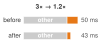
Component speedup rarely survives as end-to-end benchmark speedup.

Knowing what to measure, however, is only half the problem. Measuring incorrectly (with the wrong workloads, biased baselines, or uncontrolled variables) produces numbers that feel precise but mislead decisions. The history of computing benchmarking is littered with examples of technically sound metrics applied with flawed methodology, from compiler-gamed Whetstone scores to cherry-picked GPU benchmarks that predict nothing about sustained workloads. Understanding how measurement methodology evolved, and where it failed, is essential for designing benchmarks that distinguish genuine improvements from measurement artifacts.

The historical foundations of benchmarking² matter because they expose the validation failures that still recur in ML: optimized metrics that stop predicting real workloads, hardware numbers that ignore sustained operating state, and model scores that miss deployment cost. The same validation sequence governs modern practice: first verify that hardware delivers promised performance, then verify that the model and data optimizations built atop that hardware deliver their promised gains.

² Benchmark: From surveying, where a “bench mark” was a horizontal cut in stone serving as a fixed elevation reference. The term entered computing in the 1970s to describe standardized comparison points, but the surveying metaphor carries a systems lesson: just as an elevation measurement is meaningless without a calibrated reference, an ML throughput number is meaningless without controlled workloads, thermal state, and precision settings.

Self-Check: Question

1. In the three-dimensional ML benchmarking framework, what distinct failure mode does system benchmarking isolate compared to model and data benchmarking?

   1. Whether hardware accelerators, memory subsystems, and software runtimes deliver expected computational throughput and latency under workload execution patterns
   2. Whether model compression techniques preserve confidence calibration and accuracy on rare edge cases
   3. Whether the training dataset contains sufficient coverage, demographic balance, and resistance to covariate drift
   4. Whether human labeling errors and noisy annotations degrade model convergence rates

2. An ML serving pipeline has a baseline end-to-end request latency of \(50\text{ ms}\), of which the neural network inference model stage takes \(10\text{ ms}\) (the remaining \(40\text{ ms}\) is spent in request parsing, database feature fetching, image decoding, and response formatting). If the engineering team applies hardware acceleration to achieve a \(3\times\) speedup on the model inference stage alone, what is the resulting end-to-end pipeline speedup?

   1. Exactly \(3.0\times\) speedup
   2. Approximately \(1.2\times\) speedup (latency drops from \(50\text{ ms}\) to roughly \(43.3\text{ ms}\))
   3. Approximately \(2.1\times\) speedup (latency drops from \(50\text{ ms}\) to roughly \(23.8\text{ ms}\))
   4. No speedup (\(1.0\times\)) because non-model stages cancel out accelerator gains

3. True or False: Because ML benchmarks provide standardized datasets and metric formulas, a top-ranking benchmark score represents a permanent, universal verification of a model’s operational capability in production.

4. The ratio of sustained floating-point throughput achieved by an ML workload to the theoretical peak floating-point capability of the underlying hardware accelerator is known as Model FLOPs Utilization, abbreviated as ____.

5. Explain how Goodhart’s Law applies to ML systems benchmarking, and describe a concrete scenario where optimizing exclusively for a benchmark metric degrades real-world deployment quality.

See Answers →

Historical Foundations

In 1976, when Whetstone became one of the first standardized computing benchmarks, vendors began optimizing their compilers specifically for its floating-point tests, producing impressive numbers that did not reliably predict real application performance. Similar gaming has affected later benchmark generations. Understanding why ML benchmarking requires a three-dimensional approach demands tracing how measurement methodologies evolved, and often failed, over decades of computing history. Each generation of benchmarks emerged from the limitations of its predecessors, teaching lessons that directly inform modern ML evaluation.

Before that history begins, one boundary condition matters: a benchmark is useful only when it names the layer whose claim it validates.

Systems Perspective 1.2: Benchmarking as cross-layer evidence

An ML benchmark is meaningful only when it identifies which layer of the system is being validated. Data selection metrics such as PPD, area under the learning curve (AULC), and data compression ratio (DCR), all developed in Data Selection, measure whether fewer examples can preserve learning signal. Compression metrics (Model Compression) measure whether fewer parameters or lower precision preserve quality. Hardware metrics such as roofline position and TOPS/W (Hardware Acceleration) measure whether the machine executes the workload efficiently. The system benchmarks in section 1.3.2 through section 1.9.4 connect these layers by testing whether local improvements survive in an end-to-end workload.

That cross-layer role explains why benchmark history matters: each generation of performance measurement advanced when practitioners discovered that the previous method failed to predict real-world behavior. The evolution from simple performance metrics to ML benchmarking reveals three methodological shifts.

Performance benchmarks

The earliest computing benchmarks revealed a problem that plagues evaluation to this day: benchmark gaming. Whetstone (Curnow and Wichmann 1976) used a synthetic mix of scientific-program operations, while LINPACK³ (Dongarra et al. 1979) measured dense linear-system solving. Vendors could optimize specifically for such fixed tests rather than for broader workloads. SPEC CPU (1989) broadened evaluation through a suite of portable, application-oriented programs (Dixit 1993). This lesson directly shapes ML benchmarking: optimization claims from Model Compression require validation on representative tasks, and MLPerf’s inclusion of models such as ResNet-50 and BERT captures more of the deployment stack than an isolated kernel.

³ Whetstone and LINPACK: Whetstone (Curnow and Wichmann 1976) was named after the English Electric facility in Whetstone, Leicestershire, where the original ALGOL compiler was built; LINPACK (Dongarra et al. 1979) was a package and benchmark for dense linear systems, later used by the Top500 list. Whetstone’s fixed synthetic program mix and LINPACK’s dense linear-algebra focus made each useful but narrower than a diverse application suite. ML benchmarking inherited the same vulnerability: model-specific kernel tuning can overfit a single workload, which is why MLPerf uses multiple workloads spanning vision, language, and recommendation (Mattson et al. 2020; Reddi et al. 2019).

Curnow, H. J., and B. A. Wichmann. 1976. “A Synthetic Benchmark.” The Computer Journal 19 (1): 43–49. https://doi.org/10.1093/comjnl/19.1.43.

Dongarra, J. J., J. R. Bunch, C. B. Moler, and G. W. Stewart. 1979. LINPACK Users’ Guide. SIAM. https://doi.org/10.1137/1.9781611971811.

Dixit, Kaivalya M. 1993. “Overview of the SPEC Benchmarks.” In The Benchmark Handbook for Database and Transaction Systems, 2nd ed., edited by Jim Gray. Morgan Kaufmann.

As deployment contexts diversified, a second limitation emerged: single-metric evaluation proved inadequate. Graphics benchmarks began measuring rendering quality alongside frame rate; mobile benchmarks added battery life as a co-equal concern with performance. The multi-objective challenges from Introduction (balancing accuracy, latency, and energy) manifest directly in ML evaluation, where no single metric captures deployment viability.

A third shift occurred when distributed computing revealed that component-level optimization fails to predict system-level performance. A CPU benchmark cannot predict cluster throughput when network communication dominates. ML training similarly depends on the interplay of accelerator compute (Hardware Acceleration), data pipelines, gradient synchronization, and storage throughput. MLPerf evaluates complete workflows, recognizing that performance emerges from component interactions, not from components in isolation.

DAWNBench (Coleman et al. 2019) emerged as an early ML benchmark that pioneered time-to-accuracy evaluation, directly influencing MLPerf’s methodology for measuring training efficiency. These lessons culminate in MLPerf⁴ (2018), which synthesizes representative workloads, multi-objective evaluation, and integrated measurement while addressing ML-specific challenges (Mattson et al. 2020; Reddi et al. 2019).

Coleman, Cody, Deepak Narayanan, Daniel Kang, Tian Zhao, Jian Zhang, Luigi Nardi, Peter Bailis, Kunle Olukotun, Christopher Ré, and Matei Zaharia. 2019. “Analysis of DAWNBench, a Time-to-Accuracy Machine Learning Performance Benchmark.” ACM SIGOPS Operating Systems Review 53 (1): 14–25. https://doi.org/10.1145/3352020.3352024.

⁴ MLPerf: Launched in 2018 by a consortium of industry and academic institutions, MLPerf takes its name from “ML” combined with “Perf” (performance), echoing SPEC’s benchmarking tradition. MLPerf’s design principles—representative workloads, full-system measurement, and open submission—directly address the gaming that plagued Whetstone and LINPACK: vendors who could previously report peak kernel throughput on cherry-picked problem sizes must now report end-to-end system performance on standardized tasks (Mattson et al. 2020; Reddi et al. 2019).

Energy benchmarks

The multi-objective evaluation paradigm naturally extended to energy efficiency as computing diversified beyond mainframes with less constrained power budgets. Mobile devices demanded battery life optimization, while warehouse-scale systems faced energy costs rivaling hardware expenses. This shift established energy as a first-class metric alongside performance, spawning benchmarks like SPEC Power⁵ for servers and Green500⁶ for supercomputers.

⁵ SPEC Power: Introduced in 2007, SPEC Power measures performance per watt across 11 load levels from idle (0 percent) through 100 percent in 10 percent increments (Lange 2009). This granularity matters for ML serving: inference workloads rarely sustain 100 percent load, and servers that are efficient at peak but wasteful at partial load inflate the energy cost of real-world deployment.

Lange, Klaus-Dieter. 2009. “Identifying Shades of Green: The SPECpower Benchmarks.” IEEE Computer 42 (3): 95–97. https://doi.org/10.1109/mc.2009.84.

⁶ Green500: Started in 2007 as a counterpart to the Top500, Green500 ranks systems by FLOP/s per watt rather than raw performance (Feng and Cameron 2007). Its lesson for ML systems is methodological: the most cost-effective training cluster is not necessarily the fastest one, but the system that delivers useful work per watt under the workload and measurement boundary that matter.

Feng, Wu-chun, and Kirk W. Cameron. 2007. “The Green500 List: Encouraging Sustainable Supercomputing.” Computer 40 (12): 50–55. https://doi.org/10.1109/MC.2007.445.

MLCommons. 2024b. MLPerf Power Measurement.

Diverse workload patterns and system configurations continue to challenge power benchmarking across computing environments. MLPerf Power (MLCommons 2024b) addresses this with specialized methodologies for measuring the energy impact of machine learning workloads, reflecting energy efficiency’s central role in AI system design.

Energy benchmarking extends beyond hardware power measurement to include algorithmic efficiency. Model compression techniques (pruning, quantization, knowledge distillation) can reduce energy by changing the work a system performs, not only by changing the hardware that performs it. MobileNet-family architectures use depthwise separable convolutions to cut computation relative to heavier convolutional neural network (CNN) baselines such as ResNet (Howard et al. 2017; Sandler et al. 2018; He et al. 2016). These techniques, detailed in Model Compression, establish that energy-aware benchmarking must evaluate algorithmic efficiency alongside hardware power consumption; Energy costs quantifies the specific energy breakdown of INT8 vs. FP32. As AI systems scale, this lesson becomes central to sustainable computing practices.

Howard, A. G., M. Zhu, B. Chen, D. Kalenichenko, W. Wang, T. Weyand, M. Andreetto, and H. Adam. 2017. “MobileNets: Efficient Convolutional Neural Networks for Mobile Vision Applications.” CoRR abs/1704.04861.

Domain-specific benchmarks

As computing diversified beyond general-purpose servers, generic benchmarks proved inadequate for specialized domains. Three categories of specialization drove this evolution, each exposing measurement dimensions that general-purpose benchmarks could not address.

Deployment constraints shape core metric priorities. Data center workloads optimize for throughput with rack- and cluster-scale power budgets, while mobile AI operates within tight device thermal envelopes, and IoT devices require milliwatt-scale operation. These constraints, rooted in efficiency principles from Introduction, determine whether benchmarks prioritize total throughput or energy per operation.

Application requirements then impose functional and regulatory constraints beyond raw performance. Healthcare AI demands interpretability metrics alongside accuracy; financial systems may require very low latency with audit compliance; autonomous vehicles need safety-critical reliability and formal functional-safety validation. These requirements extend evaluation beyond traditional performance metrics; Responsible Engineering later systematizes the responsible-engineering principles behind fairness, interpretability, and compliance.

Operational conditions determine real-world viability. Autonomous vehicles face wide temperature ranges and degraded sensor inputs; data centers handle large concurrent request volumes with network faults; industrial IoT endures long deployments without maintenance. The hardware capabilities from Hardware Acceleration only deliver value when validated under these conditions.

Machine learning exemplifies this transition to domain-specific evaluation. Traditional CPU and GPU benchmarks prove insufficient for assessing ML workloads, which involve complex interactions between computation, memory bandwidth, and data movement patterns. MLPerf provides standardized performance measurement for machine learning models across these categories: MLPerf Training addresses data center deployment constraints with multi-node scaling benchmarks (Mattson et al. 2020), MLPerf Inference evaluates latency-critical application requirements across server to edge deployments (Reddi et al. 2019), MLPerf Tiny assesses ultra-constrained operational conditions for microcontroller deployments (Banbury et al. 2021), and a cross-cutting MLPerf Power track measures energy efficiency under each of these regimes. Reading table 1 down its constraint column shows tighter limits as deployment scale shrinks: data-center interconnect bandwidth gives way to latency service level agreements (SLAs) at server and edge, then to ultra-low-power operation with kilobytes of memory on microcontrollers. The same three-category framework, applied to each scale, produces a suite whose metrics track what actually limits the system at that scale rather than a single universal score.

Table 1: MLPerf Benchmark Suite Variants: Each variant addresses a different deployment context, from data-center-scale training to ultra-constrained microcontroller inference, targeting specific operational constraints and measuring metrics relevant to its deployment scenario.

MLPerf Variant	Target Domain	Key Constraints	Primary Metrics
MLPerf Training	Data center	Multi-node scaling, high bandwidth interconnects	Time-to-quality, throughput (samples/sec)
MLPerf Inference	Server/Edge	Latency SLAs, throughput requirements	QPS, latency percentiles, accuracy preservation
MLPerf Tiny	MCU/IoT	Ultra-low-power inference, limited memory	Latency, accuracy, energy per inference
MLPerf Power	Cross-cutting	Energy budgets, thermal constraints	Performance/W, energy per query

MLPerf Power extends the same discipline to energy efficiency, where the benchmarked quantity is useful work per watt rather than raw throughput alone. Domain-specific benchmarks drive targeted hardware and software optimizations while ensuring that improvements translate to deployment success rather than narrow laboratory conditions.

This historical progression, from general computing benchmarks through energy-aware measurement to domain-specific evaluation frameworks, provides the foundation for understanding ML benchmarking challenges. The lessons learned (representative workloads over synthetic tests, multi-objective over single metrics, integrated systems over isolated components) directly shape AI system evaluation. Table 2 summarizes this progression and the key lessons each generation contributed.

These lessons culminate in ML benchmarking suites, yet ML systems add statistical and data-dependent variability to the sources of system noise found in other workloads. They must satisfy all three historical lessons (representative workloads, multi-objective evaluation, integrated measurement) while also accounting for outcomes that vary with training data, weight initialization, and operation ordering. This additional variability requires corresponding statistical controls.

Individual organizations learned these lessons independently, often painfully, but isolated measurements cannot drive an industry. When one team measures inference latency including preprocessing and another excludes it, when accuracy benchmarks use different data splits, or when power measurements draw different system boundaries, the resulting numbers are incommensurable. The transition from ad-hoc measurement to standardized benchmarking suites transforms benchmarking from an internal validation exercise into a shared language that enables hardware procurement, architecture comparison, and deployment decisions across organizations.

Table 2: Benchmark Evolution: Evolution of computing benchmarks from synthetic operations to ML-specific evaluation. Each generation addressed limitations of its predecessors, culminating in MLPerf’s synthesis of representative workloads, multi-objective metrics, and integrated system measurement.

Benchmark	Year	Primary Focus	Key Metric(s)	Lesson for ML Benchmarking
Whetstone	1976	Synthetic floating-point operations	MWIPS	Gaming synthetic tests undermines evaluation validity
LINPACK	1979	Linear algebra (matrix operations)	FLOP/s	Isolated operations miss system-level complexity and bottlenecks
SPEC CPU	1989	Real application workloads	SPECrate, SPECspeed	Representative workloads reveal true deployment performance
SPEC Power	2007	Server energy efficiency	ssj_ops/W across load levels	Energy efficiency requires multi-load evaluation, not just peak performance
Green500	2007	HPC energy efficiency	GFLOP/s per watt	Efficiency rankings complement raw performance rankings
MLPerf	2018	ML systems (training + inference)	Time-to-quality, QPS, latency, accuracy	Synthesizes all lessons: representative workloads + multi-objective + system

Self-Check: Question

1. Why did computing benchmark methodology historically transition away from synthetic instruction-mix microbenchmarks (such as Whetstone and Dhrystone) to representative application suites (such as SPEC CPU)?

   1. Synthetic microbenchmarks required too much memory bandwidth to execute on modern microprocessors
   2. Representative application suites were easier to implement and did not require source code compilation
   3. Synthetic benchmarks lacked realistic memory access patterns and branch behavior, allowing optimizing compilers to artificially game scores via dead-code elimination and loop unrolling
   4. Hardware vendors refused to publish floating-point operations per second for synthetic loops

2. How do the constraints and primary evaluation metrics differ across the domain-specific variants of the MLPerf benchmark suite?

   1. All MLPerf variants evaluate identical metrics (pure TFLOPS) across different hardware form factors
   2. MLPerf Training focuses on latency SLAs, while MLPerf Inference evaluates multi-node interconnect bandwidth
   3. MLPerf Tiny measures data center power consumption, while MLPerf Power evaluates floating-point peak throughput
   4. MLPerf Training targets multi-node cluster scaling and time-to-quality, MLPerf Inference evaluates latency SLAs and QPS across server and edge, MLPerf Tiny targets microwatt-scale energy and memory constraints on microcontrollers, and MLPerf Power measures performance-per-watt

3. True or False: The introduction of energy-efficiency benchmarks like SPECpower and Green500 replaced raw throughput benchmarks, because computing systems are now evaluated solely on Joules per operation.

4. Explain how the historical evolution of computer benchmarking—from synthetic instruction loops to SPEC suites and Green500—directly informed the core design principles of MLPerf.

5. Order the following historical computing benchmark paradigms chronologically from earliest to most modern:

1. Standardized domain-specific ML consortium suites (e.g., MLPerf) with multi-scenario serving and strict convergence run rules
2. Synthetic instruction-mix microbenchmarks (e.g., Whetstone, Dhrystone) measuring isolated arithmetic throughput
3. Multi-organization application suites (e.g., SPEC CPU) evaluating real-world compiler and scientific workloads
4. High-Performance Computing dense linear algebra factorization benchmarks (e.g., LINPACK / TOP500)
5. Multi-load energy efficiency and server power benchmarks (e.g., SPECpower_ssj2008, Green500)

See Answers →

System Benchmarking Suites

A team evaluating edge deployment hardware needs to compare five different system on chip (SoC) designs for a smart camera product. Vendor A reports 8 TOPS at INT8; Vendor B reports 15 TOPS at INT4; Vendor C reports inference latency on a proprietary model; Vendor D cites MLPerf scores from two generations ago; Vendor E provides only peak throughput at maximum batch size. None of these numbers are comparable. The team cannot make a procurement decision because every vendor measured a different thing, under different conditions, using different definitions of “performance.” The problem is not a lack of data but a lack of commensurable data, and benchmarking suites exist to solve exactly this fragmentation.

Three lessons from benchmark history (representative workloads, multi-objective evaluation, and integrated measurement) converge with the challenge unique to ML: inherent probabilistic variability. Modern benchmarking suites encode these lessons into standardized frameworks that make the kind of cross-organization comparison the hardware procurement team needs possible.

ML benchmarks must evaluate the interplay between algorithms, hardware, and data, not merely computational efficiency alone. Early benchmarks focused on algorithmic performance (LeCun et al. 1998), but scaling demands expanded the focus to hardware efficiency (Jouppi et al. 2017), and high-profile deployment failures elevated data quality as a third evaluation dimension (Gebru et al. 2021). This probabilistic nature elevates accuracy to a first-class evaluation dimension alongside speed and energy consumption: the same ML system can produce different results depending on the data it encounters. Energy efficiency cuts across all three framework dimensions, since algorithmic choices affect computational complexity (Hernandez and Brown 2020), hardware capabilities determine energy-performance trade-offs, and dataset characteristics influence training energy costs.

Jouppi, Norman P., Cliff Young, Nishant Patil, David Patterson, Gaurav Agrawal, Raminder Bajwa, Sarah Bates, et al. 2017. “In-Datacenter Performance Analysis of a Tensor Processing Unit.” Proceedings of the 44th Annual International Symposium on Computer Architecture, ISCA ’17, 1–12. https://doi.org/10.1145/3079856.3080246.

Gebru, Timnit, Jamie Morgenstern, Briana Vecchione, Jennifer Wortman Vaughan, Hanna Wallach, Hal Daumé III, and Kate Crawford. 2021. “Datasheets for Datasets.” Communications of the ACM 64 (12): 86–92. https://doi.org/10.1145/3458723.

Hernandez, Danny, and Tom B. Brown. 2020. “Measuring the Algorithmic Efficiency of Neural Networks.” arXiv Preprint arXiv:2005.04305, ahead of print. https://doi.org/10.48550/arxiv.2005.04305.

ML measurement challenges

ML systems combine several sources of measurement variability that many traditional benchmarks were not designed to evaluate together. These include algorithmic randomness from weight initialization and data shuffling, hardware thermal states that affect clock speeds, system load variation from concurrent processes, and environmental factors such as network conditions and power management. Rigorous statistical methods are needed to distinguish genuine performance improvements from this measurement noise.

To address this variability, effective benchmark protocols require repeated experimental runs with random seeds chosen for the study design. The number of runs should follow the required uncertainty or statistical-power target, with measures beyond simple means (including standard deviations or confidence intervals) reported to quantify stability and distinguish genuine improvements from measurement noise.

Empirical studies have shown how inadequate statistical rigor can lead to misleading conclusions. Reinforcement-learning gains often fall within statistical noise (Henderson et al. 2018), while generative adversarial network comparisons often lack controlled experimental protocols, producing inconsistent rankings across seeds (Lucic et al. 2018). These findings underscore the importance of establishing measurement protocols that account for ML’s probabilistic nature.

Lucic, Mario, Karol Kurach, Marcin Michalski, Sylvain Gelly, and Olivier Bousquet. 2018. “Are GANs Created Equal? A Large-Scale Study.” Advances in Neural Information Processing Systems (NeurIPS) 31.

A 1K test set cannot reliably see a one-point regression.

Napkin Math 1.1: The statistical confidence trap

Problem: A baseline classifier scores 95 percent, while a compressed version scores 94 percent on 1,000 images. Does this one-point drop establish a regression?

Math:

1. Expected errors: The scores correspond to 50 errors and 60 errors. Under the baseline binomial model, the error count has a standard deviation of about 7 errors.

2. Difference interval (95 percent): Let \(\hat p_1\) and \(\hat p_2\) denote the baseline and compressed accuracy estimates, respectively, and let \(N\) be the number of images evaluated for each model. Treating the two estimates as independent, the standard error of their difference is

   \[ \operatorname{SE}(\hat p_1-\hat p_2) = \sqrt{\frac{\hat p_1(1-\hat p_1)}{N} + \frac{\hat p_2(1-\hat p_2)}{N}}. \]

   The observed 1 percentage point difference has an approximate interval from -1 percentage point to 3 percentage points, which includes zero.

   Implication: Because the interval includes zero, the result does not establish a one-point regression. If both models ran on the same images, retain their disagreement counts and use a paired test such as McNemar’s test; marginal accuracies are insufficient. The 1,825-sample estimate for a single rate with ±1 percentage point precision does not power this comparison.

Systems insight: Small benchmarks exhibit what amounts to a laboratory fallacy. The test set, viewed as a measurement instrument, must be sized to match the precision of the change it is meant to detect.

Representative workload selection determines benchmark validity. Synthetic microbenchmarks (which generate random uniform tensors in memory) often fail to capture the complexity of real ML workloads where data movement, memory allocation, and dynamic batching create performance patterns not visible in simplified tests. Conversely, trace-based benchmarking replays recorded production request traces—capturing realistic inter-arrival times, bursty arrival distributions, and variable sequence lengths—to stress-test serving infrastructure under true production conditions. Comprehensive benchmarking therefore requires workloads that reflect actual deployment patterns: variable sequence lengths in language models, mixed precision training regimes, and realistic data loading patterns that include preprocessing overhead.

Example 1.1: Goodhart's Law in action

Scenario: An engineering team optimizes an NMT translation model for offline BLEU score, increasing beam search size from 1 to 10.

Diagnosis: The larger beam search achieves a 0.5-point BLEU gain on paper but increases candidate evaluations by 10×, causing inference latency to explode from 50 ms to 200 ms (4× slowdown).

Systems lesson: Optimizing offline accuracy without latency constraints invites Goodhart’s Law failures. Production benchmarks must enforce strict service-level objectives (SLOs) for serving latency (e.g., latency < 100 ms).

Beyond workload representativeness, the distinction between statistical significance and practical significance requires careful interpretation. A small performance improvement might achieve statistical significance across hundreds of trials but prove operationally irrelevant if it falls within measurement noise or costs exceed benefits. This is the statistical confidence trap: seemingly rigorous evaluation still misleads.

Statistical confidence is a measurement-capacity problem: the benchmark may be pointed at the right quantity, but the test set is too small to resolve the change. A second failure mode is metric alignment. Here the measurement can be precise and reproducible, yet still reward behavior that violates the deployed system’s objective. The translation example makes that distinction concrete by showing how a BLEU improvement can come at the expense of latency.

These measurement failures share a deeper limitation: a benchmark on a static dataset measures recognition under a fixed distribution, not the robustness to a shifting one that production demands. The data dimension of the framework developed later in this chapter confronts exactly that gap.

These measurement challenges motivate evaluating each dimension of the three-dimensional framework (system, model, and data) with distinct methodologies. The bulk of this chapter focuses on system benchmarking (training benchmarks, inference benchmarks, and power measurement) because these form the foundation of standardized evaluation through MLPerf. Section 1.11 then develops the distinct methodologies required for model and data benchmarking.

System benchmarks

System benchmarks measure the computational foundation that enables model capabilities, examining how hardware architectures, memory systems, and interconnects affect overall performance. This validation is critical because hardware specifications often describe theoretical peaks that application workloads do not sustain. The discrepancy is common enough to make peak-performance claims incomplete. System benchmarks reveal these gaps by running standardized ML workloads rather than relying on peak arithmetic rates alone.

Systems Perspective 1.3: The fallacy of peak performance

Dave Patterson often refers to peak performance as “the performance the manufacturer guarantees you will not exceed.” For ML systems, the gap can be wide because of the memory wall: a memory-bound model leaves much of the advertised FLOP/s unreachable no matter how fast the arithmetic units run. Standardized benchmarks like MLPerf require systems to run specified models and data, revealing sustained performance at a documented operating point rather than a universal rate for every workload.

For memory-bound workloads, the peak-vs.-sustained gap follows from the memory wall; compute-bound workloads may approach peak. This distinction reframes vendor evaluation from guesswork into a checklist of concrete criteria.

Checkpoint 1.1: Decoding vendor benchmark claims

When evaluating hardware or software based on vendor-reported benchmarks, check whether the claim identifies the workload, measurement boundary, and operating conditions.

• Measured quantity: Does the latency number include preprocessing and postprocessing, not just model execution?
• Precision boundary: Can the precision behind a throughput claim, such as INT4 versus INT8 or FP16, be identified?
• Workload boundary: Are the model, batch size, and input distribution used to produce the comparison explicitly named?
• Excluded costs: Are memory transfers, model loading, initialization, sustained thermal behavior, and power accounted for at the claimed performance level?
• Claimed vs. achieved: Given a 1,000 TFLOP/s peak claim and a benchmark that sustains 350 TFLOP/s, estimate the MFU and state whether that utilization ratio alone identifies the bottleneck.

Engineers should reject any benchmark claim whose workload boundary, precision, and excluded costs cannot be reconstructed. A headline throughput or latency number becomes useful only after the engineer can map it to the actual model, batch shape, data movement, sustained operating point, and power envelope.

The underlying hardware—CPUs, GPUs, Tensor Processing Units (TPUs),⁷ and application-specific integrated circuits (ASICs)⁸—determines ML-system speed, efficiency, and scale. System benchmarks provide standardized methods for comparing hardware across AI workloads by computational throughput, memory bandwidth, power efficiency, operator coverage, and scaling (Reddi et al. 2019; Mattson et al. 2020).

⁷ TPU (tensor processing unit): Google’s custom ASIC for neural network workloads (architecture details in Hardware Acceleration). A TPU v4 pod (4,096 chips) delivers 1.1 exaFLOP/s peak BF16 (Jouppi et al. 2023), but benchmarking TPUs requires caution: their systolic-array architecture favors regular tensor operations, so peak FLOP/s overstate performance on irregular workloads like sparse attention or dynamic control flow.

Jouppi, Norm, George Kurian, Sheng Li, Peter Ma, Rahul Nagarajan, Lifeng Nai, Nishant Patil, et al. 2023. “TPU v4: An Optically Reconfigurable Supercomputer for Machine Learning with Hardware Support for Embeddings.” Proceedings of the 50th Annual International Symposium on Computer Architecture, 1–14. https://doi.org/10.1145/3579371.3589350.

⁸ ASIC (application-specific integrated circuit): An ASIC’s peak TOPS number applies only to the specific operators it was designed for. A single unsupported layer forces fallback to a general-purpose processor, potentially negating the entire efficiency advantage. This makes operator coverage the first question in any ASIC benchmark: the gap between peak and achieved throughput is not a hardware limitation but a workload-compatibility limitation.

Table 3 translates common marketing phrases into the technical caveats behind each.

Table 3: Decoding Vendor Benchmark Claims: Four common marketing phrases and the technical caveats that determine whether a claim describes end-to-end performance, a narrow accelerator measurement, or an unsupported efficiency comparison.

Vendor Claim	What It Often Means
“Up to 10,000 images/sec”	Peak throughput at maximum batch size, INT8, without preprocessing
“Sub-millisecond latency”	Accelerator compute only, excluding data transfer
“5\(\times\) more efficient”	Per-operation efficiency, not total system efficiency
“Optimized for AI”	May only accelerate specific operations or precisions

System benchmarks serve two functions. For practitioners, they enable informed hardware selection by providing comparative data across configurations. For manufacturers, they quantify generational improvements and guide accelerator development. As GPU adoption grew, accuracy also improved rapidly, illustrating how hardware and algorithmic advances can drive progress together.

Definition 1.2: Machine learning system benchmarks

Machine learning system benchmarks are standardized evaluation protocols that hold the workload and quality target constant while varying the hardware-software stack, measuring \(\eta_{\text{hw}} = R_{\text{sustained}} / R_{\text{peak}}\) and \(L_{\text{lat}}\) to isolate infrastructure efficiency from algorithmic improvements.

1. Significance: The same ResNet-50 model can deliver very different throughput across hardware stacks, precision formats, batch sizes, and compiler configurations, yet still report the same ImageNet Top-1 accuracy. System benchmarks capture this implementation gap, which is invisible to algorithmic benchmarks that only report accuracy.
2. Distinction: Unlike algorithmic benchmarks (which vary model architectures and training procedures to improve convergence accuracy), system benchmarks hold the algorithm fixed and vary the implementation (kernel libraries, quantization formats, batch sizes, and hardware generations) to measure how efficiently the hardware-software stack executes the iron law’s \(O/(R_{\text{peak}} \cdot \eta_{\text{hw}})\) term.
3. Common pitfall: A frequent misconception is that a system benchmark result generalizes across workloads. An accelerator that achieves high utilization on ResNet-50 (a compute-friendly vision workload) may achieve much lower utilization on a recommendation system (a memory-bandwidth-bound workload). System benchmarks are workload-specific; no single metric characterizes a hardware platform.

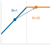
Larger batches push transformer inference from memory-bound to compute-bound.

⁹ FLOP/s (floating-point operations per second): The gap between advertised peak FLOP/s and achieved FLOP/s is the central tension in hardware benchmarking. The A100 advertises 312 TFLOP/s FP16 Tensor Core, but real workloads achieve different fractions of peak depending on arithmetic intensity, memory access patterns, precision, and runtime overhead. Reporting peak FLOP/s without utilization context is the most common benchmarking distortion.

Effective benchmark interpretation requires knowing the performance characteristics of target hardware. Whether a specific AI workload is compute bound or memory-bound provides essential insight for optimization decisions. Computational intensity, measured as FLOP/byte,⁹ determines performance limits. Consider an NVIDIA A100 GPU with 312 TFLOP/s of FP16 Tensor Core performance (FP32 is 19.5 TFLOP/s) and 2.04 TB/s memory bandwidth (SXM variant). Dividing peak compute by peak bandwidth yields an arithmetic intensity threshold of 153 FLOP/byte. Workloads below this threshold are bottlenecked by memory bandwidth, while those above are bottlenecked by compute capacity. The Roofline Model in Roofline Model provides the architectural foundation for interpreting these benchmark results. The Roofline model derives the roofline equation and the ridge-point threshold from first principles, so the arithmetic intensity bound used here can be reconstructed for any accelerator.

Roofline position¹⁰ depends on the workload. In this worked A100 example, an illustrative high-intensity ResNet-50 forward-pass workload at large batch size uses an arithmetic intensity of ~300 FLOP/byte, above the A100 ridge, and therefore represents compute-bound kernels (He et al. 2016; Choquette et al. 2021). Lower-intensity operations fall below the ridge into the memory-bound regime: a BERT inference at batch size one, counting only weight-loading traffic, reaches ~100 FLOP/byte arithmetic intensity and a lower performance ceiling than peak. Increasing the batch size moves that same workload across the ridge from memory-bound to compute-bound (Pope et al. 2023). A concrete example: The A100 analysis works the intensity-to-utilization calculation end to end on the A100, contrasting a compute-bound matrix multiplication kernel against a memory-bound element-wise kernel, so the steps generalize to any model-hardware pair.

¹⁰ Roofline model: Williams et al. (2009) introduced the Berkeley model, named for the visual shape of its performance ceiling. Its ridge point (peak FLOP/s divided by peak bandwidth) separates memory-bound from compute-bound workloads, showing whether optimization should target data movement or arithmetic.

Williams, Samuel, Andrew Waterman, and David Patterson. 2009. “Roofline: An Insightful Visual Performance Model for Multicore Architectures.” Communications of the ACM 52 (4): 65–76. https://doi.org/10.1145/1498765.1498785.

Choquette, Jack, Wishwesh Gandhi, Olivier Giroux, Nick Stam, and Ronny Krashinsky. 2021. “NVIDIA A100 Tensor Core GPU: Performance and Innovation.” IEEE Micro 41 (2): 29–35. https://doi.org/10.1109/mm.2021.3061394.

Pope, Reiner, Sholto Douglas, Aakanksha Chowdhery, Jacob Devlin, James Bradbury, Jonathan Heek, Kefan Xiao, Shivani Agrawal, and Jeff Dean. 2023. “Efficiently Scaling Transformer Inference.” Proceedings of Machine Learning and Systems (MLSys) 5: 606–24.

A worked BERT inference estimate shows how these roofline principles translate into concrete deployment predictions.

Napkin Math 1.2: Roofline analysis for BERT inference

Problem: BERT-Base must be deployed for inference on an A100 GPU. Management expects high GPU utilization. What performance should be predicted, and how can it be improved?

Step 1: Hardware limits.

• Peak compute: 312 TFLOP/s (FP16 Tensor Core)
• Memory bandwidth: 2.04 TB/s
• Ridge point: 312 TFLOP/s ÷ 2.04 TB/s = 153 FLOP/byte

Any workload with arithmetic intensity below 153 FLOP/byte is memory bound; above is compute bound.

Step 2: BERT-base characteristics.

• Parameters: 110M = 220 MB (FP16)
• FLOPs per inference: ~22 GFLOP (forward pass with sequence length \(S=128\))
• Data movement: ~220 MB (must load all weights from memory)
• Arithmetic intensity: \((22 \times 10^{9}) \div (220 \times 10^{6})\) = 100 FLOP/byte (weights-only model; see note in main text)

Step 3: Performance prediction. Since 100 FLOP/byte < 153 FLOP/byte, BERT at batch = 1 is memory bound: \[\begin{gather*} \text{Achievable perf} = \text{100 FLOP/byte} \times \text{2.04 TB/s} = \text{203.9 TFLOP/s} \\ \text{GPU utilization} = \text{203.9 TFLOP/s} / \text{312 TFLOP/s} = \text{$65.4\%$} \end{gather*}\]

Step 4: Optimization via batching. Increase batch size to 32:

• Same 220 MB of weights, but 32× more compute
• New FLOPs: \(22 \times 10^{9} \times 32\) = 704 GFLOP
• New intensity: \((704 \times 10^{9}) \div (220 \times 10^{6})\) = 3200 FLOP/byte

Since 3200 FLOP/byte > 153 FLOP/byte, batch = 32 is compute bound. Assuming the implementation then sustains 85 percent of peak: \[\begin{gather*} \text{Achievable perf} \approx \text{$85\%$} \times \text{312 TFLOP/s} = \text{265.2 TFLOP/s} \\ \text{GPU utilization} \approx 85\% \end{gather*}\] Systems insight: Batch size can transform memory-bound inference into compute-bound inference by raising arithmetic intensity. The displayed 85 percent is an implementation-efficiency assumption, not a roofline prediction. Batching also increases latency because the system must wait to accumulate requests. This is the fundamental throughput-latency trade-off that MLPerf scenarios capture: SingleStream (batch = 1, latency-optimized) vs. Offline (maximum batch, throughput-optimized).

System benchmarks evaluate performance across scales, ranging from single-chip configurations to large distributed systems and covering both training and inference. Figure 1 juxtaposes sourced ImageNet top-5 error rates (Russakovsky et al. 2015; Krizhevsky et al. 2012) with a reconstruction of the growing use of GPUs in challenge entries, read from the entry counts NVIDIA charted for the challenge (Gray 2015). The two series show contemporaneous trends, not a causal estimate of how much of the accuracy improvement came from hardware rather than algorithms, data, or training practice.

\begin{tikzpicture}[font=\small\sffamily]

\pgfplotsset{myaxis/.style={
  axis line style={draw=none},
  /pgf/number format/.cd,
  1000 sep={},
   width=105mm,
   height=60mm,
   axis lines=left,
   axis line style={thick,-latex},
    tick label style={/pgf/number format/assume math mode=true},
    yticklabel style={font=\fontsize{7pt}{7}\selectfont\sffamily,
    /pgf/number format/.cd, fixed, fixed zerofill, precision=1},
    xticklabel style={font=\fontsize{7pt}{7}\selectfont\sffamily},
    ylabel style={font=\footnotesize\sffamily},
    xlabel style={font=\footnotesize\sffamily},
    y tick style={draw=none},
    x tick style={draw=none,thin},
    tick align=outside,
    major tick length=1mm,
    title style={yshift=-4pt,font=\footnotesize\sffamily},
    xmin=2009.5,xmax=2014.5,
    xtick={2010,2011,2012,2013,2014},
    }}
  %grid
\begin{axis}[myaxis,
    grid=both,
    major grid style={thin,black!60},
    minor tick num=1,
    ymin=0,    ymax=33,
    ytick={0,10,...,30},
    xticklabels={,,,,},
]
\end{axis}
%bar
\begin{axis}[myaxis,
    axis y line*=right,
    axis x line=none,
    ylabel={\color{green!60!black}\# of Entries Using GPUs},
    xlabel={Year},
    ymin=0,    ymax=133,
    ytick={0,25,...,125},
    every axis plot/.append style={
          ybar,
          bar width=0.55,
          bar shift=0pt,
          fill
        }]
      \addplot[draw=none]coordinates {(2010,0)};
      \addplot[draw=none]coordinates {(2011,0)};
      \addplot[green!60!black]coordinates {(2012,4)};
      \addplot[green!60!black]coordinates{(2013,60)};
      \addplot[green!60!black]coordinates{(2014,110)};
      %
\end{axis}
  %line
\begin{axis}[myaxis,
    ylabel={\color{blue!50!black}Top-5 Error Rate (\%)},
    xlabel={Year},
    ymin=0,    ymax=33,
    ytick={0,10,...,30},
    xticklabels={2010,2011,2012,2013,2014},
]
\addplot[
  mark=*,
  mark size=2pt,
  line width=1.5pt,
  draw=blue!50!black, %
  mark options={fill=red, draw=red} %
]
table[x=Year,y=Y, col sep=comma] {
Year,Y
  2010,28.2
  2011,25.8
  2012,16.4
  2013,11.7
  2014,7.3
};
\end{axis}
\end{tikzpicture}

Figure 1: ImageNet Error and GPU Adoption: Sourced top-5 error rates are shown beside GPU use among challenge entries. The temporal association does not isolate hardware’s causal contribution. Error-rate sources: (Russakovsky et al. 2015; Krizhevsky et al. 2012). Gray (2015) charts the per-year GPU entry counts.

Gray, Allison. 2015. NVIDIA and IBM Cloud Support ImageNet Large Scale Visual Recognition Challenge. NVIDIA Technical Blog.

The ImageNet example places GPU adoption alongside falling error rates without isolating either contribution; section 1.11.1 revisits this progression through model-specific architectural milestones. Effective system benchmarking, however, requires understanding the relationship between workload characteristics and hardware utilization. Modern AI systems rarely achieve theoretical peak performance due to interactions between computational patterns, memory hierarchies, and system architectures. This gap between theoretical and achieved performance shapes the design of meaningful system benchmarks.

Realistic hardware utilization patterns are essential for actionable benchmark design. As the preceding roofline analysis illustrated, GPU utilization varies with batch size and model architecture; the compute-bound value of 85 percent is an assumption, while the memory-bound single-request value is 65.4 percent. These patterns extend to memory bandwidth: parameter-heavy transformer inference and activation-heavy convolutional workloads stress different parts of the memory hierarchy, directly impacting achievable performance across different precision levels.

Effective system benchmarks must measure realistic utilization rather than peak theoretical capability, and this requirement establishes several scope boundaries. Energy is one dimension: performance per watt varies widely across platforms, and an underutilized accelerator consumes disproportionate power for its output, penalizing both operational cost and environmental impact. Distribution is another: multi-node training adds communication bottlenecks, network-topology effects, and coordination overhead that single-node benchmarks cannot capture and that warrant dedicated treatment beyond this book. Within the single-machine scope here, multi-GPU benchmarking instead focuses on intra-node communication, memory-bandwidth utilization across accelerators, and gradient-synchronization efficiency across distinct accelerator memories connected by NVLink or PCIe. Across all of these, a benchmark earns its value only when its operating point matches the deployment’s, not the datasheet’s.

Community-driven standardization

The hardware utilization insights are only useful for comparison when measured consistently, which requires community-driven standardization. When one team measures inference latency with preprocessing included and another excludes it, when accuracy benchmarks use different data splits, or when power measurements employ different system boundaries, meaningful comparison becomes impossible. Individual organizations cannot establish measurement standards alone; the proliferation of benchmarks across the three dimensions creates fragmentation that only coordinated effort can resolve.

The most successful benchmarks emerge through broad collaboration among academic institutions, industry partners, and domain experts. ImageNet’s lasting impact demonstrates how sustained community engagement through workshops, challenges, and open datasets establishes authority that corporate-driven benchmarks rarely achieve. This collaborative development creates a foundation for formal standardization: IEEE working groups (IEEE Standards Association 2024) and ISO/IEC technical committees (ISO 2024) codify community-developed methodologies into official standards (for example, IEEE 2416 (IEEE Standards Association 2019) for system power modeling), providing precise measurement specifications that enable reliable cross-institutional comparison. Projects that provide open-source reference implementations, containerized evaluation environments, and comprehensive validation suites further reduce barriers and ensure consistent interpretation across research groups.

IEEE Standards Association. 2024. IEEE Standards Association: Working Groups for AI and ML.

ISO. 2024. ISO/IEC JTC 1/SC 42 Artificial Intelligence.

IEEE Standards Association. 2019. IEEE 2416-2019: Standard for Power Modeling to Enable System-Level Analysis.

ML benchmarks must balance academic rigor with industry practicality, since theoretical advances must translate to practical improvements in deployed systems (Mattson et al. 2020; Reddi et al. 2019). Benchmarks that emerge from this balance, with transparent governance and regular evolution, become durable reference points; those developed in isolation struggle to gain traction regardless of technical sophistication. These evaluation methodology principles guide both training and inference benchmark design throughout this chapter.

Community standards ensure reproducibility, but they do not prescribe the level of detail at which measurements should be taken. A benchmark could time a single matrix multiplication or an entire training run—and each choice reveals different kinds of information. The depth of measurement, from individual operations to complete systems, determines what insights benchmarks can provide and which problems they can diagnose.

Self-Check: Question

1. In roofline analysis, an accelerator has a peak compute performance of \(312\text{ TFLOPS}\) (BF16) and a memory bandwidth of \(2.0\text{ TB/s}\), yielding a machine ridge point of \(I_{\text{knee}} = 156\text{ FLOP/byte}\). When serving a Transformer model with batch size \(b=1\), the arithmetic intensity is only \(I = 4.8\text{ FLOP/byte}\). What is the maximum achievable compute utilization (MFU) on this workload?

   1. Approximately \(3.1\%\) of peak compute throughput (memory-bandwidth bound)
   2. Exactly \(100\%\) because modern tensor cores execute batch \(b=1\) at peak speed
   3. Approximately \(50\%\) due to pipeline bubbles and kernel launches
   4. Approximately \(85\%\) because matrix-vector multiplications are compute-bound

2. A vendor publishes a marketing claim stating their new AI accelerator achieves ‘\(120\text{ TFLOPS}\) on Transformer inference.’ Which combination of parameters is essential to make this throughput figure technically actionable and reproducible?

   1. Only the silicon process node (e.g., \(4\text{ nm}\)) and the data center room temperature
   2. Numerical precision (e.g., INT8 vs. FP16), batch size, sequence length, software/compiler stack version, and sustained thermal operating state
   3. The brand of server power supply and the serial number of the host CPU
   4. Only the parameter count of the model, without specifying batch size or precision

3. Explain why a single benchmark run is insufficient to characterize ML system performance, identifying at least two distinct hardware or runtime sources of execution variance.

4. Compare the primary objectives and constraints of the MLPerf Closed Division versus the Open Division.

5. Explain how community-driven benchmarking consortia prevent vendor gaming and establish commensurable evidence for hardware procurement.

6. Order the following steps in the MLPerf benchmark execution and verification lifecycle from first to last:

1. Submit execution logs, power traces, and configuration metadata to the MLCommons consortium
2. Execute unmeasured warm-up iterations to populate caches and stabilize operating temperatures
3. Lock down hardware frequencies, software environment, and driver configurations
4. Execute the standardized benchmark harness while logging timestamped execution and energy metrics
5. Undergo peer-review audit where competing organizations inspect logs for run-rule compliance
6. Run the compliance validation suite to verify prediction outputs meet the target accuracy threshold

See Answers →

Benchmarking Granularity

A GPU kernel that runs 3\(\times\) faster in isolation may deliver zero end-to-end speedup if the data pipeline cannot keep pace. This diagnostic failure makes evaluation granularity a fundamental design choice. Standardization specifies how measurement is consistent, while benchmarking granularity specifies what is measured. Each validation dimension can be assessed at different scales, from individual operations to complete workflows, with each granularity level revealing different kinds of problems:

• Micro benchmarks isolate individual components: kernel execution time, memory bandwidth utilization, single-layer accuracy. These diagnose where problems occur.
• Macro benchmarks evaluate subsystems: full model training convergence, inference pipeline throughput, dataset bias metrics. These reveal what problems exist.
• End-to-end benchmarks measure complete workflows: request-to-response latency including preprocessing, training time-to-accuracy including data loading, model performance on production data distributions. These show whether the system works.

The optimization techniques from Part III operate at different granularities (kernel fusion targets micro performance, pruning affects macro model behavior, data curation determines end-to-end generalization) and validation must match. A micro benchmark might show kernel speedup while a macro benchmark reveals memory bottlenecks that negate the gain; an end-to-end benchmark might expose data pipeline stalls invisible at any other level.

Figure 2 maps these granularity levels onto the ML stack by breaking the stack into four distinct evaluation scopes. Each scope progressively expands the measurement boundary. Micro-benchmarks isolate neural network layers, macro-benchmarks encompass complete models, application benchmarks add supporting compute, and end-to-end benchmarks capture the full deployment context including non-AI components.

\begin{tikzpicture}[font=\sffamily\small]
 \tikzset{%
 Box/.style={
 node distance=1.25,
    inner xsep=2pt,
    draw=RedLine,
    line width=0.75pt,
    fill=RedL!20,
    align=flush center,
    text width=30mm,
    minimum width=30mm, minimum height=10mm
  },
   Box2/.style={Box, draw=BlueLine,fill=BlueL!20},
   Box3/.style={Box, draw=GreenLine,fill=GreenL!40},
   Box4/.style={Box, draw=BrownLine,fill=BrownL!40,text width=24mm,},
 %
  Line/.style={line width=0.35pt,black!60,text=black},
  LineD/.style={line width=0.75pt,black!60,text=black,dashed,dash pattern=on 3pt off 2pt},
  Line2/.style={line width=0.85pt,black!60,text=black,-{Latex[length=6pt, width=4pt]}}
}

  \def\rows{3}
  \def\cols{4}
  \def\r{0.35}
  \def\xgap{0.15}
  \def\ygap{0.5}

\begin{scope}[local bounding box=CEN,shift={($(0,0)+(0,0)$)}]
  \foreach \i [count=\c] in {0,...,\numexpr\rows-1} {
    \foreach \j  in {0,...,\numexpr\cols-1} {
      \pgfmathtruncatemacro{\newX}{\j + 1} %
      % Circle position
      \pgfmathsetmacro\x{\j*(2*\r + \xgap)}
      \pgfmathsetmacro\y{-\i*(2*\r + \ygap)}
\definecolor{cellcol}{RGB}{253,226,240}
     \node[fill=VioletLine!60,circle,minimum size=\r](C\c\newX)at(\x,-\y){};
    }
  }
\foreach \a/\b in {C3/C2, C2/C1}{%
  \foreach \i in {1,2,3,4}{%
    \foreach \j in {1,2,3,4}{%
      \draw[Line] (\a\i) -- (\b\j);
    }%
  }%
}
\end{scope}
\scoped[on background layer]
\node[outer sep=0pt,draw=BackLine,inner xsep=3mm,inner ysep=2mm,yshift=0mm,
           fill=BackColor!20,fit=(C11)(C34),line width=0.75pt](BB1){};
\node[above=2pt of  BB1.north,anchor=south]{ML Layers};
%%%
\node[Box,below right =0.19 and 1.4 of BB1.north east](MA){Model A};
\node[Box,above right =0.19 and 1.4 of BB1.south east](MB){Model B};
\scoped[on background layer]
\node[outer sep=0pt,draw=BackLine,inner xsep=3mm,inner ysep=2mm,yshift=0mm,
           fill=BackColor!20,fit=(MA)(MB),line width=0.75pt](BB2){};
\node[above=2pt of  BB2.north,anchor=south]{ML Model};
%
\def\du{1.7}
\node[Box2,right =\du of MA](T1){AI Task 1};
\node[Box2, right =\du  of MB](T2){Supporting Compute};
\scoped[on background layer]
\node[outer sep=0pt,draw=BackLine,inner xsep=3mm,inner ysep=2mm,yshift=0mm,
           fill=BackColor!20,fit=(T1)(T2),line width=0.75pt](BB3){};
\node[above=2pt of  BB3.north,anchor=south]{AI Task};
%
\node[Box3,right =\du  of T1](CN1){AI Compute Node};
\node[Box4,right = 1.15 of CN1](NA1){Non-AI Compute Node};
\node[Box3, right =\du  of T2](CN2){AI Compute Node};
\node[Box4,right = 1.15 of CN2](NA2){Non-AI Compute Node};
\scoped[on background layer]
\node[outer sep=0pt,draw=BackLine,inner xsep=3mm,inner ysep=2mm,yshift=0mm,
           fill=BackColor!20,fit=(CN1)(NA2),line width=0.75pt](BB4){};
\node[above=2pt of  BB4.north,anchor=south]{End-to-End Application};
%
\draw[Line2](MA)--(MB);
\draw[Line2](T1)--(T2);
\draw[Line2](CN1)--(NA1);
\draw[Line2](CN2)--(NA2);
\draw[Line2](NA1)--++(0,-0.8)-|(CN2);
\draw[LineD](BB1.north east)--(MA.170);
\draw[LineD](BB1.south east)--(MA.190);
\draw[LineD](BB2.north east)--(T1.170);
\draw[LineD](BB2.south east)--(T1.190);
\draw[LineD](BB3.north east)--(CN1.170);
\draw[LineD](BB3.south east)--(CN2.190);
\end{tikzpicture}

Figure 2: Benchmarking Granularity: Four-panel block diagram showing micro, macro, application, and end-to-end evaluation layers. Each panel maps a distinct scope of assessment, from isolated kernel operations through full-system deployment, enabling targeted optimization at every level of the ML stack.

Micro benchmarks

While end-to-end benchmarks reveal overall system behavior, optimization requires pinpointing exactly which operations consume time and energy. Micro-benchmarks serve this diagnostic purpose by isolating individual tensor operations, the mathematical primitives optimized in Hardware Acceleration.

Consider debugging a slow inference pipeline: macro benchmarks might show unacceptable latency, but only micro-benchmarks reveal whether the bottleneck lies in convolutions, attention mechanisms, memory copies, or activation functions. That isolation connects theoretical hardware capabilities to realized performance by showing which operation owns the cost.

Systems Perspective 1.4: Micro-benchmarking rules

To avoid measuring hardware artifacts instead of kernel performance, follow the Systems Detective’s Rules:

1. The warm-up rule: Do not measure cold-start iterations as steady-state performance. Modern hardware uses DVFS (dynamic voltage and frequency scaling) and dynamic frequency boosting; caches, kernels, and clocks need warm-up before the measured loop represents sustained behavior.
2. The variance rule: Report the coefficient of variation (CV) \((\text{CV} = \sigma_{\text{run}} / \mu_{\text{run}})\), where \(\sigma_{\text{run}}\) and \(\mu_{\text{run}}\) are the standard deviation and mean across repeated runs. Investigate values above the protocol’s workload-specific tolerance; common causes include background OS jitter, thermal throttling, and memory contention, and 5 percent is not a universal cutoff.
3. The “speed of light” (SOL) check: Compare the achieved throughput against the roofline. If a kernel achieves 10 TFLOP/s on an H100 (peak ~989 TFLOP/s FP16, or ~1,979 TFLOP/s FP8 dense), the diagnostic step is to identify the cause of low utilization (often kernel launch latency from too many small kernels) before optimizing the code itself.
4. The cache-state rule: Set cache state to match the claim. Flush or exceed the L2 cache when measuring cold dynamic random-access memory (DRAM) bandwidth; preserve a warmed cache when measuring steady-state reuse. Otherwise a nominal DRAM result may instead reflect cache bandwidth (~5 TB/s–10 TB/s) rather than DRAM bandwidth (~1 TB/s–2 TB/s).

A key area of micro-benchmarking focuses on tensor operations, the computational core of deep learning. Libraries like cuDNN¹¹ (Chetlur et al. 2014) by NVIDIA provide optimized primitives for core computations such as convolutions and matrix multiplications across different hardware configurations. Micro-benchmarks around these primitives help developers understand how their hardware handles the core mathematical operations that dominate ML workloads.

¹¹ cuDNN (CUDA deep neural network library): Released by NVIDIA in 2014, cuDNN provides hand-tuned kernel implementations for convolutions, pooling, and normalization. The benchmarking implication: reported inference latencies depend heavily on which cuDNN version and algorithm autotuner settings were used, making cuDNN version a mandatory element of any reproducible benchmark specification.

Chetlur, Sharan, Cliff Woolley, Philippe Vandermersch, Jonathan Cohen, John Tran, Bryan Catanzaro, and Evan Shelhamer. 2014. “cuDNN: Efficient Primitives for Deep Learning.” arXiv Preprint arXiv:1410.0759.

Measuring these operations correctly requires discipline. A small set of measurement rules prevents common errors that can invalidate results entirely.

A profiler turns these measurement rules into iron-law evidence by decomposing execution time into data movement, compute throughput, and latency overhead, as introduced in Iron Law of ML Systems.

Systems Perspective 1.5: Measuring the iron law terms

Moving from theory to trace means mapping the iron law equation from Iron Law of ML Systems onto a profiler timeline (like Nsight Systems or PyTorch Profiler).

Measuring the data term \(\left(\frac{D_{\text{vol}}}{\text{BW}}\right)\)

• Signal: Look for the “Memory Throughput” or “DRAM Bandwidth” line.
• Formula: \(\text{BW}_{\text{effective}} = \frac{D_{\text{vol}}}{T_{\text{kernel}}}\).
• Diagnosis: If \(\text{BW}_{\text{effective}} \approx \text{BW}_{\text{peak}}\) (for example, close to the A100’s 2.04 TB/s peak), the kernel is memory bound. Optimizing compute (\(O\)) will do nothing.

Measuring achieved compute throughput \((R_{\text{peak}} \cdot \eta_{\text{hw}})\)

• Signal: Look for “SM Active” or “Compute Throughput”.
• Formula: \(\text{Achieved TFLOP/s} = \frac{O}{10^{12}\,T_{\text{kernel}}}\).
• Diagnosis: If \(\text{Achieved TFLOP/s} \ll \text{Peak TFLOP/s}\) AND \(\text{BW}_{\text{effective}} \ll \text{BW}_{\text{peak}}\), the system is in the “Utilization Trap”: likely Latency Bound (kernels too small) or Grid Bound (not enough threads).

Measuring the latency term \((L_{\text{lat}})\)

• Signal: Look for gaps (empty space) between colored kernel bars on the timeline.
• Formula: \(\text{Overhead Ratio} = \frac{T_{\text{gap}}}{T_{\text{kernel}} + T_{\text{gap}}}\).
• Diagnosis: A “Sawtooth” pattern (Compute, Gap, Compute, Gap) indicates high software overhead. The solution is operator fusion, covered in Kernel fusion, or CUDA Graphs, which capture a repeated sequence of GPU launches so the runtime can replay it with less CPU dispatch overhead.

While benchmarks like MLPerf reveal how fast a system is, micro-benchmarking tools reveal why it is slow. To perform this diagnosis, engineers use kernel-level profilers that peer inside the execution of individual operations.

Framework profilers

Tools like PyTorch Profiler capture the logical execution flow of a training or inference step. They identify which layer dominates runtime, whether CPU and GPU work overlap or synchronize unnecessarily, and whether the data loader keeps the accelerator supplied. The diagnostic metric is the step-time breakdown across data loading, compute, and communication, because that breakdown tells the engineer which subsystem owns the next optimization.

Kernel profilers

Tools like NVIDIA Nsight Systems and Compute capture physical execution on the hardware. They determine whether a matrix multiplication is compute bound or memory bound, whether the Streaming Multiprocessors reach high occupancy, and whether memory accesses obey coalescing rules. The diagnostic metric is roofline position, because FLOP/s relative to memory bandwidth reveals whether more arithmetic throughput can help or whether the kernel is waiting on data movement.

The recommended workflow is to start with the Framework Profiler to find the slow layer (for example, “The Attention Block is slow”). Then, use the Kernel Profiler to diagnose the physics (for example, “The Softmax kernel is memory bound because it is reading too many bytes per FLOP”). This targeted approach avoids the “optimization without measurement” trap.

Micro-benchmarks also examine activation functions and neural network layers in isolation. This includes measuring the performance of various activation functions like the rectified linear unit (ReLU), Sigmoid, and Tanh under controlled conditions, and evaluating the computational efficiency of distinct neural network components such as long short-term memory cells or transformer blocks when processing standardized inputs.

DeepBench (Baidu Research 2016), developed by Baidu, was one of the first to demonstrate the value of comprehensive micro-benchmarking. It evaluates these core operations across different hardware platforms, providing detailed performance data that helps developers optimize their deep learning implementations. By isolating and measuring individual operations, DeepBench enables precise comparison of hardware platforms and identification of potential performance bottlenecks.

Baidu Research. 2016. DeepBench: Benchmarking Deep Learning Operations on Different Hardware.

These granular measurements enable precise optimization, but they cannot reveal how components interact when assembled into complete models. Macro-benchmarks address this gap.

Macro benchmarks

Micro-benchmarks confirm that individual convolution kernels run fast. Macro-benchmarks reveal whether the complete model works under realistic conditions. This shift from component-level to model-level assessment reveals how architectural choices and component interactions affect overall model behavior. For instance, while micro-benchmarks might show optimal performance for individual convolutional layers, macro-benchmarks reveal how these layers work together within a complete convolutional neural network.

Macro-benchmarks exist to serve one decision: choosing a model or architecture under standardized conditions. That decision needs the performance dimensions that emerge only at the model level: prediction accuracy, which shows how well the model generalizes to new data; memory consumption patterns across different batch sizes and sequence lengths; throughput under varying computational loads; and latency across different hardware configurations. These dimensions interact in ways a single-layer micro-benchmark cannot expose. A model that wins on accuracy may lose once its memory footprint at the target sequence length forces a smaller batch, collapsing the throughput that made it attractive, a coupling visible only when the complete model is measured as a unit.

The assessment of complete models occurs under standardized conditions using established datasets and tasks. For example, computer vision models might be evaluated on ImageNet (Deng et al. 2024), measuring both computational efficiency and prediction accuracy. Natural language processing models might be assessed on translation tasks, examining how they balance quality and speed across different language pairs.

Ignatov, Andrey, and Radu Timofte. 2024. AI Benchmark.

Several industry-standard benchmarks make model-level comparison reproducible across platforms. The MLPerf family (Inference, Mobile, Client, and Tiny) provides comprehensive testing suites adapted for computational environments from data center to microcontroller, detailed in section 1.8.4. For embedded systems, EEMBC’s MLMark emphasizes both performance and power efficiency, while the AI-Benchmark (Ignatov and Timofte 2024) suite specializes in mobile platforms.

End-to-end benchmarks

End-to-end benchmarks provide the most inclusive evaluation by encompassing the entire pipeline of an AI system, not just the model. This includes extract, transform, load data processing; model inference; postprocessing of results; and critical infrastructure components like storage and network systems.

Data processing (extracting from source systems, transforming through cleaning and feature engineering, and loading into model-ready formats) forms the foundation of the pipeline. These preprocessing steps directly affect overall performance, and end-to-end benchmarks must assess standardized datasets through complete pipelines to ensure data preparation does not become a bottleneck. Postprocessing similarly affects real-world performance: a computer vision system must postprocess detection boundaries, apply confidence thresholds, and format results for downstream applications before the user sees a response.

Infrastructure components heavily influence overall performance beyond the AI workload itself. Storage solutions can dominate data retrieval times with large AI datasets, and network interactions in distributed systems can become performance bottlenecks. End-to-end benchmarks must evaluate these components under specified environmental conditions to ensure reproducible measurements of the entire system.

Public end-to-end benchmarks rarely account for data storage, network, and compute performance in one measurement. While MLPerf Training and Inference approach end-to-end evaluation, they primarily focus on model performance rather than real-world deployment scenarios. Nonetheless, they provide valuable baseline metrics for assessing AI system capabilities.

Given the inherent specificity of end-to-end benchmarking, organizations typically perform these evaluations internally by instrumenting production deployments. The sensitivity of these measurements means they rarely appear publicly, but their absence from the literature does not diminish their importance.

Granularity trade-offs and selection criteria

Table 4 reveals how different challenges emerge at different stages of an AI system’s lifecycle. Each benchmarking approach provides unique insights: micro-benchmarks help engineers optimize specific components like GPU kernel implementations or data loading operations, macro-benchmarks guide model architecture decisions and algorithm selection, while end-to-end benchmarks reveal system-level bottlenecks in production environments.

Table 4: Benchmarking Granularity Levels: Different benchmark scopes target distinct stages of ML system development. Micro-benchmarks isolate individual operations for low-level optimization, macro-benchmarks evaluate complete models to guide architectural choices, and end-to-end benchmarks assess full system performance in production environments.

Component	Micro Benchmarks	Macro Benchmarks	End-to-End Benchmarks
Focus	Individual operations	Complete models	Full system pipeline
Scope	Tensor ops, layers, activations	Model architecture, training, inference	Extract, transform, load; model; infrastructure
Example	Conv layer performance on cuDNN	ResNet-50 on ImageNet	Production recommendation system
Advantages	Precise bottleneck identification, Component optimization	Model architecture comparison, Standardized evaluation	Realistic performance assessment, System-wide insights
Challenges	May miss interaction effects	Limited infrastructure insights	Complex to standardize, Often proprietary
Typical Use	Hardware selection, Operation optimization	Model selection, Research comparison	Production system evaluation

Picking a single granularity level is rarely sufficient because a core tension exists between diagnostic precision and real-world fidelity. Figure 3 maps this trade-off, placing micro-benchmarks at the high-isolation end (precise but narrow) and end-to-end benchmarks at the high-representativeness end (realistic but harder to diagnose). No single point on this spectrum provides both: micro-benchmarks pinpoint exactly which kernel is slow but miss system-level bottlenecks, while end-to-end benchmarks capture production behavior but obscure root causes. The practical takeaway is that effective ML system evaluation requires combining insights from all three levels.

\begin{tikzpicture}[font=\sffamily\small,x=8mm,y=8mm]
\tikzset{%
  axis/.style={-latex,thick,black},
  grid/.style={very thin,gray!40},
  point/.style={circle,fill,inner sep=1.75pt}
}
% Draw axes
\draw[axis] (0,0) -- node[pos=.5, sloped, above=17pt]{\footnotesize Isolation/Diagnostic Power} (0,5.6);
\draw[axis] (0,0) --node[below=10pt] {\footnotesize Real-World Representativeness} (8,0) ;
% Draw grid lines
\foreach \x in {1,2,3,4,5,6,7}
  \draw[grid] (\x,0) -- (\x,4.75);
\foreach \y in {1,2,3,4}
  \draw[grid] (0,\y) -- (7.25,\y);
% Add trend line (passes through all three points)
\draw[dashed,thick,gray!60] (1.5,4) -- (4.5,1);
% Draw benchmark points
\node[point,color=RedLine] (micro) at (1.5,4) {};
\node[point,color=BlueLine] (macro) at (3,2.5) {};
\node[point,color=GreenD] (endtoend) at (4.5,1) {};
% Add labels
\node[right=4pt ,color=RedLine] at (micro) {\footnotesize \textbf{Micro-benchmarks}};
\node[right=4pt ,color=BlueLine] at (macro) {\footnotesize \textbf{Macro-benchmarks}};
\node[right=4pt ,color=GreenD] at (endtoend) {\footnotesize \textbf{End-to-End benchmarks}};
% Add axis labels
\node[rotate=90] at (-0.3,4.5) {\footnotesize High};
\node[rotate=90] at (-0.3,0.45) {\footnotesize Low};
\node[below] at (0.5,-0.0) {\footnotesize Low};
\node[below] at (7.5,-0.0) {\footnotesize High};
\end{tikzpicture}

Figure 3: Isolation vs. Representativeness: The core trade-off in benchmarking granularity. Micro-benchmarks provide high diagnostic precision but limited real-world relevance, while end-to-end benchmarks capture realistic system behavior but offer less precise component-level insights. Effective ML system evaluation requires strategic combination of all three levels.

Component interaction often produces unexpected behaviors that single-level benchmarks miss. While micro-benchmarks might show excellent performance for individual operations and macro-benchmarks might demonstrate strong model accuracy, end-to-end evaluation can reveal that data preprocessing creates unexpected bottlenecks during high-traffic periods. These system-level insights remain hidden when components undergo isolated testing.

Choosing a granularity level, however, is only half the design problem. The other half is specifying the concrete ingredients every benchmark requires: the task, data, model, and metrics. Without those ingredients, even the right granularity level produces meaningless numbers. The components of a benchmark determine whether results translate into actionable engineering insight or merely generate impressive-looking numbers that collapse under scrutiny.

Self-Check: Question

1. An e-commerce search service reports that production query latency has increased by \(40\%\), violating its SLA. Which benchmarking workflow represents the most effective top-down diagnostic strategy?

   1. Immediately rewrite all GEMM kernels in CUDA assembly without measuring the higher layers
   2. Run isolated microbenchmarks on the GPU memory bus to determine peak DRAM bandwidth
   3. Start with an end-to-end pipeline benchmark to isolate latency contributions across database lookup, tokenization, model inference, and reranking; next run macrobenchmarks on the slowest stage; then use microbenchmarks and kernel profilers to optimize the specific bottleneck operator
   4. Benchmark only the isolated tokenization library on CPU and assume the rest of the pipeline is unaffected

2. Consider the following three benchmarking tasks:

1. Timing a single \(4096 \times 4096\) FP16 matrix multiplication in cuBLAS.
2. Measuring the forward-pass execution time of a complete ResNet-50 model on a single GPU.
3. Measuring total latency for an image upload, server decompression, feature extraction, neural network classification, and database metadata write. How are tasks (I), (II), and (III) classified by benchmarking granularity?

1. 1. End-to-end, (II) Micro, (III) Macro
2. 1. Macro, (II) Micro, (III) End-to-end
3. 1. Micro, (II) End-to-end, (III) Macro
4. 1. Microbenchmark, (II) Macrobenchmark (model-level), (III) End-to-end system benchmark

3. Compare microbenchmarks, macrobenchmarks, and end-to-end benchmarks along the axes of diagnostic isolation and real-world representativeness.

4. True or False: If an optimized FlashAttention kernel achieves a \(4\times\) microbenchmark speedup over a standard attention implementation, the complete language model inference service hosting that model is mathematically guaranteed to run \(4\times\) faster end-to-end.

5. Order the following benchmarking evaluation scopes from highest diagnostic isolation (lowest representativeness) to lowest diagnostic isolation (highest real-world representativeness):

1. Complete serving system benchmark with web server, dynamic batching, and client network traffic
2. Isolated cuBLAS FP16 matrix multiplication kernel microbenchmark
3. Full Transformer neural network model forward-and-backward training pass (macrobenchmark)
4. Fused multi-head self-attention layer subgraph benchmark
5. End-to-end enterprise ML pipeline including database ETL, preprocessing, inference, and audit logging

See Answers →

Benchmark Components

Choosing between micro, macro, and end-to-end granularity determines what a benchmark can diagnose, but every benchmark at every granularity must still specify the task, data, model, metrics, harness, system context, and run rules that make its result interpretable. Micro-benchmarks require synthetic inputs that isolate specific computational patterns; macro-benchmarks demand representative datasets like ImageNet; end-to-end benchmarks must incorporate real-world data with all its noise and distributional shift. Despite this variation, all benchmarks share a common implementation problem: each component must constrain the next one so the final number has a defensible meaning.

The essential components interconnect to form a complete evaluation pipeline. The workflow in figure 4 traces nine stages of an industrial audio anomaly detection benchmark, from problem definition through quantization to ARM embedded deployment. The serial dependency is the critical observation: the task definition constrains which datasets are valid, the dataset properties determine which model architectures are feasible, and the target hardware dictates quantization and compilation choices. Anomaly detection serves as an effective illustration precisely because it spans the full stack, coupling ML inference accuracy with embedded systems constraints such as memory footprint, power budget, and real-time latency. A benchmark that measured only classification accuracy or only inference speed would miss the interactions between these stages, where a decision at any point propagates forward and narrows every subsequent choice.

\begin{tikzpicture}[line cap=round,line join=round,font=\sffamily]
\tikzset{
  Box/.style={align=center,outer sep=0pt ,
    inner xsep=2pt,
    node distance=0.45,
    draw=GreenLine,
    line width=0.75pt,
    fill=GreenL!60,
    text width=32mm,
    minimum width=17mm, minimum height=11mm
  },
   Box2/.style={Box, fill=BrownL!60,draw=BrownLine},
   Box3/.style={Box, fill=RedL!60,draw=RedLine},
   Box4/.style={Box, fill=GreenD,  text width=3mm,minimum width=3mm, minimum height=22mm,draw=none},
   Box5/.style={Box, fill=red,  text width=5mm,minimum width=5mm, minimum height=5mm,draw=none},
   Box6/.style={Box, fill=BrownL!70,text width=17mm,minimum width=17mm, minimum height=9mm,draw=none},
   Box7/.style={Box6, fill=magenta!20},
   Box8/.style={Box6, fill=magenta!20,minimum width=27mm, minimum height=18mm},
   Box9/.style={Box, node distance=0.2,fill=white,text width=22mm,minimum width=22mm,
                        minimum height=14mm,draw=none,font=\sffamily\small},
   Trap/.style={trapezium, trapezium stretches = true, fill=GreenD,draw=none,
   minimum width=15mm,minimum height=10mm, draw=none, thick,rotate=270},
Line/.style={violet!50, line width=1.1pt,shorten <=1pt,shorten >=2pt},
LineA/.style={violet!50,line width=1.0pt,{-{Triangle[width=1.1*4pt,length=1.5*6pt]}},shorten <=1pt,shorten >=1pt},
ALine/.style={black!50, line width=1.1pt,{{Triangle[width=0.9*6pt,length=1.2*6pt]}-}},
Larrow/.style={fill=violet!50, single arrow,  inner sep=2pt, single arrow head extend=3pt,
            single arrow head indent=0pt,minimum height=10mm, minimum width=3pt}
}

\tikzset{
channel/.pic={
\pgfkeys{/channel/.cd, #1}
\begin{scope}[yscale=\scalefac,xscale=\scalefac,every node/.append style={scale=\scalefac}]
\draw[draw=BrownLine,fill=BrownLine!10](0,0.20)coordinate(W1)--
(0.75,-0.20)coordinate(W2)coordinate(\picname-W2)--(1.75,0.4)coordinate(W3)--
(1.0,0.8)coordinate(W4)coordinate(\picname-W4)--cycle;
\draw[BrownLine,shorten <=4pt,shorten >=5pt]($(W4)!0.3!(W1)$)--($(W3)!0.3!(W2)$);
\draw[BrownLine,shorten <=4pt,shorten >=7pt]($(W4)!0.5!(W1)$)--($(W3)!0.5!(W2)$);
\draw[BrownLine,shorten <=4pt,shorten >=9pt]($(W4)!0.7!(W1)$)--($(W3)!0.7!(W2)$);
\end{scope}
        },
}
\pgfkeys{
  /channel/.cd,
  channelcolor/.store in=\channelcolor,
  drawchannelcolor/.store in=\drawchannelcolor,
  scalefac/.store in=\scalefac,
  picname/.store in=\picname,
  channelcolor=BrownLine,
  drawchannelcolor=BrownLine,
  scalefac=1,
  picname=C
}
%Graph1
\begin{scope}[local bounding box=GRAPH1,shift={($(0,0)+(0,0)$)},scale=1, every node/.append style={transform shape}]
\begin{axis}[axis lines=none,  ticks=none, clip=false, width=3cm, height=2cm,
  scale only axis, enlargelimits=false,samples=600]
\addplot[smooth, color=GreenD,  domain=2:7.9] (\x,{sin((22.9*(27*deg(x))) )*cos(((1*deg(x))) )});
\end{axis}
%%fitting
\scoped[on background layer]
\node[draw=OrangeLine,fill=OrangeL!20, inner ysep=1mm, inner xsep=1mm,
fit=(GRAPH1),yshift=0mm](BB1){};
\end{scope}
%
\node[Box,below=1.3 of GRAPH1](ASDS){Anomalous Sound Detection System};
\node[Box2, minimum height=7mm,below=1 .3of ASDS](NORM){Normal};
\node[Box3, minimum height=7mm,below=0 of NORM](ANOM){Anomaly};
\draw[LineA](GRAPH1)--(ASDS);
\draw[LineA](ASDS)--(NORM);
%Graph2
\begin{scope}[local bounding box=GRAPH2,shift={($(GRAPH1)+(5.5,-1.0)$)},scale=1, every node/.append style={transform shape}]
\begin{axis}[ axis x line=bottom,  axis y line=left,  axis line style={-latex},
ticklabel style={font=\tiny\sffamily},axis background/.style={fill=gray!10},
%clip=false,
width=4cm, height=2cm,ymax=0.99,xmax=16,
enlarge x limits=0.1,
 scale only axis, %enlargelimits=false,
 samples=600]
\addplot[smooth, color=cyan,  domain=2:14.9] (\x,{sin((3*(147*deg(x))) )*cos(((1*deg(x))) )}) ;
\end{axis}
\end{scope}
%Graph3
\begin{scope}[local bounding box=GRAPH3,shift={($(GRAPH2.south)+(-1.5,-2.3)$)},scale=1, every node/.append style={transform shape}]
\pgfdeclareverticalshading{rainbow}{100bp}
 {color(0bp)=(blue); color(25bp)=(blue); color(35bp)=(blue);
  color(45bp)=(green); color(55bp)=(cyan); color(65bp)=(blue);
  color(75bp)=(violet); color(100bp)=(violet)}
 \shade[shading=rainbow] (0.1,0.1) rectangle (3.6,2.1);
\draw[-latex](0,0)--(4,0);
\draw[-latex](0,0)--(0,2.5);
\end{scope}
%diagram
\begin{scope}[local bounding box=DIAGRAM1,shift={($(GRAPH3.south)+(-2.7,-1.5)$)}]
\node[Box4](T1){};
\node[Trap,right=1.7 of T1,anchor=north](T2){};
\node[Box5,right=2.3 of T1](T3){};
\node[Trap,right=0.65 of T3,anchor=north,yscale=-1,fill=cyan](T4){};
\node[Box4,right=2.3 of T3,fill=cyan](T5){};
\draw[LineA](T1)--(T2.south);
\draw[LineA](T2)--(T3.west);
\draw[LineA](T3)--(T4.north);
\draw[LineA](T4.south)--(T5);
\end{scope}
%%fitting2
\scoped[on background layer]
\node[draw=BackLine,fill=BackColor!40, inner ysep=2mm, inner xsep=3mm,
fit=(GRAPH2)(DIAGRAM1),yshift=0mm](BB2){};
\fill[BrownL!50](ASDS.north east)--(BB2.north west)--(BB2.south west)--(ASDS.south east)--cycle;
%%%right
\node[Box6,below right=0.9 and 1.9 of BB2.north east](FP){FP32};
\node[Box7,right=1.0  of FP](IN){INT8};
\node[Box8,right=1.1  of IN](ARM){{\large\textbf{ARM}}\\ mbed OS};
%%table
\coordinate(S) at ($(ARM.south)+(0,-1.3)$);
\begin{scope}[local bounding box=TAB2,shift={(S)},anchor=north]
\colorlet{col1}{BrownLine!35}
\colorlet{col2}{BrownLine!15}
\colorlet{col3}{BrownLine!5}
\matrix(T)[%nodes in empty cells,
  matrix of nodes,
  row sep =3\pgflinewidth,
  column sep = 3\pgflinewidth,
  nodes={text height=1.5ex,text depth=0.25ex, text width=2mm, draw=white,
  line width=0.25pt, font=\footnotesize\sffamily},
  row 1/.style={nodes={align=center,fill=col1}},
  column 1/.style = {nodes={text width=23mm,align=left}},
  column 2/.style = {nodes={text width=16mm,align=center}},
  ]
  {
\textbf{Problem}&\textbf{AD}\\
|[fill=col3]| Model &|[fill=col3]| FC-AE\\
% NOTE: Values hardcoded because inline {python} doesn't work inside .tikz blocks.
% Source: ReferenceStats.AnomalyModel.{Latency,Auc,Energy}; keep synchronized with the Python cell below.
|[fill=col2]| Size&|[fill=col2]| 270K parameters\\
|[fill=col3]| Latency &|[fill=col3]| 10.4 ms/inf.\\
|[fill=col2]| Accuracy &|[fill=col2]| 0.86 AUC\\
|[fill=col3]| Energy &|[fill=col3]| 516 $\mu$J/inf.\\
  };
\end{scope}
%
\begin{scope}[local bounding box=F1,shift={($(FP)+(-0.1,-4.25)$)}]
\foreach \j in {1,2,3} {
\pic[shift={(0,0)}]  at ({\j*0.02}, {0.16*\j}) {channel={scalefac=1.5,picname=1\j}};
}
\node[below=3pt of 11-W2,align=center]{Training Code};
\end{scope}
%
\draw[LineA](FP)--(IN);
\draw[LineA](IN)--(ARM);
\draw[LineA](ARM.south)--(S);
\draw[LineA](13-W4)--++(0,0.8)-|(FP);
%above
\coordinate(AB)at($(GRAPH1.north)+(-0.2,1.7)$);
\node[Box9](B1)at(AB){Problem\\ definition};
\node[Box9,right=of B1](B2){Dataset \\ selection \\ (public domain)};
\node[Box9,right=of B2](B3){Model \\ selection};
\node[Box9,right=of B3](B4){Model \\ training code};
\node[Box9,right=of B4](B5){Derive "Tiny" \\ version:\\ Quantization};
\node[Box9,right=of B5](B6){Embedded\\ implementation};
\node[Box9,right=of B6](B7){Benchmarking \\ harness\\ integration};
\node[Box9,right=of B7](B8){Deploy on \\ device};
\node[Box9,right=of B8](B9){Example \\ benchmark\\ run};
%%fitting arrow
\node[draw=none,fill=none, inner ysep=4mm, inner xsep=6mm,fit=(B1)(B9),xshift=-3mm](A){};
\coordinate(AL)at($($(A.north west)!0.5!(A.south west)$)+(0.6,0)$);
\coordinate(AD)at($($(A.north east)!0.5!(A.south east)$)+(0.6,0)$);
\scoped[on background layer]
\draw[draw=none,fill=cyan!50](A.north west)--(A.north east)--(AD)--(A.south east)--(A.south west)--(AL)--cycle;
\end{tikzpicture}

Figure 4: Benchmark Workflow Components: Read left to right: each stage fixes assumptions for the next, carrying an audio anomaly-detection task from problem definition to a reproducible embedded-device benchmark run.

Effective benchmark design must account for the optimization techniques established in preceding chapters. Quantization and pruning affect model accuracy-efficiency trade-offs, requiring benchmarks that measure both speedup and accuracy preservation simultaneously. Hardware acceleration techniques influence arithmetic intensity and memory bandwidth utilization, necessitating Roofline Model analysis to interpret results correctly. Understanding these optimization foundations enables benchmark selection that validates claimed improvements rather than measuring artificial scenarios.

Problem definition

Every benchmark begins by specifying exactly what the system must do. The anomaly detection system in figure 4 processes audio signals to identify deviations from normal operation patterns, an industrial monitoring application that exemplifies how formal task specifications translate into practical implementations. While specific tasks vary widely by domain (natural language processing tasks include machine translation, question answering (Hirschberg and Manning 2015), and text classification; computer vision employs object detection and image segmentation (Everingham et al. 2009; Lin et al. 2014)), every benchmark task specification must define three essential elements: an input specification (what data the system processes), an output specification (what response the system must produce), and a performance specification (quantitative requirements for accuracy, speed, and resource utilization).

Hirschberg, Julia, and Christopher D. Manning. 2015. “Advances in Natural Language Processing.” Science 349 (6245): 261–66. https://doi.org/10.1126/science.aaa8685.

Everingham, Mark, Luc Van Gool, Christopher K. I. Williams, John Winn, and Andrew Zisserman. 2009. “The Pascal Visual Object Classes (VOC) Challenge.” International Journal of Computer Vision 88 (2): 303–38. https://doi.org/10.1007/s11263-009-0275-4.

Task design directly impacts the benchmark’s ability to evaluate AI systems. The audio anomaly detection example illustrates this through its specific requirements: processing continuous signal data, adapting to varying noise conditions, and operating within strict time constraints. These practical constraints create a framework for assessment that reflects real-world operational demands. Each subsequent phase of benchmark implementation, from dataset selection through deployment, builds directly upon these initial specifications.

Standardized datasets

A task definition is only as good as the data used to evaluate it. Standardized datasets ensure that all models undergo testing under identical conditions, enabling direct comparisons across different approaches—without them, every team would evaluate on private data, making cross-lab comparison impossible. In computer vision, ImageNet (Deng et al. 2024, 2009), COCO (Lin et al. 2014), and CIFAR-10 (Krizhevsky 2009) serve as reference standards; in natural language processing, SQuAD¹² (Rajpurkar et al. 2016), GLUE¹³ (Wang et al. 2018), and WikiText (Merity 2016; Merity et al. 2016) fulfill similar roles, each encompassing a range of complexities and edge cases.

Deng, Jia, Wei Dong, Richard Socher, Li-Jia Li, Kai Li, and Li Fei-Fei. 2024. ImageNet.

Lin, Tsung-Yi, Michael Maire, Serge Belongie, James Hays, Pietro Perona, Deva Ramanan, Piotr Dollár, and C. Lawrence Zitnick. 2014. “Microsoft COCO: Common Objects in Context.” In European Conference on Computer Vision (ECCV). Springer. https://doi.org/10.1007/978-3-319-10602-1_48.

¹² SQuAD (Stanford question answering dataset): Introduced in 2016 with more than 100,000 question-answer pairs from Wikipedia (Rajpurkar et al. 2016). AI systems exceeded the SQuAD 1.1 human baseline of 91.2 percent F1 by 2018 (Devlin et al. 2019), but this “superhuman” result illustrates a benchmarking failure mode: the task’s extractive format (answers are text spans within the passage) makes it easier than open-ended question answering, inflating perceived capability relative to production NLP systems.

Rajpurkar, Pranav, Jian Zhang, Konstantin Lopyrev, and Percy Liang. 2016. “SQuAD: 100,000+ Questions for Machine Comprehension of Text.” Proceedings of the 2016 Conference on Empirical Methods in Natural Language Processing, 2383–92. https://doi.org/10.18653/v1/d16-1264.

¹³ GLUE (general language understanding evaluation): Introduced in 2018 as a broad language-understanding benchmark (Wang et al. 2018), GLUE was quickly saturated by systems such as BERT (Devlin et al. 2019). This is Goodhart’s Law in action: once GLUE became a target, leaderboard optimization reduced its discriminating power. The pattern motivated harder follow-on evaluations such as SuperGLUE and BIG-bench.

Wang, Alex, Amanpreet Singh, Julian Michael, Felix Hill, Omer Levy, and Samuel R. Bowman. 2018. “GLUE: A Multi-Task Benchmark and Analysis Platform for Natural Language Understanding.” Proceedings of the 2018 EMNLP Workshop BlackboxNLP: Analyzing and Interpreting Neural Networks for NLP, 353–55. https://doi.org/10.18653/v1/w18-5446.

Devlin, Jacob, Ming-Wei Chang, Kenton Lee, and Kristina Toutanova. 2019. “BERT: Pre-Training of Deep Bidirectional Transformers for Language Understanding.” Proceedings of the 2019 Conference of the North American Chapter of the Association for Computational Linguistics: Human Language Technologies, 4171–86. https://doi.org/10.18653/v1/n19-1423.

Merity, Stephen. 2016. The WikiText Long Term Dependency Language Modeling Dataset.

Merity, Stephen, Caiming Xiong, James Bradbury, and Richard Socher. 2016. “Pointer Sentinel Mixture Models.” arXiv Preprint arXiv:1609.07843.

¹⁴ ToyADMOS: Developed by NTT Communications in 2019 for acoustic anomaly detection, containing audio recordings from toy car, toy conveyor, and related miniature-machine operating sounds (Koizumi et al. 2019). The “toy” prefix is intentional: the controlled environment enables reproducible benchmarking but can create a domain gap when models are moved to noisier industrial environments with different machines, sensors, vibration, and background sound.

Koizumi, Yuma, Shoichiro Saito, Hisashi Uematsu, Noboru Harada, and Keisuke Imoto. 2019. “ToyADMOS: A Dataset of Miniature-Machine Operating Sounds for Anomalous Sound Detection.” 2019 IEEE Workshop on Applications of Signal Processing to Audio and Acoustics (WASPAA), 313–17. https://doi.org/10.1109/waspaa.2019.8937164.

Warden, Pete. 2018. “Speech Commands: A Dataset for Limited-Vocabulary Speech Recognition.” arXiv Preprint arXiv:1804.03209, ahead of print. https://doi.org/10.48550/arXiv.1804.03209.

Dataset selection is the first place a benchmark can lose contact with deployment reality. In the audio anomaly detection example (figure 4), the dataset must include representative waveform samples of normal operation alongside comprehensive examples of anomalous conditions. Domain-specific collections cover different audio tasks: ToyADMOS¹⁴ (Koizumi et al. 2019) supports controlled anomaly-detection research, while Google Speech Commands (Warden 2018) supports keyword recognition. Effective benchmark datasets must balance two competing demands: accurately representing real-world challenges while maintaining sufficient complexity to differentiate model performance. Simplified datasets like ToyADMOS are valuable for methodological development but may not capture the full complexity of production environments.

Model selection

With task and data specified, the benchmark must define which models to evaluate and what baselines to compare against. This choice is less straightforward than it appears: a benchmark’s model selection determines whether results reflect architectural innovation, implementation quality, or simply framework-specific optimizations. The selection process builds upon the architectural foundations established in Network Architectures and must account for the framework considerations discussed in ML Frameworks.

Baseline models serve as reference points spanning from basic implementations (linear regression, logistic regression) to advanced architectures with proven success in comparable domains. In NLP, models like BERT¹⁵ have emerged as standard baselines. Critically, the choice of baseline depends on the deployment framework: a PyTorch implementation may exhibit different performance characteristics than its TensorFlow equivalent due to framework-specific optimizations and operator implementations, meaning the benchmark must control for this variable.

¹⁵ BERT (bidirectional encoder representations from transformers): BERT-Large (340M parameters) is a language-processing workload in MLPerf Inference. The benchmark fixes the task, data, quality target, and applicable execution scenarios so systems can be compared on the same workload. BERT latency still depends on sequence length, batching, and implementation.

Once the architecture is selected, model development follows two parallel optimization paths that the benchmark must track. Training optimization focuses on achieving target accuracy within computational constraints. Inference optimization addresses the transition to production—particularly precision reduction from FP32 to INT8 or lower, which demands careful calibration to maintain accuracy while reducing resource requirements. The benchmark must specify requirements for both paths, because a model that trains efficiently but deploys poorly (or vice versa) fails the full evaluation. This dual optimization naturally demands quantitative evaluation metrics that span all three dimensions of the benchmarking framework.

Evaluation metrics

Evaluation metrics¹⁶ translate raw model behavior into numbers that can be compared, ranked, and used to make engineering decisions. The challenge is choosing the right numbers: a metric that captures accuracy but ignores latency may declare the winner to be a model too slow for production; one that rewards throughput but ignores energy may optimize for a deployment budget that does not exist.

¹⁶ Metric: In mathematics, a metric is a distance function satisfying strict axioms including the triangle inequality. ML borrows the term loosely for quantitative measures such as BLEU and perplexity, which are scoring rules rather than mathematical metrics. Leaderboard rankings can change when the evaluation protocol, dataset slice, or metric weighting changes, making the choice of metric an engineering decision that shapes which system wins, not just how we measure it.

Table 5 should be read as a decision aid: it categorizes metrics by the failure mode each exposes and the deployment context it serves.

Table 5: ML Benchmarking Metric Taxonomy: Metrics organized by evaluation category, unit, and primary use case. Accuracy metrics quantify model quality, throughput and latency metrics capture system speed, and efficiency metrics combine multiple dimensions. Selecting the right metric for the deployment context is often more important than optimizing any single metric to its maximum.

Category	Metric	Unit	Primary Use Case
Accuracy	Top-1/Top-5 Accuracy	Percentage	Classification
	mAP (mean Average Precision)	0–1 score	Object detection
	BLEU/ROUGE	0–100 score	NLP generation
	Perplexity	Score (lower = better)	Language modeling
Throughput	Samples/second	Samples/s	Batch inference
	Token throughput	tokens/s	LLM inference
	Time-to-train	Hours/days	Training benchmarks
Latency	p50 latency	Milliseconds	Median response time
	p99 latency	Milliseconds	Tail latency (SLA)
	First-token latency	Milliseconds	LLM responsiveness
Efficiency	Samples/second/watt	Samples/s/W	Energy efficiency
	Accuracy/FLOP	percent/PFLOP	Algorithmic efficiency
	TCO per inference	$/inference	Economic efficiency

Several distinctions within this taxonomy deserve emphasis. Throughput measures aggregate capacity (ideal for batch processing), while latency measures individual request timing (critical for interactive applications). These metrics frequently conflict: maximizing throughput through batching often increases per-request latency. Mean latency can hide problematic tail behavior—a system with 10 ms mean latency might have 500 ms p99 latency, failing SLA requirements. In production, percentiles (p50, p95, p99) are far more informative than means. Finally, compound metrics like samples/second/watt combine multiple dimensions into a single number, enabling quick comparisons but obscuring individual bottlenecks. Reporting both atomic and compound metrics provides a complete picture.

Metric choice must align with task objectives and deployment constraints, because the same raw model behavior can produce different scores across frameworks. The training methodologies from Model Training demonstrate how different frameworks handle loss computation and gradient accumulation differently, affecting reported metrics. Even small implementation differences, such as evaluation-mode batch-normalization handling, can shift measured accuracy enough to matter when benchmark deltas are small.

Task-specific metrics quantify a model’s performance on its intended function. For example, classification tasks employ metrics including accuracy (overall correct predictions), precision (positive prediction accuracy), recall (positive case detection rate), and F1 score (precision-recall harmonic mean) (Sokolova and Lapalme 2009). Regression problems use error measurements like Mean Squared Error (MSE) and Mean Absolute Error (MAE) to assess prediction accuracy. Domain-specific applications often require specialized metrics; for example, machine translation uses BLEU¹⁷ to measure modified n-gram precision against one or more human reference translations (Papineni et al. 2002).

¹⁷ BLEU (bilingual evaluation understudy): Introduced by IBM in 2002, BLEU measures translation quality through modified n-gram precision with a brevity penalty against reference translations (Papineni et al. 2002). BLEU is a canonical example of Goodhart’s Law in ML: optimizing for n-gram matches can reward surface-level word overlap even when meaning, fluency, or deployment usefulness diverges from the target.

Papineni, Kishore, Salim Roukos, Todd Ward, and Wei-Jing Zhu. 2002. “Bleu: A Method for Automatic Evaluation of Machine Translation.” Proceedings of the 40th Annual Meeting on Association for Computational Linguistics - ACL ’02, 311–18. https://doi.org/10.3115/1073083.1073135.

Production deployment adds implementation metrics to task metrics. Model size, measured in parameters or memory footprint, directly affects deployment feasibility across different hardware platforms. Processing latency, typically measured in milliseconds per inference, determines whether the model meets real-time requirements. Energy consumption, measured in watts or joules per inference, indicates operational efficiency. These practical considerations reflect the growing need for solutions that balance accuracy with computational efficiency. The operational challenges of maintaining these metrics in production environments are explored in deployment strategies (ML Operations).

The benchmark therefore needs a metric set that matches both task requirements and deployment constraints. A single metric rarely captures all relevant aspects of performance in real-world scenarios. For instance, in anomaly detection systems, high accuracy alone may not indicate good performance if the model generates frequent false alarms. Similarly, a fast model with poor accuracy fails to provide practical value.

This multi-metric evaluation approach appears in the anomaly detection system, which reports performance across multiple dimensions: model size (270K parameters), processing speed (10.4 ms/inference), detection accuracy (0.86 AUC), and energy consumption (516 µJ per inference). This combination of metrics ensures the model meets both technical and operational requirements in real-world deployment scenarios.

Benchmark harness

Metrics define what to measure; the benchmark harness determines how to measure it. A harness is the test infrastructure that delivers inputs to the system under test, collects measurements, and ensures that the entire process is reproducible. Without a well-designed harness, even perfectly chosen metrics produce unreliable numbers.

Harness design must align with the intended deployment scenario. For server deployments, the harness generates request patterns that simulate real-world traffic, often using a Poisson distribution¹⁸ to model random but statistically consistent workloads, while managing concurrent requests and varying load intensities.

¹⁸ Poisson distribution: Named after Siméon Denis Poisson, who formalized it in 1837 while modeling wrongful conviction rates in French courts. The distribution models independent events at a constant average rate \((\lambda_{\text{arr}})\) and is a common baseline for server request arrivals. Real ML serving traffic often violates its assumptions through burstiness, correlation, and time-varying rates. A Poisson harness can therefore misestimate tail latency unless traces or stress cases cover those production patterns.

For embedded and mobile applications, the harness generates input patterns that reflect actual deployment conditions. This might involve sequential image injection for mobile vision applications or synchronized multi-sensor streams for autonomous systems. Such precise input generation and timing control ensures the system experiences realistic operational patterns, revealing performance characteristics that would emerge in actual device deployment.

The harness must also accommodate different throughput models. Batch processing scenarios require the ability to evaluate system performance on large volumes of parallel inputs, while real-time applications need precise timing control for sequential processing. In the embedded implementation phase, the harness must support precise measurement of inference time and energy consumption per operation.

Reproducibility demands that the harness maintain consistent testing conditions across different evaluation runs. This includes controlling environmental factors such as background processes, thermal conditions, and power states that might affect performance measurements. The harness must also provide mechanisms for collecting and logging performance metrics without measurably impacting the system under test.

System specifications

Complementing the harness that controls test execution, system specifications document the complete computational environment: the hardware and software stack on which the benchmark runs. Without precise specifications, a reported throughput number is meaningless: the same model can train much faster on a newer accelerator than on an older one, making the hardware context inseparable from the result.

On the hardware side, specifications must capture the processor type and clock rate, accelerator model and memory (GPU, TPU, or custom ASIC), system RAM, storage type, and network configuration for distributed setups. On the software side, they must record the operating system, framework versions (for example, PyTorch 2.1 vs. TensorFlow 2.14), compiler flags, and environment management tools such as Docker containers or virtual environments. This level of detail enables other researchers to replicate the benchmark environment with high fidelity and provides critical context for interpreting performance differences.

Many benchmarks include results across multiple hardware configurations, precisely because the trade-offs between model complexity, computational resources, and performance only become visible through comparative analysis. As the field increasingly prioritizes sustainability, specifications now extend to energy consumption metrics such as FLOP/s per watt and total power draw over training time, reflecting growing awareness that computational efficiency is an engineering requirement, not merely an environmental aspiration.

Run rules

System specifications describe what the benchmark runs on; run rules govern how it runs. These procedural constraints make results interpretable and repeatable, which is harder than it sounds in a field where stochastic processes (weight initialization, data shuffling, and dropout masks) mean that two runs on identical hardware can produce different numbers. A protocol may fix seeds and data order when isolating system effects, or require repeated runs and quality thresholds when stochastic variation is part of the workload. In either case, the seed policy and known sources of nondeterminism must be explicit.

Hyperparameter documentation is equally critical. A learning-rate change can shift convergence and final accuracy, so a reproducible result records every configuration setting that can affect the outcome. Dataset versions, splits, and preprocessing must likewise be identified. When privacy or licensing prevents sharing data directly, the report must state that limitation and preserve enough provenance and transformation detail to judge comparability.

Code provenance completes the reproducibility chain. Strong benchmark protocols preserve the implementation version—not just the model, but the relevant preprocessing, training, and evaluation code—and disclose whether that code can be shared. Reference suites may distribute containerized environments that encapsulate dependencies and configurations, while experimental logs retain training metrics, checkpoints, and any mid-run adjustments. Together, these records turn a one-time measurement into evidence another team can inspect and, when access permits, reproduce.

Result interpretation

Producing benchmark numbers is the easy part; interpreting them correctly is where most engineers go wrong. A raw throughput figure or accuracy score is meaningless without understanding the conditions that produced it, the statistical confidence behind it, and the deployment context that determines whether the number matters.

Example 1.2: Benchmarking a vision model for edge deployment

Scenario: An edge AI team evaluates MobileNetV2 for a wildlife camera trap on a Raspberry Pi 4 under strict latency and model size limits (Sandler et al. 2018).

Diagnosis: FP32 execution yields 120 ms latency (8.3 FPS) and 14 MB size. INT8 quantization speeds up inference by 3.4× to 35 ms (28.6 FPS) and reduces model size by 4×, at a cost of 0.9 percentage points Top-1 accuracy.

Systems lesson: Edge model benchmarking requires evaluating multi-dimensional trade-offs across latency, accuracy, and memory payload. Quantization enables high-throughput edge execution when modest accuracy drops meet product requirements.

Before drawing conclusions from benchmark results, apply the vendor claim analysis framework introduced earlier (see the “Decoding Vendor Benchmark Claims” checklist) and extend it with two additional checks. First, the comparison must be fair: comparing ResNet-50 against MobileNet conflates architecture differences with optimization choices; precision differences (FP32 vs. INT8) can materially affect performance, and batch size, hardware generation, and software framework must all be controlled. Second, the statistics must be meaningful: reliable results require multiple runs, reported variance with confidence intervals, clear handling of outliers, and steady-state operation rather than cold-start effects. Applying these questions to a representative vendor claim illustrates how incomplete specifications obscure real performance.

Beyond vendor claims, context determines which metrics matter most. A 1 percent accuracy improvement may be decisive for medical diagnostics but irrelevant for an application that prioritizes inference speed. Practitioners should also guard against benchmark overfitting, where models are excessively optimized for specific benchmark tasks at the expense of real-world generalization, by evaluating performance on related but distinct tasks and considering practical deployment scenarios.

Systems Perspective 1.6: Interpreting a benchmark claim

A vendor claims “Our system achieves 10,000 inferences/second on ResNet-50.” Taken alone, the number cannot support deployment planning because the conditions that determine its meaning are unstated.

Four unstated conditions determine what the claim means:

1. Batch size: Large batches often achieve high throughput but can violate latency targets; batch 1 achieves low latency but lower throughput.
2. Precision: INT8 performance relative to FP32 depends on the model, operators, hardware, and implementation, and may have accuracy or calibration implications.
3. Measurement boundary: The claim must state whether it covers pure inference or includes preprocessing.
4. Accuracy: The claim must state whether the model matches the original 76.1 percent Top-1 or a degraded level.

Example: “10,000 inferences/second on ResNet-50 at batch size 32, INT8 precision, 76 percent Top-1 accuracy, including JPEG decoding, on NVIDIA H100 at 700 W thermal design power (TDP).”

Systems insight: Understanding whether a performance difference is meaningful requires both statistical rigor and contextual validation. A benchmark number without these details is a marketing claim, not an engineering specification.

Example benchmark

To see how these components work together in practice, walk through the anomaly detection pipeline in figure 4 one more time, now focusing on the output stage. The benchmark produces three complementary measurements: a model size of 270K parameters with 10.4 ms per inference (computational resources), a detection accuracy of 0.86 AUC in distinguishing normal from anomalous audio patterns (task effectiveness), and an energy consumption of 516 µJ per inference (operational efficiency).

Which of these metrics matters most depends entirely on the deployment context. Energy per inference is especially critical for battery-powered devices and still affects server operating cost and power capacity. Model size constrains embedded devices with limited memory and determines accelerator capacity and replication cost in cloud deployments. Processing speed determines whether the system can operate in real-time or must batch inputs. These metrics also reveal inherent trade-offs: reducing model size from 270K parameters might improve speed and energy efficiency but degrade the 0.86 AUC detection accuracy. Whether these measurements constitute a “passing” benchmark depends on the deployment constraints—the framework provides structure for consistent evaluation, but acceptance criteria must come from the application requirements.

The components just enumerated define how to assemble any single benchmark. Two benchmark categories recur often enough across the optimization pipeline to warrant their own component checklists here: compression benchmarks, which a pruned or quantized model must pass before deployment, and mobile and edge benchmarks, which a power- and thermally-constrained target imposes. Each composes the task, data, model, metrics, harness, and run rules just defined while adding constraints the generic checklist does not. Both are previews of dimensions the chapter develops fully later: compression validation returns in section 1.11.1.3 with the full multi-metric protocol, and sustained-power behavior returns in section 1.9.

Compression benchmarks

Neural network compression (pruning, quantization, knowledge distillation, and architecture optimization) requires specialized benchmarks because compression reshapes the trade-off landscape: every byte saved or operation eliminated must be weighed against potential accuracy loss and hardware compatibility. The most basic compression metric is raw size reduction: parameter count, memory footprint in bytes, and compressed storage requirements. Size alone, however, is misleading. On ImageNet, MobileNetV2 achieves approximately 72 percent top-1 accuracy with 3.5M parameters vs. ResNet-50’s 76 percent accuracy with 25.6M parameters, about 7.3× fewer parameters at comparable accuracy, or roughly 6.9× more accuracy per parameter (Sandler et al. 2018; He et al. 2016).

Li, Hao, Asim Kadav, Igor Durdanovic, Hanan Samet, and Hans Peter Graf. 2017. “Pruning Filters for Efficient ConvNets.” International Conference on Learning Representations (ICLR).

Pruning benchmarks must distinguish between structured and unstructured approaches, because they produce qualitatively different results on real hardware. Structured pruning removes entire neurons or filters, yielding smaller dense operations that conventional kernels can exploit (Li et al. 2017). Unstructured pruning eliminates individual weights and can produce very sparse models, but realizing actual speedups requires specialized sparse computation support—meaning benchmark protocols must specify hardware platform and software implementation (Han et al. 2015; Gale et al. 2019).

Quantization benchmarks evaluate precision reduction across data types. In the illustrative MobileNetV2 scenario, INT8 reduces raw weight storage by 4\(\times\) and the assumed latency values yield the displayed speedup; realized performance depends on the hardware and implementation. The precision-accuracy trade-off is analyzed in section 1.8.2 and the energy implications in section 1.9.1. Mixed-precision approaches push further by applying different precision levels to different layers: critical layers retain FP16 while computation-heavy layers use INT8 or INT4, enabling fine-grained efficiency optimization. Knowledge distillation adds another dimension: a smaller student model can preserve much of a teacher’s behavior while reducing size and inference cost, but benchmarking must verify that the student generalizes rather than merely memorizing the teacher’s outputs (Hinton et al. 2015).

Critically, acceleration factors vary dramatically across hardware platforms: sparse models, reduced-precision models, and efficient architectures only deliver speedups when the target runtime has kernels, memory layouts, and accelerator support that exploit them. Current benchmark suites like MLPerf focus primarily on standardized reference models, while production deployments often use compressed or hardware-specific variants. This gap between what benchmarks measure and what production actually runs remains one of the field’s most consequential blind spots.

Mobile and edge benchmarks

Mobile and edge deployments face constraints radically different from cloud environments, requiring specialized benchmarking approaches that capture the unique trade-offs in resource-constrained settings. These constraints form an interdependent triangle of power consumption, inference latency, and model accuracy, where improving any two typically degrades the third. Edge deployment requires navigating trade-offs that cloud deployments can largely ignore, summarized in table 6.

Table 6: Edge vs. Cloud Deployment Constraints: Typical cloud deployments treat power as an operating cost and latency as a service target, while edge deployments often face tighter energy and response-time limits that constrain achievable accuracy.

Constraint	Cloud Impact	Edge Impact
Power	Operational cost	Device energy budget
Latency	Service-level target	Local response deadline
Accuracy	Task-quality target	Balanced with power/latency

As a concrete example, a smartphone camera AI for real-time object detection may need to process video-rate inputs while staying inside a tight thermal envelope. In that setting, a MobileNet-family model can be the correct benchmark target even if a larger ResNet-family model reports higher accuracy in a cloud setting, because the edge benchmark must include sustained latency, power, and thermal behavior. A sustained edge benchmark exposes these gaps between marketed specifications and operational behavior. The peak-versus-sustained gap established in section 1.1 turns acute at the edge for a physical reason absent in the data center: a passively cooled device cannot shed the heat of continuous inference indefinitely, so burst-mode numbers can degrade under thermal throttling. That thermal mechanism, not measurement sloppiness, makes edge benchmarking a categorically different exercise than cloud benchmarking.

Example 1.3: Benchmarking the edge

Scenario: An edge engineering team benchmarks a smart doorbell chip with a vendor-advertised “1 W AI” power specification.

Diagnosis: Early burst-mode testing matches vendor claims, but continuous inference loop execution builds up junction heat, triggering thermal throttling and dropping steady-state throughput.

Systems lesson: Short burst benchmarks obscure long-term thermal throttling. Benchmarking edge ML workloads requires continuous, sustained execution testing to reflect true operational hardware limits.

Burst benchmark FPS collapses once thermal throttling sets in.

Systems Perspective 1.7: Edge benchmark reality check

When evaluating edge hardware claims, four factors determine whether vendor numbers translate to real-world performance:

1. Peak vs. sustained: A vendor may advertise 45 TOPS peak throughput while a sustained thermal run delivers closer to 20 TOPS. Always benchmark under sustained workloads longer than 30 s.
2. Power at idle vs. active: In this scenario, a device consuming 50 mW idle and 2 W active could report active draw for marketing, but if the application runs inference 1 percent of the time, effective power draw is ~69.5 mW, not 2 W.
3. Thermal envelope: Edge devices often operate inside a narrow TDP envelope. Exceeding it triggers throttling, so benchmark reports omitting thermal conditions are incomplete.
4. End-to-end vs. accelerator-only: NPU benchmarks often exclude data transfer overhead. Moving image data from camera to NPU and back can exceed inference time for small models.

Thermal throttling in a constrained passive-cooling envelope can begin during sustained inference, making short burst benchmarks misleading for always-on applications. Any edge evaluation must therefore account for sustained power draw under thermal steady state, not burst-mode peaks, and must measure end-to-end latency including data transfer overhead.

Heterogeneous processor coordination

Mobile SoCs integrate heterogeneous processors (CPU, GPU, DSP, NPU) requiring specialized benchmarking that captures workload distribution complexity while accounting for thermal and battery constraints. Effective processor coordination can deliver large gains when work is placed on the processor that matches its compute pattern. Each processor excels at different workload profiles: CPUs handle control flow, small batches, and sequential processing; GPUs accelerate parallel floating-point operations and general ML inference; DSPs excel at fixed-point signal processing and always-on detection tasks; and NPUs target specific neural network architectures with INT8/INT4 precision.

Benchmarks must evaluate workload placement decisions, not just individual processor performance. A voice assistant, for example, might use a low-power DSP for always-on wake-word detection, switch to an NPU for a short speech-recognition burst, and use the CPU for language understanding. Single-processor benchmarks miss these orchestration dynamics entirely.

Battery and thermal benchmarking

Battery impact varies dramatically by use case: computational photography can consume watts during active capture, while background AI for activity recognition may need to stay in a milliwatt-scale budget for acceptable all-day endurance. The challenge is that instantaneous power draw during inference tells only part of the story; what matters for battery life is the total energy budget across a realistic usage pattern.

The most important factor is the workload duty cycle: what fraction of time the system actually runs inference. A doorbell camera that processes occasional frames spends nearly all its time idle, making standby power the dominant concern. A real-time video analytics pipeline, by contrast, is inference-bound almost continuously, making per-inference energy the critical metric. Background power, the energy consumed when the model is loaded but waiting for input, bridges these extremes and often exceeds inference energy for intermittent workloads. Finally, sustained thermal behavior must be characterized over minutes rather than seconds, because edge devices that deliver impressive burst performance frequently throttle as junction temperatures rise, settling at substantially lower steady-state throughput.

Edge-cloud coordination

Mobile benchmarking must also evaluate 5G/Wi-Fi edge-cloud coordination, with URLLC¹⁹ emphasizing very low latency and high reliability for critical applications. This coordination introduces benchmarking dimensions absent from purely local evaluation. Network latency variability means that inference pipelines splitting work between device and cloud face unpredictable round-trip costs. Fallback behavior determines what happens when connectivity fails entirely: whether the device degrades gracefully to a smaller on-device model or queues requests until connectivity resumes. Workload splitting decisions (what computation runs locally vs. remotely) and privacy constraints (what data can be transmitted for cloud inference) further shape the benchmark design space. Each of these dimensions must be measured under realistic network conditions rather than idealized lab connectivity.

¹⁹ URLLC (ultra-reliable low-latency communication): ITU-R defines a 1 ms radio-interface user-plane latency target and 99.999 percent successful delivery within 1 ms for a 32-byte packet under specified test conditions. These radio-interface targets are not a sub-1-ms end-to-end application guarantee. Edge-inference benchmarks should report radio or network latency and compute latency separately and together, alongside model quality.

Automotive deployments add Automotive Safety Integrity Level (ASIL) validation, multi-sensor fusion, and wide-temperature environmental testing. These unique requirements necessitate comprehensive frameworks evaluating sustained performance under thermal constraints, battery efficiency across usage patterns, and connectivity-dependent behavior, extending beyond isolated peak measurements.

Whether benchmarking cloud servers or microcontrollers, however, a critical distinction cuts across all deployment contexts: the same neural network behaves entirely differently depending on whether it is learning or predicting. This distinction shapes what is measured, how it is measured, and which metrics matter—and it is so fundamental that separate benchmarking frameworks have emerged for each phase.

Self-Check: Question

1. Which core benchmark component is responsible for documenting the exact hardware model, CPU core pinning, GPU driver version, CUDA toolkit, compiler flags, and OS kernel version required to ensure experimental reproducibility?

   1. System specifications
   2. Dataset split definition
   3. Evaluation metric formula
   4. Problem definition

2. When designing a benchmark suite for an edge computer vision model deployed on a battery-powered security camera with passive cooling, which set of evaluation metrics provides the most complete assessment of deployment viability?

   1. Peak offline throughput in FP32 without thermal monitoring
   2. Energy per inference (mJ), active vs. idle power consumption across the device duty cycle, memory footprint (SRAM/DRAM usage), and sustained latency under thermal equilibrium
   3. Only the model parameter file size on disk in megabytes
   4. Top-1 validation accuracy measured on an uncompressed server GPU

3. True or False: When evaluating model compression techniques (such as INT8 quantization or structured pruning), validating that the compressed model achieves a \(4\times\) reduction in file size with \(<0.5\%\) top-1 accuracy loss is sufficient to guarantee proportional speedups and energy savings on any target deployment hardware.

4. In standardized benchmarking suites, the formal component that defines the mandatory execution constraints, convergence thresholds, warmup requirements, and statistical aggregation procedures to ensure fair cross-platform comparisons is called the ____.

5. Explain why compression evaluation must be framed as a multi-objective Pareto frontier across accuracy, latency, memory footprint, and energy, rather than relying on a single compression ratio.

6. Order the following execution steps of a standardized benchmark harness protocol from beginning to end:

1. Execute the timed measurement loop while collecting high-resolution hardware timestamps
2. Pin process affinities to dedicated CPU cores and lock accelerator clock frequencies
3. Compute summary statistics (mean, median, p90, p99, standard deviation) and confidence intervals
4. Execute unmeasured warm-up iterations to load model weights and warm instruction/data caches
5. Perform verification check to ensure model output predictions match ground truth quality thresholds

See Answers →

Training vs. Inference

The same accelerator can fail in opposite ways: a training job may waste days because gradient synchronization dominates, while an inference service may miss its SLO because tail latency spikes under bursty traffic. Training and inference therefore create evaluation requirements so different that separate benchmarking frameworks emerged for each: MLPerf Training and MLPerf Inference (Mattson et al. 2020; Reddi et al. 2019). The critical question is whether theoretical TFLOP/s translate to practical time-to-train or queries-per-second. Training seeks optimal parameters through iterative refinement (Model Training), processing billions of examples over hours or days, stressing memory bandwidth, multi-GPU scaling, and sustained throughput. Inference applies those parameters to individual inputs in serving systems (Model Serving), often within millisecond deadlines, stressing latency consistency, cold-start time (model startup delay), and power efficiency; ML Operations connects those measurements to rollout and monitoring practice.

The differences cascade through every aspect of system design. Training involves forward and backward passes, while inference normally performs forward passes with fixed parameters. Memory allocation diverges sharply because training requires parameters, gradients, optimizer states, and saved activations, often creating several-times-higher demand than weight-only inference. The factor depends on the optimizer, numerical precision, activation checkpointing, batch and sequence shape, and inference caches. Training employs mixed-precision computation and gradient compression to manage this overhead, while inference uses more aggressive precision reduction (detailed in section 1.8.2) and techniques like post-training quantization and knowledge distillation. Resource utilization patterns also contrast: training targets sustained GPU saturation, whereas inference contends with variable request patterns that can leave hardware underutilized, as the roofline analysis in section 1.3.2 demonstrated.

Energy costs follow different patterns. Training energy costs are amortized across model lifetime and measured in total energy per trained model; estimates for large training runs can reach the scale of thousands of megawatt-hours (GPT-3 has been estimated at roughly 1,287 MWh) (Patterson et al. 2021). Inference energy costs accumulate per query and can become a dominant operational consideration at scale. A durable way to reason about per-query energy is the identity \(E_{\text{total}} = \text{Power} \times T\). For example, if measured average accelerator power during the inference window is 300 W, a 10 ms inference uses \(300 W \times 0.01 s = 3 J\), or about 0.0008 Wh; at 100 ms, that becomes about 0.0083 Wh. A TDP rating is not a substitute for this runtime power measurement.

The training-vs.-inference distinction guides benchmark design by highlighting which metrics matter most for each phase and how evaluation methodologies must differ. Training benchmarks emphasize convergence time and scaling efficiency; inference benchmarks prioritize latency consistency and resource efficiency across diverse deployment scenarios. Training benchmarks come first because the quality of the trained model sets the ceiling for everything inference can deliver.

Self-Check: Question

1. How do the primary benchmarking objectives and resource bottlenecks fundamentally differ between training systems and inference serving systems?

   1. Training is latency-critical with millisecond deadlines, whereas inference is throughput-oriented over weeks
   2. Training memory footprint is dominated solely by static weights, whereas inference requires large optimizer states
   3. Training optimizes for sustained throughput (samples/sec) and time-to-accuracy across multi-node accelerators with massive memory demands (weights, gradients, optimizer states, activations), whereas inference optimizes for latency percentiles (p50, p99), QPS, and energy per query under strict SLA constraints
   4. Training and inference have identical memory access patterns and evaluate the exact same metrics

2. Explain why training a 7-billion parameter language model requires over \(80\text{ GB}\) of accelerator memory, while serving inference for the same model in FP16 requires only around \(14\text{ GB}\) of weight memory.

3. True or False: If an accelerator achieves the top ranking in MLPerf Training on large-batch vision models, it can be assumed to deliver top-tier performance on low-batch, latency-critical interactive inference serving.

See Answers →

Training Benchmarks

In an illustrative procurement failure, a team purchases a larger GPU cluster expecting proportional training-speed gains, only to discover that communication overhead and memory bottlenecks limit the actual speedup. Training benchmarks exist to catch this kind of gap before procurement. They divide into three categories: convergence metrics that measure learning progress, throughput metrics that measure computational efficiency, and scalability metrics that measure distributed performance.

Definition 1.3: ML training benchmarks

ML training benchmarks are machine learning system benchmarks that measure the time to reach a target quality metric (for example, a specified validation accuracy or loss threshold) on a fixed dataset and model, quantifying the rate of convergence per unit of resource.

1. Significance: Training benchmarks reveal large gaps invisible to hardware specs. Holding the model and quality target fixed, the time to convergence can vary widely across hardware-software stacks because training performance depends on the full pipeline: data loading \((D_{\text{vol}}/\text{BW})\), compute utilization \((\eta_{\text{hw}})\), gradient synchronization \((L_{\text{lat}})\), and fault recovery overhead. A peak FLOP/s spec sheet captures none of these interactions.
2. Distinction: Unlike inference benchmarks, which measure per-query latency and throughput under load, training benchmarks measure time-to-accuracy across the full optimization loop: data loading, forward pass, backward pass, gradient synchronization, and optimizer step. The binding constraint shifts from compute \((R_{\text{peak}})\) at small scale to communication \((\text{BW})\) at large scale.
3. Common pitfall: A frequent misconception is that training benchmarks measure “how fast the GPU runs.” At large scale, interconnect bandwidth \((\text{BW})\) for gradient synchronization and fault tolerance overhead (checkpoint I/O, straggler mitigation) often dominate the benchmark result more than peak FLOP/s.

Training benchmarks validate whether hardware acceleration delivers promised training throughput. The GPU clusters, TPU pods, and distributed training strategies examined in Hardware Acceleration all claim dramatic speedups, and training benchmarks reveal which claims hold under realistic workloads. They evaluate how hardware configurations, data loading mechanisms, and distributed training strategies perform when training production-scale models. These benchmarks are vital because training represents the largest capital expenditure in ML systems, and only rigorous time-to-accuracy measurement reveals whether that capital delivers proportional value rather than dissipating into scaling inefficiencies, memory bottlenecks, or communication overhead.

For instance, large-scale models like OpenAI’s GPT-3²⁰ (Brown et al. 2020), which consists of 175B parameters trained on approximately 570 GB of filtered CommonCrawl text (from a ~45 TB raw dataset, combined with other sources to form 300B training tokens), highlight the immense computational demands of modern training. Standardized ML training benchmarks provide systematic evaluation of the underlying systems to ensure that hardware and software configurations can meet these unprecedented demands efficiently.

²⁰ GPT-3 (Generative Pre-trained Transformer 3): OpenAI’s 2020 language model (175B parameters, 300B training tokens) consumed an estimated 3,640 petaFLOP-days on 10,000 V100 GPUs (Patterson et al. 2021). This scale illustrates why training benchmarks are essential for predicting whether a planned training run is operationally viable before committing the compute.

Patterson, David, Joseph Gonzalez, Quoc Le, Chen Liang, Lluis-Miquel Munguia, Daniel Rothchild, David So, Maud Texier, and Jeff Dean. 2021. “Carbon Emissions and Large Neural Network Training.” arXiv Preprint arXiv:2104.10350.

Training benchmark motivation

MLPerf Training (Mattson et al. 2020; MLCommons 2024c) provides the standardized framework for this kind of time-to-quality measurement. Figure 5 shows that performance improvements across successive benchmark versions have outpaced the plotted Moore’s Law baseline, with some workloads achieving large multi-year speedups (Tschand et al. 2024). The comparison illustrates a core principle: what gets measured gets improved. The standardized benchmarking framework creates competitive pressure that drives rapid optimization across the entire ML computing stack.

\begin{tikzpicture}[font=\small\sffamily]
\makeatletter
\newcommand*\short[1]{\expandafter\@gobbletwo\number\numexpr#1\relax}
\makeatother

\begin{axis}[
   axis line style={draw=none},
  /pgf/number format/.cd,
  width=163mm,
  height=63mm,
  legend style={at={(0.16,0.98)}, anchor=north},
  legend cell align=left,
  legend style={fill=BrownL!40,draw=BrownLine,row sep=-1.1pt,
  font=\fontsize{7pt}{7}\selectfont\sffamily},
  date coordinates in=x,
  table/col sep=comma,
  xticklabel=\month/\short{\year},
  xtick={2018-12-01,2019-06-01,2019-12-01,
  2020-06-01,2020-12-01,2021-06-01,2021-12-01,2022-06-01,2022-12-01,
 2023-06-01,2023-12-01, 2024-06-01},
  x tick label style={rotate=0, anchor=north},
  xmin=2018-10-18,
  xmax=2024-07-30,
  ymin=0.95, ymax=64,
  ymode=log,
  log basis y=2,
  ytick={1,2,4,8,16,32,64},
  yticklabels={1,2,4,8,16,32,64},
  ylabel={},
  title={Relative performance -- Best results -- Closed, available, on premises},
  grid=both,
  major grid style={black!60},
        tick label style={/pgf/number format/assume math mode=true},
        ticklabel style={font=\footnotesize\sffamily},
        xticklabel style={yshift=-3pt},
]
%green-ResNet
\addplot[green!70!black,mark=Mercedes star,
mark options={line width=1pt},
mark size=3pt,line width=1.15pt,
] table[x=Date, y=Y,  col sep=comma] {
Y,Date
1, 2018-12-15
4.87, 2019-07-15
8.2, 2020-07-15
15.5, 2021-06-15
17.85, 2021-12-15
32.5, 2022-06-15
32.5, 2022-11-15
33.8, 2023-06-15
33.8, 2023-11-15
33.8, 2024-06-15
};
\addlegendentry{ResNet}
%diamond-Mask R-CNN
\addplot[cyan!90!black,mark=diamond*,
mark size=2pt,line width=1.15pt,
] table[x=Date, y=Y,  col sep=comma] {
Y,Date
1, 2018-12-15
 3.95, 2019-07-15
6.95, 2020-07-15
18.25, 2021-06-15
22.15, 2021-12-15
32.5, 2022-06-15
32.5, 2022-11-15
48.8, 2023-06-15
48.8, 2023-11-15
};
\addlegendentry{Mask R-CNN}
%triangle RetinaNet
\addplot[OliveLine,
line width=1.15pt,
mark size=2pt,mark=triangle*,
mark options={line width=1pt}
] table[x=Date, y=Y,  col sep=comma] {
Y,Date
3.45, 2022-06-15
4.35, 2022-11-15
5.3, 2023-06-15
8.6, 2023-11-15
10.3, 2024-06-15
};
\addlegendentry{RetinaNet}
%red 3D-U-Net
\addplot[red,line width=1.15pt,
mark=square*,mark size=1.5pt,
] table[x=Date, y=Y,  col sep=comma] {
Y,Date
2.45, 2021-06-15
5.8, 2021-12-15
6.05, 2022-06-15
6.05, 2022-11-15
8.94, 2023-06-15
9.45, 2023-11-15
9.4, 2024-06-15
};
\addlegendentry{3D-U-Net}
%pentagon-Bert-large
\addplot[BlueLine,line width=1.15pt,
  mark=pentagon*,
  mark size=2pt,
] table[x=Date, y=Y,  col sep=comma] {
Y,Date
1.78, 2020-07-15
4.45, 2021-06-15
6.3, 2021-12-15
7.95, 2022-06-15
6.9, 2022-11-15
10.6, 2023-06-15
11.9, 2023-11-15
11.99, 2024-06-15
};
\addlegendentry{BERT-Large}
%violet GPT3
\addplot[pink!59!orange,line width=1.15pt,
mark=|,
  mark options={line width=1pt},
  mark size=2pt,
] table[x=Date, y=Y,  col sep=comma] {
Y,Date
4.8, 2023-06-15
13.45, 2023-11-15
15.39, 2024-06-15
};
\addlegendentry{GPT-3}
%red-DLRM
\addplot[RedLine,line width=1.15pt,
  mark=star,
  mark size=3pt,mark options={line width=1pt}
] table[x=Date, y=Y,  col sep=comma] {
Y,Date
1.78, 2020-07-15
5.95, 2021-06-15
9.3, 2021-12-15
10.0, 2022-06-15
10, 2022-11-15
};
\addlegendentry{DLRM}
%plus DLRM-dcnv2
\addplot[BrownLine,
line width=1.15pt,
mark size=2pt,mark=+,
mark options={line width=1pt}
] table[x=Date, y=Y,  col sep=comma] {
Y,Date
4.8, 2023-06-15
7.55, 2023-11-15
7.9, 2024-06-15
};
\addlegendentry{DLRM-DCNv2}
%violet-Stable diffusion v2
\addplot[VioletLine,
line width=1.25pt,
mark size=2pt,mark=x,
mark options={line width=1pt}
] table[x=Date, y=Y,  col sep=comma] {
Y,Date
5.5, 2023-11-15
9.8, 2024-06-15
};
\addlegendentry{Stable Diffusion v2}
%orange-Moore's Law Cumulative
\addplot[orange,line width=1.25pt,
mark size=2pt,mark=*,
] table[x=Date, y=Y,  col sep=comma] {
Y,Date
1, 2018-12-15
1.23, 2019-07-15
1.78, 2020-07-15
2.45, 2021-06-15
2.85, 2021-12-15
3.45, 2022-06-15
3.9, 2022-11-15
4.8, 2023-06-15
5.5, 2023-11-15
6.6, 2024-06-15
};
\addlegendentry{Moore's Law Cumulative}
\end{axis}
\end{tikzpicture}

Figure 5: MLPerf Training Progress: Workload lines report cumulative relative performance across benchmark versions against the plotted cumulative Moore’s Law baseline. Every workload’s latest point exceeds the baseline at the same date, and Mask R-CNN reaches the largest plotted gain at 48.8\(\times\); the comparison captures combined hardware and software progress, not hardware scaling alone. Source: (Tschand et al. 2024).

Beyond charting that progress, training benchmarks uncover the inefficiencies that systematic evaluation makes visible: slow data loading, underutilized accelerators, excessive memory overhead, and communication bottlenecks that erode scaling efficiency. The theoretical hardware capabilities established in Hardware Acceleration (for example, GPU TFLOP/s, TPU tensor throughput) only translate to actual training speedups when benchmarks verify them under realistic conditions.

Training benchmarks serve four interconnected functions. First, they enable hardware and software optimization by providing vendor-neutral comparisons across accelerator architectures and frameworks (TensorFlow, PyTorch) on standardized tasks, guiding hardware selection for data centers and cloud environments. Software optimizations including mixed-precision training²¹ and memory-efficient data loading are similarly quantified. Second, they evaluate scalability: adding GPUs should reduce training time proportionally, but communication overhead, synchronization latency, and memory bottlenecks limit scaling efficiency in practice. Training benchmarks quantify these losses, revealing whether infrastructure investments deliver proportional returns. Third, they provide cost and energy accountability: with large-scale training runs consuming thousands of megawatt-hours, benchmarks that track cost per training run and power consumption per unit of progress help organizations balance computational power with sustainability goals. Finally, standardized evaluation criteria, controlled randomness, submission rules, and audits make comparisons more reproducible and constrain implementation-specific shortcuts.

²¹ Mixed-precision training: Uses lower precision for most arithmetic while preserving higher-precision accumulation where needed (Micikevicius et al. 2017). The benchmarking consequence: mixed-precision and full-precision runs are not directly comparable because reduced memory traffic and larger feasible batch sizes can change convergence dynamics. MLPerf addresses this by fixing the accuracy target, making time-to-accuracy the comparable quantity regardless of precision strategy.

Micikevicius, Paulius, Sharan Narang, Jonah Alben, Gregory Diamos, Erich Elsen, David Garcia, Boris Ginsburg, et al. 2017. “Mixed Precision Training.” arXiv Preprint arXiv:1710.03740.

Training metrics

From a systems perspective, training benchmarks assess how efficiently a model reaches a predefined accuracy threshold. Metrics like throughput and scalability are only meaningful relative to whether the model achieves its target accuracy; without this constraint, optimizing raw speed may be misleading. MLPerf Training codifies this by defining specific accuracy targets per task: a system that trains quickly but misses the target is invalid, and one that converges accurately but too slowly is impractical. Effective benchmarking balances speed, efficiency, and accuracy convergence.

Time and throughput

One of the primary metrics for evaluating training efficiency is the time required to reach a predefined accuracy threshold. Training time \((T_{\text{train}})\) measures how long a model takes to converge to an acceptable performance level, reflecting the overall computational efficiency of the system. Let \(\text{Accuracy}(t)\) be the model’s accuracy at training time \(t\), and let target accuracy be the benchmark-specific threshold (for example, 75.9 percent top-1 accuracy for ResNet-50 on ImageNet in MLPerf). Equation 1 formally defines this metric, keeping the benchmark focused on how quickly a system achieves meaningful results: \[T_{\text{train}} = \inf \big\{t \geq 0 : \text{Accuracy}(t) \geq \text{target accuracy} \big\} \tag{1}\]

A run that never reaches the target has no finite time-to-accuracy, preventing raw training speed from rewarding a system that fails the benchmark’s quality criterion.

Throughput,²² often expressed as the number of training samples processed per second, provides an additional measure of system performance. Let \(N_{\text{samples}}\) be the total number of training samples processed and \(T_{\text{train}}\) the training time from equation 1. Equation 2 makes the rate explicit by dividing processed samples by training time: \[\text{Throughput} = \frac{N_{\text{samples}}}{T_{\text{train}}} \tag{2}\]

²² Throughput: Originating in manufacturing to measure units produced per unit time, the term entered computing in the 1960s batch-processing era. The manufacturing origin carries a systems lesson: throughput and latency are inherently opposed, because batching increases throughput (more units per hour) at the cost of individual item wait time. In ML serving, this manifests as the batch-size trade-off: larger batches improve GPU utilization but increase per-request latency.

MLCommons. 2024c. MLPerf Training Benchmark.

Throughput alone does not guarantee meaningful results, as a model may process a large number of samples quickly without necessarily reaching the desired accuracy. For example, MLPerf Training specifies workload-specific quality targets; a ResNet-50 result on ImageNet must reach a top-1 accuracy target of 75.9 percent to be valid (Mattson et al. 2020; MLCommons 2024c). A hypothetical system that processes many images per second but fails to reach the target is not a valid benchmark result, while a slower system that converges efficiently can be preferable. This highlights why throughput should be evaluated in relation to time-to-accuracy rather than as an independent performance measure.

Scalability and parallelism

Scalability measures how effectively training performance improves as resources are added. Ideally, doubling GPU count should halve training time. In practice, communication overhead, memory bandwidth limits, and parallelization inefficiencies constrain scaling well below linear.

Napkin Math 1.3: Scaling efficiency calculation

Problem: A team trains ResNet-50 on ImageNet. Single-GPU training takes 24 hours. With 8 GPUs, training takes 4 hours. Is this good scaling? Where did the efficiency go?

Step 1: Define scaling efficiency. For strong scaling (fixed problem size, more processors), let \(T(1)\) be the training time on a single GPU, \(T(N_{\text{GPU}})\) the training time on \(N_{\text{GPU}}\) GPUs, and \(N_{\text{GPU}}\) the GPU count. Equation 3 defines efficiency: \[\text{Eff}_{\text{scaling}} = \frac{T(1)}{N_{\text{GPU}} \times T(N_{\text{GPU}})} \times 100\% \tag{3}\]

Step 2: Calculate efficiency. \(\text{Eff}_{\text{scaling}}(8) = \frac{24\,\text{hours}}{8 \times 4\,\text{hours}} \times 100\%\) = 24/32 = 75 percent

With perfect scaling, 8 GPUs would complete in 3 hours (24 hours/8 GPUs). The actual 4 hours represents 75 percent efficiency.

Step 3: Account for the efficiency loss. Table 7 decomposes the “missing” 25 percent into measurable overhead categories—gradient synchronization, memory copy, load imbalance, and batch-size effects—each measurable through a distinct profiling signal.

Table 7: Scaling Efficiency Loss Sources: Illustrative decomposition of the missing efficiency budget into measurable overhead categories and the corresponding measurement signal used to attribute each loss. Actual percentages depend on model, interconnect, storage, batch schedule, and framework implementation.

Source	Example Contribution	Measurement
Gradient synchronization	10–15%	AllReduce time per step
Memory copy (CPU\(\leftrightarrow\)GPU)	3–5%	Data transfer profiling
Load imbalance	2–5%	Per-GPU step time variance
Batch size effects	2–5%	Larger batches converge differently

Step 4: The systems insight. Scaling efficiency decreases as \(N_{\text{GPU}}\) grows because communication overhead scales with GPU count while per-GPU compute shrinks. In this worked example, eight GPUs reach 75 percent efficiency; at larger scales, the same arithmetic makes clear why sophisticated communication and input-pipeline optimization become necessary.

MLPerf reports raw performance, while scaling efficiency can be calculated across matched submissions: a system achieving 2\(\times\) throughput at 50 percent efficiency may be worse than 1.5\(\times\) throughput at 90 percent efficiency, depending on cost constraints.

When training large-scale models such as GPT-3, OpenAI employed a large cluster of NVIDIA V100 GPUs in a distributed training setup (Brown et al. 2020; Patterson et al. 2021). Google’s TPU v4 systems demonstrate the same distributed-systems lesson at data center scale: adding computational resources provides more raw power, but performance and resiliency depend on network communication, topology, and operational management (Jouppi et al. 2023; Zu et al. 2024). Benchmarks such as MLPerf quantify how well a system scales across multiple accelerators, providing insights into where inefficiencies arise in distributed training.

Brown, Tom B., Benjamin Mann, Nick Ryder, Melanie Subbiah, Jared Kaplan, Prafulla Dhariwal, Arvind Neelakantan, et al. 2020. “Language Models Are Few-Shot Learners.” Advances in Neural Information Processing Systems 33: 1877–901. https://doi.org/10.48550/arxiv.2005.14165.

Zu, Y., A. Ghaffarkhah, H.-V. Dang, B. Towles, S. Hand, S. Huda, A. Bello, et al. 2024. “Resiliency at Scale: Managing Google’s TPUv4 Machine Learning Supercomputer.” 21st USENIX Symposium on Networked Systems Design and Implementation (NSDI 24), 761–74.

Parallelism in training is categorized into data parallelism, model parallelism, and pipeline parallelism (see Model Training), each presenting distinct challenges. Data parallelism, the most commonly used strategy, involves splitting the training dataset across multiple compute nodes. The efficiency of this approach depends on synchronization mechanisms and gradient communication overhead. In contrast, model parallelism partitions the neural network itself, requiring efficient coordination between processors. Benchmarks evaluate how well a system manages these parallelism strategies without degrading accuracy convergence. A key metric for evaluating parallelism is scaling efficiency, which quantifies how much of the added computational capacity translates into actual speedup.

Resource utilization

The efficiency of machine learning training depends not only on speed and scalability but also on how well available hardware resources are used. Compute utilization measures the extent to which processing units, such as GPUs or TPUs, are actively engaged during training. Low utilization may indicate bottlenecks in data movement, memory access, or inefficient workload scheduling.

For instance, when training BERT on a TPU cluster, input-pipeline inefficiencies can limit overall throughput even when the accelerators have high raw compute power. If storage retrieval or preprocessing cannot keep up, the system fails to keep the TPUs fully busy. Profiling resource utilization identifies the bottleneck, and optimizations such as prefetching, caching, and more parallel input processing can improve sustained performance.

Memory bandwidth is another critical factor, as deep learning models require frequent access to large volumes of data during training. If memory bandwidth becomes a limiting factor, increasing compute power alone will not improve training speed. Benchmarks assess how well models use available memory, ensuring that data transfer rates between storage, main memory, and processing units do not become performance bottlenecks.

I/O performance also plays a direct role in training efficiency, particularly when working with large datasets that cannot fit entirely in memory. Benchmarks evaluate the efficiency of data loading pipelines, including preprocessing operations, caching mechanisms, and storage retrieval speeds. Systems that fail to optimize data loading can experience large slowdowns, regardless of computational power.

Energy efficiency and cost

Training large-scale machine learning models requires substantial computational resources, leading to considerable energy consumption and financial costs. Energy efficiency metrics quantify the power usage of training workloads, helping identify systems that optimize computational efficiency while minimizing energy waste. The increasing focus on sustainability has led to the inclusion of energy-based benchmarks, such as those in MLPerf Training, which measure power consumption per training run. The same power accounting governs inference, where precision becomes the dominant energy lever; section 1.9 works through why INT8 quantization cuts per-inference energy by attacking both memory traffic and arithmetic cost.

Training GPT-3 was estimated to consume 1,287 MWh of electricity (Patterson et al. 2021). If a system can achieve the same accuracy with fewer training iterations, it directly reduces energy consumption. Energy-aware benchmarks help guide the development of hardware and training strategies that optimize power efficiency while maintaining accuracy targets.

Cost considerations extend beyond electricity usage to include hardware expenses, cloud computing costs, and infrastructure maintenance. Training benchmarks provide insights into the cost-effectiveness of different hardware and software configurations by measuring training time in relation to resource expenditure. Organizations can use these benchmarks to balance performance and budget constraints when selecting training infrastructure.

Fault tolerance and robustness

Training workloads often run for extended periods, sometimes spanning days or weeks, making fault tolerance an essential consideration. A resilient system must handle unexpected failures (hardware malfunctions, network disruptions, and memory errors) without compromising accuracy convergence.

In large-scale cloud-based training, node failures are an operational reality. If a GPU node in a distributed cluster fails, training must continue without corrupting the model. Production systems checkpoint for fault tolerance, periodically saving progress so a failure does not restart the run. For large language model (LLM) training, however, checkpointing is itself a systems bottleneck: a single checkpoint must write model weights plus optimizer states to network storage, which at 100-billion-parameter scale can mean hundreds of gigabytes written before training resumes. During that write, accelerators can stall, degrading time-to-accuracy by extending the effective iteration time. Production LLM training systems address this by overlapping checkpoint I/O with the next training step (asynchronous checkpointing) or by using high-bandwidth parallel file systems that reduce idle time. MLPerf Training itself primarily measures time-to-quality under standardized workloads and does not benchmark failure recovery directly, but checkpoint overhead is a material component of any real sustained-throughput number.

Reproducibility and standardization

Reproducibility studies have repeatedly shown that modest benchmark gains can disappear when random seeds, hardware, framework versions, or implementation details change (Henderson et al. 2018). This failure mode illustrates a pervasive problem: training benchmarks involve stochastic processes (weight initialization, data shuffling, dropout masks) that interact with hardware-specific behaviors (floating-point rounding, memory layout, compiler optimizations) to produce results that can vary meaningfully across environments.

Henderson, Peter, Riashat Islam, Philip Bachman, Joelle Pineau, Doina Precup, and David Meger. 2018. “Deep Reinforcement Learning That Matters.” Proceedings of the AAAI Conference on Artificial Intelligence 32 (1): 3207–14. https://doi.org/10.1609/aaai.v32i1.11694.

A deeper layer of non-determinism comes from the parallel hardware itself. Operations such as parallel atomic additions, used during gradient accumulation for sparse embeddings in models like Graph Neural Networks, execute in non-deterministic order across threads when concurrent updates target the same memory location. The resulting floating-point summation order changes across runs, producing bit-for-bit different gradients even with identical inputs and seeds. Enforcing bit-exact reproducibility in these cases requires disabling the parallel accumulation paths, which reduces training throughput—a direct trade-off between reproducibility and performance that benchmark protocols must explicitly address. Without explicit controls for all these sources of variability, benchmark numbers reflect a specific confluence of conditions rather than a system’s genuine capability.

MLPerf Training addresses this through standardized data preprocessing, target-quality rules, and repeated accepted runs that characterize stochastic variation (Mattson et al. 2020). The point is not merely to produce a fast run, but to show that the reported performance reflects system capability rather than a favorable combination of stochastic factors.

For a training benchmark, reproducibility is therefore the full run envelope, not just the random seed. A credible report must preserve the model commit, dataset checksum, preprocessing pipeline, seed plan, framework and compiler versions, precision policy, batch schedule, hardware topology, thermal and power limits, and checkpoint behavior. It must also report the distribution of accepted runs rather than a single best run. Only then can the benchmark separate a real system improvement from a favorable interaction among software version, hardware state, and stochastic training path.

Training performance evaluation

A comprehensive training benchmark considers multiple dimensions of system behavior because each dimension identifies a different way hardware investment can fail to become convergence. Table 8 summarizes the core categories and associated metrics commonly used to benchmark system-level training performance, providing a framework for understanding how training systems behave under different workloads and configurations.

Table 8: Training Benchmark Dimensions: Key categories and metrics for evaluating machine learning training systems beyond simple speed, covering resource efficiency, reproducibility, and overall performance trade-offs across different training approaches and infrastructure configurations.

Category	Key Metrics	Example Benchmark Use
Training Time and Throughput	Time-to-accuracy (seconds, minutes, hours); Throughput (samples/sec)	Comparing training speed across different GPU architectures
Scalability and Parallelism	Scaling efficiency (percent of ideal speedup); Communication overhead (latency, bandwidth)	Analyzing distributed training performance for large models
Resource Utilization	Compute utilization (percent GPU/TPU usage); Memory bandwidth (GB/s); I/O efficiency (data loading speed)	Optimizing data pipelines to improve GPU utilization
Energy Efficiency and Cost	Energy consumption per run (MWh, kWh); Training throughput per watt (FLOP/s/W)	Evaluating energy-efficient training strategies
Fault Tolerance and Robustness	Checkpoint overhead (time per save); Recovery success rate (percent)	Assessing failure recovery in cloud-based training systems
Reproducibility and Standardization	Variance across runs (percent difference in accuracy, training time); Framework consistency (TensorFlow vs. PyTorch vs. JAX)	Ensuring consistency in benchmark results across hardware

These dimensions interact in ways that tables cannot capture. Higher throughput from reduced precision (for example, TF32) is meaningless if it increases the iterations required to reach target accuracy, making time-to-accuracy the essential corrective metric. Scaling efficiency can look nearly linear at small node counts but taper as gradient synchronization costs dominate. Resource utilization metrics reveal why: a BERT pretraining task with moderate GPU utilization may be bottlenecked by its data pipeline, not its accelerators. Checkpointing for fault tolerance introduces its own overhead, requiring balance between resilience and performance.

Across all dimensions, measurement accuracy depends on controlling for hardware variability. GPU boost clock²³ behavior and thermal throttling²⁴ can shift results enough to swamp small claimed gains, making repeated runs and statistical rigor (as established earlier) essential for distinguishing genuine performance differences from noise.

²³ GPU boost clock: Dynamic frequency scaling raises clocks above base when thermal and power headroom permit. The benchmarking trap: short benchmark runs can capture boost-clock performance, but sustained ML training may settle to lower steady-state frequencies as junction temperature rises. Reporting burst-phase results overstates the throughput a production workload can sustain.

²⁴ Thermal throttling: Frequency reduction triggered when junction temperature exceeds safe limits. For edge devices without active cooling, throttling can begin during sustained inference, meaning peak throughput numbers from short benchmarks may misrepresent steady-state performance.

Despite the availability of well-defined benchmarking methodologies, misleading conclusions recur when teams treat one training metric as a substitute for the whole optimization loop. The following pitfalls show where the benchmark must keep speed, convergence, scaling, and reproducibility tied together.

Training benchmark failures usually start when throughput is treated as the objective rather than as one part of the learning process. A system can increase examples per second by using lower numerical precision, reducing synchronization, or even bypassing certain computations, but those changes only help if convergence is preserved. A TF32 run may outpace FP32 per step and still lose overall if numerical instability increases the number of iterations required to reach the target accuracy. The benchmark therefore has to report throughput in relation to time-to-accuracy, ensuring that speed optimizations do not come at the expense of convergence efficiency.

Scaling creates a second trap because a small-node result can look linear until communication and synchronization dominate. The earlier eight-GPU calculation shows why small-node results cannot be extrapolated linearly once synchronization becomes the binding term.

As the scaling efficiency calculation in section 1.7.2.2 demonstrated (where 8 GPUs achieved only 75 percent efficiency), extrapolating single-node results to clusters is a common error. Google’s experience with 4,096-node TPU v4 clusters shows this effect at extreme scale, where synchronization challenges become the dominant performance factor. Proper benchmarking should measure scaling efficiency explicitly rather than assuming linear improvement.

The same discipline applies to failures and interference. Many benchmarks assume idealized conditions where hardware failures, network instability, and workload interference do not occur, even though those events are routine at scale. Effective benchmarking accounts for checkpointing overhead, failure recovery efficiency, and resource contention rather than reporting only best-case performance.

Reproducibility poses another threat. Results must reproduce across stacks: a TensorFlow run with Accelerated Linear Algebra optimizations may exhibit different convergence behavior than the same model trained in PyTorch with Automatic Mixed Precision (AMP), because floating-point arithmetic, memory layouts, and optimization strategies can all shift training time and accuracy.

Avoiding these pitfalls requires evaluating throughput in relation to accuracy convergence, assessing scaling efficiency holistically, and accounting for real-world failures rather than assuming idealized conditions. A model trained efficiently, however, still requires validation of its deployment performance, which shifts the evaluation framework entirely.

Self-Check: Question

1. Why does MLPerf Training mandate time-to-accuracy (or time-to-quality) as its primary benchmark metric instead of raw throughput measured in samples per second?

   1. Samples per second cannot be measured accurately with digital timers
   2. Time-to-accuracy is easier to simulate without running actual GPUs
   3. Hardware vendors do not know the batch size used during training
   4. Raw sample throughput can be artificially inflated by using aggressive low precision or extreme batch sizes that destabilize training, whereas time-to-accuracy ensures throughput optimizations actually converge to the required model quality

2. A deep learning model trains on a single GPU in \(24\text{ hours}\). When distributed across \(8\text{ GPUs}\) on the same fixed total dataset (strong scaling), the training completes in \(4\text{ hours}\). What is the strong scaling efficiency, and what primary system factor prevents it from achieving \(100\%\)?

   1. \(75\%\) efficiency; inter-GPU gradient synchronization communication overhead and serialization bottlenecks reduce speedup below the ideal \(8\times\)
   2. \(100\%\) efficiency; the run achieved linear speedup because \(24 / 4 = 6\)
   3. \(50\%\) efficiency; GPU memory bandwidth is cut in half whenever multiple GPUs are connected
   4. \(12.5\%\) efficiency; training time only decreased by a factor of 6

3. Explain why a reduced-precision training configuration (such as FP8 or BF16) that achieves a \(1.8\times\) step-level throughput gain could result in a longer wall-clock time-to-accuracy than standard FP32 training.

4. In distributed training benchmarks, the scaling regime where the total workload/dataset size remains constant as the number of accelerator nodes increases is known as ____.

5. Explain why evaluating distributed training systems solely under idealized, failure-free conditions misrepresents large-scale cluster performance, and identify two system overheads required for production robustness.

6. Order the following operational stages of an MLPerf Training time-to-accuracy benchmark evaluation run from start to finish:

1. Halt training execution and log total elapsed wall-clock time-to-accuracy
2. Execute distributed forward-backward iterations with gradient synchronization across nodes
3. Initialize model parameters and data loaders using fixed random seeds and standardized preprocessing
4. Check whether the validation accuracy meets or exceeds the mandatory target quality threshold
5. Perform periodic evaluation on the held-out validation dataset at predefined epoch intervals

See Answers →

Inference Benchmarks

Training benchmarks measure how quickly a system learns; inference benchmarks measure how reliably it serves. This shift changes nearly every aspect of evaluation. Training tolerates variable iteration times as long as convergence proceeds; inference requires consistent latency because users experience every slow response. Training optimizes for aggregate throughput across hours; inference must handle unpredictable request patterns and scenario-specific deadlines. Large benchmark training commonly uses dedicated high-performance hardware, whereas inference spans environments from data center GPUs to mobile phones to microcontrollers.

This is where the optimization chapters converge: the accelerated hardware from Hardware Acceleration runs compressed models from Model Compression to deliver real-time predictions. Inference benchmarks reveal whether those theoretical speedups become actual latency reductions under realistic deployment conditions.

Definition 1.4: ML inference benchmarks

ML inference benchmarks are machine learning system benchmarks that quantify a system’s ability to meet latency constraints \((L_{\text{lat}})\) at specified throughput levels, measuring scenario-defined latency statistics, throughput (queries per second), and power efficiency across representative serving scenarios.

1. Significance: Inference benchmarks expose the workload- and system-specific gap between unconstrained throughput and throughput while meeting a service-level objective (SLO), such as a p99 latency target. Queuing delays can push tail latency above the target at high load, a gap that is invisible without a benchmark that enforces latency targets at each throughput level.
2. Distinction: Unlike training benchmarks, which measure time-to-accuracy over a fixed dataset, inference benchmarks measure per-query response time under realistic load patterns, capturing queuing effects, batching trade-offs, and cold-start overhead that determine real-world serving economics.
3. Common pitfall: A frequent misconception is that average latency is a sufficient benchmark. A system with low average latency but a long p99 tail can violate a percentile-based production SLO for the slowest 1 percent of requests; at high request rates, that small percentage becomes a large number of affected users. The benchmark must report the latency statistic named by the service objective rather than assuming the mean or p99 is universally decisive.

Inference benchmark motivation

Large-scale benchmark training commonly runs on dedicated data center hardware, whereas inference spans dramatically different deployment scenarios—from real-time applications like autonomous driving and conversational AI to mobile devices, IoT systems, and embedded processors. This diversity extends to hardware: while GPUs and TPUs dominate large-scale training, inference workloads often use specialized accelerators like NPUs, field-programmable gate arrays, and dedicated inference chips such as Google’s Edge TPU.²⁵ Inference benchmarks evaluate how well hardware selection, model optimization, and data pipeline design work together across these deployment environments.

²⁵ Edge TPU (tensor processing unit): Google’s fixed-function edge AI accelerator. It illustrates a benchmarking constraint specific to fixed-function accelerators: its headline throughput applies only to quantized TensorFlow Lite models with supported operator types, so models requiring unsupported operators fall back to the host CPU or need graph rewrites before the accelerator result is meaningful.

Scaling inference workloads across cloud servers, edge platforms, mobile devices, and TinyML systems introduces additional complexity. Figure 6 reveals the staggering power consumption differentials among these systems—spanning over ten orders of magnitude from microwatts in tiny embedded devices to hundreds of kilowatts in data center training clusters. The ranges are representative rather than exhaustive. This spread explains why no single benchmark can serve all deployment contexts: a metric meaningful for data center optimization (kilowatts per rack) becomes irrelevant for battery-powered edge devices (milliwatts per inference). Inference benchmarks must evaluate the trade-offs between latency, cost, and energy efficiency within each scale to assist organizations in making informed deployment decisions.

Figure 6: Power Consumption Differentials: Power usage spans over ten orders of magnitude across ML system types, from microwatts in TinyML devices through watts at the edge to kilowatts in data center inference and hundreds of kilowatts for training clusters. Ranges are representative and vary by hardware and workload.

These deployment differences create the practical motivation for inference benchmarks: they evaluate the bottlenecks that emerge when models transition from development to production serving. The motivating factors parallel those for training (hardware optimization, scalability, cost, fair comparison) but differ in specifics. Software optimization frameworks apply inference-specific techniques such as operator fusion (see Model Compression and Hardware Acceleration), precision calibration, and kernel tuning, whose impact on latency, throughput, and power efficiency must be measured under realistic conditions to confirm they deliver real improvements without degrading accuracy. Auto-tuning compilers add a hidden variable: the compiler itself can require hours of optimization per model-hardware pair, meaning benchmark results reflect the tuning budget as much as the hardware capability, and comparing results across submissions requires normalizing for compiler optimization time.

Scalability concerns also shift character. Training scales by adding GPUs to reduce time-to-accuracy on a fixed workload, whereas inference must scale dynamically in response to fluctuating user demand, handling traffic spikes without violating latency guarantees. Cold-start performance, the time required for a model to load and begin processing queries, becomes a distinct inference concern with no training analog. Applications that load models on demand, such as serverless AI deployments, are particularly sensitive to this overhead.

The cost and energy profile of inference differs sharply from training. Training concentrates cost in discrete runs that may recur as data, objectives, or models change; inference cost accumulates continuously with production traffic. Running an inefficient model at scale can multiply cloud compute expenses, and on battery-powered devices, excessive computation directly affects usability. Benchmarks that measure cost per inference request and efficiency per watt help organizations optimize for both performance and sustainability across deployment platforms.

MLPerf Inference extends the standardized comparison principles established for training benchmarks to deployment scenarios, defining evaluation criteria for tasks such as image classification, object detection, and speech recognition across different hardware platforms. This ensures that inference performance comparisons remain meaningful and reproducible while accounting for deployment-specific constraints like latency requirements and energy efficiency (Reddi et al. 2019).

Inference metrics

For example, a voice assistant must respond quickly enough that users do not perceive lag, while a recommendation engine must score enough candidates to keep pace with user scrolling. These constraints (latency and throughput) define the performance envelope within which all serving optimizations must operate. Inference metrics formalize these real-world demands into measurable quantities, and they differ from training metrics in kind, not just degree, because the optimization target shifts from “how fast can we learn?” to “how reliably can we serve?” Training cares about throughput and time-to-accuracy; inference cares about latency consistency, resource efficiency, and deployment practicality, spanning cloud data centers handling millions of requests to edge devices operating under strict power constraints.

Latency and tail latency

Latency (introduced in ML Systems) measures the time for an inference system to process an input and produce a prediction. Average latency is useful, but it does not capture high-percentile delays that degrade reliability in high-demand scenarios.

To account for this, benchmarks often measure tail latency,²⁶ which summarizes the high-latency tail rather than the worst case. These values are commonly reported as the 95th percentile (p95) or 99th percentile (p99) latency, meaning that 95 percent or 99 percent of inferences are completed within a given time. Applications with hard deadlines require explicit deadline-miss or worst-case analysis beyond these percentiles.

²⁶ Tail latency: A high-percentile response time, such as p95 or p99, determines production SLO or SLA compliance only when that objective or agreement specifies the percentile. Dean and Barroso (2013) showed that in fan-out architectures (common in recommendation systems), even 1 percent slow responses compound: a request touching 100 backend shards has about a 63 percent chance that at least one shard hits its 1 percent tail. Benchmarks reporting only mean latency hide this failure mode.

Dean, Jeffrey, and Luiz André Barroso. 2013. “The Tail at Scale.” Communications of the ACM 56 (2): 74–80. https://doi.org/10.1145/2408776.2408794.

These measurements form the basis for Service Level Objectives (SLOs) and SLAs, which formalize performance expectations.

Definition 1.5: SLOs and SLAs

SLOs and SLAs are performance commitment specifications for production ML serving systems: a service-level objective (SLO) is a target value or range for a service-level indicator, while an SLA is a contract that specifies service objectives and the consequences of failing to meet them.

1. Significance: A latency SLO constrains the \(L_{\text{lat}}\) term in the iron law by setting a target for a specified latency indicator. A representative production setup might set the internal SLO tighter than the external SLA, leaving operational headroom for transient spikes, maintenance windows, and cascading failures.
2. Distinction: An SLO has no contractual consequence by itself, while missing an SLA objective triggers the consequences specified in the agreement, which may include credits or penalties. Teams commonly set an internal SLO tighter than the external agreement to leave operational headroom, but this is a practice rather than a definitional requirement.
3. Common pitfall: A frequent misconception is that meeting average latency satisfies a tail-latency SLO. SLOs can use averages, percentiles, rates, or other indicators; when the objective is defined at p99 or p99.9, an excellent mean does not establish compliance.

The distinction matters in practice: engineering teams optimize toward SLOs while the business commits to SLAs. Choosing the wrong metric to optimize wastes engineering effort or violates customer guarantees.

A usable latency objective also fixes the request population and measurement window. Otherwise, two teams can report the same percentile threshold over different traffic mixes and reach incompatible conclusions about compliance.

Checkpoint 1.2: Metric selection

The metric shapes the optimization.

Apply three rules before finalizing metric selection:

• Throughput vs. latency: Decide whether the workload optimizes for cost or user experience, then name the metric the benchmark must hold fixed.
• Tail latency: State what p99 exposes that mean latency hides.
• End-to-end: List the preprocessing, model execution, and postprocessing stages included in the reported latency.

Tail latency’s connection to user experience at scale becomes critical in production systems serving millions of users. Even small p99 latency degradations create compounding effects across large request volumes: if 1 percent of requests experience 10\(\times\) latency (for example, 1000 ms instead of 100 ms), this affects 10,000 requests per million, potentially leading to timeout errors, poor user experience, and customer churn. Search engines and recommendation systems demonstrate this sensitivity: Google’s search-latency experiments found measurable reductions in daily searches per user after 100–400 ms server-side delays (Brutlag 2009), which is why interactive services often treat sub-100 ms response times as a practical design target.

Brutlag, Jake. 2009. Speed Matters for Google Web Search. Google Research Blog.

Service level objectives (SLOs) in production systems therefore focus on tail latency rather than mean latency to ensure consistent user experience. Interactive services often define percentile-based latency objectives because occasional slow responses have disproportionate impact on user satisfaction. Large-scale systems may track even deeper tails, such as p99.9, when traffic spikes and infrastructure variation affect reliability.

The challenge of meeting these tail latency targets is that the source of the tail is often architectural, not algorithmic. A garbage-collected runtime, a shared kernel driver, or a priority-inversion bug in the serving stack can inject latency spikes that no model optimization will remove.

War Story 1.1: Discord Read States rewrite (2019)

Context: Discord, a real-time chat platform supporting millions of concurrent users, originally implemented its Read States service in Go, tracking which channels and messages each user read (Howarth 2020).

Mechanism: Go’s forced garbage collection passes scanned an LRU cache holding tens of millions of entries, causing periodic “stop-the-world” GC pauses every two minutes regardless of memory tuning.

Impact: Tail latency (\(P_{99}\)) spiked dramatically every two minutes, degrading user experience across millions of active connections.

Fix: In 2019, Discord rewrote the Read States service in Rust, eliminating garbage collection pauses and dropping average response times to microseconds.

Systems lesson: Mean latency alone does not describe user experience when the service objective is defined at the tail. Language-runtime choices can set a floor on that tail: feature stores that serve real-time embeddings for recommendation models may use managed runtimes, and garbage-collection pauses can delay every downstream inference request waiting for retrieval. Model optimization cannot close a gap whose bottleneck lies in the retrieval path. The Discord incident documents the underlying mechanism outside ML and shows why the complete serving stack belongs inside a production latency benchmark.

Howarth, Jesse. 2020. “Why Discord Is Switching from Go to Rust.”

End-to-end vs. component latency

A critical distinction in inference benchmarking is between component latency (time spent in model computation) and end-to-end latency (total time from request arrival to response delivery). Many benchmarks report only model inference time, obscuring the remaining overhead that determines actual user experience. The overhead is not marginal: serialization, network hops, and queue wait time can dominate total request time, making model-only optimizations yield diminishing returns.

Example 1.4: The JSON serialization trap

Scenario: Researchers evaluating the Clipper low-latency model serving system decomposed end-to-end request latency across network, CPU serialization, and model execution (Crankshaw et al. 2017).

Diagnosis: For lightweight models, CPU-side JSON deserialization and IPC data copying consume more wall-clock time than accelerator neural network execution.

Systems lesson: Reporting isolated model inference latency misses end-to-end serving bottlenecks. Production benchmarking must account for CPU data parsing, IPC serialization, and network transport overhead.

Crankshaw, Daniel, Xin Wang, Guilio Zhou, Michael J. Franklin, Joseph E. Gonzalez, and Ion Stoica. 2017. “Clipper: A Low-Latency Online Prediction Serving System.” 14th USENIX Symposium on Networked Systems Design and Implementation (NSDI 17), 613–27.

Table 9 gives an illustrative latency breakdown for an inference request. The model inference stage that vendors report as their “benchmark” number spans 5 to 100 ms, yet the queue wait time it sits behind ranges from 0 to over 1,000 ms: under load, the single component a benchmark measures is dwarfed by one it never sees, so the reported number can be a small slice of what the user actually experiences.

Table 9: Inference Latency Breakdown: Different pipeline components contribute to end-to-end latency, and model inference (the number vendors typically report) can be only one part of total request time. Queue wait time can dominate under load, making end-to-end measurement essential for realistic performance assessment. Ranges are illustrative rather than universal.

Component	Example Range	Notes
Network round-trip	10–100 ms	Varies by region
Request parsing	0.1–1 ms	JSON/protobuf
Input preprocessing	1–50 ms	Tokenization, image resize
Queue wait time	0–1000+ ms	Load-dependent
Model inference	5–100 ms	The “benchmark”
Output postprocessing	0.5–10 ms	Decoding, format
Response serialization	0.1–1 ms	JSON/protobuf

These component-level contributions explain why optimizing any single stage yields diminishing returns on end-to-end performance, an optimization ceiling formalized by Amdahl’s Law.

Napkin Math 1.4: Amdahl's Law: Optimization ceiling

Problem: A vision pipeline spends 8 ms on preprocessing (JPEG decode, resize, normalize) and 10 ms on inference. If inference alone is optimized by 5×, how much does end-to-end latency actually improve?

Math: Optimizing inference from 10 ms to 2 ms reduces total latency from 18 ms to only 10 ms, a 1.8× improvement rather than 5×. Amdahl’s Law formalizes this ceiling: if preprocessing consumes fraction \(f\) of total latency, then even infinitely fast inference yields at most \(1/f\) speedup. With preprocessing at 44.4 percent of total latency, identifying the dominant fraction \(f\) = 0.444 yields a maximum achievable speedup \(1/f\) of 2.25×, regardless of model optimization.

Systems insight: Aggressive model optimization yields disappointing end-to-end results whenever the nonmodel fraction dominates. Any component speedup quoted in isolation shrinks once the untouched stages are measured alongside it, and the shortfall grows as those stages take a larger share of the pipeline. Comprehensive benchmarks must either include preprocessing in measurements or state explicitly that reported speedups apply only to the inference component.

Amdahl’s ceiling highlights why rigorous benchmarking methodology matters. Comprehensive latency reporting requires specifying which components are included, measuring under realistic load conditions, and distinguishing component from end-to-end metrics. Before interpreting any benchmark result, verify that the measurement approach itself is sound.

Throughput and batch efficiency measure whether a serving system can use available hardware without violating latency constraints. Throughput counts how many inference requests a system processes per second, typically expressed as queries per second (QPS) or frames per second (FPS). Single-instance systems process each input independently on arrival; batch systems process multiple inputs in parallel, exploiting hardware parallelism for higher efficiency.

Checkpoint 1.3: Benchmarking methodology

Bad benchmarks optimize the wrong things.

Three practices distinguish rigorous benchmarks from misleading ones:

• Representative data: Compare the benchmark input distribution against the production distribution.
• Warm-up: State how many initial runs were discarded before recording measurements.
• Isolation: Document the machine, competing workloads, and runtime configuration used during measurement.

For example, cloud-based services handling millions of queries per second benefit from batch inference, where large groups of inputs are processed together to maximize computational efficiency. In contrast, applications like robotics, interactive AI, and augmented reality require low-latency single-instance inference, where the system must respond immediately to each new input. Benchmarks must consider both single-instance and batch throughput to provide a comprehensive understanding of inference performance across different deployment scenarios.

Speed alone is insufficient because inference optimizations can change model behavior. Reducing numerical precision can accelerate computation while cutting memory and energy, as the illustrative MobileNetV2 energy estimate shows (table 17), but lower-precision calculations can introduce accuracy degradation. Inference benchmarks therefore evaluate how well models perform under different numerical settings, such as FP32, FP16, and INT8.²⁷ Many modern AI accelerators support mixed-precision inference, allowing systems to use numerical representations selected for workload requirements. Model compression techniques²⁸ further improve efficiency, but their impact on model accuracy varies depending on the task and dataset. Benchmarks help determine whether these optimizations are viable for deployment, ensuring that improvements in efficiency do not come at the cost of unacceptable accuracy loss.

²⁷ INT8 (8-bit integer): INT8 sits at the aggressive end of the precision hierarchy (FP32 baseline, FP16 halves raw weight storage, INT8 quarters it), and each step demands increasing care to preserve accuracy. Post-training INT8 quantization normally uses a representative calibration dataset; accuracy depends on the model, operator coverage, quantization method, and how well calibration data represent deployment inputs. INT8 benchmarks must specify whether they use post-training quantization or quantization-aware training and document any calibration procedure.

²⁸ Model compression benchmarking: Compression impact must be measured across four dimensions simultaneously: accuracy degradation, inference speedup, memory reduction, and energy savings. A technique achieving 10\(\times\) size reduction with 1 percent accuracy loss may still be unsuitable if latency does not improve proportionally; unstructured pruning, for example, reduces parameter count but rarely improves latency on dense hardware because sparse operations lack efficient hardware support on most GPUs.

²⁹ Serverless AI: Deployment paradigm where models scale from zero instances on demand. Cold-start time varies with the model, runtime, storage path, hardware allocation, and provider. Benchmarks for intermittent workloads must report whether initialization and model loading are included, because warm-instance latency alone can understate user-perceived latency.

Memory footprint and model load time define whether the model can start, stay resident, and respond within the deployment envelope. Unlike training, where models can span multiple accelerators, inference often runs within strict memory budgets. Total model size determines storage requirements, RAM usage reflects working memory during execution, and memory bandwidth can bottleneck data transfer between processing units. Cold-start performance becomes critical when models are loaded on demand rather than kept resident in memory. In serverless AI environments,²⁹ where resources scale dynamically with incoming requests, the time from idle to active execution determines whether users experience acceptable response times.

Model load time refers to the duration required to load a trained model into memory before it can process inputs. In some cases, particularly on resource-limited devices, models must be reloaded frequently to free up memory for other applications. The time taken for the first inference request is also an important consideration, as it reflects the total delay users experience when interacting with an AI-powered service. Benchmarks help quantify these delays, ensuring that inference systems can meet real-world responsiveness requirements.

Deployment-scale metrics extend the same logic from one request to a workload. Cloud services must handle millions of concurrent users efficiently, allocating resources dynamically as demand fluctuates without compromising latency; mobile devices must manage multiple simultaneous AI models without overloading the system. Scalability measures how well inference performance improves when additional computational resources are allocated. In some cases, adding more GPUs or TPUs increases throughput proportionally, but in other scenarios, bottlenecks such as memory bandwidth limitations or network latency may limit scaling efficiency. Benchmarks also assess how well a system balances multiple concurrent models in real-world deployment, where different AI-powered features may need to run at the same time without interference.

Energy consumption closes the loop because inference workloads run continuously in production. Mobile and edge devices face the most acute constraints, where battery life and thermal limits restrict available computational resources. Even in large-scale cloud environments, power efficiency directly impacts operational costs and sustainability goals. The energy required for a single inference is often measured in joules per inference, reflecting how efficiently a system processes inputs while minimizing power draw. In cloud-based inference, efficiency is commonly expressed as queries per second per watt (QPS/W) to quantify how well a system balances performance and energy consumption. For mobile AI applications, optimizing inference power consumption extends battery life and allows models to run efficiently on resource-constrained devices. Reducing energy use also plays a key role in making large-scale AI systems more environmentally sustainable, ensuring that computational advancements align with energy-conscious deployment strategies.

Inference performance evaluation

Unlike training, inference systems must process inputs and deliver predictions efficiently across diverse deployment scenarios. Latency, throughput, memory usage, and energy efficiency provide the structured measures for evaluating this performance.

Table 10 should be read as a deployment filter: each metric identifies a constraint that can dominate a different serving environment. Percentile latency can characterize interactive serving tails, while safety-critical systems with hard deadlines require a deadline-miss probability or worst-case bound appropriate to the safety requirement. Queries per second per watt governs a battery-bound mobile deployment, where the same model is judged on endurance rather than peak speed. Trade-offs between metrics, including speed vs. accuracy and throughput vs. power consumption, are common, and understanding these trade-offs is essential for effective system design.

Table 10: Inference Performance Metrics: Latency, throughput, and resource usage metrics provide a quantitative basis for optimizing deployed machine learning systems and selecting appropriate hardware configurations, balancing speed, cost, and accuracy in production applications.

Category	Key Metrics	Example Benchmark Use
Latency and Tail Latency	Mean latency (ms/request); Tail latency (p95, p99, p99.9)	Evaluating interactive and soft real-time performance
Throughput and Efficiency	Queries per second (QPS); Frames per second (FPS); Batch throughput	Comparing large-scale cloud inference systems
Numerical Precision Impact	Accuracy degradation (FP32 vs. INT8); Speedup from reduced precision	Balancing accuracy vs. efficiency in optimized inference
Memory Footprint	Model size (MB/GB); RAM usage (MB); Memory bandwidth utilization	Assessing feasibility for edge and mobile deployments
Cold-Start and Load Time	Model load time (s); First inference latency (s)	Evaluating responsiveness in serverless AI
Scalability	Efficiency under load; Multi-model serving performance	Measuring robustness for dynamic, high-demand systems
Power and Energy Efficiency	Power consumption (W); Performance per W (QPS/W)	Optimizing energy use for mobile and sustainable AI

These metrics interact through unavoidable trade-offs. Optimizing for high throughput via large batch sizes increases latency, making a system unsuitable for real-time applications. Reducing numerical precision improves power efficiency and speed but may degrade accuracy. The deployment environment determines which trade-offs are acceptable: cloud systems prioritize scalability and throughput, while edge devices are dominated by memory and power constraints. Evaluating inference performance holistically, rather than fixating on a single metric, ensures that systems meet their functional, resource, and performance goals in context.

Deployment scenario determines the priority order among those metrics. The operational constraints and success criteria vary dramatically across contexts, so metric priorities help engineers focus benchmarking effort and interpret results within the right decision framework. Table 11 illustrates how performance priorities shift across five major deployment contexts, revealing the systematic relationship between operational constraints and optimization targets.

Table 11: Illustrative Performance Metric Priorities by Deployment Context: A sample priority ordering shows how operational constraints can change benchmark selection and result interpretation; actual thresholds must come from the deployment specification.

Deployment Context	Primary Priority	Secondary Priority	Tertiary Priority	Key Design Constraint
Real-Time Applications	Latency	Reliability	Memory Footprint	User experience demands immediate response
Cloud-Scale Services	Throughput (QPS)	Cost Efficiency	Average Latency	Business viability requires massive scale
Edge/Mobile Devices	Power Consumption	Memory Footprint	Latency	Battery life and resource limits dominate
Training Workloads	Training Time	GPU Utilization	Memory Efficiency	Research velocity enables faster experimentation
Scientific/Medical	Accuracy	Reliability	Explainability	Correctness cannot be compromised for performance

The key insight is that the same metric can be primary in one context and irrelevant in another. Latency ranks first for real-time applications (autonomous vehicles must process sensor data within strict timing deadlines) but tertiary for cloud services (which accept higher latency in exchange for cost efficiency per query). A smartphone AI assistant that improves throughput while increasing power consumption may regress when battery life is the binding constraint. A medical diagnostic system may rationally prefer a slower model with higher validated accuracy. This context-dependence means that a 2\(\times\) throughput improvement represents substantial value for cloud deployments but minimal benefit for battery-powered edge devices, where 20 percent power reduction delivers superior operational impact.

Even with well-defined metrics, inference evaluations fail when the benchmark ignores the deployment constraint that dominates the serving system. The following pitfalls show where average latency, memory, energy, cold starts, and scaling assumptions can each invalidate an otherwise plausible result.

Inference benchmark failures begin when the benchmark averages away the event users actually notice. Tail latency (p95, p99) determines production reliability, not mean latency; a conversational AI system that misses its tail-latency target will produce unacceptable response delays even if its average response time looks healthy. Resource constraints create the same kind of mismatch. A model with excellent cloud throughput may still be unusable on a phone or edge device if its memory footprint or power draw exceeds the deployment budget, so practical inference benchmarks must include memory and energy alongside latency.

Serverless and on-demand serving add a separate first-request constraint. Cold-start latency³⁰ measures the time required to initialize a model and process the first request, so excluding model load time creates unrealistic expectations for responsiveness. Evaluating both model load time and first-inference latency ensures that systems are designed for the conditions they will actually face.

³⁰ Cold-start latency: The initialization time from idle state includes storage reads, host-to-accelerator transfer, and framework setup. For a 7B-parameter model in FP16 (~14 GB) already resident in host memory, PCIe 4.0 transfer at 25 GB/s effective bandwidth alone takes ~560 ms; storage and initialization add to it. This lower bound makes cold-start mitigation (model caching, speculative loading) a systems design requirement.

Inference benchmarks also become misleading when one metric is optimized in isolation. Maximizing batch throughput can degrade latency, while aggressive precision reduction can reduce accuracy. A precision example makes the comparability problem concrete.

Numerical precision optimization exemplifies this challenge particularly well. Accelerators can provide substantially higher INT8 operation throughput³¹ than FP32 floating-point throughput, creating compelling performance narratives. Those narratives are only valid when the benchmark also checks accuracy, supported operator coverage, and whether the reported operations are comparable across devices.

³¹ TOPS (tera operations per second): A measure of raw computational throughput (trillions of operations/second). The H100 delivers 1979 TOPS INT8 vs. the Apple M2 Neural Engine at 15.8 TOPS and Edge TPU at 4 TOPS, but these numbers conflate different operation types—multiply-accumulate vs. accumulate vs. activation. TOPS comparisons across vendors are meaningful only when the operation definition, precision, and sparsity assumptions are identical, conditions rarely met in vendor specifications.

Scaling and application fit require the same skepticism. The linear scaling pitfall discussed for training benchmarks applies equally to inference, though the bottlenecks differ: training scaling is often limited by gradient synchronization, while inference scaling encounters memory bandwidth saturation, thermal throttling under sustained load, and request-routing overhead, the extra time spent assigning requests to model replicas in distributed serving. These limitations arise from physical hardware constraints and interconnect architectures (Hardware Acceleration). A cloud-optimized benchmark can therefore be irrelevant for an edge deployment where energy and memory dominate, so benchmark selection has to follow the application requirement rather than the most convenient leaderboard.

Finally, inference results need the same statistical discipline as training results. MLPerf uses sufficiently long runs and large query counts, and its latency metric depends on the scenario: SingleStream reports a 90th-percentile latency estimate, Server enforces a 99th-percentile latency constraint while maximizing throughput, and Offline reports throughput (Reddi et al. 2019). These protocols capture serving behavior that a mean or a single timing measurement would miss.

MLPerf inference benchmarks

Avoiding these pitfalls requires treating inference benchmarking as a process of balancing multiple priorities (latency, throughput, memory, energy, and accuracy) rather than optimizing for any single metric in isolation; MLPerf Inference operationalizes that balance through deployment-specific scenarios. MLPerf Inference matters because deployment context changes what a result means. The benchmark, developed by MLCommons,³² provides a standardized framework for evaluating machine learning inference performance across a range of deployment environments. MLPerf began with training benchmarks in 2018; MLPerf Inference was added later to standardize deployment-time evaluation across scenarios. As machine learning systems expanded into diverse applications, it became clear that a one-size-fits-all inference benchmark was insufficient. The resulting family of MLPerf inference benchmarks maps each benchmark to a deployment setting, so a score can be interpreted against the latency, throughput, memory, and power constraints the system will face.

³² MLCommons: Launched in 2020 as a nonprofit consortium evolving from the 2018 MLPerf effort, MLCommons includes members across industry and academia (MLCommons 2026a). Requiring published system specifications improves result comparability, but it does not prevent submitters from selecting which systems or workloads to enter. Published results reveal large performance differences between vendors on identical workloads, making MLCommons the closest the field has to SPEC-style apples-to-apples hardware comparison.

MLCommons. 2026a. MLCommons: About Us.

MLPerf Inference

MLPerf Inference (Reddi et al. 2019) serves as the baseline inference benchmark, defining standardized scenarios for deployment-time evaluation across data-center and edge settings. Submissions are split into two tracks: the closed division enforces strict model structure and precision equivalence to ensure direct hardware-to-hardware comparison (apples-to-apples), whereas the open division allows submitters to alter model architecture, quantization algorithms, or retrain models to demonstrate creative algorithmic co-design. It assesses performance across deep learning workloads such as image classification, object detection, natural language processing, and recommendation systems. This version of MLPerf is a widely used reference point for comparing AI accelerators, GPUs, TPUs, and CPUs when the submission rules and workload scenario match the intended deployment environment.

³³ DLRM (deep learning recommendation model): Facebook’s 2019 recommendation architecture combines embedding tables for categorical features with multilayer perceptrons for continuous features (Naumov et al. 2019). DLRM stresses benchmarks differently than vision or language models: its embedding tables can be large enough that memory capacity and bandwidth dominate compute throughput. That makes DLRM a useful memory-bound recommendation workload in MLPerf-style inference evaluation, revealing hardware limitations invisible to compute-bound benchmarks (Reddi et al. 2019).

Naumov, Maxim, Dheevatsa Mudigere, Hao-Jun Michael Shi, Jianyu Huang, Narayanan Sundaraman, Jongsoo Park, Xiaodong Wang, et al. 2019. “Deep Learning Recommendation Model for Personalization and Recommendation Systems.” arXiv Preprint arXiv:1906.00091.

Reddi, Vijay Janapa, Christine Cheng, David Kanter, Peter Mattson, Guenther Schmuelling, Carole-Jean Wu, Brian Anderson, et al. 2019. “MLPerf Inference Benchmark.” 2020 ACM/IEEE 47th Annual International Symposium on Computer Architecture (ISCA), 446–59. https://doi.org/10.1109/isca45697.2020.00045.

Major technology companies regularly reference MLPerf results for hardware procurement decisions. When evaluating hardware for recommendation systems infrastructure, MLPerf benchmark scores on DLRM³³ workloads can inform choices between different accelerator generations. Across generations, benchmark results often show substantial throughput improvements, although the magnitude depends on workload, software stack, and system configuration. This illustrates how standardized benchmarks can translate into consequential infrastructure decisions.

These standardized evaluations provide invaluable comparisons, but the cost of comprehensive benchmarking limits who can participate and how thoroughly systems are evaluated.

Systems Perspective 1.8: The cost of comprehensive benchmarking

Submitting to MLPerf can require dedicated engineering effort, hardware access, tuning, validation, and careful documentation across the relevant configurations. The cost depends heavily on workload and scope, but it is high enough that submissions are dominated by major technology companies and hardware vendors, while smaller organizations rely on published results rather than conducting their own comprehensive evaluations. That barrier motivates the need for more lightweight, internal benchmarking practices that organizations can use to make informed decisions without the expense of full-scale standardized benchmarking.

The rest of the MLPerf inference family narrows that baseline by deployment context. MLPerf Mobile (MLCommons 2024a) evaluates whether a model can remain responsive within smartphone power and memory limits (Janapa Reddi et al. 2022), measuring image classification, object detection, image segmentation, and language-processing workloads. MLPerf Client (MLCommons 2026b) addresses the local-computing decision: whether consumer devices can run AI workloads directly rather than relying on cloud inference. Its current emphasis on local generative-AI and LLM workloads makes CPUs, discrete GPUs, and integrated NPUs part of the benchmarked system rather than incidental host hardware. MLPerf Tiny (Banbury et al. 2021) tests the extreme constraint case: embedded and ultra-low-power AI systems, such as IoT devices, wearables, and microcontrollers. These variants preserve the same benchmark discipline while changing the binding resource from data center throughput to client responsiveness, mobile power, or microcontroller memory.

MLCommons. 2024a. MLPerf Mobile Benchmark.

Janapa Reddi, Vijay et al. 2022. “MLPerf Mobile V2. 0: An Industry-Standard Benchmark Suite for Mobile Machine Learning.” Proceedings of Machine Learning and Systems (MLSys) 4: 806–23.

MLPerf execution scenarios

The same hardware can report dramatically different benchmark numbers depending on how requests arrive—a fact that explains why vendor claims often fail to predict production performance. Classic MLPerf Inference defines four execution scenarios that characterize distinct traffic patterns, each requiring different optimization strategies (Reddi et al. 2019). Current client and generative-AI benchmark variants also include interactive measurements for latency-sensitive LLM workloads, where metrics such as time-to-first-token and time-per-output-token become central (MLCommons 2026b).

MLCommons. 2026b. MLPerf Client Benchmark.

SingleStream

SingleStream processes one request at a time, measuring latency for sequential inference. This scenario models mobile and embedded applications where a single user interacts with the device: a smartphone camera app classifying images, a voice assistant processing speech, or a wearable detecting gestures. The key metric is per-request latency, and batching provides no benefit since requests arrive only after the previous result is consumed. Optimization focuses on preprocessing efficiency and power consumption rather than throughput.

MultiStream

MultiStream processes multiple synchronized input streams simultaneously, modeling scenarios like autonomous vehicles with multiple cameras that must be processed together for spatial fusion. Unlike SingleStream’s sequential requests, MultiStream requires processing frames from all sensors within tight video-rate deadlines. The key distinction from Server mode is that MultiStream inputs arrive in lockstep, while Server requests arrive independently and unpredictably. The key constraint is synchronization: all streams must complete before the planning module can act. Optimization focuses on jitter handling and meeting hard deadlines rather than average throughput.

Server

Server generates requests following a Poisson distribution, simulating cloud API traffic where requests arrive independently and unpredictably. This scenario models web services handling millions of queries from different users. Unlike SingleStream’s guaranteed sequential arrival, Server traffic creates queuing dynamics where multiple requests compete for resources. The key metrics are throughput (queries per second) and tail latency (p99), and dynamic batching can improve efficiency by grouping requests that arrive within a time window. Optimization balances throughput against latency SLOs.

Offline

Offline provides all inputs upfront, measuring maximum throughput when latency constraints are removed. This scenario models batch processing pipelines: overnight data processing, scientific computing, or precomputing recommendations. With no latency requirement, systems can use maximum batch sizes to saturate hardware utilization. The key metric is pure throughput (samples per second), and optimization focuses entirely on hardware efficiency.

Table 12 maps the classic execution scenarios, plus the newer Interactive LLM-oriented case, to their deployment contexts and optimization strategies.

Table 12: MLPerf Execution Scenarios: Classic MLPerf Inference scenarios map to distinct deployment contexts, each requiring different optimization strategies, and newer Interactive scenarios extend the framework to latency-sensitive LLM workloads. SingleStream and MultiStream prioritize latency, Server balances throughput and latency, Offline maximizes throughput, and Interactive emphasizes token-level responsiveness. Matching the scenario to deployment context determines which benchmark results are relevant.

Scenario	Context	Strategy	Focus
SingleStream	Mobile apps, embedded devices	No batching (batch = 1)	Preprocessing, power efficiency
MultiStream	Autonomous driving, video analytics	Synchronized sensor fusion	Jitter handling, deadline guarantees
Server	Cloud APIs, web services	Dynamic batching with timeout	Throughput-latency trade-off tuning
Offline	Batch processing, data pipelines	Maximum batch size	Throughput, hardware utilization
Interactive	Chat, agents, local generative AI	Token streaming, KV-cache management	Time-to-first-token, time-per-output-token

Each scenario acts as a workload contract by fixing which form of latency or throughput a valid result must preserve.

Lighthouse 1.2: MobileNetV2 on EdgeTPU

Extending lighthouse 1.1, the hardware-acceleration claim from Hardware Acceleration is evaluated using an illustrative SingleStream-style edge-inference scenario (Reddi et al. 2019; Banbury et al. 2021).

Hardware acceleration claim: In this illustrative edge-accelerator scenario, assume INT8 MobileNetV2 inference takes ~2 ms on the accelerator, approximately 7.5× faster than a Cortex-M-class CPU (~15 ms). Actual results depend on operator coverage, clock frequency, thermal state, and implementation.

Table 13 reports the illustrative SingleStream-style scenario assumptions.

Table 13: EdgeTPU vs. Cortex-M7 MobileNetV2 Scenario: Illustrative SingleStream-style inference latency, end-to-end latency, power, and energy values show how preprocessing overhead narrows the headline accelerator speedup; these are not controlled measurements.

Metric	CPU (Cortex-M7)	EdgeTPU	Headline Ratio	System-Level Ratio
Inference latency	~15 ms	~2 ms	7.5× faster	—
End-to-end latency	~18 ms	~6 ms	—	~3× faster
Power consumption	~120 mW	~500 mW	—	~4.2× higher
Energy per inference	~1.8 mJ	~1 mJ	—	~1.8× more efficient

What this reveals: Under these assumptions, the 7.5× inference speedup narrows to ~3× end to end because preprocessing runs on the CPU in both cases. EdgeTPU uses more active power but completes faster, yielding lower inference energy; deployment requires controlled measurement.

The deployment decision depends on the workload. For battery-powered devices running infrequently, the active inference calculation alone favors EdgeTPU, but total battery impact depends on sleep power, wake-up energy, host-transfer overhead, and whether the accelerator adds idle leakage while the system waits. For continuous video operation, EdgeTPU’s lower active energy per inference is much more likely to dominate.

The SingleStream result illustrates why benchmarking requires matching the MLPerf scenario to the deployment context: SingleStream emphasizes latency, while Offline benchmarks would give different conclusions optimized for throughput rather than latency.

Banbury, Colby, Vijay Janapa Reddi, Peter Torelli, Jeremy Holleman, Nat Jeffries, Csaba Kiraly, Pietro Montino, et al. 2021. “MLPerf Tiny Benchmark.” arXiv Preprint.

The scenarios explain why the same hardware can report dramatically different benchmark numbers. In an illustrative comparison, an accelerator with high Offline throughput can sustain much lower Server-mode throughput once p99 latency constraints and queuing overhead are enforced, because Server mode cannot always use maximum batch sizes. When evaluating hardware for a specific application, selecting the appropriate scenario ensures benchmark results predict production performance. The MobileNetV2 result therefore makes scenario selection a deployment requirement rather than a reporting choice.

Training benchmarks measure learning speed; inference benchmarks measure serving speed. Yet both measures share a critical blind spot: they say nothing about how much energy the system consumes to achieve that speed. A system that sets throughput records while consuming kilowatts of power may be economically unsustainable or physically impossible to deploy at the edge. Completing the evaluation picture requires power measurement: measuring the energy cost of performance.

Self-Check: Question

1. In a distributed serving architecture, a user request fans out in parallel to \(10\) backend ML model services before aggregating the results. If each service has a \(99^{\text{th}}\) percentile latency (\(p99\)) of \(20\text{ ms}\) (meaning a \(1\%\) probability of exceeding \(20\text{ ms}\)), what is the approximate probability that an incoming user request experiences a tail latency exceeding \(20\text{ ms}\)?

   1. Exactly \(1.0\%\)
   2. Approximately \(9.6\%\) (nearly \(1\) in every \(10\) user requests)
   3. Exactly \(0.1\%\)
   4. 0% because parallel aggregation hides individual service latency spikes

2. An image classification inference pipeline takes \(18\text{ ms}\) per request on a CPU baseline: \(8\text{ ms}\) in image decoding/preprocessing and \(10\text{ ms}\) in neural network execution. If the model execution is migrated to a specialized NPU that accelerates the neural network by \(5\times\) (reducing inference time from \(10\text{ ms}\) to \(2\text{ ms}\)), what is the resulting end-to-end pipeline latency and speedup?

   1. \(2.0\text{ ms}\) latency and \(9.0\times\) speedup
   2. \(3.6\text{ ms}\) latency and \(5.0\times\) speedup
   3. \(10.0\text{ ms}\) latency and \(1.8\times\) speedup
   4. \(16.0\text{ ms}\) latency and \(1.1\times\) speedup

3. A cloud provider is deploying an interactive web translation API where independent user requests arrive randomly according to a Poisson process, and all responses must satisfy a strict tail latency constraint of \(p99 \le 15\text{ ms}\). Which MLPerf Inference scenario directly benchmarks this operational deployment?

   1. Offline scenario
   2. SingleStream scenario
   3. MultiStream scenario
   4. Server scenario

4. In serverless and on-demand inference systems, the latency penalty incurred on the first request after an idle period—caused by loading weights into memory and compiling compute kernels—is termed a ____.

5. Explain why reporting an accelerator-only inference time (e.g., \(2\text{ ms}\) on an edge NPU) fails to predict actual mobile application performance, identifying at least two real-world system bottlenecks.

6. Order the following execution stages of an MLPerf Inference Server-scenario benchmark evaluation run from start to finish:

1. LoadGen generates queries according to a Poisson arrival distribution at a target query-per-second (QPS) rate
2. SUT receives queries, applies dynamic batching, executes neural network inference, and returns responses
3. Warm up the System Under Test (SUT) with representative queries to populate weights and compile execution graphs
4. Check that model output accuracy meets the required reference quality threshold
5. Record end-to-end timestamps for each query and compute the empirical latency distribution (\(p50\), \(p90\), \(p99\)) to verify SLA compliance

See Answers →

Power Measurement Techniques

A chip vendor advertises “10 TOPS at 0.5 W,” but under sustained inference load, thermal throttling drops actual throughput to 3 TOPS at 2 W. Without standardized power measurement, this 13.3× efficiency gap between the datasheet and reality goes undetected until deployment.

This third dimension is critical because Hardware Acceleration established TOPS/W as a primary design objective alongside raw TOPS. Power benchmarks validate whether efficiency-optimized accelerators deliver their promised energy savings. TOPS/W is particularly susceptible to gaming precisely because it is a ratio of two separately quotable peaks: a vendor can read the numerator (operations) at the batch size and precision that maximize throughput and the denominator (watts) at a near-idle operating point, so the advertised efficiency describes a state the chip never occupies under real load. Power benchmarks close that loophole by fixing the workload and the measurement window, forcing the numerator and denominator to be read at the same operating point.

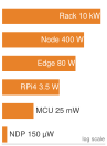
Deployment power spans nearly eight orders, µW to kW.

Henderson, Peter, Jieru Hu, Joshua Romoff, Emma Brunskill, Dan Jurafsky, and Joelle Pineau. 2020. “Towards the Systematic Reporting of the Energy and Carbon Footprints of Machine Learning.” CoRR abs/2002.05651 (248): 1–43. https://doi.org/10.48550/arxiv.2002.05651.

However, measuring power consumption in machine learning systems presents challenges distinct from measuring time or throughput. Power varies with temperature, workload phase, and system configuration in ways that performance metrics do not. Table 14 quantifies how energy demands of ML models vary dramatically across deployment environments, spanning multiple orders of magnitude from TinyML devices consuming mere microwatts to data center racks requiring kilowatts. This wide spectrum illustrates the central challenge in creating standardized benchmarking methodologies (Henderson et al. 2020).

Table 14: Power Consumption Spectrum: The representative deployment points listed here span nearly eight orders of magnitude in power demands, from microwatt-scale TinyML devices (150 µW) to kilowatt-scale ML server racks (10 kW); figure 6 extends the same picture down to 5.6 µW at the TinyML floor and up to roughly 498 kW at the training-cluster ceiling, covering nearly eleven orders of magnitude. This enormous range explains why no single measurement technique or efficiency metric applies universally: benchmarking a 150 µW neural processor requires fundamentally different instrumentation than measuring a 10 kW server rack.

Category	Device Type	Power Consumption
Tiny	Neural Decision Processor (NDP)	150 µW
Tiny	M7 Microcontroller	25 mW
Mobile	Raspberry Pi 4	3.5 W
Mobile	Smartphone	4 W
Edge	Smart Camera	10–15 W
Edge	Edge Server	65–95 W
Cloud	ML Server Node	300–500 W
Cloud	ML Server Rack	4–10 kW

This range spans nearly eight orders and requires scale-specific measurement: microwatt-level TinyML demands different instrumentation than kilowatt-scale racks. A comprehensive framework must maintain consistency, fairness, and reproducibility across both.

Power measurement boundaries

Addressing these measurement challenges requires understanding how power consumption is measured at different system scales, from TinyML devices to full-scale data center inference nodes. Figure 7 lays out the distinct measurement boundaries for each scenario: components in green fall inside the energy accounting boundary, while components with red dashed outlines are explicitly excluded from power measurements. This distinction matters because where the boundary is drawn determines what counts as “efficient.”

\begin{tikzpicture}[font=\footnotesize\sffamily]
\tikzset{%
Line/.style={line width=1.0pt,black!50,text=black,align=center},
BoxG/.style={inner xsep=4pt,
    node distance=0.3,
    draw=GreenLine,
    line width=0.5pt,
    fill=GreenL!60,
    align=flush center,
    rounded corners=2pt,
    minimum height=7.5mm
  },
BoxFill/.style={draw=BackLine,inner xsep=2mm,inner ysep=2mm,
yshift=0mm,fill=BackColor!60,line width=1pt},
BoxFill2/.style={draw=BackLine,inner sep=1pt,fill=BackColor!60,line width=1pt,align=flush center},
BoxDash2/.style={draw=RedLine,inner sep=1pt,fill=white,line width=1pt,dashed,align=flush center},
BoxDash/.style={draw=RedLine,inner xsep=2mm,inner ysep=2mm,
yshift=0mm,fill=white,line width=1pt,dashed,align=flush center},
BoxB/.style={BoxG,fill=cyan!10},
BoxR/.style={BoxG,fill=magenta!15},
BoxO/.style={BoxG,fill=orange!15},
BoxV/.style={BoxG,fill=violet!15}
}
%%%Tiny Example
\foreach \j in {1,2} {
\node[BoxG](1C\j) at({0}, {-0.15*\j}){Compute Unit};
}
\node[BoxB,below =0.4 of  1C2.south west,minimum height=11mm](1C3){Basic\\ Switch};
\node[BoxR,below =0.4 of 1C2.south east,minimum height=11mm](1C4){On Chip\\ SRAM};
\scoped[on background layer]
\node[BoxFill,inner xsep=5mm,fit=(1C1)(1C3)(1C4)](BB1){};
\node[above=4pt of  BB1.north,inner sep=0pt, anchor=south](THE){\textbf{Tiny Example}};
\node[below=4pt of  BB1.south,inner sep=0pt, anchor=north]{Traditional (ultra) Low Power SoC};
%%%Diagam Key
\node[BoxFill,below =1.4 of BB1.219,minimum width=5mm](PMB){};
\node[right=1mm of PMB,yshift=-1pt](PMBT){Power Measurement Boundary};
\node[BoxDash,below =0.13of PMB,,minimum width=5mm](NIB){};
\node[right=1mm of NIB,yshift=-1pt](NIBT){Not in Boundary};
\scoped[on background layer]
\node[BoxFill,fill=white,inner ysep=4mm,yshift=2mm,fit=(PMB)(PMBT)(NIB)](1BB1){};
\node[below left=4pt and -4ptof  1BB1.north west,inner sep=0pt, anchor=north west]{\textbf{Diagram Key}};
%%%Inference Example
%%Typical Inference SoC 1
\foreach \j in {1,2} {
\node[BoxG,minimum height=12mm,yshift=-8mm](2C\j) at({5.6}, {-0.15*\j}){Compute\\ Unit};
}
\node[BoxB,below=of 2C2.south west,anchor=north west,minimum height=12mm](2C3){On Chip\\SRAM};
\node[BoxR,right=of 2C1.north east,anchor=north west,minimum height=10mm](2C4){Switching\\NoC};
\coordinate(S1)at($(2C3.north east)+(1,-0.25)$);
\begin{scope}[local bounding box=CU2,shift={($(S1)+(0,0)$)}]
\foreach \j in {1,2} {
\node[BoxG,minimum height=10mm](22C\j) at({0.15*\j}, {0}){Compute\\ Unit};
}
\end{scope}
\scoped[on background layer]
\node[BoxFill,fill=white,fit=(2C1)(2C3)(2C4)(CU2)](2BB1){};
\node[above left=2pt and -4pt of  2BB1.north west,inner sep=0pt, anchor=south west](TIS){Typical Inference SoC 1};
\node[BoxO,xshift=2mm,below=0mm of 2BB1.east,rotate=90,minimum height=6mm](OCD1){Off-Chip DRAM};
\node[BoxO,xshift=-2mm,above=0mm of 2BB1.west,rotate=90,minimum height=6mm](OCD2){Off-Chip DRAM};
\node[BoxO,below =11mm of OCD2.west,minimum height=8mm,minimum width=6mm](OCD4){};
\node[BoxO,below =11mm of OCD1.west,minimum height=8mm,minimum width=6mm](OCD3){};
%
\path[red](OCD4)-|coordinate(S2)(2C3.south west);
\path[red](OCD3)-|coordinate(S3)(22C2.south east);
\node[BoxG,anchor=west,minimum height=6mm,minimum width=6mm](2B1)at(S2){};
\node[BoxR,anchor=east,minimum height=6mm,minimum width=6mm](2B4)at(S3){};
\node[BoxB,minimum height=6mm,minimum width=6mm](2B3)at($(2B1)!0.66!(2B4)$){};
\node[BoxO,minimum height=6mm,minimum width=6mm](2B2)at($(2B1)!0.33!(2B4)$){};
\scoped[on background layer]
\node[BoxFill,inner xsep=5mm,fit=(OCD3)(TIS)(OCD4)](BB2){};
\scoped[on background layer]
\node[BoxFill,fill=white,fit=(2B1)(2B4),inner ysep=1.5mm,](2BB2){};
\node[above left=2pt and -4pt of  2BB2.north west,inner sep=0pt, anchor=south west]{Typical Inference SoC n};
\scoped[on background layer]
\node[BoxFill,fill=white,fit=(2C1)(2C3)(2C4)(CU2)](2BB1){};
%%%Typical Inference Node 1
\begin{scope}[local bounding box=CU3,shift={($(15,-0.45)+(0,0)$)}]
\foreach \j in {1,2} {
\node[BoxG,minimum height=17mm](3C\j) at({0}, {-0.2*\j}){Accelerator (s) +\\ Local RAM};
}
\node[BoxV,below=4mm of 3C2.south east,minimum width=15mm,minimum height=9mm,anchor=north east](3C3){Active\\ Cooling};
\node[BoxR,below=4mm of 3C3.south east,minimum width=15mm,minimum height=11mm,anchor=north east](3C4){NIC};
\node[BoxR,left=4mm of 3C2.south west,minimum width=15mm,minimum height=9mm,anchor=south east](3C5){Local\\ Storage};
\node[BoxO,below=4mm of 3C2.south west,minimum width=15mm,minimum height=15mm,anchor=north east](3C6){Host\\ DRAM};
\coordinate(S4)at($(3C6.230)+(0,-0.75)$);
\begin{scope}[local bounding box=CU2,shift={($(S4)+(0,0)$)}]
\foreach \j in {1,2} {
\node[BoxG,minimum width=16mm,minimum height=9mm](33C\j) at({0.15*\j}, {0}){Host (s)};
}
\end{scope}
%
\scoped[on background layer]
\node[BoxFill,inner xsep=5mm,fit=(3C1)(3C4)(33C2)](BB4){};
\node[below=4pt of  BB4.south west,inner sep=0pt, anchor=north west]{Traditional Inference Node 1};
\end{scope}
%%%Training Example
\def\ra{1.89mm}
\node[BoxFill2,right=24mm of 3C1.north east,minimum width=41mm,minimum height=6mm,anchor=north west](4C1){
Compute Node 1 (Measured)};
\node[BoxFill2,below=\ra of 4C1.south,minimum width=41mm,minimum height=6mm,anchor=north](4C2){
Compute Node 2 (Measured)};
\node[BoxFill2,below=\ra of 4C2.south,minimum width=41mm,minimum height=9mm,anchor=north](4C3){
Network Switches\\ (Measured/Estimated)};
\node[BoxDash2,below=\ra of 4C3.south,minimum width=41mm,minimum height=6mm,anchor=north](4C4){
Storage Node};
\node[BoxFill2,below=\ra of 4C4.south,minimum width=41mm,minimum height=6mm,anchor=north](4C5){
Compute Node n (Measured)};
\node[BoxDash2,below=\ra of 4C5.south,minimum width=41mm,minimum height=6mm,anchor=north](4C6){
DC Cooling Components};
%
\scoped[on background layer]
\node[BoxFill,inner xsep=5mm,fit=(4C1)(4C6),fill=white,draw=BrownLine,line width=0.75pt](BB6){};
\node[below=4pt of  BB6.south west,inner sep=0pt, anchor=north west]{Training Rack 1};
%%%Right
\node[BoxFill2,right=22mm of 4C1.east,minimum width=7mm,minimum height=6mm,anchor=west](5C1){};
\node[BoxFill2,below=\ra of 5C1.south,minimum width=7mm,minimum height=6mm,anchor=north](5C2){};
\node[BoxFill2,below=\ra of 5C2.south,minimum width=7mm,minimum height=9mm,anchor=north](5C3){};
\node[BoxDash2,below=\ra of 5C3.south,minimum width=7mm,minimum height=6mm,anchor=north](5C4){};
\node[BoxFill2,below=\ra of 5C4.south,minimum width=7mm,minimum height=6mm,anchor=north](5C5){};
\node[BoxDash2,below=\ra of 5C5.south,minimum width=7mm,minimum height=6mm,anchor=north](5C6){};
%
\scoped[on background layer]
\node[BoxFill,inner xsep=4.5mm,fit=(5C1)(5C6),fill=white,draw=BrownLine,line width=0.75pt](BB7){};
\node[below=4pt of  BB7.south west,inner sep=0pt, anchor=north west]{Training Rack n};
%
\node[BoxDash2,rotate=90,minimum height=6mm,minimum width=46mm](RS1)at($(BB2.east)!0.5!(BB4.west)$){Remote Storage};
\node[BoxDash2,rotate=90,minimum height=6mm,minimum width=46mm](RS2)at($(BB4.east)!0.5!(BB6.west)$){Remote Storage};
\node[BoxFill2,rotate=90,minimum height=6mm,minimum width=46mm,
fill=OrangeL!40](RS3)at($(BB6.east)!0.5!(BB7.west)$){Interconnection Fabrics};
\path[red](THE)-|coordinate(S6)(RS1);
\path[red](THE)-|coordinate(S7)($(BB6.north west)!0.5!(BB7.north east)$);
\node[]at(S6){\textbf{Inference Example}};
\node[]at(S7){\textbf{Training Example}};
\end{tikzpicture}

Figure 7: Power Measurement Boundaries: MLPerf defines system boundaries for power measurement, ranging from single-chip devices to full data center nodes, to enable fair comparisons of energy efficiency across diverse hardware platforms. These boundaries delineate which components’ power consumption is included in reported metrics, impacting the interpretation of performance results. Source: (Tschand et al. 2024).

Figure 7 is organized into three categories, Tiny, Inference, and Training examples, each reflecting different measurement scopes based on system architecture and deployment environment. In TinyML systems, the entire low-power SoC, including compute, memory, and basic interconnects, typically falls within the measurement boundary. Inference nodes introduce more complexity, incorporating multiple SoCs, local storage, accelerators, and memory, while often excluding remote storage and off-chip components. Training deployments span multiple racks, where only selected elements, including compute nodes and network switches, are measured, while storage systems, cooling infrastructure, and parts of the interconnect fabric are often excluded.

The measurement boundary determines which energy is counted; workload composition determines where that energy is spent. TensorFlow Mobile measurements attribute 57.3 percent of inference energy to data movement (Boroumand et al. 2018), showing why component-only measurements and raw operation counts can miss the dominant system cost. The next example therefore decomposes MobileNetV2 energy into arithmetic and memory access.

Boroumand, Amirali, Saugata Ghose, Youngsok Kim, Rachata Ausavarungnirun, Eric Shiu, Rahul Thakur, Daehyun Kim, et al. 2018. “Google Workloads for Consumer Devices: Mitigating Data Movement Bottlenecks.” Proceedings of the Twenty-Third International Conference on Architectural Support for Programming Languages and Operating Systems, ASPLOS ’18, 316–31. https://doi.org/10.1145/3173162.3173177.

Napkin Math 1.5: Why INT8 saves energy

Problem: Under the stated 45 nm component-energy model, how much does replacing FP32 with INT8 reduce MobileNetV2 weight-read and arithmetic energy?

Recall from Hardware Acceleration that moving data costs far more energy than computing on it (the energy-movement invariant formalized in Data Engineering and quantified by Horowitz’s energy estimates (Horowitz 2014)). Understanding why quantization reduces energy consumption requires decomposing energy into its physical sources. Two dominant factors determine inference energy: compute operations and memory access.

Narrower datatypes generally require less switching and storage energy per operation, so table 15 reveals an 18× gap between FP32 and INT8 multiply cost:

Table 15: Per-Operation Energy by Precision: Energy cost of a single multiply at FP32, FP16, and INT8, with relative cost normalized to FP32, illustrating why narrower datatypes reduce arithmetic energy. Values follow the 45 nm estimates in Horowitz (2014) and Numbers to Know.

Precision	Multiplier Energy	Relative Cost
FP32	~3.7 pJ/FLOP	1×
FP16	~1.1 pJ/FLOP	0.3×
INT8	~0.2 pJ/FLOP	0.05×

An 8-bit multiplier uses ~18× less energy than a 32-bit floating-point multiplier in this 45 nm component model because narrower arithmetic reduces switching and storage work (Horowitz 2014). Numbers to Know catalogs the per-operation estimates behind these ratios; absolute values and ratios vary with circuit design and process technology.

Table 16 extends the picture to memory access, with energy cost per byte across each tier of the hierarchy:

Table 16: Memory Access Energy by Tier: Per-byte energy cost across the register-to-DRAM hierarchy, with relative cost normalized to a register read, exposing why off-chip memory traffic dominates inference energy budgets. Values follow the same canonical energy-estimate model used in Horowitz (2014) and Numbers to Know.

Memory Level	Energy per Byte	Relative Cost
Register	~0.1 pJ/byte	1×
L1 Cache	~1 pJ/byte	10×
L2 Cache	~5 pJ/byte	50×
DRAM	~160 pJ/byte	1,600×

Memory access dominates: reading one byte from DRAM costs over 1,600× more energy than a register access.

Math: Component energy follows \(E_{\text{load}}=\text{model bytes}\times\text{DRAM energy per byte}\) and \(E_{\text{compute}}=\text{FLOPs}\times\text{operation energy}\). The FP32 terms sum as 2243 µJ + 2,220 µJ = 4,463 µJ; the INT8 terms sum as 561 µJ + 120 µJ = 681 µJ. Dividing the totals gives a 6.6× reduction under this simplified model.

Table 17 combines the two effects in a deliberately simplified MobileNetV2 model. It counts one DRAM read per weight and charges every cataloged FLOP at the listed multiplier energy, while excluding activation traffic, cache behavior, additions as a distinct cost, control overhead, and static power:

Table 17: MobileNetV2 INT8 Simplified Energy Estimate: One weight read plus a multiplier-energy charge for every cataloged FLOP under a 45 nm component-energy model. This is not a whole-device inference measurement.

Component	FP32 (14 MB)	INT8 (3.5 MB)	Savings
One weight read from DRAM	2243 µJ	561 µJ	4×
Compute (600 MFLOP)	2,220 µJ	120 µJ	18.5×
Total	4,463 µJ	681 µJ	6.6×

Systems insight: Within this simplified model, the weight read and the arithmetic contribute comparable FP32 energy (2243 µJ and 2,220 µJ), and INT8 reduces both, taking the total from 4,463 µJ to 681 µJ. This explains the physical mechanism behind potential savings, but battery-life or per-inference claims require controlled whole-device power measurements.

Horowitz, Mark. 2014. “1.1 Computing’s Energy Problem (and What We Can Do about It).” 2014 IEEE International Solid-State Circuits Conference Digest of Technical Papers (ISSCC), 10–14. https://doi.org/10.1109/isscc.2014.6757323.

Shared infrastructure presents additional challenges. In data centers, resources such as cooling systems and power delivery are shared across workloads, complicating attribution of energy use to specific ML tasks. Cooling alone can account for 20–30 percent of total facility power consumption, making it a major factor in energy efficiency assessments (Barroso et al. 2019). Even at the edge, components like memory and I/O interfaces may serve both ML and non-ML functions, further blurring measurement boundaries.

Within a Transformer forward pass, compute intensity and power can vary across kernels. Feed-forward layers commonly use dense matrix multiplications, while attention can be compute- or memory-bound depending on prefill versus decode, sequence and batch shape, and kernel implementation. Dynamic voltage and frequency scaling (DVFS) can further change power with workload demand (Kim et al. 2008). Power benchmarks therefore need sampling and integration windows that capture kernel-level variation rather than inferring whole-model energy from a single instantaneous reading.

Kim, Wonyoung, Meeta S. Gupta, Gu-Yeon Wei, and David Brooks. 2008. “System Level Analysis of Fast, Per-Core DVFS Using on-Chip Switching Regulators.” IEEE International Symposium on High-Performance Computer Architecture (HPCA), HPCA ’08, 123–34. https://doi.org/10.1109/hpca.2008.4658633.

Barroso, Luiz André, Urs Hölzle, and Parthasarathy Ranganathan. 2019. The Datacenter as a Computer: Designing Warehouse-Scale Machines. Synthesis Lectures on Computer Architecture. Springer International Publishing. https://doi.org/10.1007/978-3-031-01761-2.

Support infrastructure, especially cooling, is a major component of energy consumption in large-scale deployments. Data centers must maintain operational temperatures, typically between 20–25 °C, to ensure system reliability. Cooling overhead is captured in the power usage effectiveness metric, which ranges from 1.1 in highly efficient facilities to over 2.0 in less optimized ones (Barroso et al. 2019). The interaction between compute workloads and cooling infrastructure creates complex dependencies; for example, power management techniques like DVFS not only reduce direct processor power consumption but also decrease heat generation, creating cascading effects on cooling requirements. Even edge devices require basic thermal management.

Computational efficiency vs. power consumption

The relationship between computational performance and energy efficiency is a central trade-off in modern ML system design. Historically, computations per kilowatt-hour doubled about every 1.5 years, documenting rapid long-run gains in computing efficiency (Koomey et al. 2011). Processor frequency scaling, however, exposes a local trade-off: higher frequency often requires higher voltage, so dynamic power can rise faster than delivered throughput, reflecting the voltage-frequency-power relationship that underlies DVFS and its diminishing returns (Le Sueur and Heiser 2010).

Koomey, Jonathan, Stephen Berard, Marla Sanchez, and Henry Wong. 2011. “Implications of Historical Trends in the Electrical Efficiency of Computing.” IEEE Annals of the History of Computing 33 (3): 46–54. https://doi.org/10.1109/mahc.2010.28.

Le Sueur, Etienne, and Gernot Heiser. 2010. “Dynamic Voltage and Frequency Scaling: The Laws of Diminishing Returns.” Proceedings of the 2010 International Conference on Power Aware Computing and Systems, 1–8.

Wu, Hao, Patrick Judd, Xiaojie Zhang, Mikhail Isaev, and Paulius Micikevicius. 2020. “Integer Quantization for Deep Learning Inference: Principles and Empirical Evaluation.” arXiv Preprint arXiv:2004.09602 abs/2004.09602.

Gholami, Amir, Sehoon Kim, Zhen Dong, Zhewei Yao, Michael W. Mahoney, and Kurt Keutzer. 2021. “A Survey of Quantization Methods for Efficient Neural Network Inference.” arXiv Preprint arXiv:2103.13630 abs/2103.13630.

In deployment scenarios with strict energy constraints, particularly battery-powered edge devices and mobile applications, optimizing this performance-energy trade-off becomes essential for practical viability. Model optimization techniques offer promising approaches to achieve better efficiency without material accuracy degradation. Numerical precision optimization techniques, which reduce computational requirements while maintaining model quality, demonstrate this trade-off effectively. Integer quantization studies show that reduced-precision computation can often preserve model quality while improving inference speed, memory traffic, and energy efficiency, although the realized gain depends on model, calibration method, and hardware support (Jacob et al. 2018; Wu et al. 2020; Gholami et al. 2021).

Optimization strategies span three interconnected dimensions: accuracy, computational performance, and energy efficiency. Advanced optimization methods enable fine-tuned control over this trade-off space. Similarly, model optimization and compression techniques require careful balancing of accuracy losses against efficiency gains. The optimal operating point among these factors depends heavily on deployment requirements and constraints; mobile applications typically prioritize energy efficiency to extend battery life, while cloud-based services might optimize for accuracy even at higher power consumption costs, benefiting from economies of scale and dedicated cooling infrastructure.

Energy efficiency metrics now occupy a central position in AI system evaluation. Power measurement standards such as MLPerf Power (Tschand et al. 2024) provide standardized frameworks for comparing energy efficiency across hardware platforms and deployment scenarios. These standards enable engineers to systematically balance performance, power consumption, and environmental impact when selecting hardware and optimization strategies.

Standardized power measurement

Power measurement techniques like SPEC Power have long served general computing (Lange 2009), but ML workloads expose a fundamental difficulty: instantaneous power consumption during a single inference can shift rapidly between compute-intensive matrix multiplication and memory-stall phases. MLPerf Power formalizes this problem for ML systems by specifying measurement boundaries, instrumentation, and reporting rules across a wide power range (Tschand et al. 2024). This volatility means that any single-point measurement is misleading, and the act of measurement itself (instrumentation overhead, sampling-induced delays) can perturb the very power profile being characterized.

The core challenge is therefore temporal: characterizing a quantity that fluctuates faster than many measurement instruments can sample. Dense matrix operations in transformer layers create short, intense power spikes that require high-frequency sampling to capture accurately, while CNN inference tends toward more consistent power draw amenable to lower sampling rates. The measurement window must also account for ML-specific warm-up periods, where initial inferences consume more power due to cache population and pipeline initialization. Sliding-window averages over repeated inferences smooth these fluctuations into actionable efficiency numbers, but the window size itself becomes a design parameter that can hide or reveal different aspects of the power profile.

Memory access patterns compound the measurement problem because ML systems often spend more energy moving data than computing on it. Recommendation models like DLRM, for example, can consume more energy on memory access than computation—a pattern that traditional compute-focused power measurement misses entirely. Capturing both compute and memory subsystem power consumption requires instrumenting the full data path, not just the processor.

Heterogeneous accelerator configurations introduce further complexity. GPUs, TPUs, and NPUs each maintain independent power management schemes, and modern SoCs dynamically switch between compute resources based on workload characteristics. Accurate system-level measurement requires synchronized power capture across all active compute units—a challenge that scales with system size. Multi-GPU configurations must account for gradient synchronization energy alongside computation, and multi-node deployments add nontrivial network infrastructure power. At the other extreme, edge deployments must capture the energy cost of model updates and data preprocessing alongside inference itself.

Batch size creates a nonlinear relationship with power consumption that single-point measurements cannot characterize. Larger batches improve compute efficiency (better amortization of memory loads) but increase memory pressure and peak power requirements, meaning the most efficient batch size for throughput may differ from the most efficient batch size for energy. Measurement across multiple batch sizes is essential for a complete efficiency profile. System idle states deserve equal attention, particularly for intermittent edge workloads: a wake-word detection TinyML system that actively processes audio for only a small fraction of operating time may be dominated by idle power consumption rather than inference energy. Finally, sustained ML workloads can cause temperature increases that trigger thermal throttling and alter power consumption patterns—an effect particularly acute in edge devices, where thermal constraints limit sustained performance and make extended benchmarking runs essential for realistic characterization.

MLPerf power case study

MLPerf Power (Tschand et al. 2024) turns power measurement from a device-specific reading into a comparable efficiency claim: how many useful inferences a system delivers per watt under a defined boundary. The methodology applies standardized evaluation principles across data center, edge, and tiny inference settings, where the relevant decision changes from rack operating cost to battery life to microwatt-scale endurance.

Boundary-aware standardization matters because the same hardware family can look efficient or wasteful depending on boundary and workload. By adapting the protocol to CPUs, accelerators, and heterogeneous systems while preserving measurement integrity, MLPerf Power makes cross-platform comparisons meaningful across different computing scales.

The benchmark has accumulated many reproducible measurements submitted by industry organizations, demonstrating submitted hardware capabilities and the sector-wide focus on energy-efficient AI technology. The data-center panel in figure 8 shows how normalized energy efficiency has evolved across successive MLPerf Inference versions. The gains differ by workload and start version: RetinaNet and ResNet show the largest plotted increases, while GPT-J, DLRM-v2, and Llama 2 cover fewer benchmark rounds, making their gains less directly comparable.

Figure 8: Data-Center Energy Efficiency Gains: Each series is normalized to its own first plotted version, so compare improvement within a workload rather than absolute efficiency across workloads. Source: (Tschand et al. 2024).

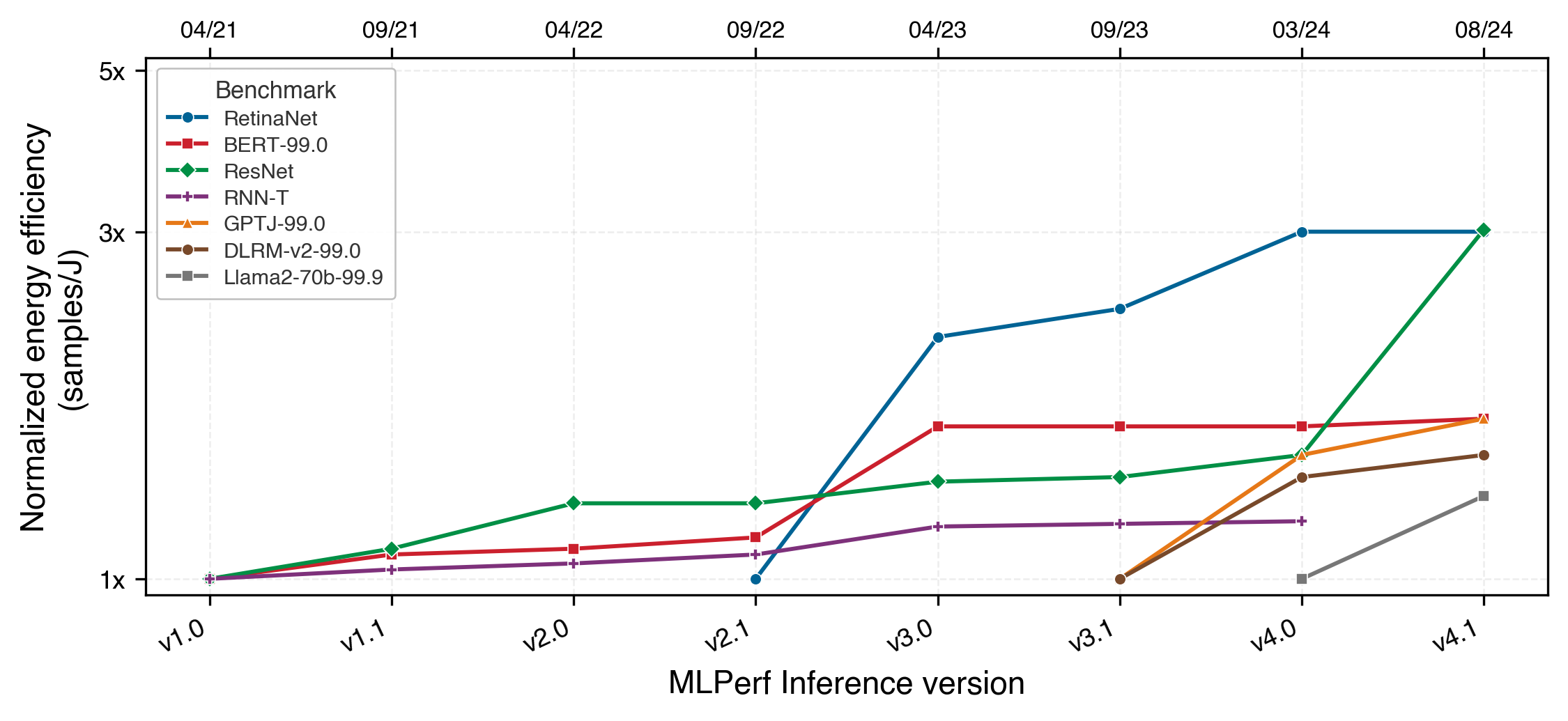
Tschand, Arya, Arun Tejusve Raghunath Rajan, Sachin Idgunji, Anirban Ghosh, Jeremy Holleman, Csaba Kiraly, Pawan Ambalkar, et al. 2024. “MLPerf Power: Benchmarking the Energy Efficiency of Machine Learning Systems from \(\mu\)Watts to MWatts for Sustainable AI.” 2025 IEEE International Symposium on High Performance Computer Architecture (HPCA), 1201–16. https://doi.org/10.1109/hpca61900.2025.00092.

RetinaNet and ResNet show the largest plotted gains, each reaching 3\(\times\) its initial normalized efficiency. BERT and GPT-J reach about 1.9\(\times\), while DLRM-v2 reaches about 1.7\(\times\), Llama 2 about 1.5\(\times\), and RNN-T about 1.3\(\times\).

Timing protocols and power instrumentation provide the raw data for benchmarking. Raw data alone, however, does not guarantee sound conclusions. Converting measurements into meaningful comparisons requires understanding the systematic sources of error, bias, and misalignment that can make even carefully collected benchmark numbers misleading.

Self-Check: Question

1. A vendor advertises an AI accelerator as delivering ‘\(10\text{ TOPS}\) at \(0.5\text{ W}\).’ When deployed in a production server, the total power consumption measured at the wall socket increases by \(4.5\text{ W}\) for that same workload. What explains this discrepancy in benchmarking methodology?

   1. The vendor drew an isolated power measurement boundary around the compute core silicon only, omitting DRAM interfaces, PCIe host transfers, voltage regulators, CPU preprocessing, and cooling fans
   2. The electrical wall outlet was defective and provided improper alternating current
   3. Power consumption in digital circuits is inherently non-deterministic and varies by \(10\times\) between runs
   4. The vendor measured power during sleep mode rather than active compute

2. An accelerator increases its operating clock frequency to achieve a \(5\%\) increase in inference throughput, but this requires increasing the supply voltage by \(15\%\). Because dynamic power scales as \(P \propto V^2 f\), active power consumption increases by approximately \(39\%\). What is the systems consequence of this operating point for a power-constrained edge deployment?

   1. It is an optimal trade-off because throughput is always the only metric that matters
   2. It represents a severe energy efficiency regression, reducing performance-per-watt by roughly \(24\%\) and accelerating battery drain and thermal throttling
   3. Performance-per-watt increases because higher frequency reduces static leakage
   4. The device will operate cooler because inferences finish \(5\%\) sooner

3. Explain why instantaneous power sampling during an ML inference workload produces misleading results, and describe how standardized protocols calculate total energy.

4. True or False: In standardized ML power benchmarking, measuring the power draw of the arithmetic compute units (ALUs and tensor cores) is sufficient because the energy required to read and write data from DRAM is negligible in comparison.

5. Order the following steps in a standardized MLPerf Power measurement protocol from start to finish:

1. Integrate instantaneous power readings over the full run duration (\(E = \int P(t) \, dt\)) and compute Joules per inference
2. Establish the physical measurement boundary and connect a calibrated power analyzer in series with the system power supply
3. Execute unmeasured warm-up iterations until the device achieves thermal equilibrium (steady-state junction temperature)
4. Measure and record the baseline idle/quiescent power consumption while the system is waiting for requests
5. Execute the synchronized inference benchmark workload while logging continuous high-frequency time-series power and temperature data

See Answers →

Benchmarking Best Practices

An inference stack that passes a steady-state lab run can still miss latency targets when production traffic arrives in bursts, or when the input mix shifts toward expensive examples. Training throughput, inference latency, and power efficiency each have established measurement protocols validated through MLPerf, but knowing what to measure is insufficient without understanding what benchmarks cannot capture and why this gap has derailed countless deployments.

Benchmarks make simplifying assumptions that enable standardized comparison but can diverge from production reality. Training suites may freeze datasets and tightly specify randomness; production data and retraining conditions evolve. Inference suites often emphasize a defined steady-state scenario; production traffic can be bursty and time-varying. Power benchmarks control thermal conditions; deployed hardware may encounter different ambient temperatures and sustained-load behavior. Four categories of limitations (statistical, deployment-related, system design, and organizational) determine whether benchmark results translate to deployment success.

Statistical and methodological issues

Benchmark results are only as reliable as the measurements that produce them. Three pervasive issues undermine this reliability if left unaddressed.

Incomplete problem coverage represents one of the most pervasive limitations. Many benchmarks, while useful for controlled comparisons, fail to capture the full diversity of real-world applications. Common image classification datasets such as CIFAR-10 (Krizhevsky 2009) contain a limited variety of images. Models that perform well on these datasets may struggle when applied to more complex, real-world scenarios with greater variability in lighting, perspective, and object composition. This gap between benchmark tasks and real-world complexity means strong benchmark performance provides limited guarantees about practical deployment success.

Krizhevsky, Alex. 2009. Learning Multiple Layers of Features from Tiny Images. University of Toronto.

Statistical insignificance arises when benchmark evaluations are conducted on too few data samples or trials, and it is most acute in settings where the evaluation medium itself introduces variance. Large language model evaluation exemplifies this problem: whether scoring a new LLM against a reference using human preference ratings or an LLM-as-judge protocol, the evaluation signal carries high variance because judges respond differently to prompt phrasing, ordering effects, and response length. A reported two-point preference win can disappear entirely across a different judge configuration or prompt template. Rigorous LLM benchmarking therefore requires statistical methods—bootstrap confidence intervals or paired significance tests—applied across enough prompts and response pairings to separate a genuine capability improvement from evaluation noise. Without sufficient trials and diverse input distributions, benchmarking results will mislead: reported differences reflect evaluation noise rather than genuine capability. The statistical confidence intervals around benchmark scores often go unreported, obscuring whether measured differences represent genuine improvements or measurement noise.

Reproducibility represents a major ongoing challenge. Benchmark results can vary measurably depending on factors such as hardware configurations, software versions, and system dependencies. Small differences in compilers, numerical precision, or library updates can lead to inconsistent performance measurements across different environments. To mitigate this issue, MLPerf addresses reproducibility by providing reference implementations, standardized workloads and run rules, and strict submission guidelines. Even with these efforts, achieving true consistency across diverse hardware platforms remains an ongoing challenge. The proliferation of optimization libraries, framework versions, and compiler flags creates a vast configuration space where slight variations produce different results.

Laboratory-to-deployment performance gaps

Statistical rigor ensures that benchmark measurements are accurate. Accurate measurements of the wrong thing, however, still lead to deployment failures. Benchmarks must also align with practical deployment objectives.

Misalignment with real-world goals occurs when benchmarks emphasize metrics such as speed, accuracy, and throughput, while practical AI deployments require balancing multiple objectives including power efficiency, cost, and robustness. A model that achieves top-line accuracy on a benchmark may be impractical for deployment if it consumes excessive energy or requires expensive hardware. Similarly, optimizing for average-case performance on benchmark datasets may neglect tail-latency requirements that determine user experience in production systems. The multi-objective nature of real deployment, encompassing resource constraints, operational costs, maintenance complexity, and business requirements, extends far beyond the single-metric optimization that most benchmarks reward.

System design challenges

Statistical methodology and deployment alignment address how performance is measured and what is optimized. A third category of limitations emerges from the physical systems being measured. Hardware behavior depends on environmental conditions, architectural compatibility, and operational context in ways that complicate fair comparison.

Environmental conditions affect benchmarks in measurable ways. Benchmark results depend on physical conditions (ambient temperature, humidity, altitude) and operational context (background processes, network load, power supply stability) in subtle but measurable ways. Elevated temperatures trigger thermal throttling that reduces computational speed; background processes compete for resources and alter performance characteristics. Ensuring valid benchmarks requires controlling these factors to the extent possible (temperature-controlled environments, standardized system states, documented background loads) and, when full control is impractical (as in distributed or cloud-based benchmarking), detailed reporting of conditions so that others can account for potential variations when interpreting results.

The hardware lottery³⁴ (Hooker 2021) presents another critical issue. The success of a machine learning model is often dictated not only by its architecture and training data but also by how well it aligns with the underlying hardware. Some models perform exceptionally well not because they are inherently superior but because they map naturally onto GPU or TPU parallel processing capabilities. Other promising architectures may be systematically overlooked because they do not fit dominant hardware platforms.

³⁴ Hardware lottery: Coined by Hooker (2021) to describe how algorithmic success depends on alignment with available hardware and software. Transformer workloads benefit from dense matrix operations that map efficiently to modern accelerators, while graph neural networks and sparse mixture-of-experts models can be harder to evaluate when available silicon and software stacks favor dense kernels. Hardware-specific leaderboards therefore favor architectures aligned with the measured platform and may obscure alternatives that would fare differently under other hardware assumptions.

Hooker, Sara. 2021. “The Hardware Lottery.” Communications of the ACM 64 (12): 58–65. https://doi.org/10.1145/3467017.

Hardware compatibility dependence introduces subtle but significant biases into benchmarking results. A model that is highly efficient on a specific GPU may perform poorly on a CPU or a custom AI accelerator. Figure 9 makes this hardware dependence concrete by comparing model performance across different platforms. On the CPU uint8 and GPU configurations, the multi-hardware models track the “MobileNetV3 Large min” baseline closely, reaching roughly 77 percent top-1 ImageNet accuracy where the baseline reaches about 75 percent. On the EdgeTPU and DSP hardware the same multi-hardware models sustain that 77 percent at substantially lower latency, while a model tuned only for the CPU would forfeit those gains. This reveals that the “best” model depends entirely on deployment target: a conclusion impossible to reach from single-platform benchmarks.

\begin{tikzpicture}[font=\small\sffamily]
\pgfplotsset{myaxis/.style={
  /pgf/number format/.cd,
  1000 sep={},
   legend style={at={(1.85,0.97)}, anchor=north},
   legend cell align=left,
   legend style={fill=BrownL!30,draw=BrownLine,row sep=1.1pt,
   font=\fontsize{6pt}{6}\selectfont\sffamily},
   width=58mm,
   height=50mm,
   axis line style={thick,-latex},
   tick label style={/pgf/number format/assume math mode=true},
   yticklabel style={xshift=0mm,font=\fontsize{7pt}{7}\selectfont\sffamily,
   /pgf/number format/.cd, fixed, fixed zerofill, precision=2},
   xticklabel style={font=\fontsize{7pt}{7}\selectfont\sffamily},
   ylabel style={font=\fontsize{7pt}{7}\selectfont\sffamily,align=center,yshift=-1mm},
   xlabel style={font=\fontsize{7pt}{7}\selectfont\sffamily},
   tick style={draw=black!60,thin},
   tick align=outside,
   tick pos=bottom,
   major tick length=1mm,
   title style={yshift=-4pt},
   grid=none,
   major grid style={black!60},
   x tick label style={rotate=0, anchor=north,yshift=2pt},
   ylabel={Top-1 ImageNet Acc},
   cycle list={
     {myblue,mark=*,mark size=1.5pt,line width=1pt},
     {myolive,mark=*,mark size=1.5pt,line width=1pt},
     {mygreen,mark=*,mark size=1.5pt,line width=1pt},
     {myred,mark=*,mark size=1.5pt,line width=1pt},
     {mypurple,mark=*,mark size=1.5pt,line width=1pt},
     {myorange,mark=*,mark size=1.5pt,line width=1pt},
     {black,mark=triangle*,mark size=2.5pt,line width=1pt},
     {mybrown,mark=triangle*,mark size=2.5pt,line width=1pt}
  }
    }}

%LEFT
 \begin{scope}[local bounding box=GR1,shift={(0,0)}]
\begin{axis}[myaxis,
  xmin=7,
  xmax=115,
  xtick={25,50,75,100},
  ymin=0.6912, ymax=0.783,
  ytick={0.70,0.72,...,0.78},
  xlabel={Pixel 4 CPU float latency},
]
%blue
\addplot+[] coordinates {(24.2,0.711)(37.1,0.736)(55,0.752)};
%olive
\addplot+[] coordinates {(18,0.703)(25.3,0.733)(39,0.753)};
%green
\addplot+[] coordinates {(14,0.731)(20.3,0.754)(30.5,0.766)};
%red
\addplot+[] coordinates {(12,0.695)(17.3,0.725)(27,0.748)};
%purple
\addplot+[] coordinates {(48,0.743)(60,0.762)(109.5,0.779)};
%orange
\addplot+[] coordinates {(20.5,0.7245)(28,0.75)(41.5,0.765)};
%black
\addplot+[] coordinates {(20.5,0.7345)(25,0.748)(35.5,0.758)};
%brown
\addplot+[] coordinates {(26,0.748)(31,0.759)(45.5,0.769)};
\coordinate(X)at(axis cs: 20.3,0.754);
\end{axis}
\end{scope}
%above center
\begin{scope}[local bounding box=GR2,shift={(5.7,0)}]
\begin{axis}[myaxis,
  xmin=5.4,
  xmax=34.4,
  xtick={10,20,30},
  ymin=0.691, ymax=0.782,
  ytick={0.70,0.72,...,0.78},
  xlabel={Pixel 4 CPU uint8 latency}
]
%blue
\addplot+[] coordinates {(9.0,0.711)(12.8,0.736)(18.2,0.751)};
%olive
\addplot+[] coordinates {(8.5,0.703)(11.5,0.733)(16.6,0.753)};
%green
\addplot+[] coordinates {(9.5,0.731)(13.3,0.753)(17.9,0.7655)};
%red
\addplot+[] coordinates {(6.8,0.695)(8.7,0.726)(12.6,0.749)};
%purple
\addplot+[] coordinates {(16.1,0.743)(19.5,0.762)(33.0,0.7785)};
%orange
\addplot+[] coordinates {(11.3,0.7245)(14.8,0.749)(20.2,0.765)};
%black
\addplot+[] coordinates {(10.2,0.7345)(11.5,0.749)(14.8,0.758)};
%brown
\addplot+[] coordinates {(12.3,0.748)(13.9,0.758)(18.4,0.769)};
\end{axis}
\end{scope}

%above right
\begin{scope}[local bounding box=GR3,shift={(11.4,0)}]
\begin{axis}[myaxis,
  xticklabel style={xshift=0mm,font=\fontsize{7pt}{7}\selectfont\sffamily,
  /pgf/number format/.cd, fixed, fixed zerofill, precision=1},
  xmin=2.2,
  xmax=12.9,
  xtick={2.5,5.0,7.5,10.0,12.5},
  ymin=0.691, ymax=0.782,
  ytick={0.70,0.72,...,0.78},
  xlabel={Pixel 4 GPU Adreno 640 latency}
]
%blue
\addplot+[] coordinates {(3.7,0.711)(4.8,0.7355)(7.1,0.751)};
%olive
\addplot+[] coordinates {(3.4,0.703)(4.4,0.7323)(5.7,0.7525)};
%green
\addplot+[] coordinates {(4.75,0.731)(5.62,0.753)(7.29,0.7655)};
%red
\addplot+[] coordinates {(2.7,0.695)(3.37,0.725)(4.6,0.748)};
%purple
\addplot+[] coordinates {(6.1,0.7427)(7.5,0.7615)(12.4,0.7781)};
%orange
\addplot+[] coordinates {(4.86,0.7245)(5.9,0.749)(7.82,0.764)};
%black
\addplot+[] coordinates {(3.92,0.7345)(4.4,0.748)(5.58,0.758)};
%brown
\addplot+[] coordinates {(4.73,0.747)(5.39,0.758)(6.64,0.768)};
\end{axis}
\end{scope}
%below left
\begin{scope}[local bounding box=GR4,shift={(0,-5)}]
\begin{axis}[myaxis,
  xticklabel style={xshift=0mm,font=\fontsize{7pt}{7}\selectfont\sffamily,
  /pgf/number format/.cd, fixed, fixed zerofill, precision=1},
  xmin=1.85,
  xmax=3.59,
  xtick={2.0,2.5,3.0,3.5},
  ymin=0.691, ymax=0.782,
  ytick={0.70,0.72,...,0.78},
  xlabel={Pixel 4 EdgeTPU latency}
]
%blue
\addplot+[] coordinates {(1.92,0.711)(2.38,0.7359)(2.845,0.7514)};
%olive
\addplot+[] coordinates {(2.03,0.703)(2.3,0.7325)(2.93,0.7525)};
%green
\addplot+[] coordinates {(1.942,0.6947)(2.105,0.7253)(2.58,0.749)};
%red
\addplot+[] coordinates {(1.942,0.6947)(2.105,0.7253)(2.58,0.749)};
%purple
\addplot+[] coordinates {(2.34,0.7425)(2.67,0.7615)(3.495,0.77844)};
%orange
\addplot+[] coordinates {(2.6,0.7245)(3.09,0.7484)(3.42,0.764)};
%black
\addplot+[] coordinates {(2.08,0.734)(2.21,0.748)(2.44,0.7577)};
%brown
\addplot+[] coordinates {(2.315,0.747)(2.4,0.7575)(2.9,0.7676)};
\end{axis}
\end{scope}
%below right
\begin{scope}[local bounding box=GR5,shift={(5.7,-5)}]
\begin{axis}[myaxis,
  xmin=2.35,
  xmax=6.35,
  xtick={3,4,5,6},
  ymin=0.691, ymax=0.782,
  ytick={0.70,0.72,...,0.78},
  xlabel={Pixel 4 DSP Qualcomm Snapdragon 855 latency}
]
%blue
\addplot+[] coordinates {(2.52,0.711)(3.05,0.736)(3.72,0.751)};
\addlegendentry{MobileNet V1}
%olive
\addplot+[] coordinates {(3.3,0.703)(3.84,0.733)(4.97,0.7525)};
\addlegendentry{MobileNet V2}
%green
\addplot+[] coordinates {(3.95,0.731)(4.5,0.753)(5.15,0.7652)};
\addlegendentry{MobileNet V3 Large}
%red
\addplot+[] coordinates {(2.92,0.6945)(3.29,0.725)(3.81,0.7488)};
\addlegendentry{MobileNet V3 Large min}
%purple
\addplot+[] coordinates {(3.82,0.7425)(4.29,0.7615)(6.14,0.7781)};
\addlegendentry{MobileNet-EdgeTPU}
%orange
\addplot+[] coordinates {(3.54,0.7245)(3.885,0.7485)(5.06,0.764)};
\addlegendentry{ProxylessNAS-Mobile}
%black
\addplot+[] coordinates {(3.08,0.7341)(3.377,0.748)(4.05,0.762)};
\addlegendentry{Multi-MAX}
%brown
\addplot+[] coordinates {(3.6,0.747)(3.84,0.759)(4.52,0.7675)};
\addlegendentry{Multi-AVG}
\coordinate(Y)at(axis cs: 4.5,0.753);
\end{axis}
\end{scope}
\draw[VioletLine!60,-{Triangle[width=8pt,length=13pt]}, line width=3pt,
shorten <=2pt](X)--(Y);
\end{tikzpicture}

Figure 9: Hardware-Dependent Latency–Accuracy Trade-offs: Each panel holds top-1 ImageNet accuracy on the vertical axis while using a target-specific latency scale horizontally. The arrow links MobileNetV3 Large at roughly equal accuracy on CPU float and DSP, exposing the hardware-dependent latency shift. Source: (Chu et al. 2021).

Chu, Grace, Okan Arikan, Gabriel Bender, Weijun Wang, Achille Brighton, Pieter-Jan Kindermans, Hanxiao Liu, Berkin Akin, Suyog Gupta, and Andrew Howard. 2021. “Discovering Multi-Hardware Mobile Models via Architecture Search.” 2021 IEEE/CVF Conference on Computer Vision and Pattern Recognition Workshops (CVPRW), 3016–25. https://doi.org/10.1109/cvprw53098.2021.00337.

Without careful benchmarking across diverse hardware configurations, the field risks favoring architectures that “win” the hardware lottery rather than selecting models based on their intrinsic strengths. This bias can shape research directions, influence funding allocation, and impact the design of next-generation AI systems. In extreme cases, it may even stifle innovation by discouraging exploration of alternative architectures that do not align with current hardware trends.

Organizational and strategic issues

The limitations discussed in this section arise from technical challenges: statistical noise, deployment misalignment, environmental variance, and hardware compatibility. A fourth category emerges from human factors—and these may be the hardest to mitigate because they involve incentives rather than instrumentation. Competitive pressures and research incentives create systematic biases in how benchmarks are used and interpreted. These organizational dynamics require governance mechanisms and community standards to maintain benchmark integrity.

Benchmark engineering

While the hardware lottery is an unintended consequence of hardware trends, benchmark engineering is an intentional practice where models or systems are explicitly optimized to excel on specific benchmark tests. This practice can lead to misleading performance claims and results that do not generalize beyond the benchmarking environment.

Benchmark engineering occurs when AI developers fine-tune hyperparameters, preprocessing techniques, or model architectures specifically to maximize benchmark scores rather than improve real-world performance. The distinction between legitimate optimization and benchmark engineering is often blurry, sitting at the threshold where tuning for a specific benchmark crosses into overfitting to it. For example, an object detection model might be carefully optimized to achieve record-low latency on a benchmark but fail when deployed in dynamic, real-world environments with varying lighting, motion blur, and occlusions. Similarly, a language model might be tuned to excel on benchmark datasets but struggle when processing conversational speech with informal phrasing and code-switching.

The pressure to achieve high benchmark scores is often driven by competition, marketing, and research recognition. Benchmarks are frequently used to rank AI models and systems, creating an incentive to optimize specifically for them. While this can drive technical advancements, it also risks prioritizing benchmark-specific optimizations at the expense of broader generalization—precisely the Goodhart’s Law dynamic introduced in section 1.1 and illustrated with the BLEU-score example in section 1.3.1.

Bias and over-optimization

The practitioner consuming a benchmark result must determine whether a number reflects legitimate optimization or benchmark engineering. Several practices make that distinguishable, and each catches a specific failure at a specific cost. Transparency is the first line of defense: a submission that documents every optimization applied lets a reader separate general improvement from benchmark-specific tuning, at the cost of exposing techniques a vendor may prefer to keep proprietary. Reporting both benchmark and real-world deployment results closes the same gap from the other side. Diversified evaluation across multiple, continuously updated benchmarks raises the cost of overfitting to any single test set, because a model engineered to win one cannot easily win them all; its cost is the engineering effort of maintaining many benchmarks.

Standardization and third-party verification raise the bar further. Independent audits catch results that fail to reproduce across settings, and the existence proof for this mechanism appears two sections later in MLPerf’s reference-vs-submission validation (section 1.10.5), which disqualifies any submission that cannot hit the reference accuracy target. Application-specific testing catches the failure controlled benchmarks structurally cannot: an autonomous-driving model must be exercised across the weather, lighting, and urban settings it will actually meet, not judged solely on a curated dataset. Multi-hardware testing catches the last case, performance that is really hardware-lottery alignment rather than model quality, by confirming that a result does not depend on compatibility with one platform.

Benchmark evolution

A persistent challenge in benchmarking is that benchmarks are rarely static. As AI systems evolve, so must the benchmarks that evaluate them. A performance target that discriminates well under one generation of models, hardware, and applications may lose relevance under another. While benchmarks are essential for tracking progress, they can also become outdated, leading to over-optimization for old metrics rather than real-world performance improvements.

This evolution is evident in the history of AI benchmarks. Early model benchmarks, for instance, focused heavily on image classification and object detection, as these were some of the first widely studied deep learning tasks. However, as AI expanded into natural language processing, recommendation systems, and generative AI, it became clear that these early benchmarks no longer reflected the most important challenges in the field. In response, new benchmarks emerged to measure language understanding (Wang et al. 2018, 2019) and generative AI (Liang et al. 2022).

Wang, Alex, Yada Pruksachatkun, Nikita Nangia, Amanpreet Singh, Julian Michael, Felix Hill, Omer Levy, and Samuel R. Bowman. 2019. “SuperGLUE: A Stickier Benchmark for General-Purpose Language Understanding Systems.” arXiv Preprint arXiv:1905.00537.

Benchmark evolution extends beyond the addition of new tasks to encompass new dimensions of performance measurement. While traditional AI benchmarks emphasized accuracy and throughput, deployed applications demand evaluation across multiple criteria: fairness, robustness, scalability, and energy efficiency. Figure 10 makes these disparate requirements concrete by mapping scientific applications across data rate and computation time. Specifically, Large Hadron Collider sensors must process data at rates approaching \(10^{14}\) bytes per second with nanosecond-scale computation times, while mobile applications operate at \(10^{4}\) bytes per second with longer computational windows—a span of roughly ten orders of magnitude in data rate and six to seven in computation time. This range of requirements necessitates specialized benchmarks. For example, edge AI applications benefit from benchmarks like MLPerf that evaluate performance under resource constraints, and scientific application domains need their own “Fast ML for Science” benchmarks (Duarte et al. 2022).

\scalebox{0.77}{%
\begin{tikzpicture}[font=\small\sffamily]
\pgfplotsset{
  errorplot/.style n args={1}{
    scatter,
    line width=0.75pt,
    only marks,
    mark=none,
    error bars/.cd,
      x dir=both, x explicit,
      y dir=both, y explicit relative,
    error bar style={#1, line width=0.75pt, solid},
    error mark options={line width=0.75pt, mark size=3pt, rotate=90}
  }
}
\begin{axis}[
  ymin=2, ymax=14.3,
  ytick={2,4,6,8,10,12,14},
  yticklabels={10\textsuperscript{2},10\textsuperscript{4},10\textsuperscript{6},
  10\textsuperscript{8},10\textsuperscript{10},10\textsuperscript{12},10\textsuperscript{14}},
  xmin=2, xmax=9.0,
  xtick={2,3,4,5,6,7,8,9},
  xticklabels={10\textsuperscript{-9},10\textsuperscript{-7},10\textsuperscript{-5},
  10\textsuperscript{-3},10\textsuperscript{-1},10\textsuperscript{1},10\textsuperscript{3},10\textsuperscript{5}},
   xlabel={Computation time [s]},
   ylabel={Data rate [bytes/s]},
   width=120mm, height=120mm,
   legend style={at={(0.7,0.3)},anchor=south west},
   grid=both
]
%LHC sensor
\addplot+[errorplot={RedLine}]
  coordinates {(2.6,13.72) +- (0.1,0.022)
}node[RedLine,pos=1,right=8pt,anchor=west]{LHC sensor};
%X-ray diffraction
\addplot+[errorplot={VioletLine}]
  coordinates {(3.82,7.52) +- (0.33,0.069)
 } node[VioletLine,pos=1,right=22pt,anchor=west]{X-ray diffraction};
%Internet-of-things
\addplot+[errorplot={OliveLine}]
   coordinates {(5.49,5.50) +- (0.5,0.18)
} node[OliveLine,pos=1,right=22pt,anchor=west]{Internet of Things};
%Mobile devices
\addplot+[errorplot={cyan!90!black}]
   coordinates {( 5.87,4.23) +- (0.1,0.044)
}node[cyan!90!black,pos=1,right=7pt,anchor=west]{Mobile devices};
%Plasma control
\addplot+[errorplot={green!70!black}]
  coordinates { (4.0,9.51) +- (0.15,0.) [meta=a]
}node[green!70!black,pos=1,above right=12pt,anchor=north west]{Plasma control};
%LHC trigger
\addplot+[errorplot={BrownLine}]
  coordinates { (3.42,9.11) +- (0.42,0.) }
node[BrownLine,pos=1, right=17pt,anchor= west]{LHC trigger};
%Beam control
\addplot+[errorplot={OrangeLine}]
  coordinates { (4.92,4.69) +- (0.42,0.) [meta=c]
}node[OrangeLine,pos=0.1,below=2pt,anchor=north east]{Beam control};
%
\addplot+[line width=1.15pt,
  scatter,
  only marks,mark size=3.25pt,
  scatter src=explicit symbolic,
  scatter/classes={
   a={mark=+,blue}, b={mark=+,red}, c={mark=+,purple},
   d={mark=+,orange!70!black},e={mark=+,violet!60!black},f={mark=+,GreenD}
  }
]
table[meta=label, row sep=crcr]{
  x    y    label \\
  3.49 8.90 a     \\
  3.34 9.89 b     \\
  2.99 9.97 c     \\
  5.00 6.72 d     \\
  4.330 8.73 f\\
  4.50 6.50 e\\
};
\node[blue,below left=2pt and -11pt]at(axis cs:3.49,8.93){DUNE readout};
\node[red,below left=0.5pt and 0pt]at(axis cs:3.34,9.89){EIC trigger};
\node[purple,above right=2.5pt and -19pt]at(axis cs:2.99,9.97){Qubit Readout};
\node[orange!70!black,above right=1.5pt and 1pt]at(axis cs:5.00,6.72){Neuro};
\node[violet!60!black,below left=0.5pt and 0pt]at(axis cs:4.50,6.50 ){Magnet quench};
\node[GreenD,below right=0.5pt and 0pt]at(axis cs:4.330,8.78){Electron microscopy};
%
\coordinate(A)at(axis cs:2,14.3);
\coordinate(B)at(axis cs:5.33,14.3);
\coordinate(C)at(axis cs:5.33,4.69);
\coordinate(D)at(axis cs:2,4.69);
\scoped[on background layer]
\filldraw[cyan!5](A)--(B)--(C)--(D)--cycle;
\node[align=center]at(axis description cs: 0.8,0.92){\textbf{Fast ML for Science}\\benchmark tasks};
\end{axis}
\end{tikzpicture}}

Figure 10: Performance Spectrum: Scientific and edge applications occupy widely separated operating points in data rate and available computation time, motivating benchmarks tied to each application’s timing and data-movement constraints. Source: (Duarte et al. 2022).

Duarte, Javier, Nhan Tran, Ben Hawks, Christian Herwig, Jules Muhizi, Shvetank Prakash, and Vijay Janapa Reddi. 2022. “FastML Science Benchmarks: Accelerating Real-Time Scientific Edge Machine Learning.” arXiv Preprint arXiv:2207.07958.

The need for evolving benchmarks also presents a challenge: stability vs. adaptability. On the one hand, benchmarks must remain stable for long enough to allow meaningful comparisons over time. If benchmarks change too frequently, it becomes difficult to track long-term progress and compare new results with historical performance. On the other hand, failing to update benchmarks leads to stagnation, where models are optimized for outdated tasks rather than advancing the field. Striking the right balance between benchmark longevity and adaptation is an ongoing challenge for the AI community.

Evolving benchmarks remains essential for meaningful progress measurement. Without updates, benchmarks become detached from real-world needs, and researchers optimize for artificial test cases rather than practical challenges. The transition from ImageNet-era accuracy benchmarks to multi-dimensional evaluations spanning fairness, robustness, and energy efficiency illustrates this evolution in practice.

MLPerf synthesis and benchmark gaming

Benchmark gaming begins when a compiler, runtime, or hardware stack optimizes for the benchmark artifact rather than the workload it is supposed to represent. MLPerf counters that risk by synthesizing the principles discussed throughout this chapter into a single evolving framework: reference implementations and strict submission rules enforce reproducibility, deployment-specific suites (Inference, Mobile, Client, Tiny) align with the three-dimensional evaluation framework, and regular task updates (including generative AI and energy-efficient computing) prevent benchmark stagnation. In the Hennessy & Patterson tradition of quantitative systems, benchmarks are targets, not merely passive measurements. The Goodhart dynamic introduced in section 1.1 applies here in full force. In the high-stakes world of AI hardware, it manifests as benchmark gaming: optimizing hardware or compilers specifically for the benchmark’s unique characteristics, rather than for real-world performance.

Three hypothetical shortcuts illustrate the kinds of benchmark-specific behavior that rigorous run rules must forbid:

• Precision dropping: A compiler silently lowers precision only for the benchmark, without disclosing the changed numerical contract.
• Benchmark-specific operator removal: An implementation exploits the evaluation set or quality threshold to skip work that a general deployment must perform.
• Benchmark detection: A system recognizes the benchmark workload and selects a path unavailable to ordinary inputs.

MLPerf constrains this gaming through reference implementations, quality targets, submission rules, and audits. In the Closed Division, preprocessing, postprocessing, and the model must remain equivalent to the reference, while submitters may change frameworks, layouts, kernels, and numerical representation within those rules. Open submissions may substitute or retrain models but are labeled separately. Accuracy is one guardrail; other rules prohibit benchmark detection and input-dependent optimization.

Yet even the most rigorous system benchmarks validate only one dimension of deployment readiness. A system achieving record throughput and efficiency on MLPerf says nothing about whether the model it runs is accurate on real-world inputs, or whether the data it was trained on represents the population it will serve. Hardware that delivers promised TFLOP/s is necessary but insufficient; the model running on that hardware must preserve the quality users depend on, and the data that shaped that model must represent the world it will encounter. Completing the validation stack requires turning from hardware to the model and data dimensions of the three-dimensional framework.

Self-Check: Question

1. An image classification model achieves \(95\%\) accuracy on the CIFAR-10 benchmark test set, but when deployed on a mobile robot operating in a warehouse, its accuracy drops to \(70\%\). Which benchmarking limitation directly explains this performance collapse?

   1. The mobile robot CPU lacked 64-bit floating-point registers
   2. The CIFAR-10 evaluation used too few random seeds during training
   3. Incomplete benchmark coverage and distributional narrowness: the benchmark dataset contained clean, centered, low-resolution web images that failed to represent warehouse camera noise, lighting variations, and motion blur
   4. The benchmark harness executed the test set in the wrong order

2. Which set of governance and methodological rules does the MLPerf consortium implement to prevent submitters from ‘gaming’ the benchmark through benchmark-specific shortcuts?

   1. Allowing submitters to create proprietary synthetic test datasets that are kept secret from competitors
   2. Permitting compilers to silently lower numerical precision below IEEE standards without reporting the accuracy impact
   3. Evaluating systems solely on peak theoretical arithmetic operations per second without measuring execution time
   4. Enforcing strict Closed Division rules (requiring exact reference model equivalence, fixed preprocessing, and mandatory quality targets), prohibiting benchmark detection code branching, and requiring open peer-review log audits

3. What is the core insight of the ‘Hardware Lottery’ concept (coined by Sara Hooker in 2021) regarding the relationship between ML benchmarks and research progress?

   1. An algorithmic research idea often succeeds not because it is universally superior, but because existing hardware accelerators and software compilers happen to be highly optimized for its specific computational pattern (such as dense GEMM)
   2. Hardware performance is purely random and cannot be measured with scientific accuracy
   3. Researchers should purchase computer hardware using randomized government lotteries
   4. Deep neural networks perform identically across all hardware architectures regardless of compiler support

4. True or False: If a benchmark measurement is conducted with flawless statistical rigor—using 1,000 independent runs, narrow confidence intervals, and controlled thermal states—its results are guaranteed to predict real-world production system performance.

5. The structural phenomenon where a machine learning algorithm achieves prominence primarily because specialized hardware and software compilers were already co-optimized for its execution pattern is called the ____.

6. Explain the fundamental tension between benchmark stability and benchmark evolution, and describe how benchmark consortia manage this trade-off.

See Answers →

Model and Data Evaluation

A compressed model running on accelerated hardware can still fail if it was trained on biased data. System benchmarks can confirm that hardware delivers promised training throughput, inference latency, and power efficiency, but hardware validation alone cannot ensure deployment success. The optimization pipeline from Part III also included model compression (Model Compression) and data selection (Data Selection), each requiring its own validation. The remaining two dimensions of the framework address this gap: model benchmarks verify that compression preserved accuracy and critical model properties, while data benchmarks verify that training data enables robust generalization.

Model benchmarking

Model benchmarks validate whether compression techniques from Model Compression preserved the properties that matter for deployment. This extends beyond top-line accuracy. A pruned model might maintain ImageNet accuracy while losing robustness to adversarial inputs. A quantized model might preserve average-case performance while degrading on rare but critical edge cases. A distilled model might match the teacher’s accuracy while losing calibration. Historically, benchmarks focused almost exclusively on accuracy, but compression makes multi-dimensional evaluation essential.

ImageNet links model benchmarking to the hardware story from figure 1: error rates fell as GPU-enabled architectures became practical. Figure 11 traces that progression from 28.2 percent error in 2010 to 3.57 percent in the ImageNet Large Scale Visual Recognition Challenge (Russakovsky et al. 2015). The introduction of AlexNet³⁵ reduced the error rate from 25.8 percent to 16.4 percent. Subsequent models like ZFNet, VGGNet, GoogLeNet, and ResNet³⁶ continued this trend, with ResNet achieving 3.57 percent (He et al. 2016). This progression established the baselines against which model compression techniques are evaluated: a pruned ResNet must demonstrate how much accuracy it sacrifices for a given efficiency gain.

³⁵ AlexNet: The eight-layer CNN (60M parameters) that cut ImageNet top-5 error from 25.8 percent to 16.4 percent in 2012, trained on two GTX 580 GPUs with 3 GB memory each (Krizhevsky et al. 2012). AlexNet established a benchmarking paradigm that still informs vision evaluation: accuracy on a fixed dataset as the primary metric, with hardware configuration as a secondary specification. Later ImageNet results inherited this baseline comparison structure.

Krizhevsky, Alex, Ilya Sutskever, and Geoffrey E. Hinton. 2012. “ImageNet Classification with Deep Convolutional Neural Networks.” Advances in Neural Information Processing Systems (NeurIPS) 25.

³⁶ ResNet (residual network): Introduced by He et al. (2016), skip connections enabled 152+ layer networks and achieved 3.57 percent top-5 ImageNet error (ensemble), surpassing the estimated human error rate reported in the ImageNet challenge context (Russakovsky et al. 2015). ResNet-50 became a common MLPerf Training reference workload because its moderate size (25.6M parameters) and well-understood compute profile (8.2 GFLOP per image) make it sensitive to both hardware and software optimizations without requiring multi-node setups (Mattson et al. 2020).

He, Kaiming, Xiangyu Zhang, Shaoqing Ren, and Jian Sun. 2016. “Deep Residual Learning for Image Recognition.” 2016 IEEE Conference on Computer Vision and Pattern Recognition (CVPR), 770–78. https://doi.org/10.1109/cvpr.2016.90.

Russakovsky, Olga, Jia Deng, Hao Su, Jonathan Krause, Sanjeev Satheesh, Sean Ma, Zhiheng Huang, et al. 2015. “ImageNet Large Scale Visual Recognition Challenge.” International Journal of Computer Vision 115 (3): 211–52. https://doi.org/10.1007/s11263-015-0816-y.

Mattson, Peter, Christine Cheng, Cody Coleman, Greg Diamos, Paulius Micikevicius, David Patterson, Hanlin Tang, et al. 2020. “MLPerf Training Benchmark.” Proceedings of Machine Learning and Systems (MLSys) 2: 336–49.

Figure 11: ImageNet Challenge Progression: AlexNet marks the largest one-year drop in the series; ZFNet, VGGNet, GoogLeNet, and ResNet extend that decline, defining the accuracy trajectory against which later compression trade-offs are judged. Sources: (Russakovsky et al. 2015; Krizhevsky et al. 2012; He et al. 2016).

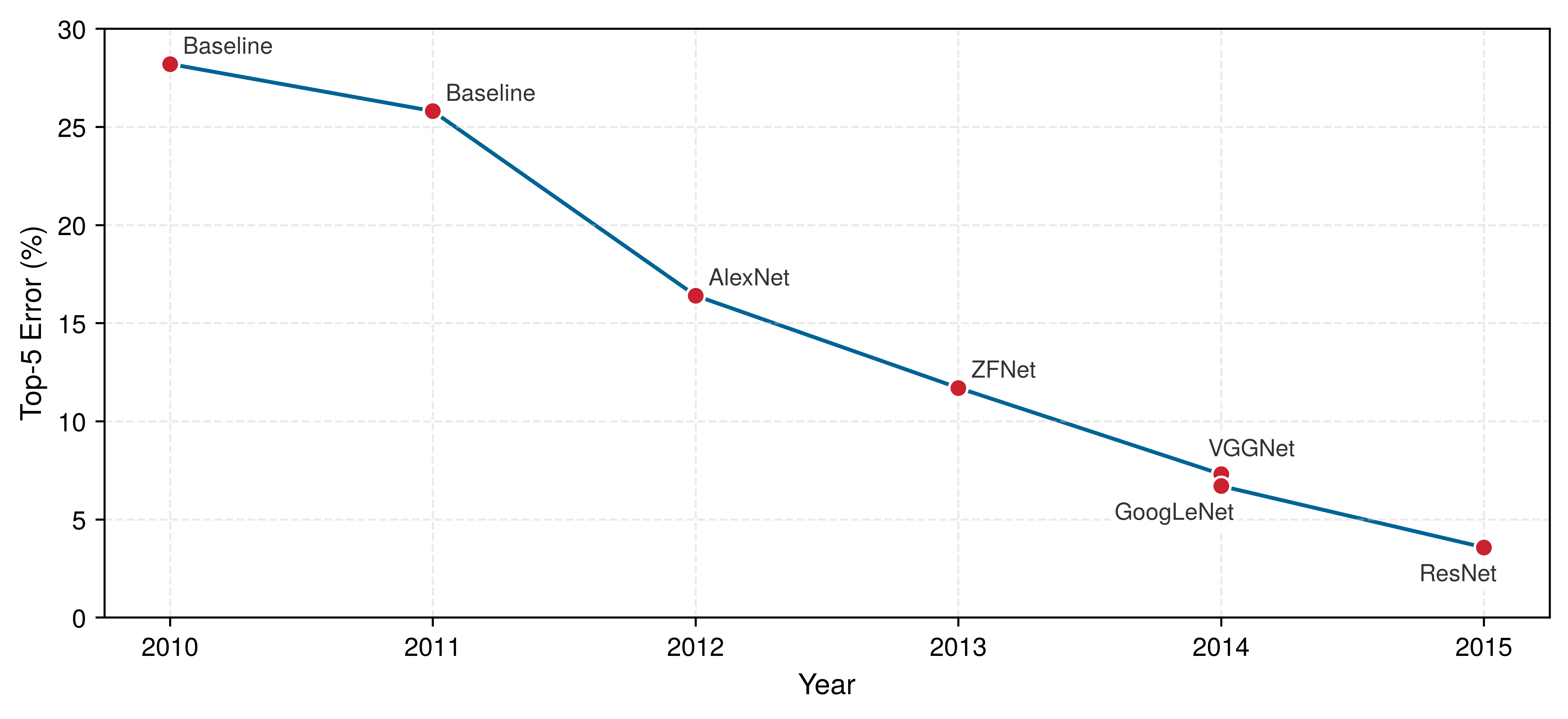
Accuracy metrics and their blind spots

The most common model metrics (accuracy, precision, recall, F1) each reveal different aspects of model behavior while hiding others, and understanding their blind spots is essential for compression validation. Top-\(k\) accuracy measures whether the correct label appears in the model’s top-\(k\) predictions. Top-1 accuracy is strict; top-5 is lenient. The gap between them reveals model uncertainty: a model with 75 percent top-1 but 95 percent top-5 accuracy “knows” the answer is among a few candidates but struggles to commit. For deployment, the acceptable gap depends on whether downstream systems can use ranked predictions or require single answers.

Precision and recall matter when classes are imbalanced or errors have asymmetric costs (Sokolova and Lapalme 2009). A fraud detection model with 99 percent accuracy might have 10 percent recall on actual fraud (catching only one in 10 fraudulent transactions), a catastrophic failure despite high accuracy. Precision (of predicted positives, how many are correct?) and recall (of actual positives, how many were found?) expose these failures that accuracy hides.

Sokolova, Marina, and Guy Lapalme. 2009. “A Systematic Analysis of Performance Measures for Classification Tasks.” Information Processing &Amp; Management 45 (4): 427–37. https://doi.org/10.1016/j.ipm.2009.03.002.

Buolamwini, Joy, and Timnit Gebru. 2018. “Gender Shades: Intersectional Accuracy Disparities in Commercial Gender Classification.” Conference on Fairness, Accountability and Transparency, 77–91.

Most insidiously, aggregate metrics hide subgroup failures. A model achieving 95 percent overall accuracy might achieve 60 percent on a critical demographic subgroup. The Gender Shades project (Buolamwini and Gebru 2018) revealed commercial gender-classification systems for facial analysis performing substantially worse on darker-skinned women than on lighter-skinned men, a disparity invisible to aggregate benchmarks. Disaggregated evaluation across deployment-relevant subgroups is essential; Responsible Engineering examines fairness evaluation systematically.

Calibration: When confidence scores matter

For many deployment scenarios, how confident the model is matters as much as what it predicts. A well-calibrated³⁷ model’s confidence scores correspond to actual correctness probability: when it says “90 percent confident,” it should be correct 90 percent of the time.

³⁷ Calibration: From Arabic qalib (a mold for casting metal) via Latin calibrare, originally describing the adjustment of measuring instruments against known standards. In ML, calibration ensures predicted probabilities match empirical frequencies; Guo et al. (2017) formalize this concern for modern neural networks and show that temperature scaling is a simple effective post-hoc correction. The etymology is apt: just as an uncalibrated instrument produces precise but inaccurate measurements, an uncalibrated model produces confident but unreliable predictions, causing downstream systems that threshold on confidence scores to make systematically wrong decisions.

Guo, Chuan, Geoff Pleiss, Yu Sun, and Kilian Q. Weinberger. 2017. “On Calibration of Modern Neural Networks.” International Conference on Machine Learning (ICML) 70: 1321–30.

Compression can shift calibration even when preserving accuracy, a critical concern when validating quantization techniques from Quantization and Precision. A quantized model might maintain headline accuracy while becoming overconfident on examples it gets wrong. This matters because post-hoc calibration techniques such as temperature scaling can only correct the problem if calibration is measured explicitly (Guo et al. 2017).

Calibration failures create downstream problems. An overconfident model automates errors that it should defer (predicted 95 percent confidence but wrong 30 percent of the time). An underconfident model sends too many correct predictions to review instead of automating decisions it can handle (predicted 70 percent confidence but correct 95 percent of the time). Expected calibration error (ECE) measures the gap between confidence and accuracy across confidence bins; reliability diagrams visualize this correspondence.

Compression validation: The efficiency-quality frontier

Model compression (Model Compression) trades model capacity for efficiency. Validation must determine whether compression achieved an acceptable trade-off or damaged capabilities that matter.

Pareto frontier³⁸ evaluation determines whether a compressed model represents a good trade-off. Plotting accuracy against the target efficiency metric (latency, model size, energy) reveals the trade-off frontier. Models on the Pareto frontier cannot improve one metric without degrading the other; models below the frontier are dominated by better alternatives.

³⁸ Pareto frontier: Named after economist Pareto (1896), the frontier contains all solutions where improving one objective requires degrading another. In compression benchmarking, the frontier’s shape carries diagnostic information: a steep region means efficiency gains come cheaply (prune here), while a flat region means further compression costs disproportionate accuracy (stop here). Points below the frontier are strictly dominated and represent wasted capacity.

Pareto, Vilfredo. 1896. Cours d’économie Politique. F. Rouge.

A dominated model loses on both axes of the Pareto frontier.

Han, Song, Jeff Pool, John Tran, and William J. Dally. 2015. “Learning Both Weights and Connections for Efficient Neural Networks.” Advances in Neural Information Processing Systems 28 (NeurIPS 2015), 1135–43.

Gale, Trevor, Erich Elsen, and Sara Hooker. 2019. “The State of Sparsity in Deep Neural Networks.” arXiv Preprint arXiv:1902.09574.

Hinton, Geoffrey, Oriol Vinyals, and Jeff Dean. 2015. “Distilling the Knowledge in a Neural Network.” arXiv Preprint.

Different compression techniques make different efficiency-quality trade-offs. Quantization reduces precision while often preserving aggregate accuracy (Jacob et al. 2018). Pruning induces sparsity while retaining varying levels of test performance (Han et al. 2015; Gale et al. 2019). Distillation transfers knowledge from a larger teacher or ensemble into a smaller model (Hinton et al. 2015). Because these aggregate results do not establish preserved calibration or tail behavior, validation must measure those properties directly (Guo et al. 2017).

Calibration is a failure mode that aggregate accuracy can hide, and expected calibration error (ECE) is one common diagnostic. ECE compares predicted confidence with empirical accuracy, but it has no universal “good,” “moderate,” or “poor” thresholds. The estimate depends on the binning scheme, bin count, sample size, and prediction distribution. A benchmark must therefore freeze the estimator and compare it with a task-specific tolerance and uncompressed baseline. Compression can leave top-1 accuracy intact while materially changing ECE, which is why a compression protocol measures it directly.

Pareto optimality identifies nondominated choices; it does not establish that any choice clears the deployment’s absolute quality floor. Acceptable degradation depends on deployment context. A 2 percent accuracy drop might be acceptable for a recommendation system (users tolerate imperfect suggestions) but unacceptable for medical diagnosis (each error has significant consequences). Define accuracy thresholds before compression, then validate against them. The acceptance gate must cover aggregate accuracy, calibration, and deployment-critical slices. The MobileNetV2 lighthouse makes the complete INT8 validation protocol concrete.

Lighthouse 1.3: MobileNetV2 INT8 compression

Returning to lighthouse 1.1, consider an illustrative validation protocol for INT8 quantization, grounded in MobileNetV2’s architecture (Sandler et al. 2018) and post-training quantization practice (Jacob et al. 2018). The values in table 18 are assumed:

Precompression baseline: MobileNetV2 achieves 71.8 percent top-1 accuracy on ImageNet at 3.5M parameters (14 MB FP32).

Notice in table 18 that aggregate accuracy barely changes after INT8 quantization to 3.5 MB, but calibration error and edge-case accuracy tell a different story. The INT8 model’s ECE rises from 0.031 to 0.089; whether that increase is acceptable depends on a task-specific tolerance under the fixed ECE protocol.

Table 18: MobileNetV2 INT8 Postcompression Metrics: Illustrative FP32 and INT8 values for top-1 and top-5 accuracy, calibration error, and edge-case accuracy, showing how aggregate accuracy can mask calibration and tail-case degradation.

Metric	FP32	INT8	Acceptable?
Top-1 accuracy	71.8%	70.9%	✓ (0.9 pp drop; below 1 percentage-point threshold)
Top-5 accuracy	91%	90.4%	✓
Calibration ECE	0.031	0.089	No (degraded)
Edge-case accuracy	68.2%	61.4%	No (drop of 6.8 pp)

Edge-case definition: Images with \(>\) 50 percent occlusion, \(<\) 100 lux lighting, or \(>\) 30° rotation from training distribution (approximately 5 percent of real-world inputs).

What this reveals: Under these assumptions, average-case accuracy looks acceptable (0.9 percentage-point drop), but calibration degrades and edge-case accuracy drops 6.8 percentage points. If the deployment uses confidence thresholds (for example, “only act if confidence > 85 percent”) or encounters many edge cases (unusual lighting, partial occlusions), INT8 MobileNetV2 could fail despite passing aggregate benchmarks.

Fix: Apply temperature scaling post-hoc to improve calibration (Guo et al. 2017). Temperature scaling learns a single scalar \(T_{\text{cal}}\) to divide logits before softmax: \(\text{softmax}(z_i/T_{\text{cal}})\). In parallel, add edge-case examples to the test set to monitor that specific failure mode continuously.

Jacob, Benoit, Skirmantas Kligys, Bo Chen, Menglong Zhu, Matthew Tang, Andrew Howard, Hartwig Adam, and Dmitry Kalenichenko. 2018. “Quantization and Training of Neural Networks for Efficient Integer-Arithmetic-Only Inference.” 2018 IEEE/CVF Conference on Computer Vision and Pattern Recognition, 2704–13. https://doi.org/10.1109/cvpr.2018.00286.

Sandler, Mark, Andrew Howard, Menglong Zhu, Andrey Zhmoginov, and Liang-Chieh Chen. 2018. “MobileNetV2: Inverted Residuals and Linear Bottlenecks.” 2018 IEEE/CVF Conference on Computer Vision and Pattern Recognition, 4510–20. https://doi.org/10.1109/cvpr.2018.00474.

Frankle, Jonathan, and Michael Carbin. 2019. “The Lottery Ticket Hypothesis: Finding Sparse, Trainable Neural Networks.” International Conference on Learning Representations (ICLR).

The Lottery Ticket Hypothesis (Lottery ticket hypothesis) provides concrete benchmarking data illustrating what Pareto-efficient compression looks like. Through iterative pruning, Frankle and Carbin (2019) found sparse subnetworks (“winning tickets”) in fully connected and convolutional networks that could match the original network’s test accuracy when trained in isolation.

The Lottery Ticket results reveal the shape of compression trade-offs: aggressive pruning can preserve accuracy for some architectures and tasks, but the acceptable sparsity point is empirical rather than universal. Compression validation should establish similar trade-off curves for each specific model and task, identifying where the model sits on the Pareto frontier and whether further compression yields meaningful efficiency gains or merely degrades quality.

Large language model benchmarks

The compression evaluation framework applies cleanly when the task has a stable label: classification accuracy, detection mAP, segmentation IoU. Large language models break that pattern. A team can choose a model because it scores well on a public benchmark, then discover in deployment that the model recognizes multiple-choice facts but cannot generate a grounded answer, responds too slowly for an interactive product, or produces confident unsafe text that the benchmark never stressed. LLM benchmarking therefore starts by naming the deployment failure that a score is meant to rule out.

The useful LLM metric taxonomy in table 19 is therefore a decision aid, not a leaderboard. Its rows use Massive Multitask Language Understanding (MMLU),³⁹ HELM (Holistic Evaluation of Language Models),⁴⁰ and perplexity⁴¹ as examples of scores that answer different deployment questions:

³⁹ MMLU (massive multitask language understanding): Introduced by Hendrycks et al. (2020) with 15,908 multiple-choice questions across fifty-seven subjects. MMLU’s benchmarking limitation is its format: multiple-choice recognition is not the same task as open-ended generation, so an MMLU score should not be read as direct evidence that a model can produce grounded free-form answers in production.

Hendrycks, Dan, Collin Burns, Steven Basart, Andy Zou, Mantas Mazeika, Dawn Song, and Jacob Steinhardt. 2020. “Measuring Massive Multitask Language Understanding.” arXiv Preprint.

⁴⁰ HELM (holistic evaluation of language models): Stanford’s 2022 evaluation framework tested a broad set of models across seven dimensions (accuracy, calibration, robustness, fairness, bias, toxicity, efficiency) (Liang et al. 2022). HELM’s contribution is methodological: by evaluating models that score similarly on accuracy but diverge on calibration or toxicity, it demonstrates that single-metric leaderboards systematically hide failure modes that matter for production deployment.

Liang, Percy, Rishi Bommasani, Tony Lee, Dimitris Tsipras, Dilara Soylu, Michihiro Yasunaga, Yian Zhang, et al. 2022. “Holistic Evaluation of Language Models.” arXiv Preprint arXiv:2211.09110.

⁴¹ Perplexity: From Latin perplexus (entangled); in information theory, \(2^{H(p)}\) where \(H\) is entropy. A perplexity of 10 means the model is “10-way confused” on average. The systems consequence is interpretive rather than direct memory accounting: perplexity measures held-out next-token prediction on a corpus, while serving memory pressure is governed by context length, batch size, model shape, and decoding state; KV-cache management is a separate serving problem (Kwon et al. 2023).

Kwon, Woosuk, Zhuohan Li, Siyuan Zhuang, Ying Sheng, Lianmin Zheng, Cody Hao Yu, Joseph Gonzalez, Hao Zhang, and Ion Stoica. 2023. “Efficient Memory Management for Large Language Model Serving with PagedAttention.” Proceedings of the 29th Symposium on Operating Systems Principles, 611–26. https://doi.org/10.1145/3600006.3613165.

Table 19: Failure-Oriented LLM Benchmark Taxonomy: LLM metrics are useful when each score is tied to the deployment failure it is meant to rule out. Recognition, holistic behavior, corpus prediction, and responsiveness expose different risks, so no single score establishes production readiness.

Deployment failure to rule out	Metric or benchmark family	What the score reveals	What the score cannot prove
The model recognizes facts poorly	MMLU (Massive Multitask Language Understanding)	Broad factual and disciplinary knowledge across fifty-seven subjects, with scores interpretable against chance-level multiple-choice performance	Whether the model can generate grounded open-ended answers rather than choose among multiple-choice options
The model is capable but unsafe	HELM (Holistic Evaluation of Language Models)	Accuracy alongside calibration, robustness, fairness, bias, toxicity, and efficiency	Whether one aggregate score captures the deployment risk; a model can be strong on accuracy and weak on calibration, safety, cost, or prompt stability
The model predicts its corpus well	Perplexity	Held-out next-token prediction on the same corpus; a perplexity of 10 means the model is “10-way confused” on average	Whether generated answers are helpful, safe, or grounded outside that corpus
The model feels slow in use	First-token latency, inter-token latency, and token throughput	Prompt-processing delay before generation starts and decode speed after generation begins	Whether a single throughput number hides poor interactive responsiveness, especially when batching improves throughput but worsens first-token latency

The responsiveness row deserves a concrete timing anchor because LLM benchmarks often report a single throughput number even though users experience generation in phases. A model can look efficient in tokens per second while still feeling slow if the first token arrives late, or it can improve first-token latency while producing the rest of the answer too slowly for an interactive workflow. The token throughput calculation turns those token-rate metrics into user-visible wall-clock time.

Token throughput turns that trade-off into wall-clock time. For a response of about 750 tokens, 25 tokens/s means 30 seconds of generation, while 100 tokens/s means 7.5 seconds. Time-to-first-token and inter-token latency must therefore be reported together: one captures responsiveness at the start of the exchange, and the other captures the rate at which the answer arrives.

The final failure is that a score may measure memory rather than capability. Benchmark contamination is a unique LLM risk because models trained on web-scale corpora may encounter benchmark questions during pretraining, inflating scores through memorization rather than skill (Xu et al. 2024). Leakage detection reframes this risk as something benchmark designers can test for rather than merely suspect. Temporal holdouts use content published after the training cutoff, dynamic benchmarks generate fresh instances continuously, and contamination tests ask whether the model recalls exact benchmark phrasing. These techniques keep the benchmark aligned with the deployment question instead of rewarding exposure to the test set.

Xu, Ruijie, Zengzhi Wang, Run-Ze Fan, and Pengfei Liu. 2024. “Benchmarking Benchmark Leakage in Large Language Models.” arXiv Preprint arXiv:2404.18824.

Data benchmarking

Model benchmarks validate whether compression preserved model quality. Model quality, however, depends entirely on the data used to train and evaluate it, and this dependency creates the most insidious failure mode in ML deployment. A perfectly preserved model trained on biased or unrepresentative data will still fail in production. Data benchmarks validate whether the efficiency strategies from Data Selection (active learning, curriculum design, data augmentation, and synthetic data generation) produced training sets that enable reliable deployment. This is often the last validation to fail and the hardest to diagnose: a model achieving excellent accuracy on held-out test data may collapse on production inputs that the training data never adequately represented.

Contemporary AI development has made clear that data quality can set a performance boundary that architecture changes alone cannot overcome. This recognition elevated data benchmarking from afterthought to critical discipline.

A data benchmark therefore starts with a protocol before it starts with a score. Define the deployment slice the model must serve, reserve a leakage-resistant holdout, verify duplicate and near-duplicate separation across partitions, set minimum coverage for rare classes and subgroups, audit label quality, and establish drift thresholds that determine when the benchmark no longer represents production. Only after those gates are explicit do aggregate metrics become interpretable.

Coverage metrics

The first question data benchmarking must answer is whether the training data represents the inputs the model will encounter. A model cannot learn patterns it has never seen, and the ways training data can fail to represent deployment reality are often subtle.

Consider class balance: a fraud detection dataset with 99 percent legitimate transactions and 1 percent fraud might produce a model that achieves 99 percent accuracy by simply labeling everything legitimate. The model is useless, but the accuracy metric looks excellent. Severe imbalance often requires mitigation through oversampling, class weighting, or threshold adjustment. More insidious is subgroup imbalance within classes: a dataset might have balanced positive and negative examples overall, but negative examples might be drawn predominantly from one demographic group, creating disparities invisible to aggregate class balance metrics.

Feature coverage presents an even harder challenge because it requires domain knowledge about what variations matter. A computer vision model trained exclusively on daytime images will fail on nighttime inputs; a natural language model trained on formal text will fail on colloquial language. Unlike class balance, which can be computed from labels alone, feature coverage requires understanding the deployment context. The lighting conditions the camera will encounter, the dialects users will speak, and the edge cases that exist in production but never appear in test sets all fall outside what labels alone can predict. These questions have no algorithmic answer; they demand collaboration between ML engineers and domain experts who understand the deployment environment.

For applications affecting people, demographic representation becomes a coverage dimension with ethical implications. Training data must represent the deployment population across relevant dimensions: age, gender, ethnicity, geography, language. A facial recognition system trained predominantly on one demographic group may underperform on others, even if aggregate accuracy metrics look acceptable. The challenge is that demographic metadata is often unavailable or unreliable, making representation gaps difficult to detect and measure.

Quality metrics

Even when training data covers the right inputs, the labels themselves may be unreliable. Studies consistently find 3–6 percent label error rates in major datasets, including ImageNet (Northcutt et al. 2021). These errors are not merely noise—they become learned ground truth. A model trained on data where wolves are occasionally labeled as dogs will learn the false rule that some wolves are dogs. The benchmark will report this as correct behavior because the model matches the (incorrect) labels.

Northcutt, Curtis G., Anish Athalye, and Jonas Mueller. 2021. “Pervasive Label Errors in Test Sets Destabilize Machine Learning Benchmarks.” arXiv Preprint arXiv:2103.14749 34: 19075–90. https://doi.org/10.48550/arxiv.2103.14749.

For small datasets, manual audit of a random sample can estimate label accuracy. For large datasets, confident learning techniques identify likely mislabeled examples by finding cases where model predictions systematically disagree with labels. The intuition is that when a model confidently predicts a different label than the ground truth, either the model has learned something incorrect or the label is wrong. Detection, however, is only the first step; correction requires human review, and scaling human review to millions of examples presents its own challenges.

Inter-annotator agreement provides a different lens on label quality by measuring consistency across human labelers. Cohen’s kappa or Fleiss’ kappa quantify agreement beyond what chance would produce (Cohen 1960; Fleiss 1971). When agreement falls below conventional thresholds for tasks with clear ground truth, something is wrong: either the labeling guidelines are ambiguous, the task is inherently subjective, or labeler quality varies significantly. Landis and Koch’s qualitative kappa bands are widely cited as a rough interpretive guide, though they should not replace domain judgment (Landis and Koch 1977).

Cohen, Jacob. 1960. “A Coefficient of Agreement for Nominal Scales.” Educational and Psychological Measurement 20 (1): 37–46. https://doi.org/10.1177/001316446002000104.

Fleiss, Joseph L. 1971. “Measuring Nominal Scale Agreement Among Many Raters.” Psychological Bulletin 76 (5): 378–82. https://doi.org/10.1037/h0031619.

Landis, J. Richard, and Gary G. Koch. 1977. “The Measurement of Observer Agreement for Categorical Data.” Biometrics 33 (1): 159–74. https://doi.org/10.2307/2529310.

The distinction between random and systematic errors matters enormously for their downstream effects. Unstructured label noise can be less damaging than a consistent bias because its errors do not all reinforce the same false rule, although modern models can still memorize it. Systematic errors (consistently mislabeling a particular subclass), in contrast, teach a coherent but wrong association. A dataset where all wolves photographed in snow are labeled “dogs” can produce a model that calls snowy wolves dogs, and adding more data with the same labeling rule only reinforces the error.

Distribution alignment

The final category of data benchmarking asks whether models will generalize from training conditions to deployment reality. This train-to-production alignment question is where the gap between benchmark performance and production performance most frequently emerges.

The standard assumption underlying held-out evaluation, that test data comes from the same distribution as training data, is routinely violated in practice. Test sets constructed years after training data may reflect distribution drift as the world changes. Test sets from different geographic regions may reflect population shift. A model with strong held-out accuracy can drop sharply when deployed to a region or time period the test set did not represent. Once the i.i.d. (independent and identically distributed) assumption fails, held-out performance no longer identifies deployment performance and is often optimistic when the deployment distribution is harder.

The true test is train-to-production alignment, and this is far harder to measure because production data differs from training data in ways that held-out test sets often fail to capture. Production images come from different cameras with different characteristics. Production users come from different populations with different behaviors. Production inputs include edge cases that curated test sets systematically exclude. The WILDS⁴² benchmark (Koh et al. 2021) was designed specifically to evaluate models under realistic distribution shifts: hospital systems with different patient populations, wildlife cameras at different locations, satellite imagery from different time periods. On Camelyon17-WILDS, the reported ERM baseline achieved 93.2 percent in-distribution average accuracy and 70.3 percent out-of-distribution average accuracy.

⁴² WILDS: Stanford’s 2021 benchmark of ten datasets with real-world distribution shifts: hospital changes (Camelyon17), wildlife camera location shifts (iWildCam), and satellite imagery temporal drift (PovertyMap). For the reported Camelyon17-WILDS ERM baseline, average accuracy fell from 93.2 percent in-distribution to 70.3 percent out-of-distribution, demonstrating that standard held-out evaluation can overestimate performance when the i.i.d. assumption fails.

Koh, Pang Wei, Shiori Sagawa, Henrik Marklund, Sang Michael Xie, Marvin Zhang, Akshay Balsubramani, Weihua Hu, et al. 2021. “WILDS: A Benchmark of in-the-Wild Distribution Shifts.” In Proceedings of the 38th International Conference on Machine Learning, ICML 2021, 18-24 July 2021, Virtual Event, edited by Marina Meila and Tong Zhang, vol. 139, 139. Proceedings of Machine Learning Research. PMLR.

Berger, Vance W., and YanYan Zhou. 2014. “Kolmogorov–Smirnov Test: Overview.” In Wiley StatsRef: Statistics Reference Online. Wiley. https://doi.org/10.1002/9781118445112.stat06558.

Gretton, Arthur, Karsten M. Borgwardt, Malte J. Rasch, Bernhard Schölkopf, and Alexander Smola. 2012. “A Kernel Two-Sample Test.” Journal of Machine Learning Research 13 (25): 723–73.

Given these challenges, shift detection methods become essential for production monitoring. Statistical tests like the Kolmogorov-Smirnov test (Berger and Zhou 2014) or kernel-based two-sample tests such as maximum mean discrepancy (Gretton et al. 2012) can detect covariate shift—when the distribution of inputs changes even if the relationship between inputs and outputs remains stable. Monitoring model confidence distributions can detect when the model encounters inputs unlike anything in training. The goal is early detection: identifying distribution shift before it causes catastrophic performance degradation, enabling intervention through model updates, data collection, or deployment constraints.

Distribution alignment challenges highlight a persistent tension in ML development between two paradigms: fixing the data and iterating on models, or fixing the model and iterating on data. Figure 12 places these two paradigms side by side, revealing exactly where the feedback loop differs. In the model-centric diagram, the iteration cycle targets the architecture while the data remains static; in the data-centric diagram, the architecture stays fixed while the cycle targets data quality. The two approaches are complementary rather than a universal ranking of where improvement will come from.

\begin{tikzpicture}[font=\sffamily]
\tikzset{Line/.style={line width=1.25pt,black!50,-{Latex[length=3mm,width=2mm]}}
}
%CPU
\tikzset{%
 pics/cpu/.style = {
        code = {
        \pgfkeys{/channel/.cd, #1}
\begin{scope}[local bounding box=CPU\picname,scale=\scalefac, every node/.append style={transform shape}]
\node[fill=\filllcolor,minimum width=66, minimum height=66,
            rounded corners=2,outer sep=2pt] (C1) {};
\node[fill=white,minimum width=54, minimum height=54] (C2) {};
\node[fill=\filllcolor!40,minimum width=44, minimum height=44] (C3) {\large CPU};

\foreach \x/\y in {0.11/1,0.26/2,0.41/3,0.56/4,0.71/5,0.85/6}{
\node[fill=\filllcolor,minimum width=3, minimum height=15,
           inner sep=0pt,anchor=south](GO\y)at($(C1.north west)!\x!(C1.north east)$){};
}
\foreach \x/\y in {0.11/1,0.26/2,0.41/3,0.56/4,0.71/5,0.85/6}{
\node[fill=\filllcolor,minimum width=3, minimum height=15,
           inner sep=0pt,anchor=north](DO\y)at($(C1.south west)!\x!(C1.south east)$){};
}
\foreach \x/\y in {0.11/1,0.26/2,0.41/3,0.56/4,0.71/5,0.85/6}{
\node[fill=\filllcolor,minimum width=15, minimum height=3,
           inner sep=0pt,anchor=east](LE\y)at($(C1.north west)!\x!(C1.south west)$){};
}
\foreach \x/\y in {0.11/1,0.26/2,0.41/3,0.56/4,0.71/5,0.85/6}{
\node[fill=\filllcolor,minimum width=15, minimum height=3,
           inner sep=0pt,anchor=west](DE\y)at($(C1.north east)!\x!(C1.south east)$){};
}
 \end{scope}
     }
  }
}
%CPU
\tikzset{mycylinder/.style={cylinder, shape border rotate=90, aspect=1.3, draw, fill=white,
minimum width=25mm,minimum height=11mm,line width=\Linewidth,node distance=-0.15},
pics/data/.style = {
        code = {
        \pgfkeys{/channel/.cd, #1}
\begin{scope}[local bounding box=DATA\picname,scale=\scalefac, every node/.append style={transform shape}]
\node[mycylinder,fill=\filllcolor!50] (A) {};
\node[mycylinder, above=of A,fill=\filllcolor!30] (B) {};
\node[mycylinder, above=of B,fill=\filllcolor!10] (C) {};
\fill[\filllcolor!50!black]($(C.west)!0.12!(C.east)$)circle(3pt);
\fill[\filllcolor!50!black]($(B.west)!0.12!(B.east)$)circle(3pt);
\fill[\filllcolor!50!black]($(A.west)!0.12!(A.east)$)circle(3pt);
 \end{scope}
     }
  }
}
%lokot
\tikzset{
pics/lokot/.style = {
        code = {
        \pgfkeys{/channel/.cd, #1}
\begin{scope}[shift={($(0,0)+(0,0)$)},scale=\scalefac,every node/.append style={transform shape}]
\fill[fill=\filllcolor](0,0)--(2.7,0)--++(270:1.6)to[out=270,in=0](1.85,-2.45)
--++(180:1.1)to[out=180,in=270](0,-1.3)--cycle;
\fill[fill=white](1.32,-0.9)+(230:0.3)
arc[start angle=230, end angle=-50, radius=0.3]--++(280:0.75)--++(180:0.62)--cycle;
\path[](0.27,0)circle(1pt)coordinate(K1);
\path[](0.57,0)circle(1pt)coordinate(K2);
\path[](2.10,0)circle(1pt)coordinate(K3);
\path[](2.4,0)circle(1pt)coordinate(K4);
%
\path[](K1)--++(90:0.6)coordinate(KK1);
\path[](K2)--++(90:0.5)coordinate(KK2);
\path[](K4)--++(90:0.6)coordinate(KK4);
\path[](K3)--++(90:0.5)coordinate(KK3);
\fill[fill=\filllcolor](K1)--(KK1)to[out=90,in=90,distance=37](KK4)--(K4)
--(K3)--(KK3)to[out=90,in=90,distance=29](KK2)--(K2)--cycle;
\end{scope}
    }
  }
}
\pgfkeys{
  /channel/.cd,
   Depth/.store in=\Depth,
  Height/.store in=\Height,
  Width/.store in=\Width,
  filllcirclecolor/.store in=\filllcirclecolor,
  filllcolor/.store in=\filllcolor,
  drawcolor/.store in=\drawcolor,
  drawcircle/.store in=\drawcircle,
  scalefac/.store in=\scalefac,
  Linewidth/.store in=\Linewidth,
  picname/.store in=\picname,
  filllcolor=BrownLine,
  filllcirclecolor=violet!20,
  drawcolor=black,
  drawcircle=violet,
  scalefac=1,
  Linewidth=0.5pt,
  Depth=1.3,
  Height=0.8,
  Width=1.1,
  picname=C
}

%Data
\pic[shift={(0,0)}] at  (0,0){data={scalefac=0.75,picname=1,filllcolor=RedLine, Linewidth=1.0pt}};
%padlock
\pic[shift={(0,0)}] at  (0.5,2){lokot={scalefac=0.22,picname=1,drawcolor=OrangeLine!70!,
filllcolor=black!,Linewidth=0.7pt, filllcirclecolor=black}};
%CPU
\pic[shift={(0,-0.2)}] at  (4.5,1){cpu={scalefac=0.6,picname=1,filllcolor=BlueLine, Linewidth=0.7pt}};
\node[below=0.15 of DO3](MO){Model};
\path[red](MO)-|coordinate(D)(A);
\node[]at(D){Data};
\draw[Line,shorten <=4pt,shorten >=11pt](B.east)--++(0:25mm);
\draw[Line,shorten <=8pt,shorten >=8pt,]($(DE3)!0.5!(DE4)$)--++(0:1)--++(90:1.8)-|
node[above,text=black](TXT){Systematically enhance the model}($(GO3)!0.5!(GO4)$);
%
\scoped[on background layer]
\node[draw=BackLine,inner xsep=5mm,inner ysep=5mm,
yshift=2mm,
fill=BackColor,fit=(D)(DATA1)(CPU1)(TXT),line width=0.75pt](BB){};
\node[below=4pt of  BB.north,inner sep=0pt,xshift=3,
anchor=north,fill=BackColor]{\textbf{Model-centric AI}};
%%%%%%%%%%%%%%%%%
%right
%%%%%%%%%%%%%%%%%%%%
\begin{scope}[node distance=-0.15,shift={(13.5,0)},local bounding box = 2DATA]
\pic[shift={(0,0)}] at  (0,0){data={scalefac=0.75,picname=2,filllcolor=RedLine, Linewidth=1.0pt}};
\pic[shift={(0,-0.2)}] at  (4.5,1){cpu={scalefac=0.6,picname=2,filllcolor=BlueLine, Linewidth=0.7pt}};
\pic[shift={(0,0)}] at  (4.75,1.69){lokot={scalefac=0.22,picname=2,drawcolor=OrangeLine!70!,
filllcolor=black!,Linewidth=0.7pt, filllcirclecolor=black}};
%
\draw[Line,shorten <=4pt,shorten >=11pt](B)--($(LE3)!0.5!(LE4)$);

\node[below=0.15of CPU2](2MO){Model};
\path[red](2MO)-|coordinate(2D)(DATA2);
\node[]at(2D){Data};

\draw[Line](CPU2.east)--++(0:1)coordinate(DE)--++(90:1.8)-|
           node[above,text=black,pos=0.25](2TXT){Systematically enhance the data}(DATA2);
%
\scoped[on background layer]
\node[draw=GreenLine,inner xsep=5mm,inner ysep=5mm,
           yshift=2mm, fill=GreenL!50,fit=(2D)(DATA2)(CPU2)(2TXT)(DE),line width=0.75pt](2BB){};
\node[below=4pt of  2BB.north,inner sep=0pt,xshift=3,
           anchor=north]{\textbf{Data-centric AI}};
\end{scope}
%%%%
\node[double arrow, fill=red!80!black!90,
           minimum width = 10pt, double arrow head extend=4pt,
           minimum height=35mm](DA) at($(BB.east)!0.5!(2BB.west)$){};
\node[below=0.2of DA]{Complementary};
 \end{tikzpicture}

Figure 12: Development Paradigms: Model-centric AI iterates on architecture while holding the dataset fixed, whereas data-centric AI iterates on annotations, diversity, and bias while holding the architecture fixed. The double arrow marks the approaches as complementary.

Data-centric AI reflects an important shift in understanding that challenges the “more data is always better” assumption: dataset composition matters alongside scale. Initiatives like DataPerf (Mazumder et al. 2023) and DataComp⁴³ have emerged to evaluate how dataset construction affects model performance systematically. In DataComp’s compute-controlled setting, a baseline that retained the top 30 percent of the candidate pool by CLIP-based filtering outperformed the unfiltered-pool baseline on aggregate downstream evaluation (Gadre et al. 2023). The result establishes the value of curation for that protocol, not a universal optimal fraction.

Mazumder, Mark, Colby Banbury, Xiaozhe Yao, Bojan Karlaš, et al. 2023. “DataPerf: Benchmarks for Data-Centric AI Development.” Advances in Neural Information Processing Systems 36.

⁴³ DataComp: Introduced in 2023, DataComp fixes the model family, training code, and compute budget while participants vary dataset construction. Its filtering track isolates the effect of selecting examples from a common candidate pool, making curation strategies comparable without attributing every gain to additional training compute.

Gadre, Samir Yitzhak, Gabriel Ilharco, Alex Fang, Jonathan Hayase, Georgios Smyrnis, Thao Nguyen, Ryan Marten, et al. 2023. “DataComp: In Search of the Next Generation of Multimodal Datasets.” Advances in Neural Information Processing Systems (NeurIPS) 36: 27092–112. https://doi.org/10.52202/075280-1179.

A persistent challenge in data benchmarking emerges from dataset saturation. When models achieve near-perfect accuracy on benchmarks like ImageNet, practitioners must distinguish whether performance gains represent genuine capability advances or merely optimization to existing test sets. As the timeline in figure 13 illustrates, widely tracked AI benchmarks have repeatedly crossed reported human baselines, making each corresponding benchmark less useful as a differentiator (Maslej et al. 2024).

\begin{tikzpicture}[font=\small\sffamily]
%\node[anchor=south west]at(-0.93,-0.76){%
%\includegraphics[scale=0.7]{1}};

\begin{axis}[clip=false,
   axis line style={draw=none},
  /pgf/number format/.cd,
 1000 sep={},
  width=155mm,%155.9mm,
  height=80mm,%58.0mm,
  axis x line*=bottom,
  legend style={at={(0.16,0.98)}, anchor=north},
  legend cell align=left,
  title style={yshift=-2pt,font=\fontsize{9pt}{9}\selectfont\sffamily},
  ylabel style={align=center,font=\footnotesize\sffamily},
  xmin=1997,
  xmax=2022,
  xtick={2000,2005,2010,2015,2020},
   x tick label style={rotate=0, anchor=north},
  ymin=-100, ymax=24,
  ytick={-100,-80,...,20},
  yticklabels={$-$100,$-$80,$-$60,$-$40,$-$20,0,+20},
  ylabel={Test score of the AI relative\\ to human performance},
  title={Language and image recognition capabilities of AI systems have improved rapidly},
  grid=both,
  major grid style={black!60},
  minor grid style={draw=none},
  minor x tick num=4,
  minor x tick  style={thin,black!60},
  tick label style={/pgf/number format/assume math mode=true},
  ticklabel style={font=\footnotesize\sffamily},
  xticklabel style={yshift=-3pt},
]
%Handwriting recognition
\addplot[OrangeLine,mark=*,
mark size=2pt,line width=1.5pt,
]
coordinates{
(1998,-100)(1998,-80)(2002,-48)(2003,-27)(2006,-25)(2010,-20)(2012,-5)(2013,-1)(2018,2)
}node[pos=0.67,above=3mm]{Handwriting recognition};
%Speech recognition
\addplot[RedLine,mark=*,
mark size=2.0pt,line width=1.5pt,
] coordinates{
(1998,-100)(2011,-66)(2013,-53)(2014,-28)(2015,-26)(2015,-9)(2016,-5)(2016,-1.2)(2017,0.5)(2018,2)
}node[pos=0.17,above=3mm]{Speech recognition};
%Image recognition
\addplot[GreenD,mark=*,
mark size=2.0pt,line width=1.5pt,
] coordinates{
(2009,-100)(2012,-44)(2014,-11.5)(2014,-7)(2015,1)(2016,6)(2018,11.5)(2019,9)(2020,16)
}node[pos=0.13,left=2mm,anchor=north east]{Image recognition};
%Reading comprehension
\addplot[cyan!90!black,mark=*,
mark size=2.0pt,line width=1.5pt,
] coordinates{
(2016,-100)(2016,-34)(2017,-30)(2017,-9)(2018,6)(2019,18)(2020,19)
}node[pos=0.23,left=2mm,anchor=north east,align=right]{Reading\\ comprehension};
%Language understanding
\addplot[red,mark=*,
mark size=2.0pt,line width=1.5pt,
] coordinates{
(2018,-100)(2018,-68)(2019,-64)(2019,-25)(2019,0)(2019,4)(2020,8)(2020,12)
}node[pos=0.23,right=2mm,anchor=north west,align=left]{Language\\ understanding};
%
\draw[font=\fontsize{7pt}{9}\selectfont\sffamily,latex-](axis cs:1996.5,-104)to[bend right=25]++(320:9mm)
node[align=left,below right=2mm and 1mm,anchor=west]{The capability of each AI system is normalized\\
to an initial performance $-$100};
\draw[font=\fontsize{7pt}{9}\selectfont\sffamily,latex-](axis cs:1996.8,2)to[bend left=25]++(30:6mm)
node[align=left, right=1mm,anchor=west]{Human performance, as the benchmark, is set to zero};
%
\draw[red,line width=2pt,{Triangle[width=6pt,length=5pt]}-{Triangle[width=5pt,length=6pt]}](axis cs:2021,-1)--
node[font=\fontsize{7pt}{9}\selectfont\sffamily,right,text=black]{AI systems perform worse}
(axis cs:2021,-19);
\draw[red,line width=2pt,{Triangle[width=6pt,length=5pt]}-{Triangle[width=5pt,length=6pt]}](axis cs:2021,1)--
node[align=left,font=\fontsize{7pt}{9}\selectfont\sffamily,right,text=black]{AI systems perform better than\\
the humans who did these tests}
(axis cs:2021,19);
\coordinate(A)at(axis cs:1994,-100);
\coordinate(B)at(axis cs:2027.5,-100);
\coordinate(C)at(axis cs:2027.5,0);
\coordinate(C1)at(axis cs:2027.5,25);
\coordinate(D)at(axis cs:1994,0);
\coordinate(D1)at(axis cs:1994,25);
\scoped[on background layer]
\fill[fill=magenta!5](A)--(B)--(C)--(D)--cycle;
\scoped[on background layer]
\fill[fill=green!5](D)--(C)--(C1)--(D1)--cycle;
\end{axis}
\end{tikzpicture}

Figure 13: Dataset Saturation: The zero line denotes reported human performance; each curve’s crossing marks a capability for which the static benchmark has less remaining discriminating headroom. The crossings do not distinguish genuine capability gains from optimization to the evaluation set. Sources: (Maslej et al. 2024; Kiela et al. 2021).

Maslej, Nestor, Loredana Fattorini, C. Raymond Perrault, Vanessa Parli, Anka Reuel, Erik Brynjolfsson, John Etchemendy, et al. 2024. “Artificial Intelligence Index Report 2024.” In CoRR, vol. abs/2405.19522, abs/2405.19522. https://doi.org/10.48550/ARXIV.2405.19522.

Dataset saturation and dynamic benchmarks

Figure 13 raises a critical methodological problem: when models surpass human performance on benchmarks, the result may reflect either genuine capability advances or optimization to static evaluation sets, and the two are difficult to distinguish from leaderboard scores alone. MNIST, introduced through the classic handwritten-digit recognition work of LeCun and colleagues (LeCun et al. 1998), illustrates the concern: static test images can contain dataset-specific artifacts that models learn to exploit. The question “Are we done with ImageNet?” (Beyer et al. 2020) generalizes this concern.

LeCun, Yann, Léon Bottou, Yoshua Bengio, and Patrick Haffner. 1998. “Gradient-Based Learning Applied to Document Recognition.” Proceedings of the IEEE 86 (11): 2278–324. https://doi.org/10.1109/5.726791.

Beyer, Lucas, Olivier J. Hénaff, Alexander Kolesnikov, Xiaohua Zhai, and Aäron van den Oord. 2020. “Are We Done with ImageNet?” arXiv Preprint arXiv:2006.07159.

⁴⁴ Dynabench: Facebook AI Research’s 2021 platform for dynamic benchmark generation, where humans craft adversarial inputs that fool current best models. Dynabench addresses the saturation problem, where very high accuracy on static benchmarks may reflect test-set familiarity rather than robust capability, but introduces its own trade-off: dynamic benchmarks are harder to compare across time because the evaluation set changes. Static and dynamic benchmarks serve complementary diagnostic roles.

Kiela, Douwe, Max Bartolo, Yixin Nie, Divyansh Kaushik, Atticus Geiger, Zhengxuan Wu, Bertie Vidgen, et al. 2021. “Dynabench: Rethinking Benchmarking in NLP.” Proceedings of the 2021 Conference of the North American Chapter of the Association for Computational Linguistics: Human Language Technologies 9: 4110–24. https://doi.org/10.18653/v1/2021.naacl-main.324.

Dynamic benchmarking approaches like Dynabench⁴⁴ (Kiela et al. 2021) address saturation by continuously evolving test data based on model performance, ensuring that benchmarks remain challenging as capabilities improve. However, dynamic benchmarks complement rather than replace the coverage, quality, and distribution metrics described earlier: they prevent saturation but do not diagnose its causes.

Holistic system-model-data evaluation

Passing system, model, and data benchmarks independently is not enough. A system benchmark can validate hardware performance, a model benchmark can verify that compression preserved quality, and a data benchmark can assess training set representativeness, yet the deployed system can still fail because the three dimensions interact. Real-world AI performance emerges from that interaction, and optimizing one dimension can expose weaknesses in another.

Consider a concrete failure cascade: a team achieves excellent MLPerf Inference scores by deploying an INT8-quantized model on optimized hardware. System benchmarks pass. The quantized model, however, was validated only on ImageNet-distributed test data; deployment reveals accuracy degradation on factory-floor images with different lighting characteristics. Model quality benchmarks would have caught the quantization sensitivity. Further investigation shows the training data contained no images with industrial lighting—a data quality gap that no amount of system or model optimization can address.

This interdependence means that benchmark results from one dimension can be invalidated by failures in another:

• System success + Model failure: Hardware delivers promised throughput, but compression degraded accuracy below deployment thresholds
• System success + Data failure: Fast inference on representative inputs, but training data bias causes failures on demographic subgroups
• Model success + System failure: Accurate predictions, but latency variance under load violates SLA requirements
• Model success + Data failure: High accuracy on held-out test set, but distribution shift in production causes silent degradation

This interdependence echoes the D·A·M landscape introduced in Introduction (The D·A·M Intersection Landscape), but the benchmark lenses do not map one-to-one onto its axes. Data benchmarks primarily test the evidence supplied to learning; model benchmarks primarily test learned algorithmic behavior; and system benchmarks expose machine execution together with the data movement and software needed to drive it. Holistic evaluation verifies that assumptions made in one lens still hold where the D·A·M axes interact. The Part III optimization pipeline (data → model → hardware) creates dependencies that benchmarking must validate explicitly.

The D·A·M taxonomy provides a diagnostic framework for systematically identifying which axis limits performance. Diagnostic Summary maps each axis to its binding physical constraint and the optimization pathway that relieves it, giving the first diagnostic step when a benchmark reveals underutilization. Table 20 formalizes this approach by crossing each D·A·M axis with the three fundamental bottleneck types; The D·A·M Taxonomy gives the full diagnostic guide, including profiling utilities and efficiency screening indicators.

Table 20: D·A·M Bottleneck Diagnostic Matrix: Each cell describes a performance constraint symptom, and the row identifies which D·A·M axis to address. When performance stalls, this matrix turns the first diagnostic move into an axis-specific check of Data, Algorithm, or Machine.

Component	Compute-Bound	Memory-Bound	I/O-Bound
Data	Preprocessing too slow (augmentation, tokenization)	Dataset exceeds RAM (spills to disk)	Storage cannot feed GPU (disk throughput limit)
Algorithm	Model too large for hardware (FLOPs exceed capacity)	Activations exceed memory (batch size limited)	Gradient sync slower than compute (distributed training)
Machine	GPU utilization saturated (need faster accelerator)	Memory bandwidth saturated (need more HBM bandwidth)	Network/PCIe bandwidth saturated (need faster links)

The diagnostic power of this matrix becomes clear when benchmarks reveal unexpected results—particularly when performance falls short of expectations. If system benchmarks show low GPU utilization despite adequate hardware, the bottleneck likely lies elsewhere. For example, if only 30 percent GPU utilization is observed during training, an inefficient model architecture (Algorithm row) might initially be suspected, but profiling reveals that image augmentation runs on CPU and cannot keep up with GPU consumption (Data row, Compute-Bound column: “Preprocessing too slow”). Systematic diagnosis using this matrix prevents the common mistake of optimizing the wrong component.

Validation under controlled laboratory conditions differs from validation in production. In the laboratory, data distributions stay fixed, request patterns remain uniform, and systems run in isolation. In production, all three assumptions can break simultaneously—data drifts, traffic spikes unpredictably, and system components interact in ways that isolated benchmarks cannot capture. The final dimension of benchmarking asks whether laboratory results hold under operational conditions.

Self-Check: Question

1. An image classifier deployed in an autonomous vehicle achieves \(94\%\) top-1 accuracy on ImageNet. However, post-training INT8 quantization causes the model to output confidence scores of \(0.99\) on inputs where it actually predicts the wrong class. Which model evaluation metric directly quantifies this divergence between predicted probability and empirical accuracy?

   1. Peak Signal-to-Noise Ratio (PSNR)
   2. Expected Calibration Error (ECE)
   3. Top-5 classification error
   4. Hardware FLOPs Utilization (HFU)

2. A clinical risk prediction model achieves an outstanding \(0.92\) ROC-AUC score on a held-out test split from Hospital A’s electronic health records. When deployed at Hospital B in a different city, its ROC-AUC drops to \(0.61\). Why did the standard held-out test benchmark fail to predict this clinical failure?

   1. Hospital B used GPUs with different floating-point rounding modes
   2. The ROC-AUC metric is mathematically invalid for clinical applications
   3. The held-out test split shared the exact same patient demographic distribution, lab equipment calibration, and clinical protocols as the training data, concealing the model’s inability to generalize under covariate and concept shift
   4. The training algorithm suffered from underfitting on Hospital A’s dataset

3. True or False: If an ML deployment passes both system benchmarking (achieving target throughput and low latency) and model benchmarking (preserving validation accuracy and calibration), data benchmarking is unnecessary because software execution and model mathematics are fully verified.

4. The metric that partitions model prediction confidences into discrete bins and calculates the weighted average difference between confidence and accuracy across all bins is called ____.

5. Explain why compression evaluation should be framed as a multi-objective Pareto frontier across accuracy, latency, model size, and memory footprint, rather than a single scalar delta.

6. A team deploys an INT8-quantized vision model to an edge TPU for factory defect detection. The deployment passes MLPerf Inference benchmarks and ImageNet validation, but in production, defect detection accuracy collapses from \(98\%\) to \(74\%\). Use the three-dimensional benchmarking framework (System, Model, Data) to diagnose this failure cascade.

See Answers →

Production Considerations

A system that passes all three benchmark categories can still fail in production. The three-dimensional framework validated hardware performance, model quality, and data representativeness under controlled conditions—but production violates those conditions continuously. This gap between benchmark success and deployment success motivates a final benchmarking concern: validating systems under conditions that match operational reality.

From laboratory to production

Laboratory benchmarks establish what a system is capable of under ideal conditions. Production validation determines whether that system is performing correctly right now, under real conditions.

This distinction matters because laboratory benchmarks assume conditions that production systematically violates. Silent degradation poses the most insidious challenge: models can produce plausible but incorrect outputs without obvious error signals, and a recommendation system returning “reasonable” but suboptimal suggestions has no built-in error indicator. Dynamic workloads present a different failure mode: a system benchmarked at steady 1,000 QPS may fail when flash traffic events spike to 10,000 QPS, revealing that benchmark “throughput” assumed uniform request arrival rather than bursty production patterns. Data distribution shift compounds these problems over time, as production data evolves and diverges from training distributions—an image classifier trained on professional photos can degrade as users submit smartphone images with different lighting, angles, and compression artifacts. Finally, production imposes multi-objective constraints that benchmarks treat independently: accuracy, latency, cost, and resource utilization must all be satisfied simultaneously, and optimizing any one at the expense of others leads to deployment failure.

Bridging benchmark to deployment

Before deployment, validate benchmarking conclusions against production-representative conditions. Table 21 names the benchmark assumption, the production reality that violates it, and the validation step that closes the gap; the checkpoint that follows turns those rows into release-readiness actions.

Table 21: Predeployment Benchmark Checklist: Each row pairs an assumption baked into laboratory benchmarks with the production reality that violates it and the validation step that closes the gap. A system that passes every laboratory benchmark can still fail in production unless each row of this table has been independently verified against representative operational conditions.

Benchmark Assumption	Production Reality	Validation Approach
Uniform request arrival	Bursty traffic patterns	Load test with production trace replay
Clean, preprocessed inputs	Variable quality inputs	Evaluate on production data sample
Warm system state	Cold starts, cache misses	Measure cold-start performance
Isolated execution	Resource contention	Benchmark under realistic system load
Fixed model version	A/B testing, gradual rollout	Establish baseline for comparison

Production monitoring as continuous benchmarking

Production monitoring extends benchmarking from a one-time gate to a continuous process. The same principles apply (standardized metrics, reproducible measurement, statistical rigor) but the context shifts from “will this work?” to “is this working?”

Once a model is live, benchmarking becomes a rolling comparison against the baselines just established. The immediate checks stay concrete: whether the input distribution remains close to the benchmark distribution, whether latency and throughput stay inside the measured envelope, and whether model quality moves outside the expected range. Answering those checks requires the same measurement discipline as the offline benchmark, but now the measurements arrive continuously and under live traffic.

Checkpoint 1.4: Predeployment benchmark checklist

Before deploying a model based on benchmark results:

• Replay production traces: Use logged request patterns to validate throughput/latency under realistic conditions.
• Test with production data: Sample recent production inputs (respecting privacy) to verify accuracy holds.
• Stress test edge cases: Identify worst-case inputs and verify graceful degradation.
• Establish monitoring baselines: Document expected metric ranges for anomaly detection.
• Define rollback criteria: Specify quantitative thresholds for reverting to the previous model version.

The MLOps chapter later turns this measurement loop into release and recovery machinery: staged rollouts, shadow evaluation [running the new model beside production without serving its outputs], continuous validation, and rollback. At this point, the handoff is narrower. Benchmarking defines the baselines and failure thresholds; operations keeps measuring against them after deployment.

The same gap between benchmark conditions and production conditions explains why otherwise careful teams still make predictable mistakes. The final section names the misconceptions that turn benchmark success into deployment failure.

Self-Check: Question

1. Which benchmark harness assumption is most frequently violated when an ML serving system transitions from laboratory evaluation to live production?

   1. Floating-point numbers lose precision when transmitted over HTTP
   2. The neural network architecture dynamically changes its layer count in production
   3. GPUs execute instructions in reverse order under high temperature
   4. Production requests arrive with non-stationary, bursty traffic patterns, correlated user surges, and variable payload sizes, violating the stationary Poisson or constant-rate arrival assumptions of synthetic test harnesses

2. Explain why replaying recorded production traffic traces during predeployment validation is a more dependable test of system readiness than relying solely on synthetic load generators.

3. True or False: Once an ML system passes all predeployment benchmarks, production monitoring is merely a passive operational task to check server uptime, having no connection to benchmarking methodology.

See Answers →

Fallacies and Pitfalls

Benchmarking creates false confidence when standardized measurement obscures deployment realities. Teams assume controlled evaluations predict production performance, but real systems face variability, resource constraints, and multi-objective trade-offs that benchmarks cannot capture, wasting engineering effort on systems optimized for evaluation rather than deployment.

Fallacy: Benchmark performance directly translates to real-world application performance.

The seductive clarity of benchmark rankings leads teams to select systems as though leaderboard position predicts production behavior. It rarely does. As section 1.3.1 demonstrates, ML systems exhibit inherent variability from data quality issues, distribution shifts, and resource constraints absent in controlled evaluation. In a representative failure scenario, a language model achieving 92 percent benchmark accuracy drops to 78–82 percent accuracy in production when processing user-generated text with spelling errors, informal language, and domain-specific terminology. An inference system with 15 ms mean latency on MLPerf experiences 150–200 ms p99 latency in production (10–13.3× degradation) due to concurrent load, garbage collection pauses, and network variability. Teams relying solely on benchmark rankings systematically underestimate deployment complexity, leading to failed launches and costly re-engineering.

Mean benchmark latency understates the production tail by an order of magnitude.

Pitfall: Optimizing exclusively for benchmark metrics without considering broader system requirements.

Benchmark leaderboards incentivize aggressive optimization, but the optimizations that climb rankings often degrade the very characteristics production demands. This exemplifies Goodhart’s Law (section 1.10.4): when benchmark scores become optimization targets, they cease to be meaningful measures of system quality. In one illustrative scenario, a team reduces inference latency from 12 ms to 8 ms through aggressive quantization, improving MLPerf ranking by 15 positions while degrading calibration such that prediction confidence scores become unreliable for downstream decision-making. Another team improves ImageNet accuracy by 2.1 percent through extensive hyperparameter tuning but the optimized model consumes 40 percent more energy and exhibits 25 percent worse performance on out-of-distribution images from production cameras. Organizations rewarding benchmark rankings over deployment success systematically produce systems that excel in evaluation but fail in production.

Fallacy: Single-metric evaluation provides sufficient insight into system performance.

A single-number claim can seem seductively simple (“94 percent accurate” or “1,200 QPS fast”). But production success requires balancing multiple competing objectives that any single metric obscures. Modern inference systems demand evaluation across accuracy, latency, throughput, energy, and robustness dimensions (section 1.8.2). In an illustrative trade-off, a recommendation model achieving 94 percent accuracy with 180 ms p99 latency fails service-level objectives requiring p99 < 100 ms despite excellent accuracy. Conversely, a system optimized for 1,200 QPS throughput achieves this rate while consuming 4.2 W vs. 1.8 W for a slightly slower system at 1,000 QPS (2.3× power difference). For battery-powered edge devices, the 17 percent throughput loss enables 2.3× longer operation time. Different stakeholders prioritize different metrics: ML engineers focus on accuracy, infrastructure teams on throughput and cost, product managers on latency percentiles. Single-metric optimization systematically produces systems that excel on one dimension while failing deployment requirements on others.

Pitfall: Using outdated benchmarks that no longer reflect deployment challenges and requirements.

Benchmarks have inertia: teams continue reporting on established benchmarks after the results cease to provide useful discrimination. Saturation occurs when multiple approaches achieve near-identical performance, eliminating useful comparison. ImageNet top-5 classification error decreased from 28.2 percent in 2010 (Russakovsky et al. 2015) to 3.57 percent by 2015 (He et al. 2016), sharply compressing the headroom measured by that metric. As gaps narrow, the statistical confidence intervals discussed in section 1.10.1 and the result’s deployment relevance matter more than leaderboard rank. Changing deployment contexts compound the problem: benchmarks designed for server hardware become misleading for edge devices with 10× less memory and 100× lower power budgets. Effective benchmarking requires retiring saturated benchmarks and developing evaluation frameworks matching target deployment realities.

Fallacy: Research benchmarks predict production behavior under real traffic.

Research benchmarks exist to compare algorithms under controlled conditions; production systems exist to serve users under variable ones. Treating the former as a production prediction often produces optimistic results because research benchmarks may omit resource contention, input-quality variation, and operational failure modes. Improper execution adds a separate source of error: omitting warmup runs can mix one-time initialization, just-in-time compilation, cache population, and memory allocation into steady-state latency; leaving cache state unspecified can make a nominal memory benchmark measure either warm-cache reuse or cold-memory access; and allowing dynamic voltage and frequency scaling (DVFS) to vary without reporting it makes small differences difficult to reproduce. Production systems face concurrent user loads, varying input quality, network latency, and system failures that degrade performance (section 1.10.2). A system achieving 800 QPS throughput in isolated benchmarks sustains only 400–500 QPS under production load with 90 percent utilization (37.5–50 percent degradation) due to queue contention and garbage collection pauses. Research benchmarks report model inference time (5–10 ms) while production end-to-end latency includes preprocessing, queuing, and postprocessing overhead totaling 50–100 ms. Production systems require 99.9 percent availability (43 minutes downtime per month) and graceful degradation under failures, characteristics research benchmarks often omit. Effective production evaluation requires operational metrics: sustained throughput under load, recovery time from failures, and complete latency breakdown.

Pitfall: Using research benchmarks as production release gates.

Teams sometimes promote a model because it passes the research benchmark, then discover only after launch that the benchmark never exercised the operational path. A release gate for a serving system must include load tests, tail-latency measurements, data-quality checks, failure drills, and rollback criteria. Research benchmarks remain useful for comparing algorithms, but production gates must measure the deployed system under the traffic, hardware, and failure conditions it will actually face.

Self-Check: Question

1. What is the primary fallacy in using an accelerator’s peak advertised TFLOPS to estimate the serving capacity of an ML inference deployment?

   1. Peak TFLOPS assumes 100% compute saturation on dense arithmetic, ignoring memory bandwidth bottlenecks, runtime kernel launch overhead, non-compute pipeline stages, and variable batch sizes
   2. Peak TFLOPS is an obsolete metric that is no longer measured by hardware vendors
   3. Accelerators always run at exactly 50% of their peak TFLOPS due to hardware safety limiters
   4. Peak TFLOPS applies only to CPU floating-point units and has no meaning for GPUs or TPUs

2. An engineering team modifies an inference server configuration, increasing throughput from \(1,000\text{ QPS}\) at \(1.8\text{ W}\) to \(1,200\text{ QPS}\) at \(4.2\text{ W}\) (\(20\%\) throughput gain at \(2.33\times\) power). What is the systems consequence of this change?

   1. It is an unambiguous improvement because throughput is \(20\%\) higher
   2. The system suffered a \(48.6\%\) reduction in energy efficiency (dropping from \(556\text{ QPS/W}\) to \(286\text{ QPS/W}\)), making it economically and thermally inferior for constrained deployments
   3. The system will run cooler because queries complete faster
   4. Operating cost is reduced because higher throughput always decreases data center power bills

3. True or False: If a newly released open-source model ranks #1 on a public benchmark leaderboard, an enterprise can deploy it into production with confidence that it will outperform existing models on company workloads.

4. Explain why saturated benchmarks (such as MNIST or mature ImageNet evaluation sets) cease to be useful progress indicators for ML systems, and describe what should replace them.

5. Explain how Goodhart’s Law manifests when teams optimize exclusively for benchmark scores, using a concrete systems example where metric chasing degrades production quality.

See Answers →

Summary

Benchmarking completes Part III’s optimization pipeline by validating whether the efficiency gains from data selection (Data Selection), model compression (Model Compression), and hardware acceleration (Hardware Acceleration) deliver in practice. The three benchmark lenses examine system execution, model behavior, and data representativeness separately, then test whether their assumptions survive when the complete system runs under deployment conditions.

The lenses reveal different failure modes. System benchmarks expose underdelivered throughput, tail latency, and thermal behavior. Model benchmarks test accuracy, calibration, robustness, and other properties that an optimization may alter. Data benchmarks examine coverage, label quality, leakage, and alignment with deployment. Standardized suites such as MLPerf Training and Inference provide comparable system evidence; model and data protocols supply the quality and representativeness evidence that a hardware result cannot establish.

Rigorous benchmarking is what distinguishes engineering claims from guesses. Practitioners who validate their optimizations rigorously, by measuring wall-clock latency rather than trusting FLOP counts, profiling tail latencies rather than averages, and testing on production-representative data rather than convenient benchmarks, build systems that perform as expected when deployed. As AI systems become increasingly influential in critical applications, this measurement rigor determines whether optimization claims translate into real-world impact.

Key Takeaways: Measuring what matters

• Benchmarks validate co-design: System, model, and data benchmarks expose hardware underdelivery, compression quality loss, and distribution mismatch. A system that passes only one axis can still fail when Data, Algorithm, and Machine constraints meet under production load.
• Proxy numbers need boundaries: Standardized run rules make comparisons honest, but fixed workloads are still proxies. Batch size, thermal state, input distribution, concurrency, and service-deadline windows decide whether a lab result survives the benchmark-production gap.
• Granularity trades diagnosis for realism: Micro-benchmarks isolate kernels, macro-benchmarks expose model-level costs, and end-to-end benchmarks capture user-visible behavior. Effective measurement stacks all three so teams can see both the symptom and the layer that caused it.
• Tail latency is the benchmark: Interactive systems fail at p95 and p99 before averages move. Reporting percentile latency under representative load prevents a benchmark from approving a system whose mean passes while its worst-served requests violate the SLO.
• Amdahl caps every optimization claim: A faster model cannot outrun the rest of the pipeline; if preprocessing is 50 percent of latency, an infinitely fast model yields only a 2\(\times\) system improvement. Benchmark the whole request path before celebrating kernel speedups.
• Efficiency still needs quality evidence: INT8 may cut raw weight storage 4\(\times\); the simplified component model estimates an energy reduction of about 6.6×, but whole-device measurement, calibration, subgroup robustness, and edge-case behavior decide whether the compressed model is deployable.

Each chapter in this part promised fewer FLOPs, a smaller model, or higher throughput. Benchmarking tests those promises against the complete system. The gap between a claimed improvement and a measured one reveals where Data, Algorithm, and Machine were assembled rather than matched. Amdahl’s Law shows why an infinitely fast model can still leave the pipeline bounded by everything outside it, while tail latency shows why an average can pass even as the worst-served requests fail. This is co-design held to account. An ML system is engineered, not asserted, and only measurement on the real workload can tell the two apart.

What’s Next: From lab to live

What can a system that passes every benchmark still fail to predict? Static benchmarks cannot fully capture traffic bursts, data drift, or cascading failures under live workloads. Part IV leaves the controlled benchmark environment for production, beginning with Model Serving.

Self-Check: Question

1. Which statement best summarizes the chapter’s core thesis regarding the role of benchmarking in ML systems engineering?

   1. Benchmarking is a one-time marketing exercise used by hardware vendors to rank accelerators by peak FLOPs
   2. Benchmarking is an academic tool that becomes obsolete once systems are deployed to cloud servers
   3. Benchmarking is the empirical validation discipline that tests whether data selection, model compression, and hardware acceleration deliver their promised gains under realistic deployment constraints, converting theoretical claims into verified engineering knowledge
   4. Benchmarking replaces the need for live production monitoring and error handling

2. Explain why the textbook frames empirical benchmarking—measuring tail latency, wall-clock time-to-accuracy, and out-of-distribution robustness—as constitutive of dependable ML systems engineering rather than an optional verification step.

3. In an ML serving pipeline where model inference accounts for \(20\%\) of total request latency and non-model operations (data fetching, parsing, network I/O) account for the remaining \(80\%\), what is the theoretical maximum end-to-end speedup achievable by accelerating the neural network inference engine, even if inference time is reduced to zero?

   1. \(5.0\times\) speedup
   2. \(3.0\times\) speedup
   3. \(2.0\times\) speedup
   4. \(1.25\times\) speedup (\(1 / (1 - 0.20) = 1 / 0.80 = 1.25\))

See Answers →

Self-Check Answers

Self-Check: Answer

1. In the three-dimensional ML benchmarking framework, what distinct failure mode does system benchmarking isolate compared to model and data benchmarking?

   1. Whether hardware accelerators, memory subsystems, and software runtimes deliver expected computational throughput and latency under workload execution patterns
   2. Whether model compression techniques preserve confidence calibration and accuracy on rare edge cases
   3. Whether the training dataset contains sufficient coverage, demographic balance, and resistance to covariate drift
   4. Whether human labeling errors and noisy annotations degrade model convergence rates

   Answer: The correct answer is A. System benchmarking specifically evaluates machine execution (hardware utilization, memory bandwidth saturation, runtime dispatch overhead, and latency), isolating execution bottlenecks from algorithmic or data quality defects. Evaluating compression impact on accuracy and calibration pertains to model benchmarking; assessing dataset coverage and demographic drift belongs to data benchmarking; examining annotation noise is a data-centric evaluation concern.

   Learning Objective: Analyze how the three-dimensional benchmarking framework (system, model, data) isolates independent failure modes in deployed ML pipelines.

2. An ML serving pipeline has a baseline end-to-end request latency of \(50\text{ ms}\), of which the neural network inference model stage takes \(10\text{ ms}\) (the remaining \(40\text{ ms}\) is spent in request parsing, database feature fetching, image decoding, and response formatting). If the engineering team applies hardware acceleration to achieve a \(3\times\) speedup on the model inference stage alone, what is the resulting end-to-end pipeline speedup?

   1. Exactly \(3.0\times\) speedup
   2. Approximately \(1.2\times\) speedup (latency drops from \(50\text{ ms}\) to roughly \(43.3\text{ ms}\))
   3. Approximately \(2.1\times\) speedup (latency drops from \(50\text{ ms}\) to roughly \(23.8\text{ ms}\))
   4. No speedup (\(1.0\times\)) because non-model stages cancel out accelerator gains

   Answer: The correct answer is B. By Amdahl’s Law, the new model latency is \(10\text{ ms} / 3 \approx 3.33\text{ ms}\), making the new total latency \(40\text{ ms} + 3.33\text{ ms} = 43.33\text{ ms}\). The end-to-end speedup is \(50 / 43.33 \approx 1.154\times\) (about \(1.2\times\)). Assuming the whole pipeline speeds up by \(3.0\times\) commits the classic fallacy of ignoring the unaccelerated \(80\%\) of execution time; claiming \(2.1\times\) overestimates the fraction of time spent in inference; asserting no speedup incorrectly ignores the genuine \(6.67\text{ ms}\) reduction in inference latency.

   Learning Objective: Calculate end-to-end speedup using Amdahl’s Law when an isolated model component is accelerated within a multi-stage serving pipeline.

3. True or False: Because ML benchmarks provide standardized datasets and metric formulas, a top-ranking benchmark score represents a permanent, universal verification of a model’s operational capability in production.

   Answer: False. Unlike traditional computing specifications (such as sorting algorithms where correctness is absolute), ML benchmarks are soft specifications and proxy measurements captured at a specific point in time. As real-world data distributions drift and production traffic patterns vary, a static benchmark score degrades in predictive value, and designing solely to maximize benchmark leaderboards leads to benchmark overfitting.

   Learning Objective: Evaluate whether ML benchmark scores represent permanent performance baselines or time-stamped proxy measurements.

4. The ratio of sustained floating-point throughput achieved by an ML workload to the theoretical peak floating-point capability of the underlying hardware accelerator is known as Model FLOPs Utilization, abbreviated as ____.

   Answer: MFU. MFU completes the statement regarding the ratio of sustained floating-point throughput achieved by.

   Learning Objective: Explain the concept of Model FLOPs Utilization (MFU) as the ratio of sustained compute throughput to theoretical hardware peak.

5. Explain how Goodhart’s Law applies to ML systems benchmarking, and describe a concrete scenario where optimizing exclusively for a benchmark metric degrades real-world deployment quality.

   Answer: Goodhart’s Law states that ‘when a measure becomes a target, it ceases to be a good measure.’ In ML benchmarking, benchmarks are imperfect proxies for deployment reality. When engineering teams optimize exclusively to maximize a single benchmark metric (such as top-1 validation accuracy or peak offline throughput), they incentivize shortcuts—such as aggressive quantization that damages confidence calibration, or fixed-batch optimizations that spike tail latency under variable traffic. For example, a vision model compressed to maximize ImageNet top-1 accuracy may exploit dataset-specific lighting artifacts while failing completely on real-world factory camera images with novel shadows, demonstrating how optimizing a proxy metric can anti-correlate with production reliability.

   Learning Objective: Justify why benchmarks act as proxies rather than ground truth and explain how Goodhart’s Law distorts single-metric optimization.

← Back to Questions

Self-Check: Answer

1. Why did computing benchmark methodology historically transition away from synthetic instruction-mix microbenchmarks (such as Whetstone and Dhrystone) to representative application suites (such as SPEC CPU)?

   1. Synthetic microbenchmarks required too much memory bandwidth to execute on modern microprocessors
   2. Representative application suites were easier to implement and did not require source code compilation
   3. Synthetic benchmarks lacked realistic memory access patterns and branch behavior, allowing optimizing compilers to artificially game scores via dead-code elimination and loop unrolling
   4. Hardware vendors refused to publish floating-point operations per second for synthetic loops

   Answer: The correct answer is C. Synthetic benchmarks contained artificial, repetitive loops that optimizing compilers could easily recognize, unroll, or eliminate, inflating scores without providing real-world application speedups. SPEC CPU solved this by using complete, realistic application programs (like compilers, ray tracers, and fluid dynamics simulations) that exercised complex instruction flows, cache hierarchies, and memory subsystems. Memory bandwidth requirements were not the primary historical driver; representative application suites are substantially more complex to standardize and compile; hardware vendors actively published synthetic results until their lack of correlation with real software forced an industry transition.

   Learning Objective: Analyze why the transition from synthetic microbenchmarks to representative application suites was necessary to prevent compiler gaming.

2. How do the constraints and primary evaluation metrics differ across the domain-specific variants of the MLPerf benchmark suite?

   1. All MLPerf variants evaluate identical metrics (pure TFLOPS) across different hardware form factors
   2. MLPerf Training focuses on latency SLAs, while MLPerf Inference evaluates multi-node interconnect bandwidth
   3. MLPerf Tiny measures data center power consumption, while MLPerf Power evaluates floating-point peak throughput
   4. MLPerf Training targets multi-node cluster scaling and time-to-quality, MLPerf Inference evaluates latency SLAs and QPS across server and edge, MLPerf Tiny targets microwatt-scale energy and memory constraints on microcontrollers, and MLPerf Power measures performance-per-watt

   Answer: The correct answer is D. MLPerf partitions into specialized tracks because different deployment domains face fundamentally distinct physical constraints: Training is constrained by distributed interconnect scaling and convergence time; Inference is constrained by latency percentiles and serving throughput; Tiny is bounded by strict kilobyte memory and milliwatt budgets; and Power provides a cross-cutting measure of useful work per Joule. Claiming identical metrics across suites contradicts the domain-specific design of MLPerf; swapping Training and Inference constraints reverses their core purposes; mischaracterizing Tiny as data-center power evaluation contradicts its microcontroller focus.

   Learning Objective: Compare the primary constraints and evaluation metrics across different MLPerf suite variants (Training, Inference, Tiny, Power).

3. True or False: The introduction of energy-efficiency benchmarks like SPECpower and Green500 replaced raw throughput benchmarks, because computing systems are now evaluated solely on Joules per operation.

   Answer: False. Energy-efficiency benchmarks were established to complement raw performance rankings, not replace them. Modern evaluation frameworks employ multi-objective evaluation where performance (throughput/latency) and efficiency (performance-per-watt) are reported together, allowing practitioners to analyze trade-offs along an efficiency-performance Pareto frontier rather than collapsing evaluation to a single metric.

   Learning Objective: Evaluate how energy-efficiency benchmarks (SPECpower, Green500) integrated with existing performance rankings rather than replacing them.

4. Explain how the historical evolution of computer benchmarking—from synthetic instruction loops to SPEC suites and Green500—directly informed the core design principles of MLPerf.

   Answer: The history of computer benchmarking taught three fundamental lessons that directly shaped MLPerf: (1) Synthetic operations are vulnerable to vendor and compiler gaming, requiring representative end-to-end workloads and strict reference implementations; (2) Single peak metrics (like MIPS or peak FLOP/s) fail to reflect sustained execution bottlenecks, requiring holistic system-level measurement; and (3) Raw speed without energy accounting produces unsustainable systems, requiring integrated power-and-performance evaluation. MLPerf synthesizes these lessons by coupling representative model architectures with strict closed-division run rules, domain-specific execution scenarios (Server, SingleStream, Offline), and mandatory target accuracy thresholds.

   Learning Objective: Explain how historical lessons from general computing benchmarks shaped the multi-objective design of MLPerf.

5. **Order the following historical computing benchmark paradigms chronologically from earliest to most modern:

1. Standardized domain-specific ML consortium suites (e.g., MLPerf) with multi-scenario serving and strict convergence run rules
2. Synthetic instruction-mix microbenchmarks (e.g., Whetstone, Dhrystone) measuring isolated arithmetic throughput
3. Multi-organization application suites (e.g., SPEC CPU) evaluating real-world compiler and scientific workloads
4. High-Performance Computing dense linear algebra factorization benchmarks (e.g., LINPACK / TOP500)
5. Multi-load energy efficiency and server power benchmarks (e.g., SPECpower_ssj2008, Green500)**

Answer: The correct order is (2) Synthetic instruction-mix microbenchmarks -> (4) High-Performance Computing dense linear algebra factorization benchmarks -> (3) Multi-organization application suites -> (5) Multi-load energy efficiency and server power benchmarks -> (1) Standardized domain-specific ML consortium suites.

Justification: - (2) Synthetic microbenchmarks (Whetstone 1976, Dhrystone 1984) emerged first in early computing. - (4) LINPACK (1979) established matrix factorization benchmarking for supercomputing. - (3) SPEC CPU (1989) was founded to overcome synthetic gaming by using real application workloads. - (5) SPECpower (2007) and Green500 (2007) introduced energy-aware multi-load efficiency metrics. - (1) MLPerf (2018) synthesized representative ML workloads, convergence thresholds, and power measurement into a modern domain-specific consortium standard.

Learning Objective: Classify and order the historical evolution of benchmark design from synthetic microbenchmarks to domain-specific ML suites.

← Back to Questions

Self-Check: Answer

1. In roofline analysis, an accelerator has a peak compute performance of \(312\text{ TFLOPS}\) (BF16) and a memory bandwidth of \(2.0\text{ TB/s}\), yielding a machine ridge point of \(I_{\text{knee}} = 156\text{ FLOP/byte}\). When serving a Transformer model with batch size \(b=1\), the arithmetic intensity is only \(I = 4.8\text{ FLOP/byte}\). What is the maximum achievable compute utilization (MFU) on this workload?

   1. Approximately \(3.1\%\) of peak compute throughput (memory-bandwidth bound)
   2. Exactly \(100\%\) because modern tensor cores execute batch \(b=1\) at peak speed
   3. Approximately \(50\%\) due to pipeline bubbles and kernel launches
   4. Approximately \(85\%\) because matrix-vector multiplications are compute-bound

   Answer: The correct answer is A. In the memory-bound regime (\(I < I_{\text{knee}}\)), the maximum achievable throughput is bounded by \(\text{Bandwidth} \times I = 2.0\text{ TB/s} \times 4.8\text{ FLOP/byte} = 9.6\text{ TFLOPS}\). Compute utilization is \(9.6 / 312 \approx 3.08\%\) (\(\sim 3.1\%\)). Claiming \(100\%\) ignores memory bandwidth limits on matrix-vector operations; \(50\%\) and \(85\%\) assume compute-bound saturation that cannot occur when arithmetic intensity is \(32\times\) below the machine ridge point.

   Learning Objective: Apply roofline model principles to diagnose why sustained throughput deviates from theoretical peak FLOP/s at low arithmetic intensity.

2. A vendor publishes a marketing claim stating their new AI accelerator achieves ‘\(120\text{ TFLOPS}\) on Transformer inference.’ Which combination of parameters is essential to make this throughput figure technically actionable and reproducible?

   1. Only the silicon process node (e.g., \(4\text{ nm}\)) and the data center room temperature
   2. Numerical precision (e.g., INT8 vs. FP16), batch size, sequence length, software/compiler stack version, and sustained thermal operating state
   3. The brand of server power supply and the serial number of the host CPU
   4. Only the parameter count of the model, without specifying batch size or precision

   Answer: The correct answer is B. Floating-point throughput varies by orders of magnitude based on numerical precision (e.g. FP32 vs. INT8), batch size (which dictates arithmetic intensity along the roofline), sequence length (which shapes attention memory scaling), compiler optimization flags, and thermal throttling state. Silicon process node and ambient room temperature alone do not provide execution context; power supply brand is irrelevant to computational reproducibility; model parameter count without precision or batch configuration leaves arithmetic intensity and memory traffic completely undefined.

   Learning Objective: Evaluate the minimum execution parameters and workload context required to interpret vendor throughput claims.

3. Explain why a single benchmark run is insufficient to characterize ML system performance, identifying at least two distinct hardware or runtime sources of execution variance.

   Answer: A single benchmark run is vulnerable to transient system perturbations and dynamic hardware states. Two primary sources of variance are: (1) Dynamic clock frequency scaling (e.g., GPU boost clocks temporarily inflating initial throughput before junction temperatures trigger steady-state throttling), and (2) Runtime/driver nondeterminism (e.g., asynchronous CUDA kernel launch queues, lazy memory allocation, and OS thread preemption). A sound benchmarking protocol requires explicit unmeasured warmup runs to reach thermal and memory steady state, followed by multiple independent runs reporting mean, variance, and confidence intervals.

   Learning Objective: Explain why multi-run statistical replication and warmup phases are necessary to eliminate measurement noise in ML benchmarks.

4. Compare the primary objectives and constraints of the MLPerf Closed Division versus the Open Division.

   Answer: The MLPerf Closed Division is designed for direct, apples-to-apples hardware and systems software comparisons: submitters must use identical reference model architectures, exact numerical precision equivalence rules, and fixed preprocessing/accuracy thresholds. The Open Division, in contrast, encourages algorithmic innovation: submitters can modify model architectures, employ aggressive pruning or quantization schemes, and change training/inference algorithms, provided the submission documents the technique and reports the achieved accuracy alongside throughput.

   Learning Objective: Compare the evaluation objectives and submission rules of the MLPerf Closed Division versus the Open Division.

5. Explain how community-driven benchmarking consortia prevent vendor gaming and establish commensurable evidence for hardware procurement.

   Answer: Community-driven consortia (like MLPerf / MLCommons) establish standardized rules, open-source reference code, and a mandatory peer-review audit process where competitors inspect each other’s submission logs and code. This prevents deceptive practices such as benchmark-specific compiler optimizations, stealth precision degradation, or cherry-picked execution intervals. The resulting standardized metrics provide commensurable evidence that allows buyers to compare platforms fairly based on verified performance rather than marketing datasheets.

   Learning Objective: Justify why community-driven standardization and open auditing prevent vendor gaming in ML system benchmarking.

6. **Order the following steps in the MLPerf benchmark execution and verification lifecycle from first to last:

1. Submit execution logs, power traces, and configuration metadata to the MLCommons consortium
2. Execute unmeasured warm-up iterations to populate caches and stabilize operating temperatures
3. Lock down hardware frequencies, software environment, and driver configurations
4. Execute the standardized benchmark harness while logging timestamped execution and energy metrics
5. Undergo peer-review audit where competing organizations inspect logs for run-rule compliance
6. Run the compliance validation suite to verify prediction outputs meet the target accuracy threshold**

Answer: The correct order is (3) Lock down hardware frequencies, software environment, and driver configurations -> (2) Execute unmeasured warm-up iterations to populate caches and stabilize operating temperatures -> (4) Execute the standardized benchmark harness while logging timestamped execution and energy metrics -> (6) Run the compliance validation suite to verify prediction outputs meet the target accuracy threshold -> (1) Submit execution logs, power traces, and configuration metadata to the MLCommons consortium -> (5) Undergo peer-review audit where competing organizations inspect logs for run-rule compliance.

Justification: - (3) System environment lockdown is the mandatory prerequisite before testing. - (2) Warmup iterations establish steady-state thermal and memory conditions. - (4) The timed benchmark execution loop collects the primary performance data. - (6) Compliance validation confirms the run achieved the required accuracy before packaging. - (1) Submission of raw logs and artifacts occurs after internal verification. - (5) Formal peer-review auditing is the final consortium verification stage before publication.

Learning Objective: Classify and order the operational stages of the MLPerf benchmark submission and verification lifecycle.

← Back to Questions

Self-Check: Answer

1. An e-commerce search service reports that production query latency has increased by \(40\%\), violating its SLA. Which benchmarking workflow represents the most effective top-down diagnostic strategy?

   1. Immediately rewrite all GEMM kernels in CUDA assembly without measuring the higher layers
   2. Run isolated microbenchmarks on the GPU memory bus to determine peak DRAM bandwidth
   3. Start with an end-to-end pipeline benchmark to isolate latency contributions across database lookup, tokenization, model inference, and reranking; next run macrobenchmarks on the slowest stage; then use microbenchmarks and kernel profilers to optimize the specific bottleneck operator
   4. Benchmark only the isolated tokenization library on CPU and assume the rest of the pipeline is unaffected

   Answer: The correct answer is C. A disciplined top-down diagnostic workflow starts at the end-to-end level to isolate which pipeline stage caused the SLA violation, zooms into macrobenchmarks (subgraphs/models) for that component, and finally uses microbenchmarks and kernel profilers (e.g. Nsight) to identify the specific hardware or algorithmic bottleneck. Rewriting kernels blindly wastes effort on non-bottlenecks; testing memory bus bandwidth in isolation does not pinpoint where time is spent in the request path; testing tokenization alone ignores interactions with database retrieval and model execution.

   Learning Objective: Design a multi-granularity benchmarking strategy that combines end-to-end, macro, and micro evaluations to diagnose system bottlenecks.

2. **Consider the following three benchmarking tasks:

1. Timing a single \(4096 \times 4096\) FP16 matrix multiplication in cuBLAS.
2. Measuring the forward-pass execution time of a complete ResNet-50 model on a single GPU.
3. Measuring total latency for an image upload, server decompression, feature extraction, neural network classification, and database metadata write. How are tasks (I), (II), and (III) classified by benchmarking granularity?**

1. 1. End-to-end, (II) Micro, (III) Macro
2. 1. Macro, (II) Micro, (III) End-to-end
3. 1. Micro, (II) End-to-end, (III) Macro
4. 1. Microbenchmark, (II) Macrobenchmark (model-level), (III) End-to-end system benchmark

Answer: The correct answer is D. Task (I) isolates an individual mathematical operator (microbenchmark); Task (II) evaluates a complete neural network architecture (macrobenchmark); Task (III) exercises the complete production data pipeline including networking, I/O, preprocessing, model execution, and storage (end-to-end system benchmark). The other combinations scramble these standardized granularity levels.

Learning Objective: Classify benchmark scenarios into micro, macro, and end-to-end granularity levels based on workload scope.

3. Compare microbenchmarks, macrobenchmarks, and end-to-end benchmarks along the axes of diagnostic isolation and real-world representativeness.

   Answer: Benchmarking granularity exists on a fundamental trade-off curve between diagnostic isolation and real-world representativeness:

• Microbenchmarks (e.g., isolated GEMM kernels) offer high diagnostic isolation—pinpointing exact hardware execution bottlenecks or compiler code generation efficiency—but low real-world representativeness because they ignore framework overhead, memory transfers, and surrounding pipeline stages.

• Macrobenchmarks (e.g., full ResNet or Transformer forward passes) offer moderate diagnostic power and moderate representativeness, evaluating model architecture and framework execution while excluding external I/O.

• End-to-end benchmarks (e.g., full serving pipelines with network ingestion, preprocessing, inference, and database writes) offer high real-world representativeness—capturing true user experience—but low diagnostic isolation because a latency spike could stem from network congestion, garbage collection, data loading, or compute.

  Learning Objective: Compare the diagnostic power and real-world representativeness across micro, macro, and end-to-end benchmarks.

4. True or False: If an optimized FlashAttention kernel achieves a \(4\times\) microbenchmark speedup over a standard attention implementation, the complete language model inference service hosting that model is mathematically guaranteed to run \(4\times\) faster end-to-end.

   Answer: False. By Amdahl’s Law, the end-to-end speedup is strictly bounded by the fraction of total execution time accounted for by the attention kernel. In a complete LLM serving system, non-attention operations (linear projection layers, LayerNorm, activations), host-to-device memory copies, token sampling, request queueing, and network serialization remain unaccelerated, capping the system-level speedup substantially below \(4\times\).

   Learning Objective: Evaluate why isolated microbenchmark speedups fail to translate proportionally to full pipeline performance.

5. **Order the following benchmarking evaluation scopes from highest diagnostic isolation (lowest representativeness) to lowest diagnostic isolation (highest real-world representativeness):

1. Complete serving system benchmark with web server, dynamic batching, and client network traffic
2. Isolated cuBLAS FP16 matrix multiplication kernel microbenchmark
3. Full Transformer neural network model forward-and-backward training pass (macrobenchmark)
4. Fused multi-head self-attention layer subgraph benchmark
5. End-to-end enterprise ML pipeline including database ETL, preprocessing, inference, and audit logging**

Answer: The correct order is (2) Isolated cuBLAS FP16 matrix multiplication kernel microbenchmark -> (4) Fused multi-head self-attention layer subgraph benchmark -> (3) Full Transformer neural network model forward-and-backward training pass (macrobenchmark) -> (1) Complete serving system benchmark with web server, dynamic batching, and client network traffic -> (5) End-to-end enterprise ML pipeline including database ETL, preprocessing, inference, and audit logging.

Justification: - (2) Operator microbenchmarks have maximum diagnostic isolation on specific hardware units. - (4) Layer/subgraph benchmarks evaluate fused multi-op kernels within a local block. - (3) Model-level macrobenchmarks evaluate the entire neural network computational graph. - (1) Serving benchmarks add request queues, scheduling, dynamic batching, and networking. - (5) End-to-end enterprise pipelines encompass the full multi-tier architecture from storage to application logic, maximizing representativeness.

Learning Objective: Classify and order benchmark evaluation scopes along the spectrum from isolated component diagnostics to end-to-end production pipelines.

← Back to Questions

Self-Check: Answer

1. Which core benchmark component is responsible for documenting the exact hardware model, CPU core pinning, GPU driver version, CUDA toolkit, compiler flags, and OS kernel version required to ensure experimental reproducibility?

   1. System specifications
   2. Dataset split definition
   3. Evaluation metric formula
   4. Problem definition

   Answer: The correct answer is A. System specifications define the complete hardware and software environment—including CPU/GPU architectures, interconnect topology, OS version, kernel drivers, compiler flags, and library versions—necessary for third parties to replicate results. Dataset splits define training/validation partitioning; evaluation metrics define scoring mathematics; problem definitions specify the high-level task and domain objectives.

   Learning Objective: Analyze which benchmark component captures the software and hardware execution environment necessary for reproducibility.

2. When designing a benchmark suite for an edge computer vision model deployed on a battery-powered security camera with passive cooling, which set of evaluation metrics provides the most complete assessment of deployment viability?

   1. Peak offline throughput in FP32 without thermal monitoring
   2. Energy per inference (mJ), active vs. idle power consumption across the device duty cycle, memory footprint (SRAM/DRAM usage), and sustained latency under thermal equilibrium
   3. Only the model parameter file size on disk in megabytes
   4. Top-1 validation accuracy measured on an uncompressed server GPU

   Answer: The correct answer is B. Edge deployments are constrained by battery capacity, passive thermal envelopes, and limited memory. A complete edge benchmark must measure energy per inference, idle vs. active duty-cycle power, memory footprint, and sustained performance over time (to detect thermal throttling). Peak offline throughput ignores thermal throttling and latency; file size on disk ignores runtime memory allocation and energy; server GPU accuracy ignores edge quantization and hardware execution constraints.

   Learning Objective: Design an evaluation metric suite for resource-constrained edge deployments with strict thermal and battery envelopes.

3. True or False: When evaluating model compression techniques (such as INT8 quantization or structured pruning), validating that the compressed model achieves a \(4\times\) reduction in file size with \(<0.5\%\) top-1 accuracy loss is sufficient to guarantee proportional speedups and energy savings on any target deployment hardware.

   Answer: False. Model size reduction does not guarantee proportional latency speedups or energy savings on hardware. Unstructured sparsity, non-standard quantization precisions, or unsupported operator layouts can trigger CPU fallbacks, memory realignment stalls, or inefficient execution on edge NPUs that lack specialized hardware acceleration, sometimes making a compressed model slower than the dense baseline.

   Learning Objective: Evaluate why compression benchmarking requires multi-objective Pareto analysis rather than single-metric compression ratios.

4. In standardized benchmarking suites, the formal component that defines the mandatory execution constraints, convergence thresholds, warmup requirements, and statistical aggregation procedures to ensure fair cross-platform comparisons is called the ____.

   Answer: run rules. run rules completes the statement regarding in standardized benchmarking suites, the formal component th.

   Learning Objective: Explain the function of benchmark run rules in enforcing fair and reproducible execution across submissions.

5. Explain why compression evaluation must be framed as a multi-objective Pareto frontier across accuracy, latency, memory footprint, and energy, rather than relying on a single compression ratio.

   Answer: Compression techniques (quantization, pruning, distillation) introduce multidimensional trade-offs that cannot be summarized by a single compression ratio. A 4-bit quantized model may offer high memory reduction but suffer latency penalties if the target accelerator lacks native INT4 ALUs and must unpack weights into INT8 at runtime. Furthermore, aggressive compression can preserve top-1 accuracy while degrading confidence calibration, out-of-distribution robustness, or subgroup fairness. Evaluating models along a Pareto frontier across accuracy, latency, peak memory, and energy ensures system designers select configurations that satisfy all operational constraints simultaneously.

   Learning Objective: Justify why compression evaluation must measure latency, memory footprint, and accuracy across target hardware backends.

6. **Order the following execution steps of a standardized benchmark harness protocol from beginning to end:

1. Execute the timed measurement loop while collecting high-resolution hardware timestamps
2. Pin process affinities to dedicated CPU cores and lock accelerator clock frequencies
3. Compute summary statistics (mean, median, p90, p99, standard deviation) and confidence intervals
4. Execute unmeasured warm-up iterations to load model weights and warm instruction/data caches
5. Perform verification check to ensure model output predictions match ground truth quality thresholds**

Answer: The correct order is (2) Pin process affinities to dedicated CPU cores and lock accelerator clock frequencies -> (4) Execute unmeasured warm-up iterations to load model weights and warm instruction/data caches -> (1) Execute the timed measurement loop while collecting high-resolution hardware timestamps -> (5) Perform verification check to ensure model output predictions match ground truth quality thresholds -> (3) Compute summary statistics (mean, median, p90, p99, standard deviation) and confidence intervals.

Justification: - (2) Hardware frequency locking and core pinning must occur first to eliminate execution jitter. - (4) Warm-up iterations ensure memory caches and hardware pipelines reach steady state before timing begins. - (1) The measurement loop collects the timestamped performance data. - (5) Output verification ensures the measured workload computed valid mathematical results. - (3) Statistical aggregation computes the final reported metrics and confidence intervals.

Learning Objective: Classify and order the execution steps of a standardized benchmark harness protocol.

← Back to Questions

Self-Check: Answer

1. How do the primary benchmarking objectives and resource bottlenecks fundamentally differ between training systems and inference serving systems?

   1. Training is latency-critical with millisecond deadlines, whereas inference is throughput-oriented over weeks
   2. Training memory footprint is dominated solely by static weights, whereas inference requires large optimizer states
   3. Training optimizes for sustained throughput (samples/sec) and time-to-accuracy across multi-node accelerators with massive memory demands (weights, gradients, optimizer states, activations), whereas inference optimizes for latency percentiles (p50, p99), QPS, and energy per query under strict SLA constraints
   4. Training and inference have identical memory access patterns and evaluate the exact same metrics

   Answer: The correct answer is C. Training is long-running and stateful, requiring substantial memory for forward activations, backward gradients, and optimizer states (e.g. Adam 8 bytes/param) while scaling across distributed nodes to minimize time-to-accuracy. Inference is request-driven, stateless or session-scoped, dominated by forward passes, and constrained by latency deadlines (p90/p99), cold-start overheads, and per-query energy costs. Claiming training is latency-critical with millisecond deadlines swaps the definitions; asserting training memory is only weights ignores gradients and optimizer states; claiming identical access patterns ignores the backward pass.

   Learning Objective: Compare the primary benchmark objectives, memory demands, and latency constraints between training and inference workloads.

2. Explain why training a 7-billion parameter language model requires over \(80\text{ GB}\) of accelerator memory, while serving inference for the same model in FP16 requires only around \(14\text{ GB}\) of weight memory.

   Answer: Training requires storing not only the model weights (\(14\text{ GB}\) in FP16) but also: (1) Gradients (\(14\text{ GB}\)), (2) Optimizer states (e.g., FP32 master weights, momentum, and variance in Adam require \(16\text{ bytes/parameter}\), or \(28\text{ GB}\)), and (3) Intermediate activation tensors saved during the forward pass for backward gradient computation, which scale with batch size and sequence length. In contrast, standard inference executes only the forward pass, requiring memory solely for the static model weights (\(14\text{ GB}\)) plus a transient activation and KV cache buffer.

   Learning Objective: Explain why training and inference impose drastically different memory footprints and execution patterns on the same accelerator.

3. True or False: If an accelerator achieves the top ranking in MLPerf Training on large-batch vision models, it can be assumed to deliver top-tier performance on low-batch, latency-critical interactive inference serving.

   Answer: False. Training benchmarks evaluate high-throughput, large-batch, compute-bound workloads with high arithmetic intensity across multi-GPU interconnects. In contrast, single-request interactive inference operates at small batch sizes (\(b=1\)) where workloads are memory-bandwidth-bound and sensitive to kernel launch overhead, software runtime dispatch latency, and cold-start delays—characteristics where high-throughput training accelerators may underperform.

   Learning Objective: Evaluate whether an accelerator’s training benchmark throughput reliably predicts its performance on latency-constrained inference tasks.

← Back to Questions

Self-Check: Answer

1. Why does MLPerf Training mandate time-to-accuracy (or time-to-quality) as its primary benchmark metric instead of raw throughput measured in samples per second?

   1. Samples per second cannot be measured accurately with digital timers
   2. Time-to-accuracy is easier to simulate without running actual GPUs
   3. Hardware vendors do not know the batch size used during training
   4. Raw sample throughput can be artificially inflated by using aggressive low precision or extreme batch sizes that destabilize training, whereas time-to-accuracy ensures throughput optimizations actually converge to the required model quality

   Answer: The correct answer is D. Measuring throughput (samples/sec) in isolation creates an optimization trap: a system could double sample throughput by using numerical shortcuts (e.g., aggressive low precision or excessive learning rates) that cause divergence or require \(3\times\) more iterations to reach the target loss. Time-to-accuracy ties computational speed directly to algorithmic convergence, ensuring that reported performance gains translate into reduced wall-clock training time. Digital timers measure throughput accurately; time-to-accuracy requires full execution rather than simple simulation; batch sizes are fully defined in benchmark configurations.

   Learning Objective: Analyze why time-to-accuracy is the primary benchmark metric for training systems rather than raw sample throughput.

2. A deep learning model trains on a single GPU in \(24\text{ hours}\). When distributed across \(8\text{ GPUs}\) on the same fixed total dataset (strong scaling), the training completes in \(4\text{ hours}\). What is the strong scaling efficiency, and what primary system factor prevents it from achieving \(100\%\)?

   1. \(75\%\) efficiency; inter-GPU gradient synchronization communication overhead and serialization bottlenecks reduce speedup below the ideal \(8\times\)
   2. \(100\%\) efficiency; the run achieved linear speedup because \(24 / 4 = 6\)
   3. \(50\%\) efficiency; GPU memory bandwidth is cut in half whenever multiple GPUs are connected
   4. \(12.5\%\) efficiency; training time only decreased by a factor of 6

   Answer: The correct answer is A. The speedup is \(S = T_1 / T_8 = 24 / 4 = 6\times\). Strong scaling efficiency is \(E = S / N = 6 / 8 = 0.75\) (\(75\%\)). The \(25\%\) efficiency loss is caused by inter-GPU gradient communication (all-reduce synchronization), Amdahl’s serial fraction (data loading/master coordination), and straggler delays. Linear speedup would require completing in \(3\text{ hours}\) (\(8\times\)); GPU memory bandwidth is not halved by multi-GPU scaling; \(12.5\%\) confuses \(1/8\) with scaling efficiency.

   Learning Objective: Calculate strong-scaling efficiency across distributed accelerator nodes and diagnose sources of sub-linear speedup.

3. Explain why a reduced-precision training configuration (such as FP8 or BF16) that achieves a \(1.8\times\) step-level throughput gain could result in a longer wall-clock time-to-accuracy than standard FP32 training.

   Answer: While reduced-precision arithmetic increases hardware FLOPS and reduces memory traffic—yielding faster per-step execution—it introduces numerical rounding errors and smaller dynamic range. In sensitive architectures or uncalibrated loss scalers, these numerical perturbations can cause gradient underflow/overflow, slowing the loss convergence rate. If the model requires \(2.5\times\) more optimization steps to achieve the target validation accuracy, the \(1.8\times\) step speedup is completely erased, resulting in a net increase in total wall-clock training time.

   Learning Objective: Evaluate how reduced-precision math affects both step-level throughput and epoch-level convergence trajectories.

4. In distributed training benchmarks, the scaling regime where the total workload/dataset size remains constant as the number of accelerator nodes increases is known as ____.

   Answer: strong scaling. strong scaling completes the statement regarding in distributed training benchmarks, the scaling regime where.

   Learning Objective: Explain the distinction between strong scaling and weak scaling in distributed ML training evaluation.

5. Explain why evaluating distributed training systems solely under idealized, failure-free conditions misrepresents large-scale cluster performance, and identify two system overheads required for production robustness.

   Answer: Large-scale distributed training runs across hundreds or thousands of accelerator nodes over weeks, where hardware failures (GPU errors, bad network links, silent data corruption) are statistical certainties rather than rare exceptions. Benchmarks that ignore fault tolerance miss two critical system overheads: (1) Periodic checkpointing overhead (I/O latency to serialize terabytes of state to persistent storage), and (2) Straggler latency and recovery costs (synchronous distributed algorithms stall waiting for the slowest node, and node failures require rolling back to the last checkpoint and reinitializing communication meshes).

   Learning Objective: Justify why fault-tolerance mechanisms and straggler latency must be incorporated into large-scale training benchmarks.

6. **Order the following operational stages of an MLPerf Training time-to-accuracy benchmark evaluation run from start to finish:

1. Halt training execution and log total elapsed wall-clock time-to-accuracy
2. Execute distributed forward-backward iterations with gradient synchronization across nodes
3. Initialize model parameters and data loaders using fixed random seeds and standardized preprocessing
4. Check whether the validation accuracy meets or exceeds the mandatory target quality threshold
5. Perform periodic evaluation on the held-out validation dataset at predefined epoch intervals**

Answer: The correct order is (3) Initialize model parameters and data loaders using fixed random seeds and standardized preprocessing -> (2) Execute distributed forward-backward iterations with gradient synchronization across nodes -> (5) Perform periodic evaluation on the held-out validation dataset at predefined epoch intervals -> (4) Check whether the validation accuracy meets or exceeds the mandatory target quality threshold -> (1) Halt training execution and log total elapsed wall-clock time-to-accuracy.

Justification: - (3) Deterministic initialization of weights, data loaders, and seeds is the starting prerequisite. - (2) The core distributed training execution loop processes batches and updates weights. - (5) Periodic validation evaluation occurs at fixed intervals without contributing to gradient updates. - (4) Validation accuracy is compared against the target threshold (e.g. 75.9% on ImageNet). - (1) Training terminates immediately upon satisfying the convergence rule, recording wall-clock time.

Learning Objective: Classify and order the operational stages of an MLPerf Training time-to-accuracy evaluation loop.

← Back to Questions

Self-Check: Answer

1. In a distributed serving architecture, a user request fans out in parallel to \(10\) backend ML model services before aggregating the results. If each service has a \(99^{\text{th}}\) percentile latency (\(p99\)) of \(20\text{ ms}\) (meaning a \(1\%\) probability of exceeding \(20\text{ ms}\)), what is the approximate probability that an incoming user request experiences a tail latency exceeding \(20\text{ ms}\)?

   1. Exactly \(1.0\%\)
   2. Approximately \(9.6\%\) (nearly \(1\) in every \(10\) user requests)
   3. Exactly \(0.1\%\)
   4. 0% because parallel aggregation hides individual service latency spikes

   Answer: The correct answer is B. When a request fans out to \(k\) independent backend calls, the probability that all \(k\) complete within the deadline is \((1 - p)^k\). For \(k=10\) and \(p=0.01\), the probability of all completing on time is \(0.99^{10} \approx 0.9044\), meaning the probability that at least one service exceeds \(p99\) is \(1 - 0.9044 = 0.0956\) (\(\approx 9.6\%\)). Assuming \(1.0\%\) ignores the fan-out amplification effect; \(0.1\%\) erroneously multiplies probabilities as if all services had to fail simultaneously; asserting 0% ignores the reality that total request latency is bounded by the slowest parallel response.

   Learning Objective: Analyze why tail latency (p99) dominates user-perceived response times in fan-out distributed inference pipelines.

2. An image classification inference pipeline takes \(18\text{ ms}\) per request on a CPU baseline: \(8\text{ ms}\) in image decoding/preprocessing and \(10\text{ ms}\) in neural network execution. If the model execution is migrated to a specialized NPU that accelerates the neural network by \(5\times\) (reducing inference time from \(10\text{ ms}\) to \(2\text{ ms}\)), what is the resulting end-to-end pipeline latency and speedup?

   1. \(2.0\text{ ms}\) latency and \(9.0\times\) speedup
   2. \(3.6\text{ ms}\) latency and \(5.0\times\) speedup
   3. \(10.0\text{ ms}\) latency and \(1.8\times\) speedup
   4. \(16.0\text{ ms}\) latency and \(1.1\times\) speedup

   Answer: The correct answer is C. The unaccelerated preprocessing time remains \(8\text{ ms}\), while the accelerated inference time becomes \(10\text{ ms} / 5 = 2\text{ ms}\). Total end-to-end latency is \(8\text{ ms} + 2\text{ ms} = 10\text{ ms}\). The end-to-end speedup is \(18\text{ ms} / 10\text{ ms} = 1.8\times\). Claiming \(2.0\text{ ms}\) ignores preprocessing entirely; claiming \(3.6\text{ ms}\) incorrectly applies the \(5\times\) speedup to the entire pipeline; claiming \(16.0\text{ ms}\) undercalculates the impact of the accelerator.

   Learning Objective: Calculate end-to-end speedup using Amdahl’s Law when model inference latency is accelerated relative to fixed preprocessing overhead.

3. A cloud provider is deploying an interactive web translation API where independent user requests arrive randomly according to a Poisson process, and all responses must satisfy a strict tail latency constraint of \(p99 \le 15\text{ ms}\). Which MLPerf Inference scenario directly benchmarks this operational deployment?

   1. Offline scenario
   2. SingleStream scenario
   3. MultiStream scenario
   4. Server scenario

   Answer: The correct answer is D. The MLPerf Server scenario generates queries following a Poisson arrival distribution and measures the maximum sustainable throughput (QPS) subject to a strict tail-latency SLA (e.g. \(p99 \le 15\text{ ms}\)). The Offline scenario sends all queries simultaneously in a batch without arrival intervals; the SingleStream scenario issues one query at a time (waiting for completion before sending the next); the MultiStream scenario sends batches of fixed query streams at regular intervals (typical of multi-camera feeds).

   Learning Objective: Compare the four MLPerf Inference scenarios (SingleStream, MultiStream, Server, Offline) based on their query arrival patterns and target metrics.

4. In serverless and on-demand inference systems, the latency penalty incurred on the first request after an idle period—caused by loading weights into memory and compiling compute kernels—is termed a ____.

   Answer: cold start. cold start completes the statement regarding in serverless and on-demand inference systems, the latency p.

   Learning Objective: Explain the cause and impact of cold start latency in on-demand serverless inference deployments.

5. Explain why reporting an accelerator-only inference time (e.g., \(2\text{ ms}\) on an edge NPU) fails to predict actual mobile application performance, identifying at least two real-world system bottlenecks.

   Answer: Accelerator-only measurements isolate the raw tensor execution while excluding critical end-to-end system overheads: (1) Host-to-device memory copy latency (moving camera image buffers across system buses into NPU SRAM/DRAM often exceeds the \(2\text{ ms}\) compute time), (2) CPU preprocessing and postprocessing (sensor formatting, non-maximum suppression, bounding box scaling), and (3) Thermal throttling (under sustained passive cooling, rising device temperatures force the SoC to throttle clock frequencies, doubling steady-state latency compared to burst-mode tests).

   Learning Objective: Evaluate why accelerator-only inference times fail to predict end-to-end mobile performance under realistic preprocessing and thermal constraints.

6. **Order the following execution stages of an MLPerf Inference Server-scenario benchmark evaluation run from start to finish:

1. LoadGen generates queries according to a Poisson arrival distribution at a target query-per-second (QPS) rate
2. SUT receives queries, applies dynamic batching, executes neural network inference, and returns responses
3. Warm up the System Under Test (SUT) with representative queries to populate weights and compile execution graphs
4. Check that model output accuracy meets the required reference quality threshold
5. Record end-to-end timestamps for each query and compute the empirical latency distribution (\(p50\), \(p90\), \(p99\)) to verify SLA compliance**

Answer: The correct order is (3) Warm up the System Under Test (SUT) with representative queries to populate weights and compile execution graphs -> (1) LoadGen generates queries according to a Poisson arrival distribution at a target query-per-second (QPS) rate -> (2) SUT receives queries, applies dynamic batching, executes neural network inference, and returns responses -> (5) Record end-to-end timestamps for each query and compute the empirical latency distribution (\(p50\), \(p90\), \(p99\)) to verify SLA compliance -> (4) Check that model output accuracy meets the required reference quality threshold.

Justification: - (3) Pre-test warmup primes caches and establishes steady execution state. - (1) LoadGen injects Poisson-distributed requests at the target rate. - (2) The System Under Test processes the dynamic request stream. - (5) End-to-end response timestamps are aggregated into latency percentiles. - (4) Output quality validation verifies that predictions meet accuracy constraints at that QPS.

Learning Objective: Classify and order the execution stages of an MLPerf Inference Server scenario benchmark run.

← Back to Questions

Self-Check: Answer

1. A vendor advertises an AI accelerator as delivering ‘\(10\text{ TOPS}\) at \(0.5\text{ W}\).’ When deployed in a production server, the total power consumption measured at the wall socket increases by \(4.5\text{ W}\) for that same workload. What explains this discrepancy in benchmarking methodology?

   1. The vendor drew an isolated power measurement boundary around the compute core silicon only, omitting DRAM interfaces, PCIe host transfers, voltage regulators, CPU preprocessing, and cooling fans
   2. The electrical wall outlet was defective and provided improper alternating current
   3. Power consumption in digital circuits is inherently non-deterministic and varies by \(10\times\) between runs
   4. The vendor measured power during sleep mode rather than active compute

   Answer: The correct answer is A. Power and energy efficiency claims are meaningless without defining the measurement boundary. Vendors often quote core silicon TDP under narrow microbenchmarks, excluding off-chip memory interfaces (DRAM/HBM), host bus communication (PCIe), power delivery losses (VRMs), host CPU driver overhead, and cooling infrastructure, all of which contribute to total system power draw. Defective outlets do not explain systematic boundary differences; power consumption under controlled workloads is deterministic; active core TDP differs from full-system load rather than sleep mode.

   Learning Objective: Analyze why explicit power-measurement boundaries (chip TDP vs. wall-socket system power) are critical for fair energy-efficiency comparisons.

2. An accelerator increases its operating clock frequency to achieve a \(5\%\) increase in inference throughput, but this requires increasing the supply voltage by \(15\%\). Because dynamic power scales as \(P \propto V^2 f\), active power consumption increases by approximately \(39\%\). What is the systems consequence of this operating point for a power-constrained edge deployment?

   1. It is an optimal trade-off because throughput is always the only metric that matters
   2. It represents a severe energy efficiency regression, reducing performance-per-watt by roughly \(24\%\) and accelerating battery drain and thermal throttling
   3. Performance-per-watt increases because higher frequency reduces static leakage
   4. The device will operate cooler because inferences finish \(5\%\) sooner

   Answer: The correct answer is B. In dynamic CMOS circuits, power scales with \(V^2 f\). A \(1.15^2 \times 1.05 \approx 1.389\) (\(39\%\) power increase) for only a \(5\%\) speedup causes throughput-per-watt to drop from \(1.0 / 1.0 = 1.0\) to \(1.05 / 1.389 \approx 0.756\) (a \(24.4\%\) reduction in efficiency). In edge/mobile systems, this sharp efficiency loss exhausts battery budgets and triggers thermal throttling. Claiming throughput is the only metric denies energy constraints; performance-per-watt clearly dropped; drawing \(39\%\) more power increases heat dissipation, making the device run hotter.

   Learning Objective: Evaluate how voltage-frequency scaling curves cause cubic power growth relative to modest throughput improvements.

3. Explain why instantaneous power sampling during an ML inference workload produces misleading results, and describe how standardized protocols calculate total energy.

   Answer: ML workloads fluctuate rapidly across distinct execution phases—transitioning between compute-bound matrix multiplications (intense power spikes), memory-bound data shuffling (moderate power), and idle host-synchronization intervals (low power). An instantaneous reading captures an arbitrary snapshot rather than true workload cost. Standardized protocols (like MLPerf Power) connect a high-frequency power analyzer in series with the power rail, log time-series power \(P(t)\) continuously over hundreds of warm iterations under thermal steady state, and compute total energy by integration (\(E = \int P(t) \, dt\)), dividing by query count to report Joules per inference.

   Learning Objective: Explain why time-varying execution phases and thermal steady states require integrated energy measurement rather than instantaneous sampling.

4. True or False: In standardized ML power benchmarking, measuring the power draw of the arithmetic compute units (ALUs and tensor cores) is sufficient because the energy required to read and write data from DRAM is negligible in comparison.

   Answer: False. In modern computer architectures, moving data across the memory hierarchy (from off-chip DRAM to on-chip SRAM/registers) frequently consumes significantly more energy per byte than executing an arithmetic operation on that data. In memory-bound workloads (such as recommendation systems like DLRM or auto-regressive Transformer token generation), memory access energy dominates total system power consumption.

   Learning Objective: Evaluate whether memory movement contributes substantially to total system energy consumption in ML workloads.

5. **Order the following steps in a standardized MLPerf Power measurement protocol from start to finish:

1. Integrate instantaneous power readings over the full run duration (\(E = \int P(t) \, dt\)) and compute Joules per inference
2. Establish the physical measurement boundary and connect a calibrated power analyzer in series with the system power supply
3. Execute unmeasured warm-up iterations until the device achieves thermal equilibrium (steady-state junction temperature)
4. Measure and record the baseline idle/quiescent power consumption while the system is waiting for requests
5. Execute the synchronized inference benchmark workload while logging continuous high-frequency time-series power and temperature data**

Answer: The correct order is (2) Establish the physical measurement boundary and connect a calibrated power analyzer in series with the system power supply -> (4) Measure and record the baseline idle/quiescent power consumption while the system is waiting for requests -> (3) Execute unmeasured warm-up iterations until the device achieves thermal equilibrium (steady-state junction temperature) -> (5) Execute the synchronized inference benchmark workload while logging continuous high-frequency time-series power and temperature data -> (1) Integrate instantaneous power readings over the full run duration (\(E = \int P(t) \, dt\)) and compute Joules per inference.

Justification: - (2) Instrumentation and boundary setup must be established first. - (4) Quiescent idle power baseline is recorded before workload launch. - (3) Warmup runs stabilize hardware temperature and prevent boost clock inflation. - (5) The timed benchmark runs with synchronized power logging. - (1) Mathematical integration computes total energy consumption and efficiency metrics.

Learning Objective: Classify and order the operational steps of a standardized MLPerf Power measurement run.

← Back to Questions

Self-Check: Answer

1. An image classification model achieves \(95\%\) accuracy on the CIFAR-10 benchmark test set, but when deployed on a mobile robot operating in a warehouse, its accuracy drops to \(70\%\). Which benchmarking limitation directly explains this performance collapse?

   1. The mobile robot CPU lacked 64-bit floating-point registers
   2. The CIFAR-10 evaluation used too few random seeds during training
   3. Incomplete benchmark coverage and distributional narrowness: the benchmark dataset contained clean, centered, low-resolution web images that failed to represent warehouse camera noise, lighting variations, and motion blur
   4. The benchmark harness executed the test set in the wrong order

   Answer: The correct answer is C. Benchmarks are limited by the distributional diversity of their datasets. CIFAR-10 contains curated, centered, canonical images; high accuracy on such narrow distributions does not reflect generalization to real-world deployment environments where lighting changes, perspective shifts, lens distortion, and motion blur occur. CPU register width does not cause a \(25\%\) accuracy drop; seed variance alone cannot explain massive real-world domain collapse; test set execution order has no impact on mathematical classification accuracy.

   Learning Objective: Analyze why distributional narrowness in training/test datasets causes models with high benchmark accuracy to fail in deployment.

2. Which set of governance and methodological rules does the MLPerf consortium implement to prevent submitters from ‘gaming’ the benchmark through benchmark-specific shortcuts?

   1. Allowing submitters to create proprietary synthetic test datasets that are kept secret from competitors
   2. Permitting compilers to silently lower numerical precision below IEEE standards without reporting the accuracy impact
   3. Evaluating systems solely on peak theoretical arithmetic operations per second without measuring execution time
   4. Enforcing strict Closed Division rules (requiring exact reference model equivalence, fixed preprocessing, and mandatory quality targets), prohibiting benchmark detection code branching, and requiring open peer-review log audits

   Answer: The correct answer is D. MLPerf prevents vendor gaming through four explicit mechanisms: (1) Closed Division reference model equivalence, (2) Mandatory target accuracy thresholds, (3) Explicit rules banning benchmark detection and special-case code branches, and (4) An open peer-review audit process where competitors inspect submission code and logs. Secret datasets prevent verification; silent precision degradation is explicitly banned; evaluating only peak theoretical specs is the exact failure mode MLPerf was created to eliminate.

   Learning Objective: Evaluate the governance and run-rule mechanisms used by MLPerf (closed division, audits, reference models) to prevent benchmark gaming.

3. What is the core insight of the ‘Hardware Lottery’ concept (coined by Sara Hooker in 2021) regarding the relationship between ML benchmarks and research progress?

   1. An algorithmic research idea often succeeds not because it is universally superior, but because existing hardware accelerators and software compilers happen to be highly optimized for its specific computational pattern (such as dense GEMM)
   2. Hardware performance is purely random and cannot be measured with scientific accuracy
   3. Researchers should purchase computer hardware using randomized government lotteries
   4. Deep neural networks perform identically across all hardware architectures regardless of compiler support

   Answer: The correct answer is A. The Hardware Lottery describes how research directions are heavily shaped by hardware availability: algorithms that match prevailing hardware architectures (e.g. dense matrix multiplications on GPUs) achieve high benchmark scores and attract funding, while alternative algorithms (e.g. dynamic sparse graphs, spiking networks) appear slow simply because hardware and software ecosystems are not optimized for them. Claiming hardware performance is random misinterprets the metaphor; lotteries for purchasing hardware is a literal confusion; algorithms vary drastically across hardware architectures.

   Learning Objective: Explain how the hardware lottery influences AI research trajectories and architectural preferences.

4. True or False: If a benchmark measurement is conducted with flawless statistical rigor—using 1,000 independent runs, narrow confidence intervals, and controlled thermal states—its results are guaranteed to predict real-world production system performance.

   Answer: False. Statistical rigor guarantees precision and internal validity under the benchmark’s specific experimental conditions, but it does not guarantee external validity (deployment alignment). If the benchmark workload, batch size distribution, or input dataset does not match production operational reality, the benchmark is ‘precisely wrong’—measuring an irrelevant condition with high statistical confidence.

   Learning Objective: Evaluate whether statistical rigor and narrow confidence intervals in laboratory benchmarks guarantee production reliability.

5. The structural phenomenon where a machine learning algorithm achieves prominence primarily because specialized hardware and software compilers were already co-optimized for its execution pattern is called the ____.

   Answer: hardware lottery. hardware lottery completes the statement regarding the structural phenomenon where a machine learning algorithm.

   Learning Objective: Explain the concept of the hardware lottery as a structural bias favoring algorithms that align with prevailing hardware architectures.

6. Explain the fundamental tension between benchmark stability and benchmark evolution, and describe how benchmark consortia manage this trade-off.

   Answer: Benchmark design faces an inherent tension: (1) Benchmark stability is required to enable longitudinal tracking, allowing engineers to compare new hardware generations against historical baselines over multiple years; (2) Benchmark evolution is necessary because static benchmarks eventually saturate (models reach ceiling accuracy), get gamed by over-specialized compilers, and become obsolete as model architectures evolve (e.g., from CNNs to Transformers). Consortia like MLCommons manage this by maintaining fixed benchmark version numbers (e.g., MLPerf v3.0 vs v4.0) with deprecation schedules, retiring saturated tasks, and introducing new representative workloads in scheduled versioned releases.

   Learning Objective: Justify the trade-off between benchmark stability for historical comparison and benchmark evolution to reflect modern workloads.

← Back to Questions

Self-Check: Answer

1. An image classifier deployed in an autonomous vehicle achieves \(94\%\) top-1 accuracy on ImageNet. However, post-training INT8 quantization causes the model to output confidence scores of \(0.99\) on inputs where it actually predicts the wrong class. Which model evaluation metric directly quantifies this divergence between predicted probability and empirical accuracy?

   1. Peak Signal-to-Noise Ratio (PSNR)
   2. Expected Calibration Error (ECE)
   3. Top-5 classification error
   4. Hardware FLOPs Utilization (HFU)

   Answer: The correct answer is B. Expected Calibration Error (ECE) measures the difference between a model’s predicted confidence probabilities and its actual empirical accuracy across confidence bins. A poorly calibrated model may maintain top-1 accuracy while becoming severely overconfident on misclassifications, leading downstream decision systems (such as emergency braking) to make catastrophic errors. PSNR measures image reconstruction fidelity; top-5 error only measures rank-order accuracy; HFU measures accelerator compute efficiency.

   Learning Objective: Analyze how Expected Calibration Error (ECE) measures confidence reliability independent of top-1 accuracy.

2. A clinical risk prediction model achieves an outstanding \(0.92\) ROC-AUC score on a held-out test split from Hospital A’s electronic health records. When deployed at Hospital B in a different city, its ROC-AUC drops to \(0.61\). Why did the standard held-out test benchmark fail to predict this clinical failure?

   1. Hospital B used GPUs with different floating-point rounding modes
   2. The ROC-AUC metric is mathematically invalid for clinical applications
   3. The held-out test split shared the exact same patient demographic distribution, lab equipment calibration, and clinical protocols as the training data, concealing the model’s inability to generalize under covariate and concept shift
   4. The training algorithm suffered from underfitting on Hospital A’s dataset

   Answer: The correct answer is C. A standard held-out test split is sampled i.i.d. (independent and identically distributed) from the same underlying dataset as the training split. It validates in-distribution generalization but is blind to covariate shift (differing patient demographics, novel lab assays) and concept drift present at new deployment sites. Floating-point rounding on GPUs cannot cause a 31-point ROC-AUC collapse; ROC-AUC is a standard clinical evaluation metric; achieving 0.92 ROC-AUC rules out underfitting.

   Learning Objective: Evaluate why held-out test sets from training distributions fail to detect real-world covariate and concept shifts.

3. True or False: If an ML deployment passes both system benchmarking (achieving target throughput and low latency) and model benchmarking (preserving validation accuracy and calibration), data benchmarking is unnecessary because software execution and model mathematics are fully verified.

   Answer: False. A system can execute at peak hardware efficiency and achieve high benchmark accuracy, yet fail catastrophically in deployment if the training dataset contained systematic label noise, demographic bias, or distributional blind spots that unrepresentative validation sets failed to expose.

   Learning Objective: Evaluate whether independent success on system and model benchmarks guarantees deployment readiness without data validation.

4. The metric that partitions model prediction confidences into discrete bins and calculates the weighted average difference between confidence and accuracy across all bins is called ____.

   Answer: Expected Calibration Error. Expected Calibration Error completes the statement regarding the metric that partitions model prediction confidences into.

   Learning Objective: Explain the concept and calculation of Expected Calibration Error across partitioned confidence bins.

5. Explain why compression evaluation should be framed as a multi-objective Pareto frontier across accuracy, latency, model size, and memory footprint, rather than a single scalar delta.

   Answer: Model compression involves non-linear, multidimensional trade-offs: pruning reduces parameter count and FLOPs but may require specialized sparse hardware to achieve latency speedups; INT8 quantization reduces memory footprint \(4\times\) and cuts memory bandwidth pressure, but can degrade calibration or subgroup accuracy. Framing candidates along a Pareto frontier allows system designers to identify dominant configurations that maximize accuracy for a given latency or memory budget on specific target hardware, rather than arbitrarily collapsing complex trade-offs into a single metric.

   Learning Objective: Compare compression candidates using multi-objective Pareto frontiers across accuracy, latency, and memory footprint.

6. A team deploys an INT8-quantized vision model to an edge TPU for factory defect detection. The deployment passes MLPerf Inference benchmarks and ImageNet validation, but in production, defect detection accuracy collapses from \(98\%\) to \(74\%\). Use the three-dimensional benchmarking framework (System, Model, Data) to diagnose this failure cascade.

   Answer: The three-dimensional framework isolates the failure across layers:

• System Benchmarking passed: The hardware accelerator delivered expected low latency and high throughput.

• Model Benchmarking failed: INT8 quantization was validated only on clean ImageNet images; post-training quantization caused loss of dynamic range on low-contrast industrial defects.

• Data Benchmarking failed: The training dataset contained no images under factory-floor conditions (fluorescent lighting, oil smudges, camera vibrations). The system failed because success along the system dimension masked severe blind spots in data representativeness and model quantization sensitivity.

  Learning Objective: Apply the three-dimensional evaluation framework (system, model, data) to diagnose multi-faceted deployment failures.

← Back to Questions

Self-Check: Answer

1. Which benchmark harness assumption is most frequently violated when an ML serving system transitions from laboratory evaluation to live production?

   1. Floating-point numbers lose precision when transmitted over HTTP
   2. The neural network architecture dynamically changes its layer count in production
   3. GPUs execute instructions in reverse order under high temperature
   4. Production requests arrive with non-stationary, bursty traffic patterns, correlated user surges, and variable payload sizes, violating the stationary Poisson or constant-rate arrival assumptions of synthetic test harnesses

   Answer: The correct answer is D. Laboratory benchmark harnesses typically assume stationary, independent arrival distributions (such as idealized Poisson processes or fixed rates). In production, real-world traffic exhibits severe diurnal swings, sudden flash-crowd bursts (e.g., Black Friday), network retries, and variable sequence lengths, which create queue buildup and tail latency spikes that synthetic benchmarks fail to capture. Floating-point precision over HTTP is unchanged; layer counts do not spontaneously change; GPUs do not reverse instruction execution.

   Learning Objective: Analyze how production traffic patterns invalidate the arrival-rate assumptions embedded in benchmark harnesses.

2. Explain why replaying recorded production traffic traces during predeployment validation is a more dependable test of system readiness than relying solely on synthetic load generators.

   Answer: Synthetic load generators use idealized statistical models (e.g., constant rate or Poisson arrivals with fixed input sizes) that cannot capture the idiosyncratic temporal correlations, sudden concurrency spikes, packet jitter, and heterogeneous payload distributions of real user traffic. Replaying authentic production traces subjects the serving pipeline to real-world queueing dynamics, memory allocation spikes, cache thrashing, and batching edge cases, validating whether the system can maintain its latency SLOs under actual operational stress.

   Learning Objective: Explain how trace replay converts benchmark results into deployment-specific predeployment validation.

3. True or False: Once an ML system passes all predeployment benchmarks, production monitoring is merely a passive operational task to check server uptime, having no connection to benchmarking methodology.

   Answer: False. Production monitoring is continuous benchmarking in the wild. Live monitoring tracks the exact same metrics evaluated during benchmarking—\(p50/p90/p99\) tail latency, throughput, GPU utilization, covariate data drift, and confidence calibration—detecting performance regressions and distribution shifts that signal when models need retraining or systems need recalibration.

   Learning Objective: Evaluate whether production monitoring functions as an ongoing extension of benchmarking rather than a detached alerting system.

← Back to Questions

Self-Check: Answer

1. What is the primary fallacy in using an accelerator’s peak advertised TFLOPS to estimate the serving capacity of an ML inference deployment?

   1. Peak TFLOPS assumes 100% compute saturation on dense arithmetic, ignoring memory bandwidth bottlenecks, runtime kernel launch overhead, non-compute pipeline stages, and variable batch sizes
   2. Peak TFLOPS is an obsolete metric that is no longer measured by hardware vendors
   3. Accelerators always run at exactly 50% of their peak TFLOPS due to hardware safety limiters
   4. Peak TFLOPS applies only to CPU floating-point units and has no meaning for GPUs or TPUs

   Answer: The correct answer is A. Theoretical peak TFLOPS represents the absolute hardware ceiling achievable only when all execution units perform arithmetic operations every clock cycle with zero memory stalls. Real workloads are constrained by memory bandwidth (low arithmetic intensity), kernel launch latency, framework dispatch overheads, and data transfer bottlenecks, often achieving only 10% to 50% MFU. Hardware vendors actively publish peak TFLOPS; accelerators do not have a hardcoded 50% limiter; peak TFLOPS is a standard specification across GPUs, TPUs, and NPUs.

   Learning Objective: Analyze why peak hardware specification claims fail to predict sustained application performance in production systems.

2. An engineering team modifies an inference server configuration, increasing throughput from \(1,000\text{ QPS}\) at \(1.8\text{ W}\) to \(1,200\text{ QPS}\) at \(4.2\text{ W}\) (\(20\%\) throughput gain at \(2.33\times\) power). What is the systems consequence of this change?

   1. It is an unambiguous improvement because throughput is \(20\%\) higher
   2. The system suffered a \(48.6\%\) reduction in energy efficiency (dropping from \(556\text{ QPS/W}\) to \(286\text{ QPS/W}\)), making it economically and thermally inferior for constrained deployments
   3. The system will run cooler because queries complete faster
   4. Operating cost is reduced because higher throughput always decreases data center power bills

   Answer: The correct answer is B. Efficiency dropped from \(1,000 / 1.8 = 555.6\text{ QPS/W}\) to \(1,200 / 4.2 = 285.7\text{ QPS/W}\), a \(48.6\%\) efficiency loss. For battery-powered edge devices or thermal- and power-constrained data centers, purchasing a \(20\%\) throughput gain at a \(133\%\) power increase is a severe regression. Throughput alone does not define system value; drawing \(4.2\text{ W}\) instead of \(1.8\text{ W}\) generates more heat; increasing power draw increases electricity and cooling costs.

   Learning Objective: Calculate the efficiency impact when throughput improvements require disproportionate increases in power consumption.

3. True or False: If a newly released open-source model ranks #1 on a public benchmark leaderboard, an enterprise can deploy it into production with confidence that it will outperform existing models on company workloads.

   Answer: False. Leaderboard rankings reflect performance under specific, static benchmark conditions that often reward test-set overfitting, excessive compute scaling, and uncalibrated predictions. Production deployments operate under different data distributions, strict latency SLAs, cost constraints, and safety requirements that public leaderboards do not capture.

   Learning Objective: Evaluate whether high rankings on public benchmark leaderboards guarantee superior production performance.

4. Explain why saturated benchmarks (such as MNIST or mature ImageNet evaluation sets) cease to be useful progress indicators for ML systems, and describe what should replace them.

   Answer: When models reach accuracy ceilings on a static benchmark (e.g. \(>99\%\) on MNIST or \(>90\%\) on ImageNet), incremental score differences more often reflect random seed variation, test-set labeling artifacts, or hyperparameter over-tuning rather than genuine architectural breakthroughs. Saturated benchmarks fail to discriminate between model capabilities and hide deployment-critical flaws (like calibration drift or OOD fragility). They should be replaced by dynamic benchmarks (e.g., Dynabench), robustness stress-tests under distribution shift, and multi-objective evaluations measuring latency, energy, and memory efficiency.

   Learning Objective: Explain why saturated benchmarks fail to provide meaningful progress signals and identify modern alternatives.

5. Explain how Goodhart’s Law manifests when teams optimize exclusively for benchmark scores, using a concrete systems example where metric chasing degrades production quality.

   Answer: Goodhart’s Law states that ‘when a measure becomes a target, it ceases to be a good measure.’ When benchmark score is the sole target, teams exploit benchmark quirks rather than improving general capability. For example, a team optimizing an LLM for public multiple-choice benchmarks might format prompt templates to game option letters or prune safety guardrails to boost raw perplexity scores, resulting in a model that ranks high on leaderboards but generates hallucinations, toxic outputs, and severe tail latencies when handling real user conversations.

   Learning Objective: Explain how benchmark-targeted optimization distorts engineering priorities through Goodhart’s Law.

← Back to Questions

Self-Check: Answer

1. Which statement best summarizes the chapter’s core thesis regarding the role of benchmarking in ML systems engineering?

   1. Benchmarking is a one-time marketing exercise used by hardware vendors to rank accelerators by peak FLOPs
   2. Benchmarking is an academic tool that becomes obsolete once systems are deployed to cloud servers
   3. Benchmarking is the empirical validation discipline that tests whether data selection, model compression, and hardware acceleration deliver their promised gains under realistic deployment constraints, converting theoretical claims into verified engineering knowledge
   4. Benchmarking replaces the need for live production monitoring and error handling

   Answer: The correct answer is C. The chapter concludes that benchmarking is the empirical validation layer for the entire ML systems optimization pipeline: it verifies whether the physical and algorithmic efficiency gains promised in Part III survive when Data, Algorithm, and Machine interact under production conditions. Vendor marketing rankings reflect isolated claims rather than system engineering; benchmarking remains essential in production; benchmarking informs and complements production monitoring rather than replacing it.

   Learning Objective: Analyze the overarching role of benchmarking as the empirical validation discipline that connects ML co-design to deployment.

2. Explain why the textbook frames empirical benchmarking—measuring tail latency, wall-clock time-to-accuracy, and out-of-distribution robustness—as constitutive of dependable ML systems engineering rather than an optional verification step.

   Answer: ML systems operate at the complex intersection of physical hardware physics, statistical algorithmic learning, and dynamic data distributions. Theoretical modeling and component FLOP counts cannot predict system behavior because memory bandwidth saturation, kernel launch queues, cache contention, thermal throttling, and covariate data shift interact non-linearly. Without empirical benchmarking under representative deployment conditions, optimization claims remain plausible speculation; empirical measurement provides the evidence required to engineer dependable, predictable, and robust ML systems.

   Learning Objective: Explain why empirical measurement across system, model, and data dimensions is necessary to substantiate optimization claims.

3. In an ML serving pipeline where model inference accounts for \(20\%\) of total request latency and non-model operations (data fetching, parsing, network I/O) account for the remaining \(80\%\), what is the theoretical maximum end-to-end speedup achievable by accelerating the neural network inference engine, even if inference time is reduced to zero?

   1. \(5.0\times\) speedup
   2. \(3.0\times\) speedup
   3. \(2.0\times\) speedup
   4. \(1.25\times\) speedup (\(1 / (1 - 0.20) = 1 / 0.80 = 1.25\))

   Answer: The correct answer is D. By Amdahl’s Law, maximum speedup \(S_{\text{max}} = 1 / (1 - f)\), where \(f\) is the fraction of execution time that is accelerated. With \(f = 0.20\), \(S_{\text{max}} = 1 / (1 - 0.20) = 1 / 0.80 = 1.25\times\). Even an infinitely fast accelerator that executes inference in \(0\text{ ms}\) leaves the \(80\%\) non-model latency untouched, capping the overall system speedup at \(1.25\times\). Claiming \(5.0\times\), \(3.0\times\), or \(2.0\times\) commits the classic Amdahl fallacy of ignoring the unaccelerated baseline stages.

   Learning Objective: Apply Amdahl’s Law to calculate the system-level speedup ceiling when accelerating an isolated pipeline component.

← Back to Questions