Model Serving
Purpose
Why does serving change the optimization priorities that made training successful?
Training and serving emphasize different operating objectives. Training usually maximizes throughput across large batches and long runs, while serving must answer individual requests within latency targets. Training amortizes hardware costs across many examples; serving pays a tax on each request, where small inefficiencies compound into operational debt. This shift is why models that train efficiently may still serve poorly. The live system has an end-to-end latency budget, so queuing, preprocessing, network transit, and postprocessing can erase an optimization confined to the model. Batch-heavy architectures and memory-intensive optimizations designed to saturate accelerators may not suit bursty, latency-critical, cost-sensitive production traffic. Serving, however, is more than a latency problem. A serving system must handle traffic that varies between peak and trough, reserve headroom for failures, shed load or degrade gracefully under overload, and remain predictable as request mix and demand change over time. Models that proved their value during training and survived compression and benchmarking eventually arrive at the serving layer, the deployment and integration stage of the ML lifecycle. The question shifts from whether a model works to whether it works reliably at scale under production conditions. Serving infrastructure is where ML systems meet users, and sustaining that interaction requires different engineering from creating the model. It is also where the trained algorithm meets live data within the machine’s latency budget, bringing all three D·A·M constraints together on each request.
Learning Objectives
- Explain serving inversion from training throughput to per-request latency, headroom, and tail behavior
- Decompose request latency across serialization, preprocessing, inference, queuing, postprocessing, and network overhead
- Apply queueing laws and simple queue models to plan capacity against percentile latency targets
- Diagnose training-serving skew and cold starts from mismatched preprocessing, model loading, or cache behavior
- Select batching, load shedding, autoscaling, and runtime strategies for traffic patterns and latency budgets
- Evaluate LLM serving bottlenecks using token latency, KV-cache memory, and continuous batching constraints
- Calculate cost per inference from precision, hardware utilization, replica count, and runtime throughput
Serving Paradigm
Serving begins where benchmarking stops: a model that performed under controlled measurement must now produce predictions under an operating workload. Cloud, Edge, Mobile, and TinyML each impose distinct serving challenges. In online serving, the priority often inverts from throughput over a long run to latency for each request. This serving inversion has concrete engineering implications that ripple through the whole stack. In the iron law of ML systems, the latency term \((L_{\text{lat}})\) now includes request scheduling, network round-trips, and system orchestration and may become the binding constraint. Controlled benchmarks establish performance under known conditions; serving faces traffic patterns no benchmark can fully anticipate. Quantization can reduce model size; serving must confirm that such optimizations preserve accuracy under real traffic distributions. Together these revalidations change the priorities of data, algorithm, and machine once requests arrive under an operational latency budget.
The D·A·M taxonomy makes the inversion visible. For an online service, the data constraint shifts from training-set volume to the rate, freshness, and shape of live requests. The algorithm is ordinarily fixed for a deployed model version rather than updated through backpropagation on the request path. The machine constraint shifts from maximum utilization to headroom: operating below saturation leaves capacity for traffic spikes, while a saturated accelerator turns small load changes into tail-latency failures. The required margin depends on the arrival process, service-time distribution, and service-level objective (SLO). Serving therefore optimizes useful completed work under a latency promise rather than fully occupied hardware.
That promise ties the remaining parts of the serving stack together. Request routing, preprocessing, model execution, postprocessing, batching, caching, runtime selection, and capacity planning all compete for the same latency budget. The central engineering task is to decide which work belongs in the live request path, which work can move outside it, and how much headroom the system must reserve before useful throughput becomes fragile.
Self-Check: Question
When transitioning a deep learning model from training to an online serving environment, how does the system constraint in the D·A·M (Data-Algorithm-Machine) taxonomy fundamentally shift regarding machine utilization and algorithm state?
- Machine utilization must be maximized at 100% to amortize capital costs, while the algorithm continues parameter backpropagation during request serving.
- Machine capacity must maintain operational headroom below saturation to prevent tail-latency queueing collapse, while the algorithm’s weights remain fixed for a deployed version.
- Machine allocation switches from accelerators to general-purpose CPUs exclusively, while the algorithm dynamically modifies its architecture per incoming user payload.
- Machine throughput replaces latency as the primary operational constraint, while data volume shifts from live request streams to historical offline batches.
True or False: In online model serving, the latency term (\(L_{\text{lat}}\)) in the iron law of ML systems must encompass external factors such as network round-trip time, request serialization, and system orchestration, rather than solely the accelerator kernel execution time.
Explain why achieving high average throughput during offline benchmarking does not guarantee that an online serving system will satisfy its tail-latency Service-Level Objective (SLO) during production traffic spikes.
Serving Load, Latency, and Architecture
Example 1.1: The 'Black Friday' traffic spike
Scenario: An e-commerce recommendation serving system experiences a 10× traffic surge (10,000 QPS) during Black Friday sales events.
Diagnosis: When server utilization approaches 100 percent, queue lengths explode nonlinearly, increasing latency to 10 s and causing client request timeouts.
Systems lesson: High average throughput does not prevent queueing collapse under traffic surges. Depending on the service, preserving a tail-latency objective may require load shedding, graceful degradation, or autoscaling before utilization reaches the workload’s queueing knee.
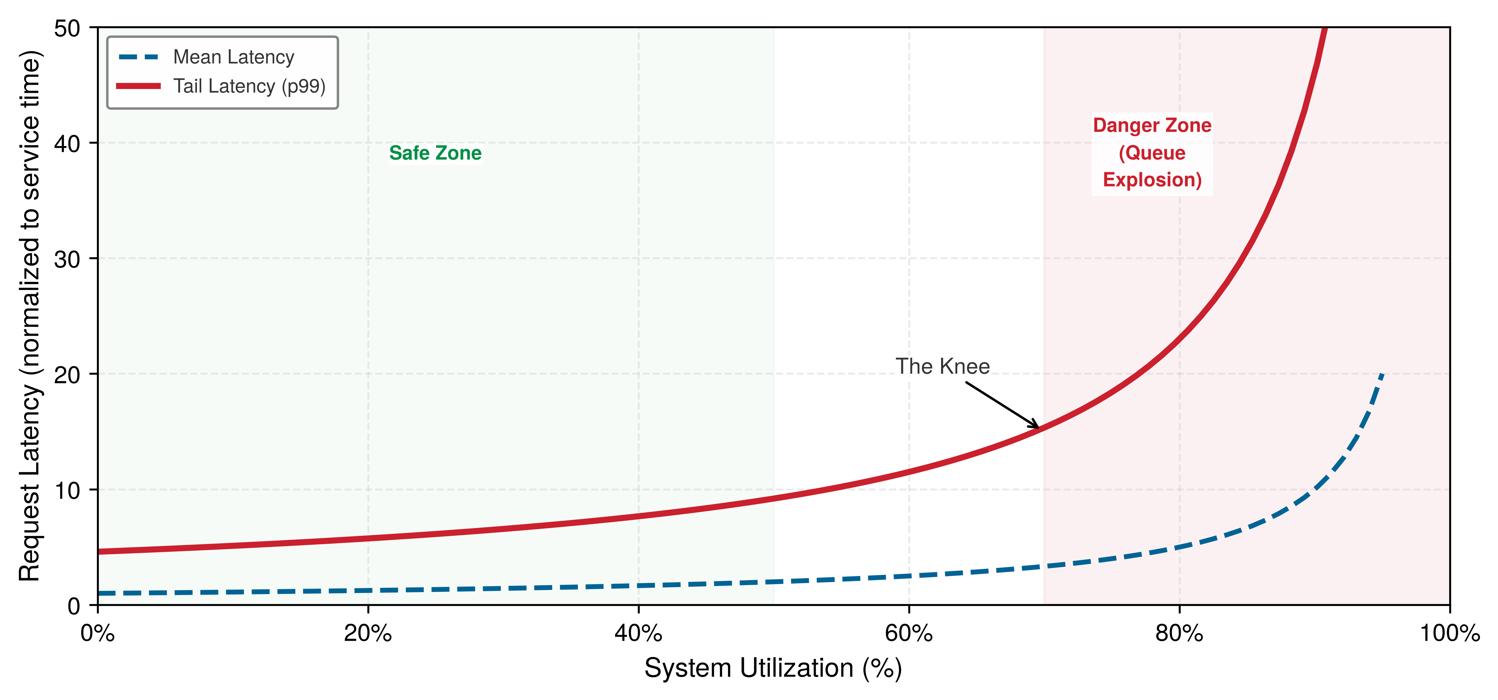
Online serving systems may receive variable, unbatched request streams while still needing predictable response times across diverse physical environments. When a traffic spike exceeds a system’s reserved headroom, performance degrades nonlinearly.
Figure 1 shows that latency remains manageable at moderate utilization and then rises rapidly as the system approaches saturation; this is why latency-sensitive systems reserve headroom rather than planning for a permanently saturated accelerator. Distributions and the long tail gives a mathematical treatment of long-tailed distributions and explains why high-percentile latency matters when an SLO covers the slowest requests. The curve is a simple queueing approximation intended for intuition rather than a specific workload.
Beyond the technical limits of latency, serving economics have also changed rapidly. As models become more efficient and hardware becomes more specialized, the cost per inference has fallen.1 Facebook’s experience at fleet scale illustrates the magnitude of this serving cost problem.
1 Jevons paradox: William Stanley Jevons observed in 1865 that efficiency improvements in coal-powered steam engines increased total coal consumption by making steam power economically viable for applications previously too costly (Jevons 1865); the same dynamic can apply to AI inference: each 10\(\times\) cost reduction opens application classes that were economically infeasible at the previous price point, expanding aggregate demand by more than the efficiency gain. This is why cheaper inference can increase, not decrease, total GPU fleet demand. Efficiency and demand are often complements in AI, not substitutes.
Jevons, William Stanley. 1865. The Coal Question: An Inquiry Concerning the Progress of the Nation, and the Probable Exhaustion of Our Coal Mines. Macmillan; Co.
Example 1.2: The inference tax at Facebook
Scenario: Production ML serving systems at Meta execute tens of trillions of inferences daily across global user-facing services (Hazelwood et al. 2018).
Diagnosis: Recurring inference serving compute and energy costs dwarf initial offline model training expenses. Live request arrival patterns and strict latency bounds constrain GPU batching.
Systems lesson: Model architectures cheap to train can prove unviable to serve at fleet scale. Production serving infrastructure requires hardware-software co-design to balance tail latency, batch size, and recurring operational total cost of ownership.
Hazelwood, Kim, Sarah Bird, David Brooks, Soumith Chintala, Utku Diril, Dmytro Dzhulgakov, Mohamed Fawzy, et al. 2018. “Applied Machine Learning at Facebook: A Datacenter Infrastructure Perspective.” 2018 IEEE International Symposium on High Performance Computer Architecture (HPCA), 620–29. https://doi.org/10.1109/hpca.2018.00059.
OpenAI. 2023b. Introducing ChatGPT and Whisper APIs.
OpenAI. 2023a. GPT-4.
OpenAI. 2024. GPT-4o Mini: Advancing Cost-Efficient Intelligence.
OpenAI Developer Community. 2024. Announcing GPT-4o in the API.
Anthropic. 2024. Introducing the Next Generation of Claude.
Google Developers Blog. 2024. Gemini 1.5 Flash Price Drop with Tuning Rollout Complete, and More.
DeepSeek. 2024. Introducing DeepSeek-V3.
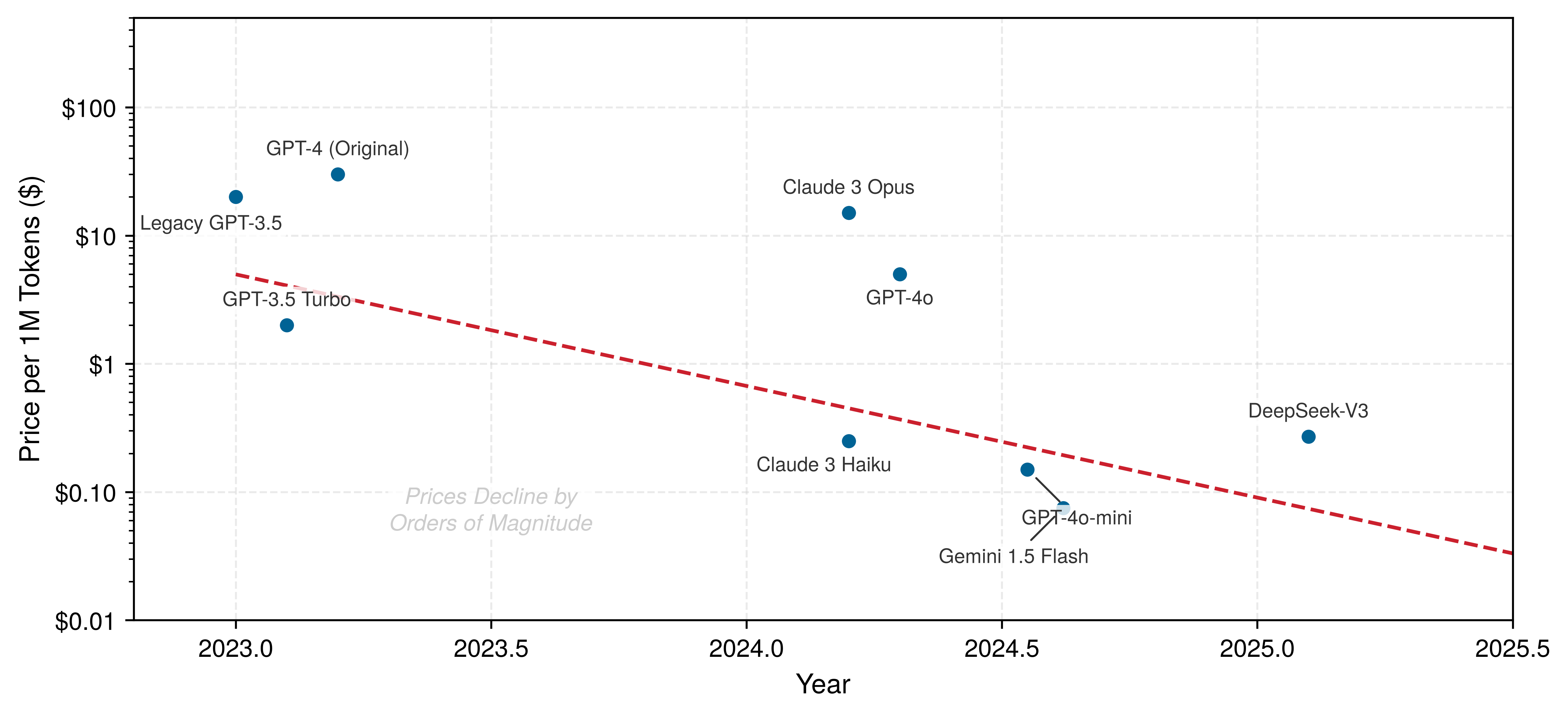
The same serving-economics pressure appears in public API prices. The log-scale price trajectory in figure 2 captures the speed of this cost collapse by tracking representative public API list-price snapshots as a market proxy. Vendor prices change frequently, so these points should be read as historical provenance for the trend rather than as current purchasing guidance (OpenAI 2023b, 2023a, 2024; OpenAI Developer Community 2024; Anthropic 2024; Google Developers Blog 2024; DeepSeek 2024). Each order-of-magnitude drop changes which applications are feasible.
Two pressures now frame the serving problem: tail latency that explodes once utilization passes the queueing knee, and per-inference economics that fall by orders of magnitude as efficiency improves. Together they force a formal definition of serving built around latency rather than throughput.
Definition 1.1: Model serving
Model serving is the operational phase that provides model predictions to end-users or downstream systems under latency, throughput, availability, and cost constraints.
- Significance: Online serving turns training’s throughput priority (\(\eta_{\text{hw}}\)) into a request-latency constraint \((L_{\text{lat}})\), requiring a stack designed around the percentile named by its SLO.
- Distinction: Unlike model training, which commonly processes scheduled batches, serving may handle stochastic online requests, synchronized streams, or offline batches.
- Common pitfall: A frequent misconception is that serving is “just the forward pass.” In reality, it is a systems problem: model execution is only one component of a stack that may include request routing, load balancing, and data transformation.
The SLO2 defines the latency target that shapes every architectural decision in the serving stack, including how the system budgets time across preprocessing, model execution, postprocessing, and transport. When an inference server receives a request, model execution represents only one segment of an end-to-end processing pipeline spanning network transport, serialization, CPU pre/postprocessing, and queue management. Figure 3 shows that raw inputs pass through preprocessing (traditional computing), neural network inference (deep learning), and postprocessing (traditional computing) before producing final outputs. Any of these stages can become the latency bottleneck. Section 1.4.1 quantifies exactly where time goes, revealing a counterintuitive result about which stages dominate.
2 Service level objective (SLO) vs. service level agreement (SLA): An SLO is an internal target (for example, “p99 latency under 50 ms”); an SLA is an external contractual commitment whose violation may carry remedies or penalties. Teams often set SLOs tighter than SLAs to preserve a safety margin. For ML serving, task quality and inference latency can both contribute to SLOs, creating multidimensional targets where improving one dimension (for example, deploying a larger model for accuracy) can violate another (latency).
\begin{tikzpicture}[font=\small\sffamily, >=stealth]
\tikzset{
Box/.style={align=center, inner xsep=2pt,draw=GreenLine, line width=1pt,fill=none,
minimum width=24mm, minimum height=25mm,node distance=1.0},
LineA/.style={BrownLine!70,line width=4.0pt,{-{Triangle[width=1.5*6pt,length=2.0*5pt]}},shorten <=1pt,shorten >=1pt},
ALine/.style={black!50, line width=1.1pt,{{Triangle[width=0.9*6pt,length=1.2*6pt]}-}},
Larrow/.style={fill=violet!50, single arrow,  inner sep=2pt, single arrow head extend=3pt,
            single arrow head indent=0pt,minimum height=10mm, minimum width=3pt}
}
%inbox
\tikzset{%
 pics/inbox/.style = {
        code = {
        \pgfkeys{/channel/.cd, #1}
\begin{scope}[local bounding box=INBOX,scale=\scalefac, every node/.append style={transform shape}]
\node[line width=\Linewidth,draw=\drawcolor,fill=\filllcolor!50,
rectangle,rounded corners=3pt,minimum width=14mm,minimum height=10mm]at(0,0.3){};
\node[line width=\Linewidth,draw=\drawcolor,fill=\filllcolor,
rectangle,rounded corners=3pt,minimum width=15mm,minimum height=10mm]at(0,0.1){};
\node[line width=\Linewidth,draw=\drawcolor,fill=\filllcolor!50,
,rectangle,rounded corners=3pt,minimum width=17mm,minimum height=10mm]
at(0,-0.1){};
\draw[line width=\Linewidth,draw=\drawcolor,fill=\filllcirclecolor,,rounded corners=2pt](-0.92,0.05)--
(-0.92,-0.78)--(0.92,-0.78)--(0.92,0.05)--(0.40,0.05)--(0.32,-0.2)--(-0.29,-0.2)--(-0.40,0.05)--cycle;

\node[single arrow, line width=\Linewidth,draw=black,fill=cyan!90!black!30, rotate=270,
      minimum width = 15pt, single arrow head extend=6pt,
      minimum height=10mm]at(0,0.5) {}; % length of arrow
 \end{scope}
     }
  }
}
%brain
\tikzset{pics/brain/.style = {
        code = {
        \pgfkeys{/channel/.cd, #1}
\begin{scope}[local bounding box=BRAIN,scale=\scalefac, every node/.append style={transform shape}]
\fill[fill=\filllcolor!50](0.1,-0.5)to[out=0,in=180](0.33,-0.5)
to[out=0,in=270](0.45,-0.38)to(0.45,-0.18)
to[out=40,in=240](0.57,-0.13)to[out=110,in=310](0.52,-0.05)
to[out=130,in=290](0.44,0.15)to[out=90,in=340,distance=8](0.08,0.69)
to[out=160,in=80](-0.42,-0.15)to (-0.48,-0.7)to(0.07,-0.7)to(0.1,-0.5)
(-0.10,-0.42)to[out=310,in=180](0.1,-0.5);
\draw[draw=\drawcolor,line width=\Linewidth](0.1,-0.5)to[out=0,in=180](0.33,-0.5)
to[out=0,in=270](0.45,-0.38)to(0.45,-0.18)
to[out=40,in=240](0.57,-0.13)to[out=110,in=310](0.52,-0.05)
to[out=130,in=290](0.44,0.15)to[out=90,in=340,distance=8](0.08,0.69)
(-0.42,-0.15)to (-0.48,-0.7)
(0.07,-0.7)to(0.1,-0.5)
(-0.10,-0.42)to[out=310,in=180](0.1,-0.5);
\draw[fill=\filllcolor,line width=\Linewidth](-0.3,-0.10)to(0.08,0.60)
to[out=60,in=50,distance=3](-0.1,0.69)to[out=160,in=80](-0.26,0.59)to[out=170,in=90](-0.46,0.42)
to[out=170,in=110](-0.54,0.25)to[out=210,in=150](-0.54,0.04)
to[out=240,in=130](-0.52,-0.1)to[out=300,in=240]cycle;
\draw[fill=\filllcolor,line width=\Linewidth]
(-0.04,0.64)to[out=120,in=0](-0.1,0.69)(-0.19,0.52)to[out=120,in=330](-0.26,0.59)
(-0.4,0.33)to[out=150,in=280](-0.46,0.42)
%
(-0.44,-0.03)to[bend left=30](-0.34,-0.04)
(-0.33,0.08)to[bend left=40](-0.37,0.2) (-0.37,0.12)to[bend left=40](-0.45,0.14)
(-0.26,0.2)to[bend left=30](-0.24,0.13)
(-0.16,0.32)to[bend right=30](-0.27,0.3)to[bend right=30](-0.29,0.38)
(-0.13,0.49)to[bend left=30](-0.04,0.51);

\draw[rounded corners=0.8pt,\drawcircle,-{Circle[fill=\filllcirclecolor,length=2.5pt]}](-0.23,0.03)--(-0.15,-0.03)--(-0.19,-0.18)--(-0.04,-0.28);
\draw[rounded corners=0.8pt,\drawcircle,-{Circle[fill=\filllcirclecolor,length=2.5pt]}](-0.17,0.13)--(-0.04,0.05)--(-0.06,-0.06)--(0.14,-0.11);
\draw[rounded corners=0.8pt,\drawcircle,-{Circle[fill=\filllcirclecolor,length=2.5pt]}](-0.12,0.23)--(0.31,0.0);
\draw[rounded corners=0.8pt,\drawcircle,-{Circle[fill=\filllcirclecolor,length=2.5pt]}](-0.07,0.32)--(0.06,0.26)--(0.16,0.33)--(0.34,0.2);
\draw[rounded corners=0.8pt,\drawcircle,-{Circle[fill=\filllcirclecolor,length=2.5pt]}](-0.01,0.43)--(0.06,0.39)--(0.18,0.51)--(0.31,0.4);
\end{scope}
     }
  }
}
%llm
\tikzset{
pics/llm/.style = {
        code = {
        \pgfkeys{/channel/.cd, #1}
\begin{scope}[shift={($(0,0)+(0,0)$)},scale=\scalefac,every node/.append style={transform shape}]
\node[circle,minimum size=12mm,draw=\drawcolor, fill=\filllcolor!70,line width=0.5*\Linewidth](C\picname) at (0,0){};
\def\startangle{90}
\def\radius{1.15}
\def\radiusI{1.1}
\foreach \i [evaluate=\i as \j using \i+1] [count =\k] in {0,2,4,6,8} {
\pgfmathsetmacro{\angle}{\startangle - \i * (360/8)}
\draw[draw=black,-{Circle[black ,fill=\filllcirclecolor,length=5.5pt,line width=0.5*\Linewidth]},line width=1.5*\Linewidth](C\picname)--++(\startangle - \i*45:\radius) ;
\node[circle,draw=black,fill=\filllcirclecolor!80!red!50,inner sep=3pt,line width=0.5*\Linewidth](2C\k)at(\startangle - \j*45:\radiusI) {};
}
\draw[line width=1.5*\Linewidth](2C1)--++(-0.5,0)|-(2C2);
\draw[line width=1.5*\Linewidth](2C3)--++(0.5,0)|-(2C4);
\node[circle,,minimum size=12mm,draw=\drawcolor, fill=\filllcolor!70,line width=0.5*\Linewidth]at (0,0){};
\node[draw,rectangle,rounded corners=1pt,minimum width=7mm,minimum height=4mm,fill=orange!10](R1)at(0.1,0.1){};
\draw[BrownLine,shorten <=2pt,shorten >=2pt ]($(R1.north west)!0.35!(R1.south west)$)--($(R1.north east)!0.35!(R1.south east)$);
\draw[BrownLine,shorten <=2pt,shorten >=2pt ]($(R1.north west)!0.7!(R1.south west)$)--($(R1.north east)!0.7!(R1.south east)$);
\node[draw,rectangle,rounded corners=1pt,minimum width=6mm,minimum height=4mm,fill=orange!10](R2)at(-0.05,-0.15){};
\draw[BrownLine,shorten <=2pt,shorten >=2pt ]($(R2.north west)!0.35!(R2.south west)$)--($(R2.north east)!0.35!(R2.south east)$);
\draw[BrownLine,shorten <=2pt,shorten >=2pt ]($(R2.north west)!0.7!(R2.south west)$)--($(R2.north east)!0.7!(R2.south east)$);
\end{scope}
    }
  }
}
%funnel
\tikzset{%
 pics/funnel/.style = {
        code = {
        \pgfkeys{/channel/.cd, #1}
\begin{scope}[local bounding box=FUNNEL,scale=\scalefac, every node/.append style={transform shape}]
\draw[fill=\filllcolor,line width=\Linewidth,draw=\drawcolor](-0.12,-0.81)--(-0.19,-0.25)--(-0.7,0.41)--(0.7,0.41)--(0.19,-0.25)--(0.12,-0.81)--cycle;
\draw[fill=\filllcolor,line width=\Linewidth,draw=\drawcolor](-0.19,-0.25)--(0.08,-0.25);
\draw[fill=\filllcolor,line width=\Linewidth,draw=\drawcolor](0.16,-0.09)--(0.41,0.31);
%
\node[line width=\Linewidth,draw=\drawcolor,fill=\filllcolor,inner sep=1pt,
rectangle,rounded corners=2pt,minimum width=16mm,minimum height=5pt]at(0,0.5){};
%
\foreach \i in{-0.5,0,0.5}{
\node[single arrow, line width=0.8*\Linewidth,draw=black,fill=\filllcirclecolor, rotate=270,inner sep=1pt,
      minimum width =9pt, single arrow head extend=2pt,
      minimum height=5mm]at(\i,0.9) {}; % length of arrow
   }
\node[single arrow,line width=0.8*\Linewidth,draw=black,fill=\filllcirclecolor, rotate=270,inner sep=1pt,
      minimum width =11pt, single arrow head extend=2pt,
      minimum height=5mm]at(0,-1.1) {}; % length of arrow
 \end{scope}
     }
  }
}
\def\inset{2.0pt} %
\def\myshape{%
  (0,1.34) to[out=220,in=0] (-1.20,1.03) --
  (-1.20,-0.23) to[out=280,in=160] (0,-1.53) to[out=20,in=260] (1.20,-0.23) --
  (1.20,1.03)  to[out=180,in=320] cycle
}
\tikzset{
pics/stitC/.style = {
        code = {
        \pgfkeys{/channel/.cd, #1}
\begin{scope}[shift={($(0,0)+(0,0)$)},scale=\scalefac,every node/.append style={transform shape}]
\fill[fill=\filllcolor!60] \myshape;
%
\begin{scope}
  \clip \myshape;
  \draw[draw=\filllcolor!60, line width=3*\inset,fill=white] \myshape; % Color and thickness as desired
\end{scope}
\draw[red,line width=3pt](-0.7,-0.35)--++(320:0.5)--++(50:1.5);
\end{scope}
    }
  }
}
%gear-arrow
% #1 number of teeths
% #2 radius intern
% #3 radius extern
% #4 angle from start to end of the first arc
% #5 angle to decale the second arc from the first
% #6 inner radius to cut off
\tikzset{
  pics/gearAR/.style args={#1/#2/#3/#4/#5/#6/#7}{
   code={
           \pgfkeys{/channel/.cd, #7}
\begin{scope}[shift={($(0,0)+(0,0)$)},scale=\scalefac,every node/.append style={transform shape},
LinE/.style={\filllcirclecolor,line width=5.0pt,
{{Triangle[width=1.5*10pt,length=2.0*5pt]}-},shorten <=5pt,shorten >=1pt},
ELin/.style={\filllcirclecolor,line width=7.0pt,
{-{Triangle[width=1.15*10pt,length=2.0*5pt]}},shorten <=0pt,shorten >=0pt}]
    \pgfmathtruncatemacro{\N}{#1}%,
    \def\rin{#2}\def\rout{#3}\def\aA{#4}\def\aOff{#5}\def\rcut{#6}%
    \path[rounded corners=0.5pt,draw=\drawcolor,fill=\filllcolor]
      (0:\rin)
      \foreach \i [evaluate=\i as \n using (\i-1)*360/\N] in {1,...,\N}{%
        arc (\n:\n+\aA:\rin)
        -- (\n+\aA+\aOff:\rout)
        arc (\n+\aA+\aOff:\n+360/\N-\aOff:\rout)
        -- (\n+360/\N:\rin)
      } -- cycle;
      \draw[draw=none,fill=white](0,0) circle[radius=\rcut];
\draw[ELin](0,0)--++(0:2.5);
\end{scope}
  }}
}
%testing+pencil
\tikzset{
pics/testing/.style = {
        code = {
        \pgfkeys{/channel/.cd, #1}
\begin{scope}[local bounding box=TESTING1,shift={($(0,0)+(0,0)$)},scale=\scalefac,every node/.append style={transform shape}]
\newcommand{\tikzxmark}{%
\tikz[scale=0.18] {
    \draw[line width=0.7,line cap=round,RedLine] (0,0) to [bend left=6] (1,1);
    \draw[line width=0.7,line cap=round,RedLine] (0.2,0.95) to [bend right=3] (0.8,0.05);
}}
\newcommand{\tikzxcheck}{%
\tikz[scale=0.16] {
    \draw[line width=0.7,line cap=round,GreenLine] (0.5,0.75)--(0.85,-0.1) to [bend left=16] (1.5,1.55);

}}
 \node[draw, minimum width  =15mm, minimum height = 20mm, inner sep = 0pt,
        rounded corners,draw = \drawcolor, fill=\filllcolor!10, line width=\Linewidth](COM){};
\node[draw=GreenLine,inner sep=4pt,fill=white](CB1) at ($(COM.north west)!0.25!(COM.south west)+(0.3,0)$){};
\node[xshift=0pt]at(CB1){\tikzxcheck};
\node[draw=RedLine,inner sep=4pt,fill=white](CB2) at ($(COM.north west)!0.5!(COM.south west)+(0.3,0)$){};
\node[xshift=0pt]at(CB2){\tikzxmark};
\node[draw=RedLine,inner sep=4pt,fill=white](CB3) at ($(COM.north west)!0.75!(COM.south west)+(0.3,0)$){};
\node[xshift=0pt]at(CB3){\tikzxmark};
\draw[GreenLine,decoration={zigzag,segment length=4pt, amplitude=0.5pt},decorate]($(CB1)+(0.3,0.05)$)--++(0:0.8);
\draw[GreenLine,decoration={zigzag,segment length=4pt, amplitude=0.5pt},decorate]($(CB1)+(0.3,-0.12)$)--++(0:0.7);
\draw[RedLine,decoration={zigzag,segment length=4pt, amplitude=0.5pt},decorate]($(CB2)+(0.3,0.05)$)--++(0:0.8);
\draw[RedLine,decoration={zigzag,segment length=4pt, amplitude=0.5pt},decorate]($(CB2)+(0.3,-0.12)$)--++(0:0.6);
\draw[RedLine,decoration={zigzag,segment length=4pt, amplitude=0.5pt},decorate]($(CB3)+(0.3,0.05)$)--++(0:0.8);
\draw[RedLine,decoration={zigzag,segment length=4pt, amplitude=0.5pt},decorate]($(CB3)+(0.3,-0.12)$)--++(0:0.6);
\end{scope}
    }
  }
}
%pencil
\tikzset{
pics/pencil/.style = {
        code = {
        \pgfkeys{/channel/.cd, #1}
\begin{scope}[local bounding box=TESTING1,shift={($(0,0)+(0,0)$)},scale=\scalefac,every node/.append style={transform shape},rotate=340]
            \fill[fill=\filllcolor!70] (0,4) -- (0.4,4) -- (0.4,0) --(0.3,-0.15) -- (0.2,0) -- (0.1,-0.14) -- (0,0) -- cycle;
            \draw[color=white,thick] (0.2,4) -- (0.2,0);
            \fill[black] (0,3.5) -- (0.2,3.47) -- (0.4,3.5) -- (0.4,4) arc(30:150:0.23cm);
            \fill[fill=\filllcolor!40] (0,0) -- (0.2,-0.8)node[coordinate,pos=0.75](a){} -- (0.4,0)node[coordinate,pos=0.25](b){} -- (0.3,-0.15) -- (0.2,0) -- (0.1,-0.14) -- cycle;
            \fill[fill=\filllcolor] (a) -- (0.2,-0.8) -- (b) -- cycle;

\end{scope}
    }
  }
}
\pgfkeys{
  /channel/.cd,
   Depth/.store in=\Depth,
  Height/.store in=\Height,
  Width/.store in=\Width,
  filllcirclecolor/.store in=\filllcirclecolor,
  filllcolor/.store in=\filllcolor,
  drawcolor/.store in=\drawcolor,
  drawcircle/.store in=\drawcircle,
  scalefac/.store in=\scalefac,
  Linewidth/.store in=\Linewidth,
  picname/.store in=\picname,
  filllcolor=BrownLine,
  filllcirclecolor=violet!20,
  drawcolor=black,
  drawcircle=violet,
  scalefac=1,
  Linewidth=0.5pt,
  Depth=1.3,
  Height=0.8,
  Width=1.1,
  picname=C
}
%Raw Data
\node[Box](B1){};
\fill[cyan!07](B1.north west) rectangle ($(B1.north east)!0.6!(B1.south east)$)coordinate(B1DE);
\fill[cyan!20](B1.south east) rectangle ($(B1.north west)!0.6!(B1.south west)$)coordinate(B1LE);
\node[Box,draw=BlueD](){};
\tikzset{Text2/.style={font=\sffamily\bfseries\small,align=center}}
\node[Text2]at($(B1.south west)!0.5!(B1DE)$){Raw Data};
\coordinate(Q1)at($(B1.north west)!0.5!(B1DE)$);
\pic[shift={(0,0)}] at  (Q1){inbox={scalefac=0.7,picname=1,Linewidth=1.0pt,
 filllcolor=BrownL,drawcolor=black,filllcirclecolor=orange!70!yellow!80}};
%Pre-processing
\node[Box, right=0.75 of B1](B2){};
\fill[cyan!07](B2.north west) rectangle ($(B2.north east)!0.6!(B2.south east)$)coordinate(B2DE);
\fill[cyan!20](B2.south east) rectangle ($(B2.north west)!0.6!(B2.south west)$)coordinate(B2LE);
\node[Box, right=0.75 of B1,draw=BlueD](B2){};
\node[Text2]at($(B2.south west)!0.5!(B2DE)$){Pre-\\processing};
\coordinate(Q2)at($(B2.north west)!0.5!(B2DE)$);
\pic[shift={(0,0)}] at  (Q2){funnel={scalefac=0.53,picname=1,Linewidth=0.5pt,
 filllcolor=green!70!orange!70,drawcolor=black,filllcirclecolor=red!70!blue!80}};
%Neural Network
\node[Box, right=of B2](B3){};
\fill[green!07](B3.north west) rectangle ($(B3.north east)!0.6!(B3.south east)$)coordinate(B3DE);
\fill[green!20](B3.south east) rectangle ($(B3.north west)!0.6!(B3.south west)$)coordinate(B3LE);
\node[Box, right=of B2,draw=GreenD](B3){};
\node[Text2]at($(B3.south west)!0.5!(B3DE)$){Neural\\ Network};
\coordinate(Q3)at($(B3.north west)!0.5!(B3DE)$);
%\pic[shift={(0,0)}] at  (Q3){brain={scalefac=0.9,picname=1,filllcolor=orange!30!, Linewidth=0.95pt}};
\pic[shift={(0,0)}] at  (Q3){llm={scalefac=0.6,drawcolor=BlueLine,filllcolor=BlueLine!50!, Linewidth=1pt,filllcirclecolor=red}};
%Raw output
\node[Box, right=of B3](B4){};
\fill[violet!07](B4.north west) rectangle ($(B4.north east)!0.6!(B4.south east)$)coordinate(B4DE);
\fill[violet!20](B4.south east) rectangle ($(B4.north west)!0.6!(B4.south west)$)coordinate(B4LE);
\node[Box, right=of B3,draw=VioletLine](B4){};
\node[Text2]at($(B4.south west)!0.5!(B4DE)$){Raw\\ Output};
\coordinate(Q4)at($(B4.north west)!0.5!(B4DE)$);
 \pic[shift={(0,0)}] at (Q4) {gearAR={14/1.4/1.8/8/4/0.7/scalefac=0.35,drawcolor=BlueLine,filllcolor=BlueLine,filllcirclecolor=red}};
%Post-processing
\node[Box, right=0.75 of B4](B5){};
\fill[violet!05](B5.north west) rectangle ($(B5.north east)!0.6!(B5.south east)$)coordinate(B5DE);
\fill[violet!15](B5.south east) rectangle ($(B5.north west)!0.6!(B5.south west)$)coordinate(B5LE);
\node[Box, right=0.75 of B4,draw=VioletLine](B5){};
\node[Text2]at($(B5.south west)!0.5!(B5DE)$){Post-\\processing};
\coordinate(Q5)at($(B5.north west)!0.5!(B5DE)$);
\pic[shift={(0,0)}] at  (Q5){testing={scalefac=0.65,picname=1,drawcolor=myblue,filllcolor=myblue, Linewidth=1.0pt}};
\pic[shift={(0,-0.5)},rotate=-15] at  (Q5){pencil={scalefac=0.30,picname=1,filllcolor=mygreen, Linewidth=1.0pt}};
%%%%%%
%Final output
\node[Box, right=0.75 of B5](B6){};
\fill[violet!05](B6.north west) rectangle ($(B6.north east)!0.6!(B6.south east)$)coordinate(B6DE);
\fill[violet!15](B6.south east) rectangle ($(B6.north west)!0.6!(B6.south west)$)coordinate(B6LE);
\node[Box, right=0.75 of B5,draw=VioletLine]{};
\node[Text2]at($(B6.south west)!0.5!(B6DE)$){Final Output};
\coordinate(Q6)at($(B6.north west)!0.5!(B6DE)$);
\pic[shift={(0,0.05)}] at  (Q6){stitC={scalefac=0.45,drawcolor=orange,filllcolor=green!55!black}};
%arrows
\foreach \i in{1,2,3,4,5}{
\pgfmathtruncatemacro{\X}{\i + 1} %
\draw[LineA](B\i)--(B\X);
}
\node[draw=myblue,line width=0.75pt,fit=(B1)(B2),inner ysep=3mm,inner xsep=4mm,xshift=1mm](F1){};
\node[draw=none,fit=(B3),inner ysep=3mm,inner xsep=4mm](F2){};
\node[draw=mypurple,line width=0.75pt,fit=(B4)(B6),inner ysep=3mm,inner xsep=4mm,xshift=-1mm](F3){};
\node[below =0pt of F1,text=myblue]{Pre-processing};
\node[below =0pt of F2,text=GreenD]{Deep Learning};
\node[below =0pt of F3,text=mypurple]{Post-processing};

\end{tikzpicture}The pipeline turns serving into an orchestration problem: preprocessing, model execution, postprocessing, and transport all compete for the same latency budget. Before optimizing any one stage, the system must decide whether predictions are computed ahead of time or on demand.
Static vs. dynamic inference
Before optimizing how to reduce inference latency, the system must decide when predictions are computed. An early architectural decision is whether predictions happen before or during user requests (Google 2024). This choice shapes system design, cost structure, and capability boundaries.
Google. 2024. Static Vs. Dynamic Inference. Google Machine Learning Crash Course.
Static inference
Static inference (also called offline or batch inference) precomputes predictions for anticipated inputs and stores them for retrieval. Consider a recommendation system that generates predictions for all user-item pairs nightly. When a user requests recommendations, the system retrieves precomputed results from a lookup table rather than running inference. This approach moves compute out of the request path, enables offline quality checks, and can reduce serving costs for predictable inputs. However, static inference needs either a fallback online path or a refreshed batch computation when requests include unanticipated inputs or newly updated models.
Dynamic inference
Dynamic inference (also called online or real-time inference) computes predictions on demand when requests arrive. This can handle previously unseen inputs within the service’s supported schema and reflects a new model version once that version is deployed. The cost is a live latency budget that constrains model complexity and demands robust monitoring infrastructure.
Example 1.3: The cost of latency
Latency constraints directly dictate infrastructure costs. Consider a GPU server renting for $4/hour.
Scenario A (low latency): Batch size 1.
- Latency: 5 ms.
- Throughput: 200 req/s.
- Cost per million queries: $5.56.
Scenario B (high throughput): Batch size 8.
- Latency: 10 ms (doubled due to batching overhead).
- Throughput: 800 req/s (quadrupled due to parallel efficiency).
- Cost per million queries: $1.39.
Systems insight: Reducing latency from 10 ms to 5 ms increases the hardware bill by 300 percent. Engineers must quantify whether that speedup generates enough business value to justify the 4× cost increase.
For our ResNet-50 image classifier, consider two deployment scenarios. A static approach suits a photo organization app that preclassifies all images in a user’s library overnight. With 10,000 photos and 5 ms inference each, batch processing takes ~50 s total, and users see instant classification when browsing. A dynamic approach suits a content moderation API that must classify user-uploaded images in real-time, with each image requiring the full preprocessing→inference→postprocessing pipeline and a 100 ms latency budget. A production image-classification system can combine the approaches: frequently requested images, such as popular products or known memes, are preclassified and cached, while novel uploads trigger dynamic inference.
The choice between static and dynamic serving has direct economic implications. A stricter latency requirement can raise infrastructure costs when it requires smaller batches, additional replicas, or more capable hardware. Quantifying this trade-off in dollar terms reveals whether the latency reduction justifies that premium.
Many production systems combine both approaches. Common queries can hit a cache populated by batch inference while uncommon requests trigger dynamic computation. Understanding this spectrum matters because it determines which subsequent optimization strategies apply. Static inference optimizes for throughput during batch computation and storage efficiency for serving. Dynamic inference optimizes for per-request latency under concurrent load, which requires understanding where time goes within each request.
The static-vs.-dynamic decision is the first of several architectural choices that shape serving system design. Equally important is where the model executes, since deployment context constrains every subsequent optimization.
All of the cost analysis in this section assumes a traditional forward pass: a fixed computation graph that executes once per request and produces a result. A new class of models upends that assumption by deliberately increasing the amount of computation spent per query, trading latency for answer quality, and the serving cost implications are substantial.
Systems Perspective 1.1: Looking ahead: Spending more compute per query
Traditional serving optimizes for minimizing latency \((L_{\text{lat}} \to 0)\). Here, the optimization target expands to include answer quality. Some inference-time-compute systems deliberately spend more compute cycles to improve answer quality. Token generation is often memory-bandwidth bound at small batches, but larger batches or long contexts can shift the bottleneck toward compute or KV-cache traffic. These systems may generate far more tokens per request, including intermediate reasoning or search tokens, increasing the total compute and energy spent per query.
Whether a system spends one forward pass or many reasoning steps per query, deployment context still determines the feasible latency and cost envelope. That context is the next variable.
The spectrum of serving architectures
Although “serving” often implies a networked server processing API requests, the architectural pattern varies by deployment environment. Deployment Paradigm Framework introduced the four deployment paradigms (Cloud, Edge, Mobile, and TinyML) and the physical constraints (the light barrier, the power wall, and the memory wall) that give rise to them. Architecturally, serving spans a continuum from centralized networked microservices (which pool accelerators to optimize throughput and cost-per-query at the expense of network round-trip overhead and cold-start latency) to application-embedded edge serving (which run models inside client processes via direct function calls, eliminating network latency and preserving privacy at the expense of strict device memory and power constraints). Those constraints do not disappear at serving time; serving adds latency SLOs and cost pressure on top of hardware limits that training could absorb through patience. The same model may require different serving strategies depending on where it executes.
Networked serving (cloud/data center)
In networked serving, the model runs as a standalone service (microservice), matching the cloud deployment paradigm that Cloud ML: Computational Power characterized as trading latency for larger pooled compute. The primary interface is the network through protocols such as HTTP or gRPC, so network transfer and serialization join model execution as possible binding constraints. Data-center hardware such as NVIDIA GPUs (V100, A100, H100), Google Tensor Processing Units (TPUs), and AWS Inferentia supports high-throughput batching and concurrency, but cold start can still stretch from seconds to minutes because container startup, model loading, and warmup sit outside the steady-state inference path.
Application-embedded serving (mobile/edge)
In application-embedded serving, the model runs within the user application process (for example, a smartphone app using CoreML or TensorFlow Lite), following the embedded paradigm that Edge ML: Latency and Privacy and Mobile ML: Offline Intelligence analyzed for its latency, privacy, and offline advantages. There is no “server.” The interface is a function call, so optimization focuses on energy and responsiveness (SingleStream) rather than shared-server throughput.
An important advantage is zero-copy inference: when data moves through a system, each copy consumes CPU cycles and memory bandwidth. In cloud serving, a camera frame might pass from a network buffer to application memory, a preprocessing buffer, GPU-accessible host memory, and finally accelerator memory. A mobile pipeline can remove some of these copies when its camera, image signal processor, CPU, and NPU exchange compatible shared buffers. This reduces latency and energy, although preprocessing or format conversion may still involve the CPU or image signal processor. The mechanism requires coordinated hardware and software support, as in unified-memory system-on-chip designs such as Apple A- and M-series processors and Qualcomm Snapdragon.
Typical hardware includes mobile NPUs (Apple Neural Engine, Qualcomm Hexagon) and embedded GPUs (Jetson). When the model is already resident and compiled, startup can be measured in milliseconds; first inference may take much longer if it triggers loading or just-in-time compilation. Mobile power and thermal envelopes are device-specific, and prolonged inference can trigger throttling.
Bare-metal serving (TinyML)
In TinyML serving, the model is commonly compiled into microcontroller firmware, reaching the extreme end of the deployment spectrum that TinyML: Ubiquitous Sensing introduced as ubiquitous sensing at microwatt power budgets. Many deployments have no general-purpose operating system or runtime allocator; “serving” is a tight loop that reads sensors and invokes an interpreter. Optimization focuses on fitting weights and preallocated working memory, such as a Tensor Arena, in static random-access memory (SRAM), and request batching is generally infeasible. Typical hardware includes ARM Cortex-M series, ESP32, and specialized TinyML accelerators. Startup can be extremely short when weights remain in flash and working memory is preallocated, while the power budget ranges from microwatts to milliwatts for battery operation over months or years.
The deployment tiers differ first in their operating envelopes. Table 1 compares the latency, batch, memory, power, update, failure, and monitoring constraints that follow from each environment.
| Characteristic | Cloud/Data center | Mobile/Edge | TinyML |
|---|---|---|---|
| Latency Target | 10–100 ms | 20–50 ms | 1–100 ms |
| Batch Size | 1–128 (dynamic) | 1 (fixed) | 1 (fixed) |
| Memory | 16–80 GB VRAM | 2–8 GB shared | 256 KB–2 MB SRAM |
| Power | 300–700 W | 1–10 W | 1–100 mW |
| Update Mechanism | Container deploy | App store update | Firmware over-the-air (OTA) |
| Failure Mode | Retry/failover | Graceful degradation | Silent or reset |
| Monitoring | Full telemetry | Limited analytics | Heartbeat only |
Systems Perspective 1.2: ResNet-50 across the serving spectrum
Systems insight: The “same model” claim is misleading: the cloud and mobile tiers share the ResNet-50 graph but use different precision and runtimes, while the TinyML tier cannot run ResNet-50 and substitutes an architecture designed for its constraints. Treating these as one model hides the work that makes each deployment possible.
Applying those envelopes to one image-classification workload, table 2 shows why cloud and mobile can adapt ResNet-50 while TinyML must substitute MobileNetV2.
| Dimension | Cloud | Mobile | TinyML |
|---|---|---|---|
| Model format | TensorRT FP16 engine | TensorFlow Lite INT8 | Not feasible (25.6 MB); alternative: MobileNetV2 INT8 (3.5 MB) |
| Inference (batch-1) | 1.4 ms (batch-16: 14 ms) | 12 ms (NPU), 45 ms (CPU) | 120 ms |
| Throughput | 1,143 img/s (batched) | ~80 img/s (single-stream) | ~8 img/s |
| Memory | 2 GB VRAM (batch-32) | 150 MB peak (shared with app) | 320 KB arena (fits in 512 KB SRAM) |
| Energy/inference | — | 0.8 mJ (NPU), 4.2 mJ (CPU) | 12 mJ |
The load balancer layer
When traffic exceeds what a single machine can handle, cloud and data center deployments that run multiple replicas of the same model require an additional infrastructure layer: the load balancer. Production serving systems place load balancers between clients and model servers, providing three essential functions for serving infrastructure.
Request distribution, the first function, routes incoming requests to available model replicas using algorithms like round-robin or least-connections. For latency-sensitive ML serving, algorithms that route away from slow or overloaded replicas improve tail latency. The second, health monitoring, continuously verifies that replicas are ready to serve, routing traffic away from unhealthy instances. For ML systems, health checks must verify both process liveness and model readiness, confirming that weights are loaded and warmup is complete. The third, deployment support, enables safe model updates by gradually shifting traffic between versions instead of treating release as an all-at-once switch. Model deployment later turns that basic traffic-shift idea into full deployment and validation strategies.
For single-machine serving with multiple model instances, such as running several Open Neural Network Exchange (ONNX) Runtime sessions, the framework and operating system handle request queuing. The full complexity of load balancing becomes necessary when scaling to distributed inference systems, where multiple machines serve the same model. The implementation details of request distribution algorithms and multi-replica architectures belong to that distributed context.
When capacity planning considers “the server” in this single-machine serving analysis, it means the machine’s model serving capacity. The queuing dynamics analyzed in section 1.5 apply to understanding single-machine behavior and determining when scaling to multiple machines becomes necessary.
While load balancers distribute requests across replicas, achieving predictable latency also requires controlling what happens within each machine. The operating system environment introduces its own sources of variability.
Deterministic latency and resource isolation

One noisy neighbor perturbs every workload sharing the node.
An inference server does not operate in isolation. On a single machine, the operating system manages multiple competing processes (logging agents, monitoring tools, and system interrupts) that can intermittently steal CPU cycles from the inference pipeline. These “noisy neighbors” are a primary source of latency jitter, where the time required to process identical requests varies significantly, causing the 99th percentile (p99) latency to spike even when the hardware is underused. Resource contention can therefore widen tail latency through service-time jitter, a different mechanism from the utilization-driven queue growth in figure 1.
Achieving deterministic performance on a single node requires reducing interference from the operating system’s normal resource-sharing behavior. Predictable serving systems such as Clockwork show that deep neural network (DNN) inference can meet tight request-level SLOs when scheduling and execution are controlled carefully (Gujarati et al. 2020). CPU affinity (pinning) is one local isolation tool: it restricts the inference server’s threads to specific physical cores so latency-sensitive work is less exposed to thread migration and cache-locality loss. Pinning can reduce one source of latency jitter, but it is part of a broader resource-isolation strategy rather than a complete solution.
Memory locking (mlock) addresses a related but distinct source of jitter. By default, the OS can page eligible host memory regions to disk under memory pressure. If the CPU or GPU’s direct memory access (DMA) engine accesses a region that has been paged out, the transfer stalls until the data is faulted back into RAM. Locking host-resident weights, staging buffers, or an offloaded KV cache prevents these stalls, though locked pages cannot be reclaimed by other processes. mlock does not lock accelerator high-bandwidth memory (HBM).
The third technique, interrupt shielding, completes the isolation picture. Network and storage interrupts routed to inference cores can preempt GPU command submission at unpredictable moments. Steering these interrupts to noninference cores ensures that bursts of incoming traffic do not disrupt the GPU’s command stream, which is particularly important for maintaining stable tail latency under load.
These isolation principles transform a simple “model script” into a deterministic service, a transition essential for safety-critical applications like autonomous driving or real-time industrial control. The deployment spectrum, load balancing, and resource isolation define where models serve and what infrastructure supports them. The remaining question is how the serving software itself is organized, specifically what components comprise an inference server and how they coordinate to turn irregular user traffic into efficient hardware utilization.
Self-Check: Question
An e-commerce platform evaluates precomputing product recommendations offline (static inference) versus computing them on demand when a user visits the homepage (dynamic inference). Which trade-off correctly characterizes static inference compared to dynamic inference?
- Static inference eliminates database storage costs but increases real-time p99 latency by executing large batched matrix multiplications during user page loads.
- Static inference guarantees real-time contextual adaptation to intra-session user clicks but requires dedicated high-end GPUs on the critical request path.
- Static inference trades storage capacity and potential prediction staleness for predictable sub-millisecond retrieval latency, whereas dynamic inference provides fresh predictions from live context at the expense of computational latency and variable serving capacity.
- Static inference requires running unbatched single-sample inferences across microcontrollers, whereas dynamic inference processes large offline shards across cloud clusters.
Why does bare-metal TinyML serving on microcontrollers (e.g., ARM Cortex-M) preclude the use of standard cloud serving frameworks (like Triton or vLLM), and what architectural adaptations are required?
True or False: Under a simple \(M/M/1\) queueing model approximation, when server utilization (\(\rho_{\text{serv}}\)) reaches 90%, the 99th percentile (p99) tail latency is approximately equal to 1.5 times the mean latency.
To prevent OS scheduler thread migration and cross-socket memory bus contention from causing latency jitter on multi-socket CPU serving nodes, engineers bind worker threads to specific processor cores and local memory nodes using the ____ utility.
A high-throughput model serving cluster sits behind a Layer 7 load balancer. Which routing algorithm is best suited for minimizing p99 tail latency when inference execution times vary significantly across requests due to variable input sequence lengths?
- Peak exponentially weighted moving average (Peak-EWMA) or least-pending-requests routing, which steers traffic away from replicas currently processing long-running requests.
- Static round-robin routing, which deterministically rotates incoming connections across all healthy replicas regardless of current queue depths.
- Random routing with hash-based sticky IP assignment, which pins client IP addresses permanently to specific backends without monitoring load.
- Maximum-throughput greedy allocation, which concentrates all incoming traffic onto a single primary replica until its memory is completely saturated before spilling over.
Serving System Architecture
User requests arrive in unpredictable bursts, one millisecond apart, then five seconds of silence, while accelerators demand steady, uniformly-sized batches. Bridging this gap requires more than a Python script calling model.predict(); it requires a specialized software architecture that absorbs traffic variability, forms efficient batches, and keeps hardware saturated without violating latency SLOs.
Internal architecture and request flow
Model optimization focuses on the mathematical artifact, while model serving requires a specialized software architecture to manage high-frequency request streams and hardware utilization. An inference server3 (such as NVIDIA Triton or TensorFlow Serving) is not a simple wrapper around a model script; it is a high-performance scheduler that manages concurrency, memory, and data movement.
3 Inference server: Google’s TensorFlow Serving (Olston et al. 2017) helped establish the separation of model logic from serving infrastructure; NVIDIA’s Triton (NVIDIA 2024b) extends this pattern across multiple model frameworks and backends. The critical design insight is that a scheduler and dynamic batcher turn irregular single-request traffic into accelerator-friendly execution, improving utilization when latency budgets allow batching. Exact utilization gains depend on model, hardware, arrival rate, and the configured batching window.
Olston, Christopher, Noah Fiedel, Kiril Gorovoy, Jeremiah Harmsen, Li Lao, Fangwei Li, Vinu Rajashekhar, Sukriti Ramesh, and Jordan Soyke. 2017. “TensorFlow-Serving: Flexible, High-Performance ML Serving.” CoRR abs/1712.06139. https://doi.org/10.48550/arXiv.1712.06139.
NVIDIA. 2024b. NVIDIA Triton Inference Server.
The internal anatomy of these servers reveals how they bridge the gap between irregular user traffic and the highly regular, batch-oriented requirements of accelerators. Every request traverses a multi-stage pipeline designed to maximize hardware throughput while minimizing latency overhead. Figure 4 separates the six stages so each component’s role in absorbing traffic, queueing, batching, and accelerator execution is explicit.
\begin{tikzpicture}[font=\small\sffamily]
  \tikzset{
    Box/.style={draw=none,minimum width=20mm, minimum height=15mm, node distance=18mm},
    Arr/.style={-{Triangle[width=10pt,length=8pt]}, line width=5pt,cyan!40,shorten >=1pt, shorten <=2pt},
 Box2/.style={align=flush center, inner xsep=2pt,draw=OrangeLine,
  font=\fontsize{7pt}{9}\sffamily,
    line width=0.75pt, rounded corners,fill=OrangeL!30, text width=16mm,
    minimum width=16mm, minimum height=9mm},
LineA/.style = {violet!60,{Circle[line width=1.0pt,fill=white,length=5.5pt]}-,line width=1.5pt,shorten <=-3pt}
}
%laptop
\tikzset{
pics/laptop/.style = {
        code = {
        \pgfkeys{/channel/.cd, #1}
\begin{scope}[shift={($(0,0)+(0,0)$)},scale=\scalefac,every node/.append style={transform shape}]
\node[rounded corners=2pt,rectangle,minimum width=60,minimum height=37,
fill=\filllcolor!60,line width=\Linewidth,draw=black](EKV)at(0,0.53){};
%
\node[draw=black,rounded corners=2pt,rectangle,minimum width=53,minimum height=30,
fill=\filllcolor!10,line width=\Linewidth,](EK)at(0,0.53){};
\coordinate(SM1)at($(EK.south west)+(0.15,0.5)$);
\coordinate(SM2)at($(EK.south east)+(-1.1,0.5)$);
\coordinate(OK1)at($(EK.220)+(0,0.7)$);
\coordinate(OK2)at($(EK.240)+(0,0.7)$);
\node[fill=black,inner sep=0pt,ellipse,minimum width=2pt,minimum height=3pt](OKO1)at(OK1){};
\node[fill=black,inner sep=0pt,ellipse,minimum width=2pt,minimum height=3pt](OKO2)at(OK2){};
\draw[line width=1.4pt](SM1)to [bend right=45](SM2);
%%
\coordinate(4BL)at($(EK.south west)+(0.95,0.3)$);
    \def\n{5}          % broj boksova
    \def\w{0.12}        % širina boksa (mm)
    \def\h{0.5}       % visina boksa (mm)
    \def\gap{0.05}      % razmak između boksova (mm)
    % niz boksova
    \foreach \i in {0,...,4} {
      \pgfmathsetmacro{\x}{\i*(\w+\gap)}
      % popuna (klipujemo unutar ivica)
      \begin{scope}
        \clip[] ($(4BL)+(\x,0)$) rectangle ++(\w,\h);
        \fill[gray!10]($(4BL)+(\x,0)$) rectangle ++(\w,\h*1);
        \fill[fill=\filllcirclecolor]($(4BL)+(\x,0)$) rectangle ++(\w,\h*\Level);
      \end{scope}
      % kontura preko
      \draw[line width=0.6pt,draw=black]($(4BL)+(\x,0)$)  rectangle ++(\w,\h);
    }
%
\draw[fill=\filllcolor!60!black!30,line width=\Linewidth](-1.00,-0.1)--(1.0,-0.1)--(1.28,-0.6)--(-1.28,-0.6)--cycle;
\draw[fill=\filllcolor!60!black!30,line width=\Linewidth](1.28,-0.6)--(-1.28,-0.6)arc[start angle=180, end angle=270, radius=4pt]--(1.14,-0.73)
arc[start angle=270, end angle=355, radius=4pt]--cycle;
\draw[fill=\filllcolor!30!black!10,line width=\Linewidth](-0.95,-0.17)--(0.95,-0.17)--(1.03,-0.34)--(-1.03,-0.34)--cycle;
\draw[fill=\filllcolor!30!black!20,line width=\Linewidth](-0.16,-0.52)--(0.16,-0.52)--(0.14,-0.42)--(-0.14,-0.42)--cycle;
\end{scope}
    }
  }
}

\tikzset {
pics/gatewey/.style = {
        code = {
        \pgfkeys{/channel/.cd, #1}
\begin{scope}[local bounding box=GAT,scale=\scalefac, every node/.append style={transform shape}]
\def\rI{4mm}
\def\rII{2.8mm}
\def\rIII{1.6mm}
\draw[draw=\drawcolor,line width=0.8*\Linewidth](0,0)--(0,0.38)--(1.2,0.38)--(1.2,0)--cycle;
\draw[draw=\drawcolor,line width=\Linewidth](0.6,0.4)--(0.6,0.9);

 \draw[draw=\drawcolor, line width=\Linewidth] (0.6,0.9)+(60:\rI) arc[start angle=60, end angle=-60, radius=\rI];
\draw[draw=\drawcolor, line width=\Linewidth] (0.6,0.9)+(50:\rII) arc[start angle=50, end angle=-50, radius=\rII];
\draw[draw=\drawcolor, line width=\Linewidth] (0.6,0.9)+(30:\rIII) arc[start angle=30, end angle=-30, radius=\rIII];
%
 \draw[draw=\drawcolor, line width=\Linewidth] (0.6,0.9)+(120:\rI) arc[start angle=120, end angle=240, radius=\rI];
\draw[draw=\drawcolor, line width=\Linewidth] (0.6,0.9)+(130:\rII) arc[start angle=130, end angle=230, radius=\rII];
\draw[draw=\drawcolor, line width=\Linewidth] (0.6,0.9)+(150:\rIII) arc[start angle=150, end angle=210, radius=\rIII];
\fill[fill=\filllcolor](0.6,0.9)circle (1.5pt);

\foreach\i in{0.15,0.3,0.45,0.6}{
\fill[fill=\filllcolor](\i,0.19)circle (1.5pt);
}

\fill[fill=\filllcolor](1,0.19)circle (2pt);
\end{scope}
}
}
}
\tikzset {
pics/cpu/.style = {
        code = {
        \pgfkeys{/channel/.cd, #1}
\begin{scope}[local bounding box = CPU,scale=\scalefac, every node/.append style={transform shape}]
\node[fill=\filllcolor,minimum width=66, minimum height=66,
            rounded corners=2,outer sep=2pt] (C1) {};
\node[fill=\filllcirclecolor,minimum width=54, minimum height=54] (C2) {\bfseries\Large  GPU};

\foreach \x/\y in {0.11/1,0.26/2,0.41/3,0.56/4,0.71/5,0.85/6}{
\node[fill=\filllcolor,minimum width=4, minimum height=15,
           inner sep=0pt,anchor=south](GO\y)at($(C1.north west)!\x!(C1.north east)$){};
}
\foreach \x/\y in {0.11/1,0.26/2,0.41/3,0.56/4,0.71/5,0.85/6}{
\node[fill=\filllcolor,minimum width=4, minimum height=15,
           inner sep=0pt,anchor=north](DO\y)at($(C1.south west)!\x!(C1.south east)$){};
}
\foreach \x/\y in {0.11/1,0.26/2,0.41/3,0.56/4,0.71/5,0.85/6}{
\node[fill=\filllcolor,minimum width=15, minimum height=4,
           inner sep=0pt,anchor=east](LE\y)at($(C1.north west)!\x!(C1.south west)$){};
}
\foreach \x/\y in {0.11/1,0.26/2,0.41/3,0.56/4,0.71/5,0.85/6}{
\node[fill=\filllcolor,minimum width=15, minimum height=4,
           inner sep=0pt,anchor=west](DE\y)at($(C1.north east)!\x!(C1.south east)$){};
}
\end{scope}
    }
  }
}
\tikzset{pics/brain/.style = {
        code = {
        \pgfkeys{/channel/.cd, #1}
\begin{scope}[local bounding box=BRAIN,scale=\scalefac, every node/.append style={transform shape}]
\fill[fill=\filllcolor!50](0.1,-0.5)to[out=0,in=180](0.33,-0.5)
to[out=0,in=270](0.45,-0.38)to(0.45,-0.18)
to[out=40,in=240](0.57,-0.13)to[out=110,in=310](0.52,-0.05)
to[out=130,in=290](0.44,0.15)to[out=90,in=340,distance=8](0.08,0.69)
to[out=160,in=80](-0.42,-0.15)to(-0.48,-0.7)to(0.07,-0.7)to(0.1,-0.5)
to(-0.10,-0.42)to[out=310,in=180](0.1,-0.5);
\draw[draw=\drawcolor,line width=\Linewidth](0.1,-0.5)to[out=0,in=180](0.33,-0.5)
to[out=0,in=270](0.45,-0.38)to(0.45,-0.18)
to[out=40,in=240](0.57,-0.13)to[out=110,in=310](0.52,-0.05)
to[out=130,in=290](0.44,0.15)to[out=90,in=340,distance=8](0.08,0.69)
to(-0.42,-0.15)to(-0.48,-0.7)
(0.07,-0.7)to(0.1,-0.5)
(-0.10,-0.42)to[out=310,in=180](0.1,-0.5);
\draw[fill=\filllcolor,line width=\Linewidth](-0.3,-0.10)to(0.08,0.60)
to[out=60,in=50,distance=3](-0.1,0.69)to[out=160,in=80](-0.26,0.59)to[out=170,in=90](-0.46,0.42)
to[out=170,in=110](-0.54,0.25)to[out=210,in=150](-0.54,0.04)
to[out=240,in=130](-0.52,-0.1)to[out=300,in=240]cycle;
\draw[fill=\filllcolor,line width=\Linewidth]
(-0.04,0.64)to[out=120,in=0](-0.1,0.69)(-0.19,0.52)to[out=120,in=330](-0.26,0.59)
(-0.4,0.33)to[out=150,in=280](-0.46,0.42)
%
(-0.44,-0.03)to[bend left=30](-0.34,-0.04)
(-0.33,0.08)to[bend left=40](-0.37,0.2) (-0.37,0.12)to[bend left=40](-0.45,0.14)
(-0.26,0.2)to[bend left=30](-0.24,0.13)
(-0.16,0.32)to[bend right=30](-0.27,0.3)to[bend right=30](-0.29,0.38)
(-0.13,0.49)to[bend left=30](-0.04,0.51);

\draw[rounded corners=0.8pt,line width=\Linewidth,\drawcircle,-{Circle[fill=\filllcirclecolor,length=3.5pt]}](-0.23,0.03)--(-0.15,-0.03)--(-0.19,-0.18)--(-0.04,-0.28);
\draw[rounded corners=0.8pt,line width=\Linewidth,\drawcircle,-{Circle[fill=\filllcirclecolor,length=3.5pt]}](-0.17,0.13)--(-0.04,0.05)--(-0.06,-0.06)--(0.14,-0.11);
\draw[rounded corners=0.8pt,line width=\Linewidth,\drawcircle,-{Circle[fill=\filllcirclecolor,length=3.5pt]}](-0.12,0.23)--(0.31,0.0);
\draw[rounded corners=0.8pt,line width=\Linewidth,\drawcircle,-{Circle[fill=\filllcirclecolor,length=3.5pt]}](-0.07,0.32)--(0.06,0.26)--(0.16,0.33)--(0.34,0.2);
\draw[rounded corners=0.8pt,line width=\Linewidth,\drawcircle,-{Circle[fill=\filllcirclecolor,length=3.5pt]}](-0.01,0.43)--(0.06,0.39)--(0.18,0.51)--(0.31,0.4);
\end{scope}
     }
  }
}
%inbox
\tikzset{%
 pics/inbox/.style = {
        code = {
        \pgfkeys{/channel/.cd, #1}
\begin{scope}[local bounding box=INBOX,scale=\scalefac, every node/.append style={transform shape}]
\node[line width=\Linewidth,draw=\drawcolor,fill=\filllcolor!50,
rectangle,rounded corners=3pt,minimum width=14mm,minimum height=10mm]at(0,0.3){};
\node[line width=\Linewidth,draw=\drawcolor,fill=\filllcolor,
rectangle,rounded corners=3pt,minimum width=15mm,minimum height=10mm]at(0,0.1){};
\node[line width=\Linewidth,draw=\drawcolor,fill=\filllcolor!50,
rectangle,rounded corners=3pt,minimum width=17mm,minimum height=10mm]
at(0,-0.1){};
\draw[line width=\Linewidth,draw=\drawcolor,fill=\filllcirclecolor,rounded corners=2pt](-0.92,0.05)--
(-0.92,-0.78)--(0.92,-0.78)--(0.92,0.05)--(0.40,0.05)--(0.32,-0.2)--(-0.29,-0.2)--(-0.40,0.05)--cycle;

\node[single arrow, line width=\Linewidth,draw=black,fill=green!80!black!50, rotate=270,
      minimum width = 15pt, single arrow head extend=6pt,
      minimum height=10mm]at(0,0.5) {}; % length of arrow
 \end{scope}
     }
  }
}
%funnel
\tikzset{%
 pics/funnel/.style = {
        code = {
        \pgfkeys{/channel/.cd, #1}
\begin{scope}[local bounding box=FUNNEL,scale=\scalefac, every node/.append style={transform shape}]
\draw[fill=\filllcolor!50,line width=\Linewidth,draw=\drawcolor](-0.12,-0.81)--(-0.19,-0.25)--(-0.7,0.41)--(0.7,0.41)--(0.19,-0.25)--(0.12,-0.81)--cycle;
\draw[fill=\filllcolor!50,line width=\Linewidth,draw=\drawcolor](-0.19,-0.25)--(0.08,-0.25);
\draw[fill=\filllcolor!50,line width=\Linewidth,draw=\drawcolor](0.16,-0.09)--(0.41,0.31);
%
\node[line width=\Linewidth,draw=\drawcolor,fill=\filllcolor!50,inner sep=1pt,
rectangle,rounded corners=2pt,minimum width=16mm,minimum height=5pt]at(0,0.5){};
%
\foreach \i in{-0.5,0,0.5}{
\node[single arrow, line width=0.8*\Linewidth,draw=black,fill=cyan!90!black!30, rotate=270,inner sep=1pt,
      minimum width =9pt, single arrow head extend=2pt,
      minimum height=3.5mm]at(\i,0.83) {}; % length of arrow
   }
\node[single arrow,line width=0.8*\Linewidth,draw=black,fill=\filllcirclecolor, rotate=270,inner sep=1pt,
      minimum width =11pt, single arrow head extend=2pt,
      minimum height=4mm]at(0,-1.05) {}; % length of arrow
 \end{scope}
     }
  }
}
\pgfkeys{
  /channel/.cd,
   Depth/.store in=\Depth,
  Height/.store in=\Height,
  Width/.store in=\Width,
  Level/.store in=\Level,
  filllcirclecolor/.store in=\filllcirclecolor,
  filllcolor/.store in=\filllcolor,
  drawcolor/.store in=\drawcolor,
  drawcircle/.store in=\drawcircle,
  scalefac/.store in=\scalefac,
  Linewidth/.store in=\Linewidth,
  picname/.store in=\picname,
  filllcolor=BrownLine,
  filllcirclecolor=cyan!40,
  drawcolor=black,
  drawcircle=violet,
  scalefac=1,
  Level=0.52,
  Linewidth=0.5pt,
  Depth=1.3,
  Height=0.8,
  Width=1.1,
  picname=C
}

\node[Box, fill=white](B1){};
 \pic[shift={(0,-0.10)}] at  (B1){laptop={scalefac=0.67,picname=1,drawcolor=GreenD,
filllcolor=GreenD!70!,Linewidth=0.75pt, filllcirclecolor=red!80}};

\node[Box, fill=white,right=of B1,minimum width=16mm](B2){};
\pic[shift={(-0.68,-0.57)}] at  (B2){gatewey={scalefac=1.1,picname=1,drawcolor=green!50!black,
filllcolor=red!,Linewidth=1.5pt, filllcirclecolor=red!80}};

\node[Box, fill=white,right=of B2,minimum width=14mm](B3){};
\pic[shift={(0,0.07)}] at  (B3){brain={scalefac=1.0,picname=1,filllcolor=orange!30!, Linewidth=1pt}};

\node[Box, fill=white,right=of B3,minimum width=16mm](B4){};
\pic[shift={(0,-0.06)}] at  (B4){inbox={scalefac=0.7,picname=1,Linewidth=1.0pt,
 filllcolor=BrownL,drawcolor=black,filllcirclecolor=orange!70!yellow!80}};

\node[Box, fill=white,below=1 of B4,minimum width=17mm,minimum height=22mm](B5){};
 \pic[shift={(0,0.17)}] at  (B5){funnel={scalefac=0.9,picname=1,Linewidth=1.0pt,
 filllcolor=BrownL,drawcolor=black,filllcirclecolor=green!70!yellow!80}};

\node[Box, fill=white,below=0.8 of B5,minimum width=17mm](B6){};
\pic[shift={(0,0)}] at  (B6){cpu={scalefac=0.4,picname=1,drawcolor=GreenD,
filllcolor=BlueD!70!,Linewidth=0.75pt, filllcirclecolor=brown!20}};

\draw[Arr](B1)--(B2);
\draw[Arr](B2)--(B3);
\draw[Arr](B3)--(B4);
\draw[Arr,shorten <=5pt](B4)--(B5);
\draw[Arr](B5)--(B6);

\draw[violet,line width=1.5pt](B1.south west)--coordinate(S1)(B1.south east);
\draw[violet,line width=1.5pt](B2.south west)--coordinate(S2)(B2.south east);
\draw[violet,line width=1.5pt](B3.south west)--coordinate(S3)(B3.south east);
\draw[violet,line width=1.5pt](B4.south west)--coordinate(S4)(B4.south east);
\draw[violet,line width=1.5pt](B5.south west)--coordinate[pos=0.25](S5)(B5.north west);
\draw[violet,line width=1.5pt](B6.south west)--coordinate(S6)(B6.north west);

\node[Box2,anchor=north,below= 0.6of S1](CR){Client\\(Request)};
\draw[LineA](S1)--(CR);

\node[Box2,text width=25mm,right=0.75 of CR](NI){Network Ingress\\(HTTP/gRPC)};
\draw[LineA](S2)--(NI);

 \draw[LineA](S3)--++(210:1.15);
 \node[Box2,right=0.55 of NI](RQT){Request\\Queue};

\node[Box2,right=0.4 of RQT](DBT){Dynamic\\Batcher};
\draw[LineA](S4)--(DBT);

\node[Box2,left=of S5,text width=26mm](IRT){Inference Runner\\(TensorRT/ONNX)};
\draw[LineA](S5)--(IRT);

\draw[LineA](S6)--++(180:1.0)coordinate(AC);
\node[Box2,text width=26mm,left=of S6]{Accelerator\\(GPU/TPU)};
  % Labels
\node[above=0pt of B3, font=\scriptsize\sffamily, text=gray] {Request Buffering};
\node[above=0pt of B4, font=\scriptsize\sffamily, text=gray] {Throughput Opt.};
\node[right=12pt of B5.center, align=left,font=\scriptsize\sffamily, text=gray] {Execution\\ Opt.};
\end{tikzpicture}This architecture serves three functions. First, concurrency management: servers use asynchronous event loops or thread pools to handle many concurrent client connections without blocking, so network I/O need not idle the accelerator. Second, request transformation: the server converts network payloads, such as JSON or Protobuf, into the tensor formats required by the selected runtime. Image tensors, for example, can use NCHW4 (batch, channels, height, width) or NHWC (batch, height, width, channels). The faster layout depends on the operator kernels, data type, hardware, and runtime; an unnecessary conversion between layouts can itself become part of the latency budget.
4 NCHW and NHWC (tensor memory layouts): These acronyms encode the dimension order of 4D image tensors: N (batch), C (channels), H (height), and W (width). In a contiguous NCHW tensor, each channel plane is contiguous; in NHWC, channels for one spatial position are adjacent. Optimized kernels may favor either layout, and a semantic mismatch can scramble values even when the element count is correct. Serving code should therefore make both dimension meaning and any physical-layout conversion explicit.
Third, model management: inference servers manage the lifecycle of loaded model artifacts, including loading weights into VRAM, tracking which artifact version is active, and completing warmup inferences before exposing the model to live traffic. Full registries (versioned artifact stores), release gates (checks before release), and rollback governance (rules for reverting a bad release) belong to ML Operations; the local serving concern is whether the right artifact is loaded and ready. Among these components, the scheduler deserves special attention because it embodies the core serving trade-off between throughput and latency.
The scheduler is the “brain” of the inference server. It implements the dynamic batching logic discussed in section 1.7. The scheduler must decide whether to run a single request immediately to minimize its latency or wait five milliseconds for a second request and process them together to maximize throughput.
Systems designers use the batching window parameter to tune this trade-off. A window of 0 ms optimizes for pure latency (no batching), while a small bounded window lets the scheduler trade a controlled amount of waiting for higher accelerator utilization. This decision determines how busy the accelerator stays: whether the hardware spends its time computing or waiting for work.
Interface protocols and serialization
The mechanism used to transport data between client and server directly affects the latency budget. Model inference is often highly optimized, yet the cost of moving data into the model (serialization and network protocol overhead) can become the dominant bottleneck, especially for lightweight models where inference time is small.
The serialization bottleneck
ML serving payloads are fundamentally different from typical web API payloads: they consist of multi-dimensional float arrays (image tensors, embedding vectors, token ID sequences) that are dense, binary, and large. Text-based formats like JSON are ubiquitous but computationally expensive for this kind of data. Serialization overhead appears when parsing a JSON object requires reading every byte, validating syntax, and converting text representations into machine-native types. For tensor payloads, the cost compounds: floating-point values must first be encoded as variable-length ASCII strings whose size depends on value and formatting, and binary data such as image bytes requires Base64 encoding, which adds 33 percent size overhead before JSON parsing begins. For high-throughput systems, binary alternatives such as Protocol Buffers5 and FlatBuffers6 preserve CPU cycles for request handling or preprocessing.
5 Protocol Buffers (Protobuf): Protobuf uses a predefined schema (from a .proto file) to encode structured data into a compact binary format (Protocol Buffers Authors 2026). Because the schema carries field names and types, the wire payload need not repeat them as JSON does. Its wire format is still not identical to a C++ object’s in-memory layout, so it requires a parsing step and does not provide the same direct zero-copy access pattern that FlatBuffers targets.
Protocol Buffers Authors. 2026. Overview: Protocol Buffers.
6 FlatBuffers: The “flat” in the name describes the design: the binary buffer can serve as the serialized representation and the data structure being read, avoiding a separate parsing or unpacking phase for supported access patterns (FlatBuffers Authors 2026). For ML inference, this can enable zero-copy access to tensor metadata—the serving system reads tensor shapes and offsets directly from the buffer rather than allocating a second object representation.
FlatBuffers Authors. 2026. FlatBuffers Documentation.
These formats reduce this bloat through schema-aware binary encodings instead of text encodings. Native float arrays can transmit as compact IEEE 754 bytes with no ASCII conversion and no Base64 wrapper. FlatBuffers can also enable zero-copy access in supported cases, where the network buffer can be read without allocating a separate object graph.
REST vs. gRPC
Two common interface styles have distinct system characteristics. REST (Representational State Transfer) commonly uses HTTP with JSON. It is widely supported and human-readable, making it a common choice for public-facing APIs. A stateless REST request must carry the information needed to identify or process its state, but it can reference server-side conversation state by an identifier rather than resend an entire large language model (LLM) context. Transport version and payload format are separate choices: REST can use HTTP/2, and an HTTP API need not use JSON. When it does use HTTP/1.1 plus JSON, connection management and text serialization can become visible costs for high-QPS tensor traffic.
In contrast, gRPC (gRPC Remote Procedure Call)7 uses HTTP/2 and commonly uses Protobuf. HTTP/2 enables multiplexing multiple requests over a single persistent TCP connection, reducing connection-management overhead and allowing efficient binary streaming. Protobuf provides typed schemas and efficient binary serialization, making gRPC a common choice for internal service-to-service communication where latency and typed interfaces matter.
7 gRPC (gRPC remote procedure call): GRPC pairs HTTP/2 transport with an interface definition language and message format, most commonly Protocol Buffers (gRPC Authors 2026). The relevant serving advantage is the combination of typed contracts, persistent multiplexed connections, streaming support, and compact binary messages. The size and latency benefit over REST/JSON depends on payload shape, client/server implementation, and whether serialization is a meaningful share of the end-to-end latency budget.
gRPC Authors. 2026. Introduction to gRPC.
A concrete payload comparison shows how the serialization choice changes both wire size and parsing cost.
Napkin Math 1.1: JSON vs. Protobuf serialization
Consider a request payload containing 1,000 floating point numbers (for example, an embedding vector).
- JSON: Uses ~9 KB on the wire. Requires ~50 μs to parse.
- Protobuf: Uses ~4 KB on the wire. Requires ~5 μs to parse.
Math: Switching one request to the binary payload saves 50 μs − 5 μs = 45 μs of parse time. For this illustrative system processing 10,000 requests per second, the savings compound to 10,000 \(\times\) 45 μs = 0.45 s of CPU time reclaimed every wall-clock second, which is 45 percent of one core freed from serialization overhead alone.
Systems insight: This 10× scenario gain makes gRPC/Protobuf, FlatBuffers, or another binary protocol a strong candidate for high-throughput internal microservices when serialization is a visible part of the latency budget.
The system choice is constraint-dependent. REST/HTTP is common when public compatibility, debugging, and ecosystem reach dominate. gRPC/Protobuf, or another binary protocol, is favored when internal high-QPS tensor traffic, connection reuse, or streaming makes serialization a meaningful share of the latency and CPU budget.
The architectural components and protocols examined so far describe how serving systems are built. Understanding why certain configurations perform better requires analyzing what happens to individual requests as they traverse these components.
Self-Check: Question
- Order the sequential stages of a request passing through a high-performance decoupled inference serving pipeline from initial arrival to client response:
- Hardware Accelerator Execution (tensor kernel execution on GPU/NPU)
- Dynamic Batcher (aggregating incoming items up to max batch size or timeout)
- Network Ingress & Gateway (TLS termination, authentication, protocol deserialization)
- Postprocessing & Response Dispatch (logit normalization, top-\(k\) filtering, response serialization)
- Request Queue (absorbing traffic bursts and buffering pending requests)
- Inference Runner / Engine (tensor memory management, CUDA stream scheduling)
In a microservices architecture where an internal fraud detection service processes \(10^5\) queries per second with a 5 ms SLA, why is gRPC with Protocol Buffers preferred over HTTP/1.1 with JSON?
- JSON text parsing is performed directly inside GPU Tensor Cores, whereas Protocol Buffers require host CPU preprocessing.
- HTTP/1.1 provides automatic iteration-level continuous batching, whereas gRPC only supports static batching.
- Protocol Buffers eliminate the need for schema definitions, enabling zero-copy dynamic typing across heterogeneous languages.
- Protocol Buffers use compact binary encoding with pre-compiled schema parsers that drastically reduce CPU serialization latency, and gRPC multiplexes requests over persistent HTTP/2 TCP connections.
What is the ‘serialization bottleneck’ in model serving, and under what operational conditions (model size, request payload, query rate) does it become the dominant factor in the end-to-end latency budget?
True or False: Replacing HTTP/1.1 REST endpoints with gRPC automatically accelerates the GPU kernel execution time of deep learning models by \(2\times\) to \(4\times\).
In an inference server architecture, what is the primary role of decoupling the request queue from the dynamic batcher?
- It allows the server to permanently cache all intermediate GPU activations across independent client requests.
- It allows the system to absorb stochastic arrival bursts without dropping connections while providing the batcher with a pool of pending requests to construct optimal batch sizes within a timeout budget.
- It eliminates the need for GPU kernel compilation by converting dynamic input shapes into fixed static tensors in the queue.
- It bypasses host RAM by streaming network packets directly from the NIC into the accelerator’s L2 cache via PCIe peer-to-peer transfers.
Request Lifecycle
A single HTTP request carrying a \(224{\times}224\) JPEG image arrives at an inference server. Between the moment the first byte enters the network stack and the moment the classification result leaves, that request traverses six pipeline stages, each consuming milliseconds that the user experiences as wait time. Understanding where time goes within each request is essential for effective optimization: one cannot improve what one does not measure.
The latency budget
For dynamic inference systems, the serving inversion established in section 1.1 creates a latency budget that shapes system design (Gujarati et al. 2020). A serving system with second-scale per-request latency may miss many interactive SLOs, even if it achieves excellent throughput.
Gujarati, Arpan, Reza Karimi, Safya Alzayat, Wei Hao, Antoine Kaufmann, Ymir Vigfusson, and Jonathan Mace. 2020. “Clockwork: Predictable and Scalable DNN Inference in the Cloud.” USENIX Symposium on Operating Systems Design and Implementation (OSDI), 443–62.
8 Tail latency: Unlike averages, percentile latencies reveal the performance impact of system outliers common in ML serving, such as model cache misses or garbage collection pauses. These rare, high-latency requests can disproportionately harm user satisfaction and business outcomes. Because the magnitude is workload-specific, services validate percentile targets (p95, p99) against their own users and SLOs.
Relevant metrics expand from aggregate throughput and mean latency to the latency distribution. Mean and p50 describe the center, while p95 and p99 expose the slow tail. If mean latency is 50 ms but p99 is two seconds, the p99 threshold is 40× the mean, so about 1 percent of requests are at or beyond two seconds. Whether that tail matters depends on the service and its users, which is why percentile targets should come from the SLO rather than convention.8
Managing these percentile constraints requires decomposing the total allowed response time into a latency budget that allocates time across each processing phase.
Definition 1.2: Latency budget
Latency budget is the time allocated to request stages under an end-to-end deadline; the SLO also specifies the required completion quantile.
- Significance: It acts as a zero-sum constraint system where any milliseconds consumed by serialization or network overhead directly reduce the latency budget \((L_{\text{lat}})\) available for model inference.
- Distinction: A latency SLO couples a deadline (for example, \(<50\text{ ms}\)) with a completion quantile (\(\text{p99}\) or \(\text{p99.9}\)). A service-level indicator (SLI) is the measured quantity used to evaluate that objective. Missing an internal SLO consumes reliability margin; crossing an external SLA threshold may trigger the remedies defined by the contract. Tail latency spikes can stem from queueing, batch formation, cache state, interference, or data movement.
- Common pitfall: A frequent misconception is that the “model” has the entire budget. In the illustrative breakdown in table 3, the remainder is consumed by the request lifecycle (DNS, TLS, load balancing, serialization).
Before computing a full budget, this checkpoint sets the foundational latency-analysis skills every serving engineer needs.
Every serving request decomposes into three phases that each consume part of the latency budget. Preprocessing transforms raw input such as image bytes or text strings into model-ready tensors. Inference executes the model computation. Postprocessing transforms model outputs into user-facing responses.
Checkpoint 1.1: Tail latency and budget
Serving optimizes tail latency under load. Use this checkpoint to separate queueing and batching effects before choosing an optimization.

Inference is one slice of the latency budget; preprocessing rivals it.
Faster hardware does not automatically mean faster serving. In practice, preprocessing and postprocessing can dominate total latency when inference runs on optimized accelerators. Optimizing exclusively the inference phase yields diminishing returns if the surrounding pipeline remains bottlenecked by CPU operations.
Latency distribution analysis
Understanding where time goes requires instrumenting each phase independently. A ResNet-50 latency budget breakdown reveals exactly how each millisecond is spent when our classifier receives a JPEG image.
Example 1.4: ResNet-50: Latency budget breakdown
Table 3 gives an illustrative ResNet-50 serving request breakdown by phase:
Table 3: ResNet-50 latency budget: Illustrative per-phase breakdown of a single serving request, showing that preprocessing and data transfer together rival the cost of the ResNet-50 forward pass itself. The percentages expose where engineering effort pays off in this scenario. Per-phase percentages are rounded to the nearest whole number and may not sum to exactly 100.
| Phase | Operation | Time | Percentage |
|---|---|---|---|
| Preprocessing | JPEG decode | 3 ms | 30% |
| Preprocessing | Resize to \(224{\times}224\) | 1 ms | 10% |
| Preprocessing | Normalize (mean/std) | 0.5 ms | 5% |
| Data Transfer | CPU→GPU copy | 0.5 ms | 5% |
| Inference | ResNet-50 forward pass | 5 ms | 50% |
| Postprocessing | Softmax + top-5 | 0.1 ms | ~1% |
| Total | 10.1 ms | 100% |
Systems insight: In this illustrative ResNet-50 serving budget, preprocessing consumes 44.6 percent of latency despite model inference being the computationally intensive phase. If TensorRT reduces inference to the assumed 2 ms, preprocessing would dominate at 63.4 percent.
The ResNet example represents compute-bound inference where the forward-pass arithmetic dominates the latency budget. Applying the same framework to a different model architecture often reveals that the bottleneck shifts from compute to memory bandwidth, invalidating the optimization strategies that worked for vision models. Recommendation systems exhibit exactly this shift.
Lighthouse 1.1: Lighthouse example: DLRM serving
Scenario: Serving DLRM with a 10 ms p99 latency budget.
Analysis: While ResNet-50’s model stage is dominated by convolutional neural network compute, DLRM’s dominant model-stage cost is embedding-table memory access. End-to-end serving bottlenecks still require measuring the full path: preprocessing, inference, postprocessing, and data movement. Table 4 breaks the recommendation request down by phase:
| Phase | Operation | Time | Bottleneck |
|---|---|---|---|
| Input Parsing | Request parsing | 0.5 ms | CPU |
| Embedding Lookup | Fetch 100+ dense vectors | 6 ms | memory bandwidth |
| Inference | MLP forward pass | 1.5 ms | Compute |
| Postprocessing | Ranking & Filtering | 1 ms | CPU |
| Total | 9 ms |
Systems insight: In DLRM, the “Inference” multilayer perceptron stage is only ~17 percent of the latency. The majority of time is spent in embedding lookups, retrieving massive 128-dim vectors from terabyte-scale tables. This is a memory-bandwidth and capacity-bound workload where adding more compute does not help unless the embedding tables can be served faster.
Together, table 3 and table 4 expose the same general failure mode: straightforward optimization efforts target where ML expertise applies (model quantization, pruning) while the binding constraint sits elsewhere (image decoding on CPU for ResNet-50, embedding-table memory bandwidth for DLRM). The pattern generalizes: any serving system where the model accounts for less than half of total latency will see diminishing returns from model-only optimizations, regardless of how large those individual speedups are. Amdahl’s Law quantifies the ceiling. Adopting the quantitative approach to serving exposes these hidden bottlenecks before engineering effort is misallocated.
Systems Perspective 1.3: The quantitative approach to serving
Analysis: Amdahl’s Law at work (Amdahl's Law and Gustafson's Law provides the formal derivation): preprocessing (4.5 ms) and data transfer (0.5 ms) consume 49.5 percent of total latency. Optimizing the model 10\(\times\) faster (5 ms → 0.5 ms) yields only 1.8× end-to-end speedup (from 10.1 ms to 5.6 ms). This is why focusing exclusively on model optimization (quantization, pruning) often disappoints: the bottleneck is elsewhere.
Mechanism: DSAs such as TPUs and Tensor Cores replace complex control logic with dense multiply-accumulate arrays, improving achieved throughput for compatible kernels. This makes hardware acceleration an economic requirement for many high-throughput or low-latency serving workloads.
Systems insight: Profile before optimizing. If preprocessing dominates, GPU-accelerated pipelines (NVIDIA DALI) may outperform model quantization.
Moving preprocessing closer to the accelerator can reduce avoidable CPU-GPU transfers, but the end-to-end gain is pipeline-specific. Effective optimization targets the largest time consumers first.
The serving tax bill
Beyond the model execution itself, every request pays a “tax” to the serving infrastructure. The relevant overheads span network I/O, serialization, queuing, dispatch, and data movement.
The killer microseconds problem
Barroso, Patterson, and colleagues identified a critical gap in how systems handle latency at different time scales (Barroso et al. 2017). Operations in the microsecond range are too short for traditional OS scheduling (which operates at millisecond granularity) yet too long to simply spin-wait without wasting CPU cycles. This “killer microseconds” regime matters in modern serving workloads. Using the representative ranges in table 5, serialization at 50–500 μs, dispatch at 10–50 μs, and data copy at 100–500 μs are each individually small, but for a 5 ms inference service, these named microsecond-scale overheads collectively consume about 3.2 percent to 21 percent of the latency budget before network and queuing delays are counted. No single overhead justifies optimization in isolation, yet together they determine whether the system meets its SLO.
Barroso, Luiz, Mike Marty, David Patterson, and Parthasarathy Ranganathan. 2017. “Attack of the Killer Microseconds.” Communications of the ACM 60 (4): 48–54. https://doi.org/10.1145/3015146.
| Tax Component | Typical Cost | Scaling Behavior | Tax Evasion Strategy |
|---|---|---|---|
| Network I/O | 1–5 ms | Linear with payload | Compression, Region Colocation |
| Serialization | 50–500 \(\mu\text{s}\) | Linear with payload | gRPC/Protobuf (vs. JSON) |
| Queuing | 0.1–10 ms | Diverges near capacity | Dynamic Batching, Autoscaling |
| Dispatch | 10–50 \(\mu\text{s}\) | Constant per batch | Kernel Fusion (reduce launches) |
| Data Copy | 100–500 \(\mu\text{s}\) | Linear with tensor | Zero-Copy/Shared Memory |
The latency budget framework provides a systematic approach to this compound problem. Measurement comes first: without per-phase instrumentation, engineers cannot distinguish a preprocessing bottleneck from a serialization bottleneck, and optimization effort gets misallocated to the most visible component (the model) rather than the most expensive one. Once measurement reveals the true distribution of time, engineering effort should flow proportionally: a phase consuming 50 percent of latency deserves more attention than one consuming 5 percent, regardless of which feels more tractable. Architectural changes such as GPU-accelerated preprocessing or aggressive batching can shift work between phases entirely, sometimes eliminating a bottleneck rather than merely reducing it.
Resolution and input size trade-offs
Input resolution affects both preprocessing and inference latency, but the relationship differs depending on whether the system is compute bound (limited by arithmetic throughput) or memory-bound (limited by data movement). A compute-bound system slows as computation grows; a memory-bound system slows as transferred bytes grow. Capacity fit alone does not remove bandwidth cost. The roofline analysis in Roofline Model develops this distinction in depth, making it essential for informed resolution decisions.
For convolution-dominated, compute-bound models, equation 1 gives a first-order approximation in which throughput scales inversely with resolution squared: \[\frac{\text{Throughput}(r_2)}{\text{Throughput}(r_1)} = \left(\frac{r_1}{r_2}\right)^2 \tag{1}\]
Doubling resolution from 224 to 448 gives a 4× compute-scaling estimate; the illustrative 3.6× scenario includes fixed overhead. Higher resolution can raise convolution arithmetic intensity because weights are reused across more spatial positions, but whether the full model becomes compute-bound depends on the bytes moved by its kernels.
Table 6 quantifies how increasing resolution amortizes fixed weight traffic in this simplified model while leaving the executed-kernel bottleneck unresolved.
| Resolution | Assumed Activation Term | Modeled Arith. Intensity | Bottleneck Classification |
|---|---|---|---|
| \(224{\times}224\) | 12.5 MB | 64.4 FLOP/byte | Not established |
| \(384{\times}384\) | 36.7 MB | 137 FLOP/byte | Not established |
| \(512{\times}512\) | 65.3 MB | 183.9 FLOP/byte | Not established |
| \(640{\times}640\) | 102.0 MB | 218.4 FLOP/byte | Not established |
Resolution strategies in production
Different deployment contexts impose distinct resolution requirements shaped by their dominant constraints. A mobile application may accept lower resolution (\(224{\times}224\)) when latency and battery life outweigh marginal accuracy gains. Some medical-imaging workloads use \(512{\times}512\) or higher when diagnostic detail warrants the additional compute. A perception pipeline may use lower resolution over a wide field and high-resolution crops for fine-grained recognition. A public API can instead normalize arbitrary uploads to a fixed contract or select among validated resolution profiles. Adaptive resolution is useful only when the selection policy and every chosen profile preserve the task’s quality requirements.
Adaptive resolution
Adaptive resolution lets production systems select resolution dynamically based on content. One approach runs a lightweight classifier at \(128{\times}128\) to categorize content type, then selects task-appropriate resolution with documents at \(512{\times}512\), landscapes at \(224{\times}224\), and faces at \(384{\times}384\). In this illustrative scenario, the policy provides 1.4× throughput improvement with 99.2 percent accuracy retention vs. fixed high resolution. This pattern trades preprocessing cost from running the lightweight classifier for inference savings on the main model.
The latency analysis so far has focused on sequential processing: one request completing before the next begins. The preprocessing, inference, and postprocessing stages use different hardware resources. This separation creates an opportunity to process multiple requests simultaneously.
Hardware utilization and request pipelining
Optimizing each request stage in isolation misses a critical opportunity: the stages use different hardware resources. The latency budget analysis in section 1.4.1 reveals that model inference is only one component of the request lifecycle. From a hardware perspective, the primary goal of a serving system is to maximize the duty cycle of the accelerator, the percentage of time the GPU is performing useful computation.
In a serialized serving system, the hardware sits idle during network I/O and CPU-based preprocessing. High-performance serving systems use request pipelining to overlap these stages, ensuring the GPU is fed a continuous stream of tensors.
Overlapping I/O and compute
The two timing diagrams in figure 5 illustrate the impact of pipelining. In the serial case (A), each request must complete its entire lifecycle (Network \(\rightarrow\) CPU Preprocessing \(\rightarrow\) GPU Inference \(\rightarrow\) Postprocessing) before the next request begins, and the grey idle gaps leave the GPU unused for more than 50 percent of the time. In the pipelined case (B), those gaps disappear.
\begin{tikzpicture}[font=\footnotesize\sffamily, scale=0.8]
  \definecolor{CPUColor}{RGB}{173,216,230}
  \definecolor{GPUColor}{RGB}{144,238,144}
  \definecolor{WaitColor}{RGB}{240,240,240}
  \tikzset{
 Pre/.style={align=flush center, draw=black,
    font=\footnotesize\sffamily, node distance=-1pt,
    line width=0.75pt, fill=cyan!20, text width=15mm,
    minimum width=16mm, minimum height=6mm},
 Gpu/.style={Pre,fill=GPUColor!60},
 Idle/.style={Pre,fill=WaitColor}
}
\node[Pre](R1){Pre};
\node[Gpu,right=of R1](R2){GPU};
\node[Idle,right=of R2](R3){Idle};
\node[Pre,right=of R3](R4){Pre};
\node[Gpu,right=of R4](R5){GPU};
%
\node[Pre,below=0.79 of R1](R11){Pre1};
\node[Pre,right=of R11](R12){Pre 2};
\node[Pre,right=of R12](R13){Pre 3};
\node[Pre,right=of R13](R14){Pre 4};
%
\node[Gpu,below=of R12](R21){GPU 1};
\node[Gpu,right=of R21](R22){GPU 2};
\node[Gpu,right=of R22](R23){GPU 3};
\node[Gpu,right=of R23](R24){GPU 4};
%
\node[draw=none,fit=(R1)(R5)](T1){};
\node[above=-5pt of T1]{\textbf{A. Serial Execution} (Low Utilization)};
\node[draw=none,fit=(R11)(R24)](T2){};
\node[above=-5pt of T2]{\textbf{B. Pipelined Execution} (High Utilization)};
\end{tikzpicture}Pipelining is enabled by asynchronous I/O and concurrency models. Instead of waiting for a GPU kernel to finish, the server’s CPU thread submits the work to the GPU’s command queue and immediately begins preprocessing the next incoming request.
The systems metric: Hardware duty cycle
System efficiency measures how fully a serving system saturates its bottleneck resource, usually the GPU’s compute cores or memory bandwidth. Equation 2 defines this hardware duty cycle. \[\text{System Efficiency} = \frac{\sum T_{\text{compute}}}{\text{Wall Clock Time} \times \text{Resource Count}} \tag{2}\]
If a ResNet-50 request takes 10 ms total (5 ms GPU, 5 ms CPU), a serial system achieves only 50 percent efficiency. By pipelining just two requests, efficiency approaches 100 percent (assuming the CPU can keep up with the GPU). If the CPU is too slow to feed the GPU, the system becomes CPU-bound, and further model optimization provides zero throughput gain. This is Amdahl’s Law from Amdahl's Law and Gustafson's Law applied to serving: if preprocessing consumes 50 percent of latency, maximum speedup is 2\(\times\) regardless of how fast the model runs. The hardware trajectory makes this ceiling progressively tighter. Accelerator compute throughput (FLOPs) has grown far faster than CPU single-thread performance across successive hardware generations, so the inference portion of the pipeline shrinks while the CPU-bound preprocessing portion remains unchanged. A system that was compute-bound on an older accelerator may become CPU-bound after a hardware upgrade—not because preprocessing got slower, but because the model got dramatically faster while the CPU did not.
Postprocessing
The request lifecycle concludes with postprocessing, the phase that transforms model outputs into actionable results. A neural network produces raw tensors (floating-point arrays that carry no inherent meaning to applications or users). A 0.95 probability becomes a confident “dog” label only after postprocessing converts it; a sequence of token IDs becomes readable text; a bounding box tensor becomes a highlighted region in an image. Postprocessing significantly impacts both latency and the usefulness of predictions.
From logits to predictions
Classification models output logits or probabilities across classes. Converting these raw outputs to predictions involves several steps. The simplest is argmax selection, which returns the highest-probability class. Thresholding applies a confidence cutoff, returning predictions only when the model is sufficiently certain. Top-\(k\) extraction returns multiple high-probability classes with their scores, useful when applications need ranked alternatives. Calibration adjusts raw probabilities to better reflect true likelihoods, a step that adds computation but is essential when downstream systems make decisions based on confidence scores. For ResNet-50 image classification, listing 1 shows the full postprocessing path from raw logits to an API-ready response, including probability normalization, top-\(k\) extraction, label lookup, and response formatting.
# Normalize raw logits into probabilities
# Input: logits tensor of shape (1, 1000), one score per ImageNet
# class
probs = torch.softmax(logits, dim=-1)  # Normalize to sum=1 on GPU

# Extract top-5 predictions for multi-class response
# topk returns (values, indices) sorted by probability
top5_probs, top5_indices = probs.topk(5)  # GPU operation
top5_probs = top5_probs.squeeze(0).tolist()
top5_indices = top5_indices.squeeze(0).tolist()

# Map class indices to human-readable labels
# imagenet_labels: list of 1000 class names from synset mapping
labels = [imagenet_labels[i] for i in top5_indices]  # CPU lookup

# Format response with predictions and metadata for API contract
response = {
    "predictions": [
        {"label": label, "confidence": float(prob)}
        for label, prob in zip(labels, top5_probs)
    ],
    "model_version": "resnet50-v2.1",  # Client-side version tracking
    "inference_time_ms": 5.2,  # Observability for latency monitoring
}
For this example, total postprocessing time is approximately 0.1 ms, negligible compared with preprocessing and inference. Each step adds latency but improves response utility. Fitting a calibration mapping is an offline task; applying a simple fitted mapping online is usually inexpensive, but it is valuable only when downstream decisions require confidence scores whose empirical meaning has been validated.
Output formatting
Production systems rarely return raw predictions. Outputs must conform to API contracts that specify JSON serialization schemas, confidence score formatting, and thresholding rules. Error handling must address edge cases: the system must define behavior when no prediction exceeds the confidence threshold or when the input appears out-of-distribution. Response metadata (model version, inference time, feature attributions) enables downstream monitoring and debugging.
The latency budget analysis reveals where time goes within a single request. Production systems, however, do not process requests in isolation: they must handle hundreds or thousands of concurrent requests competing for finite resources. Understanding this concurrency requires a different analytical framework.
Tracing one request identifies the work and latency in each stage; once requests overlap, those stages compete for finite resources and queuing delay enters the budget.
Self-Check: Question
An image classification service has an end-to-end SLA of 30 ms. The request path consists of: network ingress/egress (8 ms), CPU image decoding and normalization (10 ms), GPU forward pass (8 ms), and postprocessing/top-\(k\) filtering (2 ms). If an engineer optimizes the GPU model forward pass to run in 4 ms (a \(2\times\) speedup), what is the new total latency and what architectural principle explains the resulting overall speedup?
- Total latency decreases from 28 ms to 24 ms (a 14.3% overall improvement), demonstrating Amdahl’s law where unaccelerated preprocessing and network stages bound the system gains.
- Total latency decreases from 28 ms to 14 ms (a 50% overall improvement), because GPU acceleration propagates linearly across all pipeline stages.
- Total latency remains 28 ms because dynamic batching automatically inserts artificial delay to fill GPU occupancy.
- Total latency increases to 32 ms due to host-device synchronization overhead incurred by faster kernel launches.
What is the ‘killer microseconds’ problem in low-latency ML serving systems, and why do standard operating system scheduling and hardware primitives struggle to handle it efficiently?
In a high-throughput vision serving pipeline, engineers overlap CPU image preprocessing of request \(N+1\) with GPU inference of request \(N\) using multiple CUDA streams and pinned host memory buffers, thereby increasing accelerator ____ without modifying the underlying model architecture.
True or False: For computer vision models utilizing standard 2D convolutions or self-attention mechanisms, increasing the input image resolution from \(224 \times 224\) to \(448 \times 448\) quadruples the number of input pixels (\(4\times\)), which results in an approximately \(4\times\) increase in FLOPs for standard convolutional layers and up to a \(16\times\) increase for unwindowed full self-attention layers.
In an object detection serving pipeline (e.g., YOLO or Faster R-CNN), why can postprocessing operations like Non-Maximum Suppression (NMS) create unpredictable tail-latency spikes if executed naively on the CPU?
- NMS requires running backward gradient passes to rank candidate bounding boxes.
- NMS forces the GPU to reload its weight matrices from host memory over PCIe.
- NMS has input-dependent computational complexity \(\mathcal{O}(M^2)\) based on the number of candidate boxes \(M\) surviving confidence thresholding, causing high latency variance on crowded scenes with many detections.
- NMS converts floating-point logits into 64-bit double precision, exhausting CPU L1 instruction caches.
Queuing Theory
In production, concurrent requests compete for finite resources, and queuing theory predicts how this competition affects latency. These principles explain the counterintuitive behavior that causes well-provisioned systems to violate latency SLOs when load increases modestly.
Little’s Law
Serving engineers routinely face a concrete capacity decision: given an expected request rate and measured mean response time, the system must determine how much work is in flight before deciding how many GPUs to provision. Little’s Law (Little's Law) answers the first question by relating mean population to throughput; a tail-latency SLO can only provide a planning proxy. The M/M/1 model later answers the second by predicting how latency degrades under load. Together, they provide the quantitative framework for capacity planning.
Systems Perspective 1.4: Notation alert: L vs. latency
In queuing theory, \(T_{\text{lat}}\) denotes the response time or time in system per request; queue-only waiting time is \(W_q\). Here, \(Q_{\text{req}}\) denotes the average in-system request count, \(\lambda_{\text{arr}}\) for arrival rate, and \(\rho_{\text{serv}}=\lambda_{\text{arr}}/\mu\) for serving utilization. The subscripts distinguish queueing notation from the degradation equation’s \(\lambda\) sensitivity parameter and keep serving utilization from occupying bare \(\rho\). In subsequent latency-budget equations (such as equation 4 and equation 7), descriptive \(L_{\text{lat,*}}\) terms name components of the budget, such as waiting and compute. In the batching analysis that follows (section 1.7.3), \(L_{\text{lat,wait}}\) corresponds to the queueing wait component \(W_q\), and \(L_{\text{lat,compute}}\) includes inference time.
Serving engineers need a tool that connects observable metrics to capacity requirements. The most celebrated result in queuing theory is Little’s law,9 which equation 3 expresses as a simple relationship between three quantities in any stable system: \[Q_{\text{req}} = \lambda_{\text{arr}} \cdot T_{\text{lat}} \tag{3}\] where \(Q_{\text{req}}\) is the average number of requests in the system, \(\lambda_{\text{arr}}\) is the arrival rate (requests per second), and \(T_{\text{lat}}\) is the average time each request spends in the system.
9 Little’s law: John D. C. Little (1961) proved that \(Q_{\text{req}} = \lambda_{\text{arr}} T_{\text{lat}}\) holds for stable long-run averages over consistent system boundaries, regardless of arrival distribution, service distribution, or scheduling discipline; this universality anchors ML capacity planning: the formula requires no Poisson-arrival or exponential-service assumption. It does require well-defined long-run averages and consistent definitions of arrival rate, time in system, and population.
Concretely, for a target arrival rate of 1000 QPS and a mean response time of 50 ms, Little’s Law translates that pair into the average in-system population; it does not set a minimum GPU batch size or a hard activation-memory floor. The following worked example carries out that calculation.
This relationship holds regardless of arrival distribution, service time distribution, or scheduling policy. A practical capacity calculation shows why this universality matters for serving memory.
Napkin Math 1.2: Little's Law capacity sizing
Problem: How many requests are in the system on average at 1,000 QPS?
Math: Little’s Law gives \(Q_{\text{req}} = \lambda_{\text{arr}} T_{\text{lat}}\), so average population equals throughput multiplied by mean time in system (Little's Law derives the law).
Given:
- Throughput target \((\lambda_{\text{arr}})\): 1,000 QPS.
- Mean time in system \((T_{\text{lat}})\): 50 ms (0.05 s).
Math: \(Q_{\text{req}}\) = 1,000 QPS \(\times\) 0.05 s = 50 concurrent requests on average
Systems insight: The system holds 50 requests on average across batch and queue state. A GPU batch-size limit of 32 does not by itself make 1,000 QPS impossible because queued requests may reside in host memory; service rate, queueing behavior, and the tail distribution determine feasibility.
Little’s Law has immediate practical implications. If an inference service averages 10 ms per request \((T_{\text{lat}} = 0.01 \text{ s})\) and the system shows 50 concurrent requests on average \((Q_{\text{req}} = 50)\), then the arrival rate must be \(\lambda_{\text{arr}} = Q_{\text{req}} / T_{\text{lat}} = 5000\) requests per second. Conversely, if the system limits the average in-system population to 10 and measures 10 ms average time in system, the corresponding throughput is 1,000 requests per second.
The batching tax: The latency-throughput frontier
While Little’s Law relates queue depth to throughput, it does not account for the batching tax: the deliberate delay introduced to maximize hardware utilization. This delay creates a queuing problem.
When an inference server uses request-triggered fixed-size batching, it introduces two distinct sources of latency. Batch formation delay \((L_{\text{lat,form}})\) is the time each request waits for the batch to fill; the first request waits longest, and the last waits zero. Inference inflation is the growth in inference time \(T_{\text{inf}}(B)\) when the GPU processes \(B\) samples instead of 1. The resulting latency-throughput Pareto frontier is the set of configurations where one cannot improve throughput without paying a “tax” in increased latency. Under stationary Poisson arrivals, equation 4 approximates the average per-request latency for batch size \(B\) and arrival rate \(\lambda_{\text{arr}}\): \[ L_{\text{lat,total}} \approx \underbrace{ \frac{B-1}{2\lambda_{\text{arr}}} }_{\text{Formation delay}} + \underbrace{ T_{\text{inf}}(B) }_{\text{Inference time}} \tag{4}\]
Equation 4 reveals the “cost of throughput.” Increasing \(B\) to saturate the GPU amortizes the hardware cost, but inflates the per-request latency. Concretely, at 500 QPS, moving from batch-1 to batch-32 increases wait-time from 0 ms to 31 ms, contributing to a 23× total latency penalty (2 ms → 46 ms). For a systems engineer, this tax is the primary regulator of economic efficiency: the engineer chooses the batch size that maximizes throughput (minimizing cost per query) without violating the latency SLO \((L_{\text{lat}})\).
The utilization-latency relationship
Little’s Law describes average system behavior, but it does not reveal how latency changes as load approaches capacity. The M/M/1 queue model answers the critical question of how much spare capacity a serving system needs (Harchol-Balter 2013).10 For a system with Poisson arrivals and exponential service times, equation 5 gives the average time in system: \[T_{\text{lat}} = \frac{1}{\mu - \lambda_{\text{arr}}} = \frac{\text{service time}}{1 - \rho_{\text{serv}}} \tag{5}\] where \(\lambda_{\text{arr}}\) is the arrival rate, \(\mu\) is the service rate (requests per second the server can handle), and \(\rho_{\text{serv}} = \lambda_{\text{arr}}/\mu\) is the utilization (fraction of time the server is busy).
10 M/M/1 queue: Queuing theory originated with Agner Krarup Erlang’s 1909 analysis of the Copenhagen Telephone Exchange, where call arrivals were modeled as memoryless (Poisson). The M/M/1 model’s exponential service-time assumption introduces more variance than many fixed-shape ML inference workloads exhibit. At the same utilization and mean service time, its mean queueing wait is twice the M/D/1 value; the ratio for total response time approaches two only as utilization becomes high. The model is therefore a useful conservative approximation, not a universal description of inference traffic.
11 Super-linear latency divergence: The planning knee often appears well before full saturation; in the M/M/1 mean response-time equation, \(E[T] = \frac{1/\mu}{1-\rho_{\text{serv}}}\), where \(\rho_{\text{serv}} = \lambda_{\text{arr}}/\mu\) is utilization. The \((1-\rho_{\text{serv}})^{-1}\) term diverges as \(\rho_{\text{serv}} \to 1\): at \(\rho_{\text{serv}} = 0.7\), mean response time is already 3.3\(\times\) the base service time; at \(\rho_{\text{serv}} = 0.9\), it is 10\(\times\). The exact operating limit is a policy and workload choice, but trying to stretch a latency-sensitive queue toward saturation creates disproportionate latency growth.
Equation 5 reveals why serving systems exhibit nonlinear behavior: small increases in load near capacity cause disproportionate latency increases.11 Table 7 quantifies this relationship, showing how average time in system grows rapidly as utilization approaches 100 percent.
The M/M/1 model assumes exponentially distributed service times, whereas fixed-shape inference at a fixed batch size can have lower service-time variance. An M/D/1 model can then approximate the mean queueing wait more closely. This chapter uses M/M/1 because it yields closed-form solutions and preserves a conservative margin when its assumptions are stated. Real services still require measured arrival and service-time distributions, especially when input shapes, batching, preprocessing, or cache state vary.12
12 Kendall notation: In the A/S/c (arrival/service/servers) notation, “M” signifies a Markovian (memoryless) process and “D” means deterministic. M/M/1 is conservative relative to M/D/1 for mean queueing wait when service times are nearly deterministic, but neither model replaces measurement of a production workload’s arrival process, service-time variance, or tail behavior.
| Utilization \((\rho_{\text{serv}})\) | Latency Multiple | Example (5 ms service) |
|---|---|---|
| 50% | 2× | 10 ms |
| 70% | 3.3× | 17 ms |
| 80% | 5× | 25 ms |
| 90% | 10× | 50 ms |
| 95% | 20× | 100 ms |
Multi-server considerations
The single-node queuing analysis in this section focuses on a single serving node (one machine serving inference requests). This scope focuses on mastering the basic unit of ML systems. Single-node queuing dynamics are prerequisite to effective scaling. Engineers cannot optimize a distributed system without first understanding the behavior of its components.
M/M/1 analysis provides a first approximation for right-sizing individual nodes, identifying a scaling trigger, and avoiding premature scale-out. It can test whether one modeled server has enough headroom at an expected arrival rate and show how latency grows as modeled load approaches capacity. Measurements must then determine whether the actual bottleneck is node capacity, batching policy, preprocessing, cold start, runtime configuration, or a departure from the queue model’s assumptions.
Once traffic truly exceeds single-node capacity, the next move is replica-level scale-out: multiple independent serving nodes sit behind a load balancer and each runs the same model. The M/M/c queuing model extends M/M/1 to \(c\) parallel servers, showing how replicas can improve latency when traffic is balanced across independent servers. The exact p99 improvement depends on arrival process, service-time variance, dispatch policy, and per-replica utilization. That replica model is still different from distributed inference, where one request is split across GPUs through model sharding, tensor parallelism, or pipeline parallelism. This chapter establishes the single-node and replica foundations; distributed inference adds coordination overhead and consistency challenges beyond this scope.
Tail latency
Production SLOs typically specify percentile targets (p95, p99) rather than averages because tail latency determines user experience for the slowest requests (Dean and Barroso 2013). For an M/M/1 queue, the p99 latency follows: \[T_{\text{lat},\text{p99}} \approx \frac{\text{service time}}{1 - \rho_{\text{serv}}} \cdot \ln\left(\frac{1}{1 - 0.99}\right) \approx \frac{4.6 \cdot \text{service time}}{1 - \rho_{\text{serv}}} \tag{6}\]
At 70 percent utilization, the M/M/1 p99 approximation is approximately 15 times the service time \((4.6/0.3 \approx 15.3)\), while average latency is only 3.3 times. For deterministic-service models such as M/D/1, tail values require model-specific calculation rather than a simple universal multiplier. The important point is unchanged: systems that seem healthy with low average latency can have unacceptable tail latency, since the average hides the experience of the unluckiest requests.
The tail at scale problem
Dean and Barroso’s analysis reveals why tail latency becomes critical as systems scale beyond single machines (Dean and Barroso 2013). When requests fan out to multiple servers, the probability of experiencing at least one slow response grows rapidly with server count. This “tail at scale” effect makes individual server tail latency critical for overall system performance.
For single-machine serving, this principle has two implications. First, tail latency on individual machines matters because it will compound when systems eventually scale. Second, the tail-tolerant techniques described in section 1.5.6 (hedging, graceful degradation) provide value even on single machines and become indispensable at scale.
Tail-tolerant techniques such as request hedging send redundant requests after a timeout, accepting whichever response arrives first. Backup requests and load balancing away from slow servers directly address latency variance. These techniques apply cleanly to multiple model replicas, and some single-node systems can approximate them with concurrent streams or instances when cancellation and resource isolation semantics permit it. They become essential when scaling to distributed inference systems.
The queuing model and tail latency analysis provide the inputs for capacity planning. A concrete deployment makes the trade-offs tangible.
Applying the M/M/1 tail-response-time model to ResNet-50 makes the capacity constraint concrete.
Napkin Math 1.3: ResNet-50 capacity planning
Consider designing a ResNet-50 serving system with these requirements:
- Target p99 latency: 50 ms
- Peak expected traffic: 5,000 QPS
- Service time (TensorRT FP16): 5 ms
Step 1: Find safe utilization. From equation 6, \(T_{\text{lat},\text{p99}} \approx\) 4.6 \(\times\) service time / \((1 - \rho_{\text{serv}})\). Setting \(T_{\text{lat},\text{p99}} \leq 50\) ms with 5 ms service time gives \(\rho_{\text{serv}} \leq 1 - (4.6 \times 5\,\mathrm{ms})/50\,\mathrm{ms} = 0.54\) (54 percent maximum utilization). This uses the conservative M/M/1 p99 bound from the displayed equation rather than applying an average-wait M/D/1 adjustment to a tail-latency SLO.
Step 2: Calculate required service rate. \(\mu_{\text{required}} = 5,000\,\mathrm{QPS} / 0.54 = 9259.3\,\mathrm{req}/\mathrm{s}\)
Step 3: Determine GPU count. In this M/M/1 model, the single-GPU rate is 200 req/s.
GPUs needed = 9259.3 req/s / 200 req/s = 46.3 → 47 GPUs
Step 4: Add headroom for variance. This scenario adds 30 percent headroom for traffic spikes and variance: final count = 47 \(\times\) 1.3 = 61.1, rounded up to 62.
Step 5: Verify fault tolerance. The 30 percent headroom addresses traffic variance, but production systems also need fault tolerance. With 62 GPUs, losing one leaves 61 GPUs handling 5,000 QPS. The postfailure utilization is 5,000 QPS / (200 req/s \(\times\) 61) = \(41.0\%\).
This remains well below the 54 percent safe utilization threshold, confirming N+1 redundancy is satisfied. For stricter fault tolerance requirements, N+2 redundancy (tolerating two simultaneous failures) would require 49 GPUs under the same safe-utilization threshold, or about 64 GPUs if the 30 percent headroom must remain after two simultaneous failures.
Result: Provision 62 V100 GPUs to serve 5,000 QPS at 50 ms p99 latency with N+1 fault tolerance.
The queuing analysis explains the capacity planning approach detailed in section 1.11.3 and connects directly to the MLPerf Server scenario. MLPerf execution scenarios explains that an MLPerf Server result is valid only when the run satisfies its percentile-latency constraint; otherwise, the target QPS must be reduced and the run repeated.
Tail-tolerant techniques
Eliminating all sources of latency variability is often impractical. Production systems instead employ techniques that tolerate variability while still meeting SLOs (Dean and Barroso 2013; Dean 2012). The useful organization is by failure mode: a straggler replica calls for a race, fan-out calls for early detection, overload calls for admission control or graceful degradation, and retry amplification calls for coordinated shedding.
Dean, Jeffrey, and Luiz André Barroso. 2013. “The Tail at Scale.” Communications of the ACM 56 (2): 74–80. https://doi.org/10.1145/2408776.2408794.
Dean, Jeffrey. 2012. Achieving Rapid Response Times in Large Online Services. Berkeley AMPLab Cloud Seminar.
13 Hedging: The term is borrowed from finance, where an offsetting bet reduces risk; here, the redundant request is a bet against a slow server. This is not free: for ML systems, the losing hedged request may still occupy accelerator time if inference has already launched, because ordinary GPU kernels are not cheaply cancelled mid-execution. Thus, a hedging policy must budget duplicate work as well as the latency benefit.
For a straggler replica, the system can race the slow path. Under hedging, when a request has not completed within the expected time, the system sends a duplicate request to another server.13 The client uses whichever response arrives first and cancels the other. For ML serving, this means maintaining multiple model replicas and routing slow requests to alternative replicas. With a stable latency distribution, a threshold set at the historical 95th percentile would trigger duplicates for about 5 percent of requests; correlated slowdowns can raise that fraction and make hedging amplify overload instead of reducing the tail.
Ordinary launched inference kernels are not cheaply interrupted mid-execution. When a hedged request completes, the duplicate must be cancelled, but if inference has already begun on the GPU, cancellation approaches include checking a cancellation flag before launching inference, accepting wasted compute for the in-flight kernel, or using request prioritization to deprioritize the duplicate. Since hedging typically applies only to a small tail of requests, the overhead from occasional wasted compute can remain acceptable when the policy is tuned carefully.
Tied requests make the same race more aggressive by placing the request in multiple server queues simultaneously, with coordination that cancels the other copies once one server begins processing. This avoids waiting to detect a slow response before hedging and can reduce queueing delay when multiple ready replicas are available. It also creates duplicate queue entries, so the coordination mechanism must cancel losing copies before they consume scarce accelerator time.
Fan-out systems need a different intervention point because one slow backend can stall the entire distributed request. Canary requests first send the request to a small subset of one to two servers.14 If these return within expected time, the system sends to the remainder. If the canary is slow, the system can retry elsewhere or use cached results before committing to the full fan-out. The technique turns a potential tail-latency amplification problem into an early warning signal.
14 Canary: Named for the coal mine practice (early 1900s–1980s) of using birds whose high metabolic rate made them sensitive to toxic gases before concentrations became lethal to humans. In ML serving, canary requests serve the same early-warning function for fan-out queries: by testing 1–2 backends before committing to the full fan-out, the system detects slow or failing replicas before a single straggler stalls the entire distributed inference request—a critical protection when fan-out width means tail latency grows with the maximum of all backend response times.
When the problem is overload rather than a single straggler, racing makes the system worse by adding duplicate work. The system instead has to protect user-visible responsiveness and admitted-request latency. Graceful degradation returns approximate results rather than timing out: classification systems can return cached predictions for similar inputs, generative models can return shorter outputs, and ensembles can return predictions from a subset of models. Reducing the number of active ensemble members during overload directly shortens service time (\(T_{\text{svc}}\)), which increases the server’s service rate \(\mu\) and brings utilization \(\rho_{\text{serv}} = \lambda_{\text{arr}} / \mu\) back below the queueing knee (figure 1), trading a controlled accuracy reduction for SLO survival instead of an uncontrolled latency collapse. Admission control is stricter. When queue depth exceeds a threshold, it proactively rejects requests with immediate 503 responses rather than accepting work that is likely to time out. This sacrifices throughput to protect latency for admitted requests.
Checkpoint 1.2: Queuing and SLO headroom
Latency SLOs are not enforced by fast inference alone; they are enforced by headroom.
One illustrative starting point is a queue containing two to three service quanta per worker; with four workers, that corresponds to 8 to 12 queued requests. This is a hypothesis to test, not a portable threshold. Adaptive admission control can tighten the limit when observed p99 latency rises above target and relax it when measured headroom remains. Fixed-shape compiled inference sometimes has a narrower service-time distribution than a general web request, which can make the threshold easier to estimate. Variable inputs, batching, cache state, preprocessing, and shared resources can remove that advantage, so production controllers still need measured distributions rather than an assumed M/D/1 queue.
A subtle failure mode occurs when all replicas are overloaded simultaneously. If the load balancer retries rejected requests at other replicas that are also overloaded, retry traffic amplifies the overload. Coordinated load shedding addresses this by sharing load information across replicas, enabling system-wide decisions about which requests to accept. When global load exceeds capacity, replicas collectively reject the same fraction of requests rather than each rejecting independently and triggering retries.
These techniques become essential at scale when fan-out amplification makes individual server tail latency visible to users. Single-machine serving systems can implement hedged and tied requests across GPU streams or model replicas. The queuing analysis here assumes first-in-first-out (FIFO) processing, but production systems often implement priority scheduling such as deadline-aware or shortest-job-first approaches to further reduce tail latency for heterogeneous workloads (Harchol-Balter 2013).
The tail-tolerant techniques examined here optimize the flow of requests through a functioning serving system. The queuing analysis, however, assumes two critical preconditions: that models are loaded and ready to process requests, and that predictions match what was validated during development. In production, this assumption fails regularly: during deployments, new instances must load models from scratch; during scaling events, cold start latency affects the first requests to new replicas; and when preprocessing pipelines diverge from training, accuracy silently degrades. Section 1.6 examines these lifecycle challenges that must be solved before queuing optimization becomes relevant.
Self-Check: Question
An online recommendation service handles an arrival rate of \(\lambda = 500\) queries per second. Instrumented telemetry reveals an average residency time (waiting time in queue + inference service time) of \(W = 40\text{ ms}\) (\(0.04\text{ s}\)). According to Little’s Law, what is the average number of concurrent requests (\(L\)) present in the serving system?
- \(L = 12.5\text{ requests}\)
- \(L = 200\text{ requests}\)
- \(L = 2\text{,}000\text{ requests}\)
- \(L = 20\text{ requests}\)
Explain the ‘tail at scale’ phenomenon in distributed microservice architectures, and calculate the probability that an aggregate user request suffers tail latency if it fans out in parallel to 50 leaf model servers, each having a 99th percentile (p99) latency SLA violation probability of 1% (\(p = 0.01\)).
True or False: Hedged requests (speculative backup requests) reduce p99 tail latency by sending identical duplicate requests to multiple servers simultaneously for every incoming query upon arrival, without incurring any additional cluster compute overhead.
A serving cluster experiences an unexpected traffic surge that threatens to overwhelm its capacity and violate latency SLAs. Order the progressive defensive mitigation mechanisms from least intrusive (initial arrival surge) to most aggressive (extreme overload):
- Load Shedding / Circuit Breaking (dropping low-priority non-critical requests with HTTP 429/503)
- Dynamic Batch Timeout Shortening (flushing smaller batches sooner to protect latency budget)
- Hedged Request Throttling / Disabling (canceling speculative retries to prevent self-inflicted load)
- Model Graceful Degradation (switching to a smaller, quantized fallback model or skipping optional ensemble branches)
An inference node modeled as an \(M/M/1\) queue has an average execution service time of \(T_{\text{svc}} = 10\text{ ms}\). If the arrival rate increases such that system utilization \(\rho\) increases from \(50\%\) (\(\rho = 0.5\)) to \(90\%\) (\(\rho = 0.9\)), what happens to the mean total response time \(W\)?
- \(W\) increases linearly from 10 ms to 18 ms.
- \(W\) increases nonlinearly from 20 ms to 100 ms (\(5\times\) increase).
- \(W\) decreases from 20 ms to 11.1 ms due to batching efficiency.
- \(W\) remains fixed at 10 ms because service time is independent of arrival rate.
Model Lifecycle Management
Queuing theory and tail-tolerant techniques optimize the steady-state flow of requests, but they cannot help if the system never reaches steady state. In an illustrative deployment, a newly deployed replica takes 35 seconds to compile its TensorRT engine, while a PIL/OpenCV preprocessing mismatch costs five percentage points of accuracy. Addressing such lifecycle failures requires engineering discipline in two areas: getting models ready to serve (cold start and initialization) and keeping predictions faithful to what was validated (training-serving skew).
Training-serving skew
A model that performed well during validation may silently degrade when deployed. This phenomenon, known as training-serving skew, represents one of the most subtle failure modes in production ML because it is invisible to latency monitoring and exception tracking (Sculley et al. 2015; Baylor et al. 2017).
Baylor, Denis, Eric Breck, Heng-Tze Cheng, Noah Fiedel, Chuan Yu Foo, Zakaria Haque, Salem Haykal, et al. 2017. “TFX: A TensorFlow-Based Production-Scale Machine Learning Platform.” Proceedings of the 23rd ACM SIGKDD International Conference on Knowledge Discovery and Data Mining, 1387–95. https://doi.org/10.1145/3097983.3098021.
Definition 1.3: Training-serving skew
Training-serving skew is the distributional divergence between the training and inference environments caused by inconsistent logic or state.
- Significance: It violates the consistency imperative and can cause silent accuracy degradation when the transformation functions differ \((f_{\text{train}}(x) \neq f_{\text{serve}}(x))\).
- Distinction: Unlike data drift (which is an external shift in the environment), training-serving skew is an internal failure of the engineering stack.
- Common pitfall: A frequent misconception is that skew is “found” by looking for errors. In reality, it is invisible to exceptions: the system runs perfectly and the latency is low, but the predictions are statistically wrong.
Feature stores develops skew diagnosis, monitoring, and organizational prevention. Its serving-specific manifestation is preprocessing divergence: the real-time inference pipeline processes raw data differently than the batch training pipeline, a common failure mode when training uses Python/Pandas while serving uses C++/Java or optimized inference servers. Unlike data drift, this divergence is internally introduced and often preventable through shared transformations, parity tests, and careful engineering.
Example 1.5: ResNet-50: Image preprocessing skew
Scenario: ResNet-50 vision serving models experience silent prediction accuracy degradation between offline training and online serving pipelines.
Diagnosis: The serving pipeline implemented C++/OpenCV preprocessing (cv2.INTER_LINEAR, BGR order) while training used Python/PIL (PIL.BILINEAR, RGB order, different normalization constants).
Systems lesson: Preprocessing divergence causes silent training-serving skew without raising runtime exceptions. Standardizing data transformation pipelines across training and serving environments prevents input distribution corruption.
Cold start and initialization dynamics
With preprocessing pipelines designed to avoid training-serving skew, the next challenge is getting models ready to serve. Before processing any request, models must load from storage into memory and prepare for inference (Romero et al. 2021). This initialization latency, known as cold start, affects system responsiveness during deployments, scaling events, and recovery from failures.
Romero, Francisco, Qian Li, Neeraja J. Yadwadkar, and Christos Kozyrakis. 2021. “INFaaS: Automated Model-Less Inference Serving.” 2021 USENIX Annual Technical Conference (USENIX ATC 21), 397–411.
Definition 1.4: Cold start
Cold start is the initialization latency incurred when instantiating a new model replica.
- Significance: It represents the fixed cost of state hydration (loading weights, compiling graphs), which can take seconds or minutes, effectively blocking the system’s ability to scale elastically in response to traffic bursts.
- Distinction: Unlike inference latency \((L_{\text{lat}})\), which is a per-request cost, cold start is an initialization cost paid when a replica or model instance is created, including deployment, scale-out, recovery, and on-demand model loading.
- Common pitfall: A frequent misconception is that cold start is “just loading weights.” In reality, it includes graph compilation and memory allocation, which can often take longer than the bandwidth-limited data transfer itself \((D_{\text{vol}}/\text{BW})\).
Cold start dynamics determine whether systems meet latency requirements from the moment they begin serving traffic. Breaking a representative startup into phases reveals where each part contributes to total initialization latency.
Cold start latency compounds from multiple sources, each adding to the time between deployment and serving readiness. Weight loading reads model parameters from disk or network storage. Graph compilation performs just-in-time compilation of operations for the specific hardware. Memory allocation reserves GPU memory for activations and intermediate values. Warmup15 execution performs initial inferences that populate caches and trigger lazy initialization.
15 Warmup: Borrowed from just-in-time (JIT) compilation, where initial executions compile hot paths into optimized machine code; for ML serving, warmup inferences trigger CUDA kernel compilation, cuDNN algorithm auto-tuning, and memory pool allocation that frameworks defer until first use. Without warmup, the first live request absorbs all of this setup and can be orders of magnitude slower than steady state. During autoscaling events, this means new replicas can violate SLOs for their first several seconds of traffic.
16 CUDA (compute unified device architecture): NVIDIA’s parallel computing platform (Nickolls et al. 2008), named for its goal of unifying diverse GPU shader models into a single general-purpose architecture. Before CUDA, GPU programming required disguising computations as graphics operations. The CUDA context—the data structure tracking memory allocations, loaded kernels, and device state—is the runtime’s per-process gateway to GPU resources; in serverless or rapidly scaling serving systems, context creation and lazy module loading can become visible parts of cold start latency (NVIDIA 2026a).
Nickolls, John, Ian Buck, Michael Garland, and Kevin Skadron. 2008. “Scalable Parallel Programming with CUDA: Is CUDA the Parallel Programming Model That Application Developers Have Been Waiting For?” Queue 6 (2): 40–53. https://doi.org/10.1145/1365490.1365500.
NVIDIA. 2026a. Lazy Loading: CUDA Programming Guide.
The CUDA context16 is the first cost in the cold start timeline. Before any GPU operation, the CUDA runtime must establish a context: a data structure that tracks memory allocations, loaded kernels, and device state. Creating a context requires communicating with the GPU driver and allocating GPU memory for internal bookkeeping. The 0.3–0.5 s value in table 8 is a scenario assumption for this cold-start budget, not a universal CUDA constant. CUDA lazy loading defers some module and kernel loading until first use, reducing apparent startup time but shifting some cost to the first inference (NVIDIA 2026a).
CUDA MPS (Multi-Process Service)17 addresses GPU sharing for multi-process deployments. Normally, each process creates its own CUDA context, and the GPU may time-slice between contexts. MPS allows work from multiple processes to overlap on the GPU through a shared service, reducing context-switching overhead and improving utilization when individual processes underuse the device (NVIDIA 2026d). The trade-off is reduced isolation: a crash in one process can affect others sharing the MPS server.
17 CUDA MPS (multi-process service): MPS creates a control daemon that allows CUDA work from different processes to overlap on the GPU, which can improve utilization and reduce context-switching overhead when processes individually underuse the accelerator (NVIDIA 2026d). For multi-model serving, MPS can help replicas share GPU streaming multiprocessors efficiently. The trade-off is fault isolation: clients share MPS-managed GPU state, so hardware partitioning with Multi-Instance GPU (MIG) provides stronger isolation at the cost of fixed partition granularity.
NVIDIA. 2026d. NVIDIA CUDA Multi-Process Service.
Example 1.6: ResNet-50: Cold start timeline
Table 8 traces the per-phase duration of a ResNet-50 cold start:
Table 8: ResNet-50 cold start timeline: Illustrative per-phase durations for weight loading, CUDA context creation, TensorRT compilation, and warmup, with totals for the optimized local case and the first-deploy cloud case showing where the dominant cost lives.
| Phase | Duration | Notes |
|---|---|---|
| Weight loading (SSD) | 0.5 s | 98 MB FP32 weights from local storage |
| Weight loading (S3) | 3–5 s | Network latency dominates for cloud storage |
| CUDA context | 0.3–0.5 s | GPU driver initialization and memory setup |
| TensorRT compilation | 15–30 s | Converts PyTorch model to optimized engine |
| Warmup (10 inferences) | 0.2 s | Triggers remaining lazy initialization |
| Runtime overhead | 0.4 s | Process startup, framework hooks, and runtime setup |
| Total (local, optimized) | ~1.5 s | With precompiled TensorRT engine, warm container |
| Total (cloud, first deploy) | ~35 s | Including compilation from cold state |
Systems insight: Precompiling models and storing the optimized engine eliminates the 30-second compilation phase on subsequent deployments.
Without warmup, the first real request triggers compilation and memory allocation mid-inference, often causing timeout failures. A request that normally takes 5 ms might require 500 ms during cold start, violating SLOs and degrading user experience.
Loading strategies
Different loading strategies trade off cold start duration against serving performance and memory efficiency. The simplest approach, full loading, reads the entire model into memory before serving begins. This maximizes inference speed since all weights are immediately available, but extends cold start duration and limits model size to available memory. The approach is appropriate when cold start latency is acceptable and models comfortably fit in memory.
Memory mapping offers an alternative by mapping model files into the process address space and faulting pages in on access. It can reduce eager copying and shorten apparent startup, but a dense model will eventually touch nearly all of its weights, so deferred page faults can move loading latency into early requests. Selective benefit is greater for sparsely accessed components or model repositories that load subsets on demand; latency-sensitive services still prefault or warm the pages needed on the request path.
A third strategy, lazy initialization, defers compilation and allocation until first use. This minimizes startup time but shifts latency to the first request. Production systems often combine lazy initialization with synthetic warmup requests to trigger initialization before real traffic arrives.
Model caching infrastructure
Production systems cache model weights at the infrastructure level to reduce cold start for common deployment scenarios. One approach, container image embedding, bundles model weights directly in the container image. This produces a single deployment artifact and eliminates network fetches at startup, but creates large images (often 10–50 GB) that slow container pulls and consume registry storage. This approach works best for models that rarely update.
For organizations with many models and frequent updates, a shared filesystem (EFS, GCS FUSE) containing versioned model weights provides a more flexible alternative. Multiple replicas can read the same artifacts without baking each version into a container. Updates still require an explicit, atomic version switch and rollout; allowing files to change underneath live replicas would undermine reproducibility. The trade-off is that network latency affects cold start and filesystem availability becomes a critical dependency.
When cold start latency is critical for high-traffic models, node-local SSD caching prepopulates local SSDs on inference nodes with frequently-used models. This approach provides fast loading from Non-Volatile Memory Express (NVMe) drives at 500 MB/s or more without network dependency, but requires cache management to handle model updates and capacity limits. The choice among these strategies depends on model update frequency: infrequent updates favor container embedding, frequent updates favor shared filesystem, and performance-critical deployments benefit from local caching with background refresh.
Multi-model serving
Production systems often serve multiple models from a single machine, whether different model versions for A/B testing, ensemble components, or entirely different models sharing infrastructure. GPU memory becomes the limiting resource, requiring careful management strategies.
Three strategies address multi-model memory management. Time-multiplexing loads one model at a time and swaps based on request routing: this approach is simple but introduces swap latency. Memory sharing partitions GPU memory among models, limiting concurrent execution count but enabling more models to remain resident. Model virtualization, as implemented by frameworks like Triton, separates model lifecycle from application code through model repository and control APIs for loading, unloading, and versioning models (NVIDIA 2024b, 2026c, 2026b). The choice depends on request patterns: if models receive traffic evenly, concurrent loading works; if traffic is bursty and model-specific, time-multiplexing with explicit preloading reduces average latency while maximizing GPU utilization.
NVIDIA. 2026c. Model Repository: NVIDIA Triton Inference Server.
NVIDIA. 2026b. Model Management: NVIDIA Triton Inference Server.
Multi-stream execution
When multiple models or multiple instances of the same model must run concurrently on a single GPU, the hardware must partition resources between them. NVIDIA’s Multi-Instance GPU18 technology enables hardware-level isolation, dividing an A100 into up to seven independent GPU instances, each with dedicated memory and compute resources (NVIDIA 2026e). MIG is available on A100, A30 (up to four instances), H100, H200, and newer data center GPUs. For older GPUs such as V100 or T4, CUDA stream scheduling provides time-multiplexed sharing without hardware isolation. The choice depends on whether consistent latency with MIG or maximum utilization with shared streams is the priority.
18 MIG (multi-instance GPU): Introduced with NVIDIA’s A100 (NVIDIA Corporation 2020) and documented across supported data-center GPUs (NVIDIA 2026e), MIG partitions a single physical GPU into independent instances, each with dedicated compute and memory resources; unlike software sharing (MPS or time-slicing), MIG provides hardware-level isolation between partitions. The trade-off is granularity—partitions must follow fixed profiles, so resources cannot be divided arbitrarily. For multi-model serving, MIG reduces noisy-neighbor risk on shared hardware, while per-model SLO guarantees still depend on scheduler policy, load, and the selected partition profile.
NVIDIA Corporation. 2020. NVIDIA A100 Tensor Core GPU Architecture. NVIDIA Whitepaper, V1.0.
NVIDIA. 2026e. NVIDIA Multi-Instance GPU User Guide.
Model swapping and host memory
When the aggregate size of all models exceeds GPU memory capacity, the serving system must swap models between host dynamic random-access memory (DRAM) and device memory (VRAM) on demand. This introduces a new latency component determined by the PCIe bus bandwidth.
For a 10 GB model on PCIe Gen4 x16 (32 GB/s theoretical bandwidth), loading takes at least 312.5 ms before deserialization, graph setup, or warmup.

Model loading lands far outside a tight serving SLO.
To mitigate this, systems use pinned memory (page-locked host memory). GPU direct memory access requires stable physical pages, whereas ordinary host buffers are pageable. Transfers from pageable buffers therefore commonly pass through a temporary pinned staging buffer, adding a CPU copy and latency before the GPU transfer can proceed. Allocating or reusing pinned buffers removes that staging copy, although excessive pinning reduces the memory the operating system can manage freely.
Pinning memory instructs the OS to keep that region permanently in physical RAM. The GPU’s DMA engine can then transfer data directly from the pinned region without an extra pageable-to-pinned staging copy. The trade-off is that pinned memory reduces the RAM available for other processes and cannot be reclaimed under memory pressure. For model serving, the transfer-path improvement often justifies pinning model weights and frequently-used input buffers, while leaving less critical memory pageable.
Once a model is loaded, warmed up, and producing predictions consistent with training, request grouping becomes the next optimization lever. Batching directly affects both the throughput and latency terms in our queuing equations.
Self-Check: Question
A computer vision team trains a ResNet-50 model in PyTorch using torchvision’s PIL-based bilinear image resizing. In production, high-throughput C++ inference servers use OpenCV’s
cv::resizewith default bilinear interpolation. In production, top-1 accuracy drops by 1.8% despite identical model weights. What phenomenon is causing this degradation, and what is the proper engineering solution?- Training-serving skew caused by subtle implementation differences in resize anti-aliasing and pixel coordinate rounding between PIL and OpenCV; the solution is exporting a unified preprocessing graph (e.g., via ONNX or TorchScript) shared across training and serving.
- Accelerator thermal throttling caused by high frame rates; the solution is downclocking the GPU Tensor Cores.
- Floating-point precision drift between Python and C++; the solution is switching all production inference to 64-bit double precision.
- Catastrophic forgetting in the weights caused by static batching; the solution is retraining the model with dynamic dropout.
Why does simply copying model weights into GPU HBM upon container startup fail to prevent latency spikes on the very first incoming user requests, and how does executing a ‘warmup pass’ resolve this issue?
Sequence the stages of a complete cold-start initialization workflow when autoscaling an inference server pod from an idle state to serving live production traffic:
- Transfer model weights from host pinned DRAM to GPU High-Bandwidth Memory (HBM) over PCIe
- Fetch model checkpoint artifacts and configuration from remote object storage (e.g., S3) to local NVMe SSD cache
- Initialize runtime execution engine, allocate memory pools, and run synthetic dummy warmup passes
- Container initialization, environment bootstrap, and runtime dependency loading
- Register pod as healthy with load balancer gateway to begin receiving live traffic
- Memory-map (
mmap) or deserialize model weights from local SSD into host pinned DRAM
True or False: In multi-model serving on a shared GPU, NVIDIA Multi-Process Service (MPS) provides hard physical hardware partitioning of high-bandwidth memory (HBM) channels and compute cores, completely preventing memory out-of-memory (OOM) faults caused by co-located tenant models.
A multi-model serving platform hosts 50 distinct fine-tuned vision models on a single GPU node with 24 GB of VRAM. Each model requires 2 GB of memory, exceeding total VRAM capacity. Traffic to individual models is sporadic. What loading and memory management architecture enables serving all 50 models while minimizing request latency?
- Redeploy the cluster on 50 dedicated GPU nodes running continuous batching 24/7.
- Quantize all models to 1-bit weights to fit all 50 models into GPU L2 cache simultaneously.
- Maintain a tiered memory cache (storing active models in GPU VRAM and inactive models in host pinned DRAM), using asynchronous PCIe DMA transfers to swap weights into VRAM on demand with an LRU eviction policy.
- Compress all models into a single shared zip archive on remote S3 and download the entire archive over HTTP on each incoming request.
Throughput Optimization
Consider a representative ResNet-50 classifier scenario on a V100 GPU at batch size one: the GPU processes one image, then sits idle while the CPU fetches and preprocesses the next—achieving only 15 percent hardware utilization and 200 images per second. The same GPU processing 32 images at once reaches 95 percent utilization and 1,280 images per second, a 6.4\(\times\) throughput improvement on identical hardware because fixed costs are amortized across requests. The difference is batching, the core lever for improving serving economics. Batching19 differs sharply between training and serving (Crankshaw et al. 2017). Training batches maximize throughput by processing hundreds or thousands of samples together with no concern for individual sample latency. Serving batches must balance throughput against individual request latency, often processing small batches while ensuring no request waits too long. This adaptive approach is called dynamic batching because the system adjusts batch composition in real time based on arriving requests.
19 Batch: From Old French bache (a quantity baked at one time), entering computing in the 1950s for jobs processed together without human interaction. The ML serving usage preserves the original trade-off: grouping requests amortizes fixed costs (kernel launch, weight movement) across multiple inputs, but an online request may wait for a batch to form. Training can use batches of hundreds or thousands when memory permits; serving batch sizes range from one to much larger values depending on the model, arrival rate, and latency SLO.
Crankshaw, Daniel, Xin Wang, Guilio Zhou, Michael J. Franklin, Joseph E. Gonzalez, and Ion Stoica. 2017. “Clipper: A Low-Latency Online Prediction Serving System.” 14th USENIX Symposium on Networked Systems Design and Implementation (NSDI 17), 613–27.
Definition 1.5: Dynamic batching
Dynamic batching is the ML serving optimization that trades latency for throughput under stochastic arrival patterns.
- Significance: By buffering requests into a batching window, the scheduler amortizes fixed overheads \((L_{\text{lat}})\) across multiple inputs, pushing the system away from the memory-bound regime \((\text{BW})\) toward the compute-bound regime \((R_{\text{peak}})\).
- Distinction: Unlike fixed-size serving batches, dynamic batching adjusts the realized batch size at inference time according to arriving traffic, a timeout, and a maximum-batch limit.
- Common pitfall: A frequent misconception is that batching “always helps.” In reality, there is a latency-throughput Pareto frontier: if the batching window is too large, the increased queuing delay may violate the system’s SLO before the throughput gains are realized.
Why batching helps
Modern accelerators achieve peak efficiency only at sufficient batch sizes (Shen et al. 2019). A single inference request leaves most compute units idle because GPUs are designed for parallel execution across thousands of threads. Batching amortizes fixed costs across multiple requests and enables parallel execution across the batch dimension.
Shen, Haichen, Lequn Chen, Yuchen Jin, Liangyu Zhao, Bingyu Kong, Matthai Philipose, Arvind Krishnamurthy, and Ravi Sundaram. 2019. “Nexus: A GPU Cluster Engine for Accelerating DNN-Based Video Analysis.” Proceedings of the 27th ACM Symposium on Operating Systems Principles, 322–37. https://doi.org/10.1145/3341301.3359658.
20 Kernel (GPU): CUDA borrowed this term from operating systems circa 2007 because GPU functions represent the computational “core” of parallel algorithms. Unlike OS kernels that run continuously, GPU kernels are discrete units of parallel work launched by the CPU. Each launch carries 5–20 \(\mu\)s of overhead independent of batch size—negligible for large training batches but dominant at batch-1 serving, where a 50-layer model accumulates 250–1000 \(\mu\)s of pure launch overhead per inference.
Two fixed costs dominate at small batch sizes. Kernel launch overhead20 is the time for the CPU to prepare and submit work to the GPU. Each layer in a neural network typically requires a separate kernel launch: the CPU must assemble kernel parameters, copy them to GPU-accessible memory, and signal the GPU to begin execution. This overhead is typically 5–20 μs per kernel, independent of batch size. ResNet-50 has approximately fifty layers, so kernel launch alone adds 250–1000 μs per inference. At batch size one, this overhead may exceed the actual compute time; at batch size thirty-two, the same overhead is amortized across thirty-two images. Weight loading reads model parameters from GPU memory (VRAM) to the compute units. At batch size one, the GPU reads all weights to process one image; at batch size thirty-two, the same weight read processes thirty-two images, achieving 32\(\times\) better memory efficiency. Measuring batching efficiency on a concrete model quantifies how these fixed costs amortize in practice.
Table 9 shows the throughput-latency trade-off: larger batches can improve hardware efficiency but increase per-request latency. In practice, the optimal batch size depends on both the latency SLO and the arrival rate of requests. The engineering question is quantitative: determine the largest batch size that still meets a given latency SLO. In this scenario, batch size 8 with a 5 ms batching window has worst-case user latency of about 14 ms (5 ms wait plus 9 ms inference), below a 20 ms SLO budget. That earns 4.4× higher service throughput than batch-1 serving on the same hardware, provided sustained load is high enough to fill the batching window. Plotting the same trade-off in figure 6 reveals the knee where extra batching stops paying for its latency cost: throughput is already flattening while latency begins to spike, so batching beyond that point trades modest capacity gains for queueing delay.
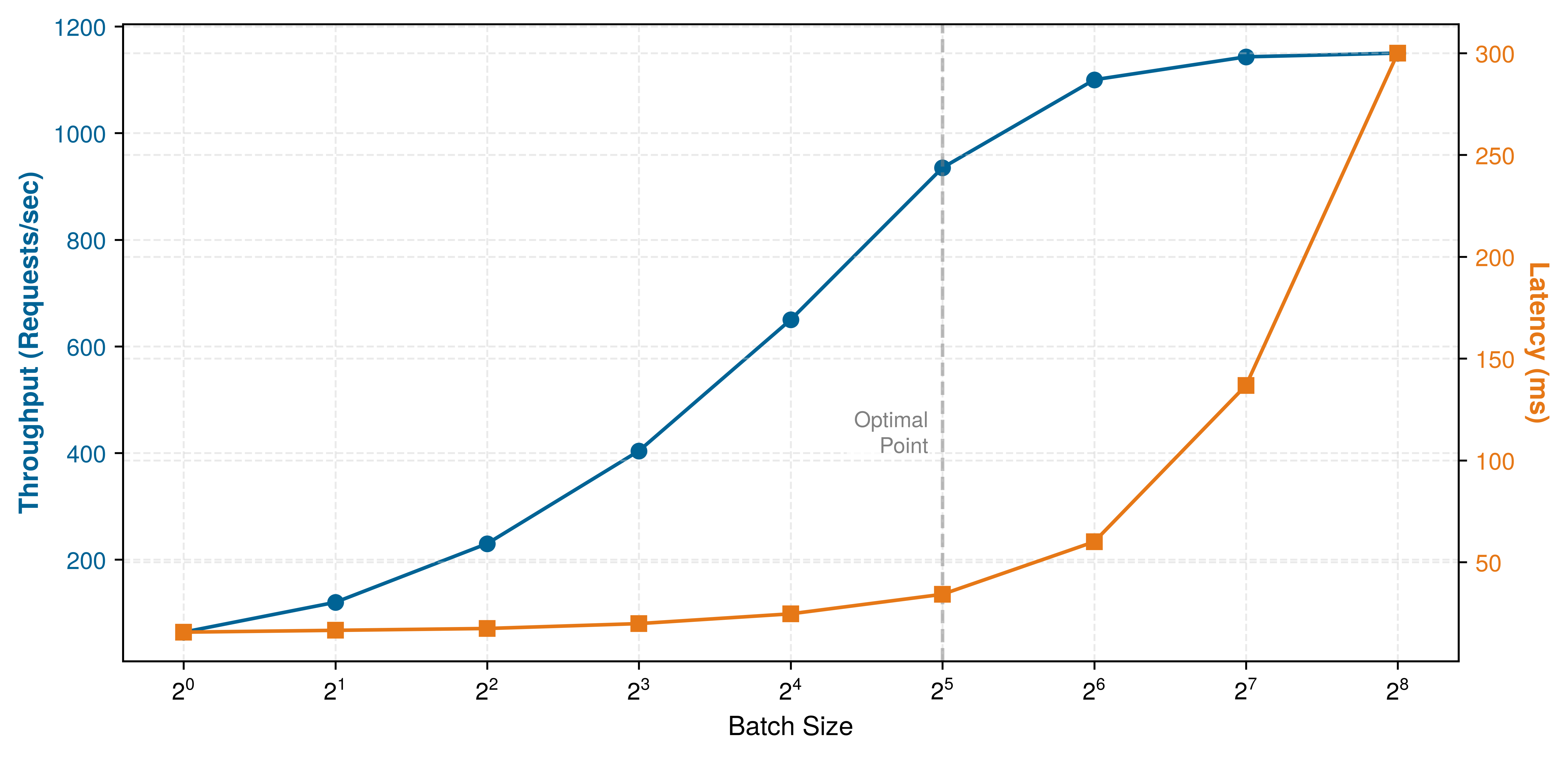
The “knee” in figure 6 marks the point where the blue throughput curve begins to plateau just as the orange latency curve starts its sharp upward spike. This is an illustrative knee rather than a universal optimum: the selected operating point depends on the latency SLO, arrival process, and cost objective. The numbers are representative rather than tied to a single benchmark.
Napkin Math 1.4: ResNet-50 batching efficiency
Table 9 illustrates the throughput-latency trade-off for a ResNet-50/V100 scenario across batch sizes one through thirty-two. The batch sizes, measured inference times, and GPU utilization are the scenario givens; the per-image compute and throughput columns are derived from them.
Table 9: ResNet-50 batching sweep: Illustrative per-image compute, throughput, and GPU utilization across batch sizes one through thirty-two on a V100. Throughput grows 6.4× from batch one to batch thirty-two as GPU utilization climbs from 15 percent to 95 percent, while pure inference time stretches from 5 ms to 25 ms.
Math: For the batch-8 row, we derive per-image compute by dividing the batch latency by batch size, 9.1 ms ÷ 8 images ≈ 1.1 ms per image, and throughput by dividing batch size by the same latency, 8 images ÷ 9.1 ms ≈ 879 img/s. We use the same two divisions for every derived row.
| Batch Size | Inference Time | Per-Image Compute | Throughput | GPU Util. |
|---|---|---|---|---|
| 1 | 5 ms | 5 ms | 200 img/s | 15% |
| 4 | 7.2 ms | 1.8 ms | 556 img/s | 42% |
| 8 | 9.1 ms | 1.1 ms | 879 img/s | 65% |
| 16 | 14 ms | 0.9 ms | 1,143 img/s | 85% |
| 32 | 25 ms | 0.8 ms | 1,280 img/s | 95% |
The times shown are pure inference time, excluding queue wait; section 1.7.6 analyzes how user-perceived latency includes batching-window wait.
Systems insight: Batch size thirty-two achieves 6.4× higher throughput than batch size 1. However, user-perceived latency includes both queue wait and inference time. With a 10 ms batching window and 25 ms inference, total latency reaches 35 ms vs. 5 ms at batch size 1.
The efficiency gains from batching come at a cost: requests must wait for the batch to form. This creates a direct tension between throughput optimization (larger batches) and latency minimization (immediate processing). The different batching strategies and their trade-offs govern how engineers tune this balance.
Static vs. dynamic batching
Static batching waits for a fixed batch size before processing, which is simple to implement but fragile under variable traffic: during low traffic, requests wait indefinitely for a full batch, and during high traffic, large batches increase per-request latency. Dynamic batching addresses this failure mode by collecting requests within a bounded time window and processing whatever has arrived when the window closes (Olston et al. 2017; NVIDIA 2024b). The window size becomes the tuning knob: shorter windows reduce latency but sacrifice throughput, longer windows improve throughput but increase latency, and latency-sensitive deployments tune both the time window and maximum batch size against arrival pattern, model shape, and SLO.
Dynamic batching latency-throughput trade-offs
Dynamic batching introduces a quantifiable tension between throughput optimization and latency constraints. Under overload, the mechanism is queue growth rather than slower inference, which enables systematic configuration decisions instead of trial-and-error tuning.
Systems Perspective 1.5: Why latency spikes under load
Recall from section 1.5.1 that Little’s Law \((Q_{\text{req}} = \lambda_{\text{arr}} T_{\text{lat}})\) relates long-run averages only while the queue is stable. As the arrival rate approaches the maximum service rate \(\mu\), the stable queue’s depth and latency grow rapidly. If \(\lambda_{\text{arr}}\) exceeds capacity for a sustained interval, no finite steady state exists: backlog accumulates until traffic falls, capacity grows, or work is rejected. This is why admission control can preserve latency during overload; scale-out or degraded service can also help when available.
Equation 7 decomposes the total user-perceived latency for a batched request into two components: \[L_{\text{lat}} = L_{\text{lat,wait}} + L_{\text{lat,compute}}(B) \tag{7}\] where \(L_{\text{lat,wait}}\) is the time spent waiting in the batching queue (corresponding to \(L_{\text{lat,queue}}\) in the overall latency budget) and \(L_{\text{lat,compute}}(B)\) is the inference time for batch size \(B\) (encompassing \(L_{\text{lat,infer}}\) plus portions of \(L_{\text{lat,pre}}\) and \(L_{\text{lat,post}}\)). The batching window \(T_{\text{window}}\) bounds wait time (\(L_{\text{lat,wait}} \leq T_{\text{window}}\)), while batch size affects compute time through GPU utilization characteristics.
Quantitative analysis of batching
For fixed calendar windows under stationary Poisson arrivals, request arrival times are uniform within each window. A request arriving at time \(t\) waits \(T_{\text{window}} - t\) for that window to close, so equation 8 gives an average wait of half the window: \[E[L_{\text{lat,wait}}] = \frac{T_{\text{window}}}{2} \tag{8}\]
This simple relationship has direct implications. A 20 ms batching window adds 10 ms average wait (up to 20 ms for the first arrival in a window; later arrivals wait less) regardless of batch size achieved. For a 50 ms mean latency SLO with 5 ms inference, the average wait consumes 20 percent of the latency budget before any computation begins; tail SLOs must budget the full window.
Batch size distribution
For fixed calendar windows, the number of requests collected during \(T_{\text{window}}\) follows a Poisson distribution with mean \(\lambda_{\text{arr}} T_{\text{window}}\). Equation 9 formalizes this relationship: \[\Pr(\text{batch size} = k) = \frac{(\lambda_{\text{arr}} T_{\text{window}})^k e^{-\lambda_{\text{arr}} T_{\text{window}}}}{k!} \tag{9}\]
Here \(k\) is a nonnegative integer count of arrivals in the window.
Table 10 quantifies this variability, showing how batch size fluctuates for different traffic levels with a fixed 10 ms window:
| Arrival Rate | Mean Batch | Std Dev | \(\Pr(\text{batch}=0)\) | \(\Pr(\text{batch} \ge 2 \times \text{mean})\) |
|---|---|---|---|---|
| 50 QPS | 0.5 | 0.7 | 61% | 39% |
| 200 QPS | 2 | 1.4 | 14% | 14% |
| 500 QPS | 5 | 2.2 | 0.7% | 3% |
| 1000 QPS | 10 | 3.2 | 0.005% | 0.3% |
Throughput maximization strategy
Throughput optimization requires separating per-request latency from saturated service capacity. A request waits for batch formation, then pays the service time of the formed batch. Under sustained load, however, batch formation can overlap with the previous batch’s execution, so capacity is governed by the ready-batch service time: \[\mu_{\text{eff}}(B) \approx \frac{B}{T_{\text{svc}}(B)}, \qquad \text{throughput} = \min(\lambda_{\text{arr}}, \mu_{\text{eff}}(B)) \tag{10}\]
In equation 10, \(\lambda_{\text{arr}}\) is the offered arrival rate and \(\mu_{\text{eff}}(B)\) is the saturated service capacity for batch size \(B\). The numerator increases linearly with batch size while service time often increases sub-linearly over a useful range because GPU parallelism is better used. The batching window still appears in request latency and in low-traffic regimes, where the expected batch size is limited by arrivals during the window, roughly \(\lambda_{\text{arr}} T_{\text{window}}\).
For ResNet-50 on a V100 GPU, service time approximately scales as \(T_{\text{svc}}(B) = 5 \text{ ms} + 0.6 B\) (5 ms fixed overhead plus 0.6 ms per image in the batch). This linear approximation captures the dominant trend; actual service times may deviate slightly due to memory hierarchy effects. With a \(T_{\text{window}} = 10 \text{ ms}\) batching window, table 11 extends the pure-inference sweep of table 9: latency includes the full-window wait bound, while saturated throughput uses service time alone:
| Batch Size | Service Time | Total Latency | Throughput | Efficiency |
|---|---|---|---|---|
| 1 | 5.6 ms | 15.6 ms | 179 img/s | Low |
| 4 | 7.4 ms | 17.4 ms | 541 img/s | Moderate |
| 8 | 9.8 ms | 19.8 ms | 816 img/s | Good |
| 16 | 14.6 ms | 24.6 ms | 1096 img/s | High |
| 32 | 24.2 ms | 34.2 ms | 1322 img/s | Maximum |
The throughput gains in table 11 trace directly back to the fixed-overhead term in the iron law established in Iron Law of Training Performance, where batching amortizes work across requests.
Example 1.7: The iron law of batching efficiency
Context: In serving, batching improves throughput by amortizing fixed per-batch scheduling and kernel-launch work; it can also amortize weight traffic across requests, while queue wait remains a separate latency cost. Holding the data-movement term outside this illustrative two-term comparison, equation 11 isolates compute and fixed overhead: \[ T = \frac{O}{R_{\text{peak}} \cdot \eta_{\text{hw}}} + L_{\text{lat}} \tag{11}\]
Analysis:
- Case 1 (batch 1): Overhead (5 ms) \(\gg\) Compute (0.6 ms). Efficiency ≈ 10 percent. The GPU is mostly waiting.
- Case 2 (batch 32): Overhead (5 ms) \(\ll\) Compute (19.2 ms). Efficiency ≈ 79 percent. The GPU is crunching numbers.
Systems insight: Increase batch size until fixed overhead becomes negligible (\(<\) 10 percent of total time) or the latency SLO blocks further waiting. Beyond this point, additional batching yields minimal throughput but imposes a linear queueing penalty.
These three results compose into one working model of dynamic batching: the window sets the average wait at half its length, Poisson arrivals make the realized batch size fluctuate around \(\lambda_{\text{arr}} T_{\text{window}}\), and the saturated service capacity \(\mu_{\text{eff}}(B)\) climbs with batch size until fixed overhead is amortized away. None of them yet enforces the latency SLO. The passes that follow add that missing constraint, working backward from a hard percentile budget to the largest batch the window may safely form.
Latency-constrained optimization
When latency SLOs provide the binding constraint, the optimization problem becomes finding the maximum batch size that meets the SLO. For a latency target \(L_{\text{lat,target}}\) and average wait time \(T_{\text{window}}/2\), equation 12 defines the maximum allowable batch size using a first-order average latency approximation: \[B_{\text{max}} = \max\left\{B : \frac{T_{\text{window}}}{2} + T_{\text{svc}}(B) \leq L_{\text{lat,target}}\right\} \tag{12}\]
In this illustrative ResNet-50 scenario with a 50 ms p95 latency SLO, comparing a conservative batching window against an aggressive one shows how the assumed configurations trade wait time, inference budget, and saturated capacity. Table 12 lays the two configurations side by side.
| Metric | Conservative (\(T_{\text{window}}\) = 5 ms) | Aggressive (\(T_{\text{window}}\) = 25 ms) |
|---|---|---|
| Average wait | 2.5 ms (max wait = 5 ms for the first request in a window) | 12.5 ms |
| Latency budget for inference | 47.5 ms (mean-latency planning; tail SLOs should budget the full window) | 37.5 ms |
| Batch size cap | 32 images | 48 |
| Assumed saturated capacity | ~1,140 img/s | ~1,280 img/s |
The aggressive configuration assumes 12.3 percent higher saturated capacity but increases average batching wait by 10 ms and the maximum window-wait contribution by 20 ms. The latter is not a p99-latency estimate.
SLO violation analysis
Batch size variability can cause SLO violations even when mean latency appears safe. A request in a fixed window sees itself plus the other arrivals, so \(B_{\text{req}}=1+\operatorname{Poisson}(\lambda_{\text{arr}}T_{\text{window}})\). Combining the full window with the request-seen p99 batch size gives the conservative envelope in equation 13: \[L_{\text{lat,envelope}} = T_{\text{window}} + T_{\text{svc}}(B_{\text{req,p99}}) \tag{13}\] For \(\lambda_{\text{arr}}\) = 500 QPS and \(T_{\text{window}}\) = 10 ms, the mean request-seen batch size is 6 and its p99 is 12. The mean latency is 13.6 ms; the conservative envelope is 22.2 ms.
The envelope is 1.63× the mean. It is not the request-latency p99 because full-window wait and p99 batch size need not occur for the same request.
Systems Perspective 1.6: The latency-throughput trade-off
A single “inference speed” number is undefined until the batch size is named, because batch size selects which regime, and which bottleneck, the system operates in.
- Batch-1 regime: Latency-oriented. Launch overhead or memory traffic often limits the request path. This regime governs real-time interaction such as typing helpers and robotics.
- Batch-N regime: Throughput-oriented. Larger batches amortize overhead and weight traffic and may shift the bottleneck toward compute. This regime governs offline processing and high-traffic services.
The two regimes optimize opposite quantities, so a model that is “fast” at batch 1 may be far from peak throughput, and vice versa. Any latency or throughput figure must therefore specify whether it was measured at single-stream latency (batch 1) or maximum throughput (batch N).
Adaptive batching windows
The same batch-size dependence drives how the serving system shapes its batches in the first place. Fixed batching windows waste latency budget during high traffic when large batches form quickly. Listing 2 demonstrates how adaptive strategies adjust the window based on queue depth.
In an illustrative scenario with traffic varying between 200–1000 QPS, a fixed 10 ms window produces 15 ms average latency at 650 img/s, while the adaptive heuristic produces 11 ms at 680 img/s. The interplay between window size and batch limits creates a space of possible configurations, each representing a different balance between throughput and latency.
def adaptive_batching_window(
    queue_depth, arrival_rate, slo_ms, service_ms, fixed_overhead_ms
):
    """Compute a heuristic batching window.

    Based on current system state.
    """
    target_batch_size = 16  # Deployment-tuned target batch

    # Fast path: batch ready, close immediately to minimize latency
    if queue_depth >= target_batch_size:
        return 0

    # Compute maximum allowable wait from the remaining p99 budget.
    max_wait_ms = max(0, slo_ms - service_ms - fixed_overhead_ms)

    # Estimate time to accumulate target batch at current arrival
    # rate.
    # arrival_rate is requests/second, so convert seconds to
    # milliseconds.
    if arrival_rate > 0:
        requests_needed = target_batch_size - queue_depth
        estimated_wait_ms = requests_needed / arrival_rate * 1000.0
        # Return minimum of estimated wait and SLO-constrained maximum
        return min(estimated_wait_ms, max_wait_ms)

    return max_wait_ms  # Low traffic: use remaining budget to accumulate batch
The nondominated batching configurations form a Pareto frontier where improving throughput requires accepting higher latency. Table 13 shows five illustrative configurations:
| Window (ms) | Max Batch | Avg Latency | p99 Latency | Throughput | Configuration |
|---|---|---|---|---|---|
| 2 | 16 | 8 ms | 18 ms | 890 img/s | Ultra-low latency |
| 5 | 32 | 10 ms | 22 ms | 1,140 img/s | Balanced |
| 10 | 32 | 15 ms | 35 ms | 1,240 img/s | Moderate latency |
| 20 | 64 | 23 ms | 52 ms | 1,310 img/s | Throughput-optimized |
| 50 | 128 | 38 ms | 98 ms | 1,350 img/s | Maximum throughput |
Practical configuration guidelines
The Pareto frontier in table 13 illustrates why configuration must work backward from the latency budget: past the knee, widening the window buys diminishing throughput for sharply rising tail latency. In the worked scenario, reserving 30 percent of the SLO for batching wait gives \(T_{\text{max}} = 0.3 \times L_{\text{lat,SLO}}\); another workload may allocate a different fraction after accounting for network, preprocessing, inference, and postprocessing. The traffic estimate should include peaks and burst duration rather than rely only on the mean. GPU memory supplies a separate ceiling on batch size through activations and runtime workspace. Finally, monitoring the realized batch-size and wait-time distributions reveals whether the assumed arrival model holds and whether a fixed or adaptive window is appropriate.
For an illustrative ResNet-50 serving system with a 50 ms SLO and 500 QPS traffic, the calculation turns the SLO and arrival-rate assumptions into two deployable knobs: the batching window and maximum batch size. Table 14 summarizes the resulting configuration and modeled operating point.
| Quantity | Value | Engineering role |
|---|---|---|
| Latency budget for batching | 15 ms | Portion of the SLO available for queueing delay. |
| Maximum window | 15 ms | Upper bound implied by the latency budget. |
| Expected request-seen batch | 7 | Average batch seen by an arriving request. |
| Request-seen p99 batch | 13 | Tail batch size under Poisson arrivals. |
| Assumed memory-limited batch | 32 | Scenario cap for accelerator memory. |
| Selected configuration | \(T_{\text{window}}\) = 12 ms, \(B_{\text{max}}\) = 32 | Practical knob setting for deployment. |
| Conservative tail envelope | 24.8 ms | Full window plus request-seen p99 batch service time. |
| Illustrative saturated capacity | 1,176.9 img/s | Estimate using the assumed 0.89 efficiency factor. |
| Served throughput | 500 img/s | Arrival-limited load handled by the configuration. |
Continuous batching
Autoregressive models like language models generate outputs token by token: each new token depends on all previously generated tokens, so generation is inherently sequential. The dynamic batching examined earlier in this section assumes fixed-length outputs. LLMs violate this assumption: if one sequence in a batch of eight finishes after ten tokens while others need 100 tokens, 90 percent of the compute for that sequence slot is wasted (Yu et al. 2022).
21 Continuous batching: Also called “iteration-level batching” (Yu et al. 2022) and, in NVIDIA TensorRT-LLM, “in-flight batching” (NVIDIA 2026f); the distinction is scheduling granularity. Traditional batching commits to a fixed batch for an entire generation sequence (potentially hundreds of iterations), while continuous batching reschedules at every token-generation step—analogous to preemptive OS process scheduling vs. run-to-completion. This finer granularity reduces the waste from variable-length sequences, where a batch slot occupied by a completed sequence sits idle until all other sequences finish.
Yu, Gyeong-In, Joo Seong Jeong, Geon-Woo Kim, Soojeong Kim, and Byung-Gon Chun. 2022. “Orca: A Distributed Serving System for Transformer-Based Generative Models.” 16th USENIX Symposium on Operating Systems Design and Implementation (OSDI 22), 521–38.
NVIDIA. 2026f. NVIDIA TensorRT-LLM.
Continuous batching21 (also called iteration-level batching) addresses this waste by allowing new requests to join a batch between generation steps and completed sequences to exit (Yu et al. 2022; Kwon et al. 2023). The system manages batch composition dynamically at each decoding iteration rather than forming static batches that persist for the entire generation process.
The mechanism works as follows: when a sequence generates its end-of-sequence token, its slot becomes immediately available. A waiting request can fill that slot for the next iteration rather than waiting for the entire batch to complete. Similarly, the system can add new requests to available slots without interrupting ongoing generation. This dynamic approach maintains high GPU utilization even when sequence lengths vary widely.
Systems implementing continuous batching, such as vLLM22 and TensorRT-LLM, improve throughput by keeping decode slots occupied as sequences enter and exit (Kwon et al. 2023; NVIDIA 2026f). Sarathi-Serve refines this scheduler with chunked prefill and stall-free batching to reduce interference between prompt processing and token decoding (Agrawal et al. 2024). The improvement comes from two sources: reducing wasted compute on completed sequences and reducing average wait time for new requests. For production language model serving where response lengths vary from single tokens to thousands, continuous batching has become a central technique for cost-effective deployment.
22 vLLM (virtual LLM): An open-source serving system that enables continuous batching via its PagedAttention algorithm (Kwon et al. 2023). Inspired by OS virtual memory, this technique reduces the severe KV-cache fragmentation and reservation waste that constrains static batching. By keeping KV-cache waste low, vLLM can serve larger effective batches on the same hardware.
Agrawal, Amey, Nitin Kedia, Ashish Panwar, Jayashree Mohan, Nipun Kwatra, Bhargav S. Gulavani, Alexey Tumanov, and Ramachandran Ramjee. 2024. “Taming Throughput-Latency Tradeoff in LLM Inference with Sarathi-Serve.” 18th USENIX Symposium on Operating Systems Design and Implementation (OSDI 24), 117–34.
Memory management adds complexity to continuous batching. As sequences enter and exit the batch, the key-value cache that stores attention context must be dynamically allocated and freed. Consider what happens when sequences of varying lengths share GPU memory: a 100-token sequence completes and releases its cache, but a new 150-token sequence cannot use that space because it needs a larger contiguous block. Over time, small unusable gaps accumulate between allocated regions, eventually preventing new sequences from starting even when total free memory appears sufficient. This memory fragmentation can waste 40 to 50 percent of available memory in naive implementations, severely limiting the concurrent batch size that determines throughput.
PagedAttention

PagedAttention recovers the KV-cache waste of contiguous allocation.
23 PagedAttention: The name directly references OS virtual memory paging, first implemented on the Atlas computer at Manchester (1962) to solve the same class of allocation problem—programs needed more memory than physically available, and contiguous allocation wasted space (Kilburn et al. 1962). Introduced at SOSP 2023, PagedAttention applies this six-decade-old abstraction to GPU KV-cache memory: before it, LLM serving systems wasted 60–80 percent of KV cache memory due to fragmentation and over-reservation. PagedAttention reduces waste to under 4 percent, enabling 2–4\(\times\) higher throughput on the same hardware (Kwon et al. 2023).
Kilburn, Tom, David B. G. Edwards, Michael J. Lanigan, and Frank H. Sumner. 1962. “One-Level Storage System.” IRE Transactions on Electronic Computers EC-11 (2): 223–35. https://doi.org/10.1109/TEC.1962.5219356.
Kwon, Woosuk, Zhuohan Li, Siyuan Zhuang, Ying Sheng, Lianmin Zheng, Cody Hao Yu, Joseph Gonzalez, Hao Zhang, and Ion Stoica. 2023. “Efficient Memory Management for Large Language Model Serving with PagedAttention.” Proceedings of the 29th Symposium on Operating Systems Principles, 611–26. https://doi.org/10.1145/3600006.3613165.
PagedAttention,23 introduced in vLLM, addresses this fragmentation problem by applying operating system virtual memory concepts to GPU memory (Kwon et al. 2023). In static contiguous allocation, reserving maximum sequence length memory up front causes internal waste, while freed regions may be too small or poorly placed to satisfy a new contiguous reservation. Instead of allocating one contiguous region per sequence, PagedAttention divides the KV cache into fixed-size blocks mapped through a block table. A sequence’s cache can therefore occupy noncontiguous physical blocks. When a sequence completes, its blocks return to a free pool for reuse. The vLLM paper reports KV-cache waste below 4 percent and higher throughput than the compared systems; exact gains depend on workload and implementation.
The batching and memory techniques covered here establish the foundation for LLM serving, but several advanced topics warrant additional study.
Systems Perspective 1.7: LLM serving: Beyond the fundamentals
Language model serving introduces challenges beyond the batching and memory principles established here. The key-value cache that stores attention context scales with sequence length and batch size, often exceeding the model weights themselves in memory consumption. Techniques like speculative decoding use small draft models to propose multiple tokens that the target model verifies in parallel; evaluated T5-XXL workloads achieved roughly 2–3\(\times\) speedups (Leviathan et al. 2023), but gains vary. Weight-only quantization (such as INT4 weights with FP16 activations) is especially relevant for memory-bandwidth-bound LLM inference (Lin et al. 2024).
These LLM-specific optimizations build directly on the foundations this chapter establishes: queuing theory governs request scheduling, batching trade-offs determine throughput-latency curves, and precision selection follows the same accuracy-efficiency principles. The same serving fundamentals remain applicable, while LLM serving adds domain-specific techniques atop them. Advanced treatments provide detailed coverage of KV cache optimization, including techniques for multi-tenant serving, where one fleet shares capacity across users, and distributed inference, where one request may be split across machines.
Continuous batching is widely used for high-throughput LLM serving, yet not all deployment scenarios benefit from batching. The techniques examined so far, from dynamic batching windows to PagedAttention, target shared server workloads. They introduce scheduler and memory-management complexity that may not be justified in every deployment. The practical question is when batching hurts rather than helps.
Some scenarios favor single-request processing. Under an ultra-low p99 target, even a short batching timeout may consume too much of the budget. Highly variable request sizes create padding overhead because shorter inputs may be padded to match the longest input in a batch. Memory can also bind when weights already consume most accelerator memory, since batched activations and cache state can trigger out-of-memory errors.
Session affinity constraints
When requests from the same user or session should route to the same replica, batching becomes constrained. Session affinity, also called sticky sessions, matters for three main reasons.
The most impactful case is KV-cache reuse in conversational AI, where the key-value cache from previous turns can materially speed up multi-turn conversations. Routing a follow-up request to a different replica forfeits this cached context, forcing the system to recompute or reload prefix state for long conversations.
A second driver is user-specific models: some systems serve personalized models or adapters per user, and routing requests to the replica that has already loaded that user’s adapter avoids repeated loading overhead. Similarly, stateful preprocessing that maintains tokenizer caches or session-specific normalization requires rebuilding state when requests route to a different replica.
The tension with batching is clear since strict affinity constrains which requests can be batched together, potentially reducing batch sizes and GPU utilization. Production systems often implement soft affinity where requests prefer their assigned replica but can overflow to others when that replica is overloaded. This preserves most affinity benefits while maintaining load balance.
Traffic patterns and batching strategy
The batching strategy depends critically on how requests arrive. Different deployment contexts exhibit different arrival patterns, and the MLPerf inference benchmark supplies four standardized scenarios that approximate several common cases, as MLPerf execution scenarios explains in detail.
Server traffic (Poisson arrivals)
The MLPerf Server scenario models cloud/API-like inference traffic with Poisson arrivals (Reddi et al. 2019).24 Under that model, counts in disjoint intervals are independent and the average arrival rate is constant. Equation 14 expresses the expected count in a fixed calendar window with rate \(\lambda_{\text{arr}}\) and width \(T_{\text{window}}\): \[E[\text{batch size}] = \lambda_{\text{arr}} \cdot T_{\text{window}} \tag{14}\]
Reddi, Vijay Janapa, Christine Cheng, David Kanter, Peter Mattson, Guenther Schmuelling, Carole-Jean Wu, Brian Anderson, et al. 2019. “MLPerf Inference Benchmark.” 2020 ACM/IEEE 47th Annual International Symposium on Computer Architecture (ISCA), 446–59. https://doi.org/10.1109/isca45697.2020.00045.
24 Poisson process: Named after French mathematician Simeon Denis Poisson (1781–1840), this stochastic model describes events occurring continuously and independently at a constant average rate. In fixed calendar windows, variance equals the mean, so with \(\lambda_{\text{arr}}=200\) req/s and a 10 ms window, the expected count is two and roughly 14 percent of windows are empty, though an efficient scheduler launches no GPU work for them. A request-triggered timer instead begins with one request and counts only additional arrivals during the window.
For fixed calendar windows, variance equals the mean, so batch sizes fluctuate significantly at moderate traffic. With \(\lambda_{\text{arr}} = 200\) requests/second and \(T_{\text{window}} = 10\) ms, the expected count is two, but roughly 14 percent of windows have zero requests (and launch no GPU work) while others may have four or more.
A useful heuristic for the batching window balances waiting cost against throughput benefit. Equation 15 expresses one such rule: \[T_{\text{window}} \approx \min\left(L_{\text{lat,SLO}} - T_{\text{svc}}, \sqrt{\frac{T_{\text{svc}}}{\lambda_{\text{arr}}}}\right) \tag{15}\] where \(L_{\text{lat,SLO}}\) is the latency SLO, \(T_{\text{svc}}\) is the service time (in seconds), and \(\lambda_{\text{arr}}\) is the arrival rate (in requests per second), making the second term dimensionally consistent in seconds. The square-root form is a local cost-model heuristic: it balances a fixed per-batch benefit against a waiting cost that grows with the arrival interval. It is not a closed-form optimum for ML serving specifically; production systems calibrate the window empirically against observed traffic. A counterintuitive result emerges from equation 15: as traffic increases, the optimal window decreases while achieved batch sizes still grow. Table 15 demonstrates this phenomenon across four traffic levels.

As QPS rises, the batching window shrinks while batch size grows.
| Arrival Rate | Optimal Window | Avg Batch Size | Approx. Latency |
|---|---|---|---|
| 100 QPS | 15.8 ms | 1.6 | 40.8 ms |
| 500 QPS | 7.1 ms | 3.5 | 32.1 ms |
| 1,000 QPS | 5 ms | 5 | 30 ms |
| 5,000 QPS | 2.24 ms | 11.2 | 27.2 ms |
Single-user traffic (sequential arrivals)
Streaming traffic correlates arrivals through sensor synchronization, making batch size and deadline externally fixed. At the opposite end of the spectrum, some interactive mobile and embedded applications have little opportunity to batch independent requests. The optimization target shifts from a synchronization budget under a hard frame deadline to per-request latency and energy consumption under a thermal power envelope.
Many interactive mobile and embedded applications process one request stream at a time; the MLPerf SingleStream scenario captures this sequential-serving shape. For the ResNet-50 phone scenario used here, the dominant costs shift from batch formation to per-request latency and energy.
Mobile serving constraints
Cloud services often emphasize fleet cost and latency; mobile serving adds three closely coupled constraints. The first is an energy budget that throughput alone does not capture, because each inference consumes battery. In the modeled pipeline, 2.98 mJ at 22 FPS draws about 66 mW for the inference path alone, before camera, display, ISP, and OS overhead add to that total in a full photo app. Thermal throttling can compound this limit when sustained system power reaches a device-specific thermal boundary. Memory constraints close the set because the model shares RAM with the application and operating system. Reload time depends on device storage, runtime, and model state; quantization and memory-mapped loading (section 1.6.3) can reduce footprint and startup work but do not eliminate those dependencies.
Example 1.9: ResNet-50: Mobile serving
Table 17 decomposes per-phase latency and energy for a single-user mobile vision inference:
| Phase | Duration | Energy | Notes |
|---|---|---|---|
| Camera buffer read | 8 ms | 0.08 mJ | System API |
| JPEG decode (CPU) | 15 ms | 1.5 mJ | Single-threaded |
| Resize + Normalize | 5 ms | 0.4 mJ | CPU preprocessing |
| NPU inference | 12 ms | 0.8 mJ | 82% utilization |
| Postprocess + UI | 5 ms | 0.2 mJ | Result rendering |
| Total | 45 ms | 2.98 mJ | 22 FPS sustained |
The mobile serving node is governed by four metrics:
- Energy per inference: 2.98 mJ enables ~12.1M inferences per 10 Wh battery (typical smartphone)
- Modeled inference power: 2.98 mJ / 45 ms = 66 mW, excluding the rest of the device and therefore not a guarantee of indefinite operation
- NPU vs. CPU trade-off: CPU fallback replaces the 12 ms, 0.8 mJ NPU inference stage with a 45 ms, 4.2 mJ CPU stage; the full pipeline would rise from 45 ms and 2.98 mJ to about 78 ms and 6.4 mJ before additional system overhead.
- Memory footprint: 150 MB peak (model + activations), competing with app memory
Systems insight: In this illustrative pipeline, the mobile NPU reaches 82 percent utilization at batch size one while the data-center example reaches 15 percent. The contrast is workload- and hardware-specific, but it shows why a mobile accelerator designed for single-stream execution can operate efficiently without the batches used to amortize a large server GPU.
These constraints make mobile serving optimization qualitatively different from cloud optimization. The goal is not maximum throughput but sustainable performance, maintaining acceptable latency without thermal throttling or excessive battery drain. Strict latency budgets make synchronized multi-camera frame processing challenging (table 16). In a 30 FPS autonomous driving pipeline (33 ms total budget), frame capture and arrival jitter consume 15 ms before inference can begin. Batching 6 camera streams into a single GPU invocation completes in 10 ms (at \(T=25\) ms), leaving 7 ms for postprocessing, planning, and safety checks. If frame jitter pushes the start past 15 ms, the pipeline misses its deadline.
Traffic pattern summary
Traffic-adaptive batching adjusts the batching window as queue depth and request rate change. Table 18 relates the four MLPerf scenarios to representative deployment contexts and common batching strategies.
These scenarios are benchmark abstractions rather than deployment prescriptions. The operative batching policy must still follow the service’s current concurrency, deadline, and power constraints.
| Scenario | Context | Strategy | Focus |
|---|---|---|---|
| Server | Cloud APIs, web services | Dynamic batching with timeout | Window tuning, utilization-latency curve |
| MultiStream | Autonomous driving, video analytics | Synchronized sensor fusion | Jitter handling, deadline guarantees |
| SingleStream | Mobile apps, embedded devices | No batching (\(B = 1\)) | Preprocessing, power efficiency |
| Offline | Batch processing, data pipelines | Maximum batch size | Throughput, hardware utilization |
The MLPerf Server scenario captures cloud API traffic, MultiStream captures synchronized sensor workloads, and Offline inference captures batch processing where throughput dominates latency.
The batching strategies examined so far share a critical assumption: each request produces a single, fixed-size output—one classification label, one bounding box, one embedding vector. This assumption governs the queuing math, the Pareto frontier analysis, and the traffic-adaptive window tuning. The fastest-growing category of serving workloads, however, violates this assumption entirely. Large language models generate outputs token by token, with each token depending on every previous one. A single request may produce hundreds or thousands of tokens over seconds of elapsed time, yet must feel responsive from the first token onward. This fundamental shift from fixed-output to variable-length, streaming-output serving builds directly on the continuous batching and KV-cache paging already established for autoregressive generation. What it adds are phase-split metrics for prefill and decode, decoding strategies that trade output quality against per-token cost, and memory tactics such as prefix reuse and offloading that exploit shared context.
Checkpoint 1.3: Batching and traffic patterns
Batching is the primary lever for serving economics, but the optimal strategy depends on context.
Self-Check: Question
Why does increasing the batch size during deep learning inference dramatically improve hardware throughput on modern GPUs, and at what point does throughput plateau on the Roofline model?
- Batching converts all floating-point operations into integer bitshifts, bypassing GPU ALUs entirely.
- Batching reduces the total parameter count of the neural network by sharing weights across batch samples.
- Batching eliminates PCIe bus data transfer overhead by generating synthetic input tensors on the device.
- Batching increases arithmetic intensity (FLOPs per byte of memory accessed) by reusing loaded weight matrices across multiple input samples, shifting the workload from memory-bandwidth-bound to compute-bound until compute saturates.
Contrast traditional request-level dynamic batching with iteration-level continuous batching (as introduced in Orca and vLLM) for Large Language Model (LLM) serving. Why is request-level batching severely inefficient for autoregressive generation?
True or False: PagedAttention resolves the primary memory waste in LLM KV-caching by allocating key and value states in non-contiguous, fixed-size physical memory blocks managed via a virtual page table, eliminating both internal fragmentation from over-allocation and external memory fragmentation.
An autonomous vehicle perceives its environment using 6 surround cameras that capture frames simultaneously at 30 Hz. Because all camera frames arrive at the perception server simultaneously in synchronized bursts, this represents a ____ arrival process that enables zero-wait co-batching across camera streams.
A cloud serving system with an end-to-end latency budget of 50 ms configures a dynamic batcher with
max_batch_size = 32andmax_batch_delay_ms = 20. Under low traffic (10 QPS), individual requests arrive 100 ms apart. What is the operational impact on latency and batch efficiency?- Every request waits the full 20 ms timeout in the queue and executes as a batch of size 1, incurring the maximum queueing delay penalty with zero throughput amortization gain.
- Requests are automatically dropped because the queue fails to reach the maximum batch size of 32 within 50 ms.
- The server achieves peak GPU utilization because small batches execute with sub-microsecond latency.
- The dynamic batcher disables timeouts and waits indefinitely until 32 requests accumulate, preserving throughput at the cost of infinite latency.
LLM Serving
Large language models make three properties far more prominent than in fixed-output serving: autoregressive generation25 (each token depends on all previous tokens, making output inherently sequential), variable-length output (response length is unknown at request time, complicating fixed-batch assumptions), and stateful memory (the key-value cache grows with each generated token, creating dynamic memory pressure). Together, these properties create a qualitatively different serving challenge. The p50, p95, and p99 metrics used for classification serving still matter, but they apply to different phases of the request—the initial prompt processing and the subsequent token generation. The same principles of queuing theory, batching trade-offs, and latency budgets remain applicable; LLM serving adds domain-specific techniques atop them.
25 Autoregressive: From Greek auto- (self) and Latin regressus (a going back)—the output “regresses” on itself; George Udny Yule introduced autoregressive models in 1927 for analyzing sunspot cycles. In language modeling, each output token conditions on all previously generated tokens, creating a serial dependency that prevents the parallelism exploited during training. Decode is often weight-bandwidth-bound at small batches; larger batches amortize the weight stream and can shift the bottleneck toward compute or KV-cache traffic (Pope et al. 2023).
Pope, Reiner, Sholto Douglas, Aakanksha Chowdhery, Jacob Devlin, James Bradbury, Jonathan Heek, Kefan Xiao, Shivani Agrawal, and Jeff Dean. 2023. “Efficiently Scaling Transformer Inference.” Proceedings of Machine Learning and Systems (MLSys) 5: 606–24.
Performance metrics: TTFT and TPOT
TTFT and TPOT live in different bottleneck regimes.
Generative models produce a stream of tokens rather than a single output tensor. This streaming nature requires dedicated LLM performance metrics that reflect the transition from prefill (processing the prompt and populating its KV cache) to decode (generating output). Two key measures are time to first token (TTFT) and time per output token (TPOT), which capture responsiveness and average generation pace. Per-gap Inter-Token Latency (ITL) measures the distribution of pauses between individual streamed tokens; TPOT instead averages the post-first-token interval across an output.
Definition 1.6: LLM performance metrics
LLM performance metrics separate initial responsiveness from the cadence of streaming autoregressive generation.
- Significance: They decompose user-perceived latency into time to first token (TTFT) (whose prefill work is often compute-bound) and time per output token (TPOT) (whose decode work is often bandwidth-bound at small batches).
- Distinction: Unlike fixed-output metrics (for example, end-to-end latency), LLM metrics measure the fluidity of generation, acknowledging that the user experience depends on the rhythm of token arrival.
- Common pitfall: A frequent misconception is that a “fast model” has a low TTFT. In reality, a model can have a fast TTFT but a sluggish TPOT (if the memory wall \((\text{BW})\) is the bottleneck), leading to a frustrating user experience where the answer starts quickly but “stutters” thereafter.
These metrics capture distinct aspects of the user experience, so interactive services often set separate targets for TTFT, TPOT or ITL, and aggregate throughput.
Systems Perspective 1.8: LLM serving latency targets
Interactive LLM services usually need separate SLOs for responsiveness, generation fluidity, and fleet throughput. The following values are illustrative targets rather than universal requirements:
- TTFT: \(<\) 500 ms (for a 1000-token prompt)
- TPOT: \(<\) 50 ms (equivalent to ~20 tokens/s, faster than human reading speed)
- Throughput: \(>\) 1000 tokens/s aggregate across active serving replicas
A single “latency” number therefore hides the prefill/decode split. TTFT is the blank-screen budget, TPOT is the reading-flow budget, and aggregate service throughput, measured as tokens/s summed across active serving replicas, determines whether those targets hold under shared load.
Decoding strategies
Meeting these TPOT targets depends on more than memory bandwidth alone: the algorithm used to select each token also affects per-token latency and output quality. Generative models require decoding strategies that trade off quality, diversity, and latency. The choice of decoding strategy dramatically affects both output quality and computational cost.
The simplest approach, greedy decoding, selects the highest-probability token at each step at the cost of one model pass per token. It is fast but can produce repetitive outputs because it cannot recover from early choices. Beam search maintains multiple candidate sequences and selects a high-scoring complete sequence, increasing decoder work and state relative to greedy decoding. Sampling with temperature, top-\(k\), and top-\(p\) (also called nucleus sampling) injects controlled randomness for diversity (Holtzman et al. 2020). The serving cost of any strategy depends on its implementation and on the output-length distribution that continuous batching must absorb.
Holtzman, Ari, Jan Buys, Li Du, Maxwell Forbes, and Yejin Choi. 2020. “The Curious Case of Neural Text Degeneration.” Proceedings of the 8th International Conference on Learning Representations (ICLR 2020).
Interactive LLM services commonly return tokens as they are produced rather than waiting for complete generation. This streaming response transforms the user experience: a two-second total generation feels responsive when tokens stream continuously, but feels broken when users stare at a blank screen for two seconds. Streaming requires infrastructure support for incremental responses and client-side rendering. The latency profile shifts accordingly: TTFT determines when output starts appearing (responsiveness), while TPOT determines the perceived generation speed (fluidity). Once generation is streamed token by token, the serving unit changes from one fixed-output prediction to a stateful sequence whose memory footprint grows on every step.
Memory and KV cache
Generative inference requires managing the KV Cache26, a stateful memory structure that grows with sequence length. Prefill creates cache entries for prompt tokens, and each decoded token adds another entry. Across concurrent variable-length sequences, this dynamic state can dominate available accelerator memory and create allocation waste if it is not managed explicitly.
26 KV cache (key-value cache): To avoid redundant work, the system caches the Key and Value vectors from previous tokens, which remain valid throughout generation; this design choice is the direct cause of the dynamic memory growth described; the cache’s size grows linearly with every generated token, making memory management a primary constraint. For the 70-billion-parameter-class grouped-query-attention sizing example in this calculation, the FP16 KV cache is about 0.33 MB per token per sequence; grouped-query attention (GQA), used in Llama-family models such as Llama 3, shares key/value heads across multiple query heads, reducing the cache relative to full multi-head attention (Dubey et al. 2024). A batch of 32 requests at an 8,000-token context therefore requires roughly 80 GB just for KV cache, several times larger still without grouped-query or multi-query attention.
Dubey, Abhimanyu, Abhinav Jauhri, Abhinav Pandey, Abhishek Kadian, et al. 2024. The Llama 3 Herd of Models. arXiv preprint arXiv:2407.21783.
Prefix caching and memory offloading
The continuous batching and PagedAttention techniques covered in section 1.7.4 address request scheduling and cache paging; the remaining memory pressure can be further mitigated through architectural strategies that exploit request patterns. Prefix caching stores the KV states of common instruction prefixes (such as a 2,000-token system prompt or a shared retrieval-augmented generation (RAG) context), allowing independent requests to reuse the prefill result for an identical prefix. For \(N\) requests sharing a prefix of \(S_{\text{prefix}}\) tokens, the avoided prefill work is roughly \((N-1)S_{\text{prefix}}\) token steps, subject to cache hits, eviction, and implementation overhead. For multi-turn conversations, the same principle lets a subsequent turn process only the new suffix after reusing compatible prior state.
Napkin Math 1.5: The energy cost of a chat
Problem: How much energy does an H100-backed chat service spend per generated token and for a response with 500 tokens?
As LLMs scale, joules per token becomes a first-class operational metric alongside latency. Assuming the H100 draws its 700 W thermal design power (TDP), this scenario estimate follows from throughput and power (Choquette 2023):
- Throughput: 114 concurrent requests \(\times\) 8 tokens/s per request ≈ 912 tokens/s.
- Power: 700 W (GPU) + 300 W (Host/Overhead) = 1000 W.
- Energy per token: 1000 W / 912 tokens/s ≈ 1.0965 J/token
Systems insight: Under these assumptions, a response of 500 tokens consumes ≈ 548.2 J.
- For comparison, charging a smartphone consumes ≈ 40000 J.
- Boiling a cup of water consumes ≈ 100000 J.
The primary way to reduce J/token is to increase hardware utilization and eliminate redundant compute. If the GPU sits at 10 percent utilization due to poor batching, it still draws ~300 W and the host adds 300 W, causing energy per token to rise to 6.6 J/token (approximately 6× the baseline). Architectural optimizations like prefix caching also skip the energy-intensive prefill phase for shared context, directly reducing the energy footprint of retrieval-augmented generation (RAG) and chat applications. The serving lesson is that efficiency is not only a latency or cost metric; it also determines how much energy each useful token consumes.
27 Speculative decoding: A small “draft” model generates \(k\) candidate tokens autoregressively; the large target model then verifies the proposed block in parallel (Leviathan et al. 2023). When the draft model’s proposals are accepted at rate \(\alpha\), effective throughput can scale with the number of accepted tokens per verification step. This breaks the serial autoregressive bottleneck at the runtime layer, not the architecture layer.
Leviathan, Yaniv, Matan Kalman, and Yossi Matias. 2023. “Fast Inference from Transformers via Speculative Decoding.” International Conference on Machine Learning (ICML), 19274–86.
When the aggregate KV cache exceeds GPU VRAM, systems can employ KV cache offloading. This strategy spills inactive or low-priority context windows to host CPU RAM or NVMe SSD, freeing VRAM for active generation. The reload cost is bounded below by bytes moved divided by PCIe or NVMe bandwidth, before software overhead and queueing are added. Offloading therefore prevents OOM failures and enables larger context windows, but it also creates affinity, invalidation, and hot-decode latency risks that must be budgeted explicitly. Advanced techniques including speculative decoding27 and distributed parallelism, where one request is split across multiple devices or machines, are covered in specialized treatments of large-scale systems.
Checkpoint 1.4: LLM serving fundamentals
LLM serving introduces constraints absent from traditional model serving.
The chat-energy calculation makes utilization part of the LLM serving budget: the cost of each generated token depends on how requests share the machine. Unlike fixed-output inference, LLM energy grows with response length. Each decode step streams weights once for the active batch, so batching amortizes that traffic across sequences. Carbon accounting additionally requires an emissions factor and a defined boundary.
Energy efficiency depends on the same batching, memory, and prefix-cache mechanisms that govern LLM latency, so the useful summary is a constraint checklist rather than a single scalar metric.
Self-Check: Question
In Large Language Model (LLM) serving, how do the computational and hardware characteristics of the Prefill phase (Time to First Token, TTFT) fundamentally differ from the Decode phase (Time Per Output Token, TPOT)?
- Prefill processes tokens autoregressively one by one and is memory-bandwidth bound, whereas Decode processes all output tokens simultaneously and is compute-bound.
- Prefill processes all prompt tokens concurrently in parallel matrix multiplications and is compute-bound, whereas Decode generates one token per step autoregressively and is memory-bandwidth bound due to repeated weight fetching.
- Prefill operates exclusively on host CPU DRAM, whereas Decode runs on GPU Tensor Cores.
- Prefill latency scales quadratically with batch size, whereas Decode latency is strictly independent of sequence length and KV-cache size.
Calculate the total memory footprint (in bytes) required to store the KV cache for a batch of \(B = 16\) requests, each with an active context length of \(S = 2\text{,}048\) tokens, for a model with \(L = 32\) transformer layers, \(H_{\text{kv}} = 8\) key-value attention heads (Grouped-Query Attention), head dimension \(D_{\text{head}} = 128\), stored in FP16 precision (\(P = 2\text{ bytes}\)).
Order the step-by-step execution cycle of Speculative Decoding for accelerating LLM inference:
- Target model runs a single parallel forward pass over the prompt plus all \(K\) draft candidate tokens to compute ground-truth verification logits
- Draft model (a lightweight autoregressive model) generates \(K\) candidate tokens sequentially in fast memory-bandwidth-efficient steps
- Engine appends the accepted tokens (plus one newly corrected token) to the KV cache and advances the generation context
- Verification logic evaluates draft tokens against target logits (using greedy matching or modified rejection sampling) to accept the first \(M\) matching tokens (\(M \le K\))
True or False: Speculative decoding alters the output token probability distribution of the target LLM, trading mathematical output fidelity and generation accuracy for higher decoding speed.
In a multi-turn conversational AI system with extensive system prompts (e.g., 2,000 tokens of instructions and few-shot examples shared across thousands of user sessions), what serving optimization eliminates redundant prefill compute across requests?
- Linear Attention Approximation, which drops system prompt tokens entirely from the attention window.
- Static Graph Compilation, which hardcodes user inputs directly into the weight tensors.
- Prefix Caching (e.g., RadixAttention), which stores the KV-cache states of common prompt prefixes in memory and reuses them across queries matching the prefix.
- Speculative Quantization, which quantizes prompt tokens into 1-bit binary representations during the decode phase.
Inference Runtime Selection
The batching strategies and LLM-specific techniques determine how requests are grouped and processed. These strategies assume an underlying execution engine that actually runs the model computations. The token generation dynamics introduced in section 1.8 and the latency budgets established in section 1.4.1 are achievable only if the runtime maps operations efficiently to hardware. The inference runtime, the software layer that orchestrates tensor operations and manages hardware resources, can materially change performance for the same model. Runtime work therefore has two phases: selection chooses the execution engine, and configuration tunes that engine for the target model, hardware, input shapes, and latency distribution.
Runtime ecosystem and configuration
Selection should start with the binding constraint rather than the framework used during training. When deployment speed and framework compatibility dominate, PyTorch and TensorFlow models can often serve through their native runtimes without a separate interchange export. This preserves support for more of the training framework’s operators and control flow, although custom operations, device support, and production packaging can still limit deployability. Framework runtimes also carry generality that a target-specific inference engine may trade for tighter optimization.
torch.export and TensorFlow SavedModel provide serialized graphs for ahead-of-time transformation and graph optimization while maintaining framework compatibility. TorchScript remains a legacy format for existing deployments.
General-purpose optimization
When portability across hardware is the binding constraint, ONNX Runtime28 provides a hardware-agnostic optimization layer (Microsoft 2024). Models export to ONNX format, then ONNX Runtime applies graph optimizations and selects execution providers for the target hardware. This enables single-format deployment across CPUs, GPUs, and specialized accelerators.
28 ONNX Runtime: Microsoft’s inference engine acts as a hardware abstraction layer: the same ONNX model can run on CPUs, NVIDIA GPUs, AMD GPUs, or custom accelerators through pluggable execution providers. ONNX Runtime applies graph optimizations such as constant folding, redundant-node elimination, and operator fusion. Performance relative to a tuned target-specific engine such as TensorRT depends on the workload, execution provider, and hardware.
Microsoft. 2024. ONNX Runtime: Cross-Platform Inference and Training Machine-Learning Accelerator. GitHub.
Portability still requires inspecting operator placement. An unsupported operation may fall back to another execution provider, introducing host-device transfers and synchronization that preserve correctness while erasing the expected speedup. Profiling must therefore verify provider assignment and operator coverage, not only whether the exported graph runs.
Specialized inference engines
When latency or hardware cost binds more tightly than portability, TensorRT29 (NVIDIA GPUs), OpenVINO30 (Intel hardware), and similar engines optimize specifically for their target hardware (NVIDIA 2024a; Intel Corporation 2026; Chen et al. 2018). They apply aggressive target-specific optimizations that framework-native runtimes may not apply uniformly across hardware.
29 TensorRT: It abandons the portability of general-purpose frameworks by requiring a build phase that optimizes the model for a target GPU architecture (for example, an H100) (NVIDIA 2024a). This hardware lock-in allows aggressive optimizations like layer fusion and precision selection that portable runtimes may not apply uniformly across targets. The resulting nonportable engine can materially reduce latency and therefore the number of GPUs required to meet a throughput target.
NVIDIA. 2024a. NVIDIA TensorRT: Programmable Inference Accelerator.
30 OpenVINO (open visual inference and neural network optimization): An Intel-oriented inference toolkit that converts, optimizes, and runs models across Intel CPU, GPU, and NPU targets (Intel Corporation 2026). This direct hardware targeting is an “aggressive” optimization because it abandons some portability that framework-native runtimes must guarantee, allowing it to exploit target-specific kernels and precision choices. The resulting performance gain is workload- and hardware-dependent, but it can make dedicated CPU or edge serving economically viable for smaller and latency-sensitive models.
Intel Corporation. 2026. OpenVINO Documentation.
Chen, Tianqi, Thierry Moreau, Ziheng Jiang, Lianmin Zheng, Eddie Q. Yan, Haichen Shen, Meghan Cowan, et al. 2018. “TVM: An Automated End-to-End Optimizing Compiler for Deep Learning.” Proceedings of the 13th USENIX Symposium on Operating Systems Design and Implementation (OSDI ’18), 578–94.
31 Layer fusion: Analogous to loop fusion in compiler optimization, where adjacent loops over the same array are combined to reduce memory traffic. Kernel fusion applies the same principle to GPU operations: sequential kernels that write and re-read intermediate tensors from HBM are merged into a single kernel that can keep data in registers.
Layer fusion31 combines multiple sequential operations into a single GPU kernel. Consider convolution → batch normalization → rectified linear unit (ReLU) activation. Without fusion, this requires three kernel launches and two intermediate write/read round-trips. Fusion combines all three into one kernel that reads inputs once, computes the combined result in registers, and writes final outputs once.
Kernel auto-tuning selects the fastest algorithm for each operation on the specific GPU. A single convolution can be implemented using dozens of algorithms such as direct, FFT-based, Winograd, and various tiling strategies, each optimal for different input sizes and GPU architectures. Auto-tuning benchmarks each candidate and caches the winner, trading compilation time for runtime performance.
These optimizations can produce substantial speedups over an untuned framework-native baseline, but they require explicit export or compilation and may not support every operation or dynamic shape. The illustrative runtime comparison that follows quantifies one such optimization spectrum.
Example 1.10: ResNet-50: Runtime comparison
Table 19 gives an illustrative batch-one ResNet-50/V100 runtime scenario:
Table 19: Illustrative inference runtime comparison: Assumed latency and derived speedup for batch-one ResNet-50 across PyTorch eager, TorchScript, ONNX Runtime, and TensorRT on a V100.
| Runtime | Latency | Speedup | Notes |
|---|---|---|---|
| PyTorch (eager) | 8.5 ms | 1× | Baseline, no optimization |
| TorchScript | 6.2 ms | 1.4× | JIT compilation |
| ONNX Runtime | 5.1 ms | 1.7× | Cross-platform |
| TensorRT FP32 | 2.8 ms | 3× | NVIDIA-specific |
| TensorRT FP16 | 1.4 ms | 6.1× | Tensor Core acceleration |
| TensorRT INT8 | 0.9 ms | 9.4× | Requires calibration |
Systems insight: In this illustrative comparison, TensorRT INT8 provides 9.4× speedup and requires quantization calibration data and NVIDIA-specific deployment.
The optimization-compatibility trade-off is inherent. More aggressive optimization yields better performance yet increases deployment complexity and may introduce numerical differences from training. The choice depends on latency requirements, deployment constraints, and available engineering resources.
After the runtime is chosen, configuration applies the same constraint-first logic. Thread pool sizing controls parallelism for CPU inference: too few threads leave cores idle, while too many cause contention. Memory allocation strategies (preallocated buffers vs. dynamic allocation) trade startup cost against flexibility. Execution provider selection prioritizes which hardware backends handle each operation, and graph optimization level trades compilation time for runtime performance. These settings are not a separate checklist after selection; they are how the selected runtime is made honest under production traffic. Production deployments therefore measure configuration impact on latency distributions rather than relying on defaults.
Precision selection for serving
In an illustrative scenario, a team deploying ResNet-50 on V100 GPUs assumes that switching from FP32 to INT8 on the non-Tensor-Core integer path triples throughput and costs less than 0.4 percentage points of accuracy. This example illustrates the direct connection between numerical precision and infrastructure economics. Precision selection connects to the quantization techniques covered in Quantization and Precision. Numerical Representations compares the numerical formats (FP32, FP16, BF16, FP8, INT8) and their precision-range trade-offs, and Integer quantization details the mechanics of symmetric and asymmetric integer quantization. Serving adds runtime concerns such as calibration data availability, layer sensitivity under production inputs, and dynamic precision selection.
Precision-throughput relationship
For memory-bandwidth-bound operations, reducing precision can raise throughput by reducing data movement. Equation 16 gives the bandwidth-only upper bound from precision reduction: \[ \frac{\text{Throughput}_{\text{INT8}}}{\text{Throughput}_{\text{FP32}}} = \frac{32}{8} = 4\times \text{ (theoretical maximum)} \tag{16}\]
Actual speedup depends on the hardware, operator mix, calibration, and kernel alignment, and therefore falls below the bandwidth-only bound whenever another constraint intervenes. Low-precision kernels are most efficient when matrix dimensions fit the target accelerator’s preferred tile shapes. Modern cuBLAS and cuDNN can still use Tensor Cores for many other dimensions, though sometimes less efficiently or with internal padding. Tensor Cores provides the detailed Tensor Core architecture that explains these alignment constraints. The precision trade-offs for a standard vision model illustrate how these theoretical limits manifest in practice.
Example 1.11: ResNet-50: Precision trade-offs on V100
Table 20 gives illustrative latency, memory, and accuracy assumptions across FP32, FP16, and two INT8 paths for ResNet-50, together with Tensor Core utilization where supported:
Table 20: Illustrative precision trade-offs on V100: Assumed latency, memory footprint, and accuracy for ResNet-50 in FP32, FP16, and INT8 (PTQ and QAT), plus Tensor Core utilization where supported.
| Precision | Latency | Memory | Accuracy | Tensor Core Util. | Calibration |
|---|---|---|---|---|---|
| FP32 | 2.8 ms | 98 MB | 76.13% | 0% | None |
| FP16 | 1.4 ms | 49 MB | 76.13% | 85% | None |
| INT8 (PTQ) | 0.9 ms | 25 MB | 75.80% | N/A | 1,000 samples |
| INT8 (QAT) | 0.9 ms | 25 MB | 76.05% | N/A | Additional training |
Systems insight: In this illustrative scenario, INT8 provides 3.1× speedup and loses 0.33 percentage points of accuracy with PTQ. QAT recovers most of that loss but requires retraining.
Precision selection constraints
Precision selection is constrained by layer sensitivity, calibration data, and runtime policy. Not all layers tolerate reduced precision equally. For a scalar uniform \(b\)-bit quantizer over the calibrated range \([\alpha,\beta]\), the step and within-range rounding-error bound in equation 17 are \[\Delta = \frac{\beta-\alpha}{2^b-1}, \qquad |\epsilon_{\text{quant}}| \leq \frac{\Delta}{2} \tag{17}\] for values that are not clipped. Values outside the calibrated range are clipped and may incur greater error. Layer-level output or task error also depends on activation distributions and downstream sensitivity, so it must be measured rather than inferred from a universal norm law. This explains observed patterns where first convolutional and final classification layers are often retained at FP16, while middle layers shown by calibration and task-level evaluation to tolerate reduced precision use INT8.
Post-training quantization adds a data constraint. The calibration dataset determines the scale factors used for INT8 conversion, so it must represent actual serving traffic rather than merely reuse convenient training or validation data. A calibration-serving mismatch can degrade task accuracy, a failure mode revisited in section 1.12.
Advanced serving systems turn precision into a runtime policy. If the system is ahead of its latency SLO, it can use higher precision for better accuracy. For low-confidence INT8 results, it can recompute at FP16. Different customer tiers may receive different precision levels. This pattern enables adaptive quality-latency trade-offs while maximizing throughput during normal operation.
The precision decision has direct infrastructure consequences: under the illustrative 3\(\times\) throughput assumption, a workload requiring 30 GPUs at FP32 needs 10 at INT8 if all other constraints remain unchanged. The connection between model-level optimization and infrastructure economics is why precision selection cannot be treated as purely a model concern.
Self-Check: Question
An ML systems team is deploying a transformer-based ranking model on NVIDIA data center GPUs. They consider running the raw PyTorch model in eager Python mode versus compiling the model into an optimized NVIDIA TensorRT engine. Which optimization does TensorRT perform that PyTorch eager mode cannot achieve?
- TensorRT automatically converts the supervised classification task into an unsupervised reinforcement learning policy.
- TensorRT trains additional adapter layers during live request serving to adapt to data drift.
- TensorRT eliminates all GPU memory usage by running inferences exclusively in the CPU instruction cache.
- TensorRT performs aggressive vertical and horizontal operator fusion (e.g., combining Conv/MatMul, BiasAdd, and Activation into a single kernel), eliminates redundant memory round-trips, and selects hardware-tuned cuDNN/Tensor Core kernels.
Why does quantizing a model’s weights and activations from FP16 to INT8 for GPU serving often yield a \(2\times\) or greater throughput improvement, and what role does Post-Training Quantization (PTQ) calibration play in preserving accuracy?
True or False: In deep neural network quantization, certain layers (such as the initial embedding/convolution layer, final classification projection, and attention softmax score calculations) exhibit high sensitivity to precision loss, and preserving them in FP16/FP32 while quantizing remaining bulk layers to INT8/INT4 (mixed-precision serving) frequently prevents model accuracy collapse.
When deploying models to edge devices with Apple Silicon (such as iPhones and iPads), developers export models to the ____ framework to take full advantage of the dedicated Apple Neural Engine (ANE) hardware accelerator.
When calibrating an INT8 quantized model using Post-Training Quantization (PTQ), what is the primary danger of using a synthetic or unrepresentative calibration dataset (e.g., ImageNet validation images for a medical endoscopy model)?
- The activation dynamic ranges and outlier distributions in production will not match the calibration dataset, leading to severe clipping of real-world features or coarse quantization binning that degrades serving accuracy.
- The model compiler will fail to generate valid GPU assembly code and reject the weights.
- The server’s physical power consumption will double due to misaligned integer registers.
- The dynamic batcher will permanently lock its batch size to 1.
Node-Level Optimization
Runtime selection and precision tuning operate at the model level: they determine what computation runs and at what numerical format. Between the model and the silicon, however, lies another optimization layer encompassing the mechanics of graph compilation to kernels, byte movement from disk to memory, and CPU-GPU coordination. Node-level work closes the gap between a model benchmark and the complete request path, but its gain depends on which boundary the measured trace identifies as binding.
Consider an image classifier whose model benchmark promises millisecond inference but whose production trace shows a slower request path. Node-level optimization identifies which boundary is wasting time on that machine. The trace usually points to one of four recurring diagnostic boundaries:
- Graph-to-kernel boundary: The computation graph has to become a small number of efficient kernels rather than a long sequence of launch overheads.
- CPU execution boundary: CPU-side work has to exploit vector units, locality, and runtime libraries rather than scalar Python.
- Load boundary: Model bytes have to move from disk into memory fast enough that cold starts do not dominate scale-up events.
- Host-accelerator boundary: The host has to keep the accelerator scheduled without gaps caused by preprocessing, transfers, or synchronization.
These are not independent tricks. They are places where a measured trace can explain why a request path is slower than the model benchmark promised.
Runtime graph compilation
Inference engines like TensorRT were introduced in section 1.9. They can outperform an untuned eager baseline because serving often gives the compiler more stable operators and a bounded set of input-shape profiles. When those properties hold, the compiler can spend deployment-time work to remove runtime work; services with highly dynamic control flow or shapes retain fewer of these opportunities.
The first gain is operator fusion, the same kernel-merging optimization section 1.9.1.2 applied to TensorRT. What the static serving graph adds is when the fusion happens: because operators and shapes are fixed before any request arrives, the compiler can discover and commit the fused kernels ahead of time rather than rediscovering them at runtime, so no request pays for the analysis.
The same static graph also enables constant folding. If a subexpression depends only on fixed weights or constants, such as x * (sqrt(2) / 2), the compiler replaces it with the precomputed multiplication x * 0.707.... This removes work from every request without changing the model’s mathematical output.
Memory planning applies the same idea to allocation rather than arithmetic. Since the tensor lifetimes are known, the runtime can precalculate memory offsets and reuse buffers instead of allocating reactively during the request. This eliminates operations while creating a predictable serving path with fewer allocator stalls and less memory fragmentation.
Systems Perspective 1.9: Compilation timing trade-off
Just-in-time compilation waits until the graph is first executed and can specialize to the shapes it observes. That specialization is useful for variable traffic, but it moves compiler work into the serving path and creates a cold-request latency spike.
Ahead-of-time compilation performs the compiler work before deployment. It gives the service a fixed graph and avoids startup compilation latency, at the cost of defining all dynamic shapes explicitly or compiling multiple profiles.
Compilation cost can be paid at two points. JIT pays it in the serving path and risks a first-request latency spike, while ahead-of-time compilation pays it before deployment and requires tighter control over input shapes.
These optimizations lead to a deployment choice. Just-in-time compilation adapts to the shapes observed at runtime, but the first request pays the compilation penalty. Ahead-of-time compilation removes that startup spike by shipping an optimized artifact, but the deployment must explicitly cover every shape profile the service will accept.
CPU inference optimization
CPU inference faces its own optimization landscape, where vectorization, locality, graph optimization, and quantization work together. CPUs remain practical for many inference workloads, especially small models, latency-insensitive jobs, and deployments that cannot keep an accelerator busy. Modern CPUs32 (Intel Xeon, AMD EPYC) contain vector and matrix units such as AVX-512 and AMX, but scalar Python does not exercise them directly. Specialized runtimes such as OpenVINO map neural network operators to optimized kernels that use these instructions (Intel Corporation 2026).
32 SIMD (single instruction, multiple data): From Michael Flynn’s 1966 taxonomy of computer architectures, SIMD enables one instruction to operate on multiple data elements simultaneously. Intel’s AVX-512 can process sixteen FP32 values in a 512-bit vector, while AMX adds matrix tile operations. The attainable fraction of peak depends on data type, matrix shape, memory behavior, and implementation, but optimized kernels can be dramatically more efficient than scalar code.
33 NUMA (non-uniform memory access): Accessing memory local to a CPU socket is faster than accessing memory attached to a different socket; pinning an inference thread to a core is insufficient if its required memory is allocated remotely, forcing traffic across the slower inter-socket link. This failure to co-locate threads and data imposes a workload-dependent latency overhead. The exact penalty depends on socket topology, memory placement, and access pattern, but it can be substantial for memory-bound ML workloads because model weights can exceed L3 cache capacity, causing cross-socket fetches on cache misses.
The next CPU boundary is locality. On multi-socket servers,33 accessing data on another CPU socket incurs non-uniform memory access (NUMA) latency. An inference server must therefore be NUMA-aware: threads should be pinned to specific cores, and the model weights and input buffers those threads touch should be allocated on the same socket. ML model weights—hundreds of megabytes for a mid-sized network and gigabytes for a large language model—can exceed a CPU’s L3 cache, so the NUMA penalty can be persistent rather than occasional. Inference may repeatedly stream substantial portions of the weight tensor from main RAM, forcing fetches across the slower inter-socket link when locality is not preserved.
For sufficiently small models at batch size one, a CPU can outperform a GPU when accelerator launch, synchronization, and transfer overhead exceed the useful compute time. Model size alone does not determine the crossover; operator mix, resident data, runtime, CPU vectorization, and the latency target must be measured on the candidate hardware.
Model serialization and fast loading
Autoscaling systems are operational control loops that add or remove serving replicas based on load. In those systems, the time to spin up a new node is critical. A major component of “Cold Start” (section 1.6.2) is simply reading the model weights from disk into memory. The choice of serialization format determines how quickly this loading can occur.
PyTorch checkpoints loaded through torch.load() use a zip-based serialization container with pickle-encoded metadata; safe loading modes restrict which objects may be reconstructed, but the format still performs framework-specific deserialization. A tensor-oriented format34 can reduce object reconstruction and extra host copies. Memory mapping, introduced in section 1.6.3, further allows tensor bytes to be exposed from the file on demand when the serialized layout is compatible with the CPU tensor view.
34 Safetensors: The name emphasizes safety: unlike unrestricted pickle deserialization, the format does not encode executable Python objects (Hugging Face 2026). It stores tensors as contiguous raw bytes with a small header and supports memory-mapped loading. In the local benchmark example, that path is 10× faster than the compared PyTorch checkpoint path; the result is workload- and storage-specific and does not include transfer to a discrete accelerator.
Hugging Face. 2026. Safetensors Documentation.
Building on this principle, Safetensors is a tensor format designed for safe, efficient loading. It stores tensor metadata in a small header and tensor values as contiguous bytes, enabling memory-mapped CPU access without reconstructing arbitrary Python objects. Moving those tensors to a discrete accelerator still requires device transfer unless the platform provides a compatible shared-memory path.
Example 1.12: Loading speed: Safetensors vs. Pickle
Scenario: A serverless inference replica loads a 5 GB model checkpoint during cold-start scaling events.
Diagnosis: PyTorch torch.load() (Pickle) requires CPU object reconstruction, taking 15 s to initialize. Safetensors memory-mapping bypasses CPU parsing, loading weights in 1.5 s (10× faster).
Systems lesson: Tensor-oriented, memory-mapped formats can reduce CPU reconstruction and eager-copy overhead during cold start. Storage throughput, page faults, runtime initialization, and accelerator transfer still remain in the scale-out budget.
Profiling the serving node
Optimization without measurement is guesswork. The system efficiency metric defined in equation 2 provides the target: maximizing the fraction of wall-clock time the accelerator spends on useful computation. Timeline profiling tools like PyTorch Profiler or NVIDIA Nsight Systems (nsys) make that target visible by showing the exact sequence of events on the CPU and GPU.
A useful trace reading is bottleneck-first. Empty spaces in the GPU bar mean idle hardware, usually because the GPU is waiting for CPU preprocessing or disk I/O. Thousands of tiny GPU slivers indicate excessive kernel launches and point toward operator fusion or graph compilation. MemcpyHtoD blocks expose host-to-device movement; the diagnostic question is whether those transfers overlap with computation or block it. The timeline therefore converts a vague complaint about slow serving into a concrete boundary in the request path.
Example 1.13: The profiling loop
Scenario: An inference serving node exhibits high p99 tail latency despite low average GPU compute utilization.
Diagnosis: Timeline profiling (Nsight Systems/PyTorch Profiler) reveals large idle gaps between tiny GPU kernels caused by CPU host-side preprocessing bottlenecks and kernel launch overhead.
Systems lesson: Serving node optimization requires empirical timeline profiling. Iteratively identifying trace bottlenecks (kernel launch overhead, host-device copy stalls) guides targeted optimizations like operator fusion and pinned memory.
Table 21 is a decision aid rather than a checklist: choose the technique whose target metric matches the measured bottleneck, not the row with the largest displayed gain.
| Technique | Target Metric | Illustrative Gain | Implement. Cost | Best For |
|---|---|---|---|---|
| Operator Fusion | Latency & Throughput | 2–5\(\times\) | Medium (Compiler) | Memory-bound layers |
| INT8 Quantization | Throughput | 3–4\(\times\) | High (Calibration) | Inference-heavy nodes |
| Graph Compilation | Latency | 1.5–3\(\times\) | Low (One-line) | Static graph models |
| Zero-Copy Loading | Startup Time | 10–50\(\times\) | Low (File format) | Autoscaling/Cold Start |
| CPU Pinning | Tail Latency (p99) | 20–50% reduction | Low (Config) | Latency-critical apps |
This hierarchy of impact guides where to invest engineering effort. A layered checkpoint keeps that prioritization tied to the serving stack, from request transport down to fused kernels.
Checkpoint 1.5: The optimization hierarchy
Optimizing inference follows the request path from the outside in.
The stack has four levels.
Self-Check: Question
Why does loading model weights from modern
safetensorsformat provide substantially faster container startup times than legacy PyTorch.ptor.bin(Pythonpickle) files?safetensorsfiles compress weights using gzip, reducing disk storage by \(10\times\).safetensorsfiles store pure, uncompressed raw byte arrays aligned to page boundaries, allowing zero-copy memory mapping (mmap) directly into host memory without running Python object deserialization or arbitrary code execution.safetensorsfiles compile PyTorch code directly into binary x86 machine instructions on disk.safetensorsfiles automatically quantize FP32 weights into 4-bit integers during read operations.
In a CPU-based model serving deployment, how do vector extensions like Intel Advanced Matrix Extensions (AMX) or Vector Neural Network Instructions (VNNI) accelerate inference throughput compared to standard scalar x86 execution?
Order the iterative steps of an end-to-end performance profiling workflow for diagnosing an inference serving bottleneck:
- Inspect timeline traces (e.g., via Nsight Systems or PyTorch Profiler) to identify gaps, CUDA stream stalls, CPU-GPU synchronization, and memory bandwidth utilization
- Implement targeted optimization (e.g., kernel fusion, precision reduction, or CPU pipelining) on the identified bottleneck stage
- Establish a reproducible baseline by driving realistic synthetic load with a benchmarking tool (e.g., Triton Perf Analyzer) and measuring latency percentiles (p50, p99)
- Re-benchmark under identical load to verify latency reduction and ensure model prediction accuracy remains intact
- Identify the binding bottleneck category (Compute-bound, Memory-bandwidth-bound, or Host/Pipeline-bound)
True or False: In Ahead-of-Time (AOT) graph compilation, operator fusion is restricted to combining adjacent layers of the exact same mathematical type (e.g., fusing two consecutive Conv2D operations).
When profiling a GPU inference server under high load, an engineer observes that the GPU utilization metric reported by
nvidia-smiis 95%, but Nsight Systems timeline traces reveal that the GPU is actually spending 40% of its time stalled on host CPU memory copies. What accounts for this discrepancy?nvidia-smimeasures fan speed and ambient temperature rather than compute kernel activity.- The GPU memory clock is automatically halved during Nsight Systems tracing.
- The CPU is running at 100% duty cycle, which forces
nvidia-smito report false GPU metrics. nvidia-smireports the percentage of time a GPU kernel or context was active on the device, treating memory-stalled or synchronous PCIe transfer states as ‘active’ utilization rather than measuring true compute ALU duty cycle.
Economics and Planning
Batching, precision tuning, operator fusion, and graph compilation can reduce latency, increase capacity, or lower the cost of a completed inference. Production deployment, however, requires answering a fleet-level question: how many machines, of what type, at what total cost. A team that achieves 1,200 images/second on a V100 still needs to know whether 8 V100s at $3/hour each or 24 T4s at $0.53/hour each yields lower cost for its 5,000 QPS target while meeting the same SLO. Serving infrastructure cost grows with sustained request volume (Zhang et al. 2019), while training cost follows its own dataset, model, and optimization budget. The public API price compression shown in figure 2 illustrates this pressure: as per-token prices fall, infrastructure efficiency becomes a primary lever for economic viability.
Zhang, Chengliang, Minchen Yu, Wei Wang, and Feng Yan. 2019. “MArk: Exploiting Cloud Services for Cost-Effective, SLO-Aware Machine Learning Inference Serving.” 2019 USENIX Annual Technical Conference (USENIX ATC 19), 1049–62.
Cost per inference
Cost per inference divides the allocated serving cost over the number of completed inferences that satisfy the service objective. The numerator can include provisioned CPU or accelerator time, memory capacity, data transfer, storage, and orchestration. At high utilization, useful throughput spreads that provisioned cost across many requests. At low utilization, paid capacity sits idle, so the same hourly bill is divided among fewer successful inferences. Applying the framework to ResNet-50 shows how hourly price and sustained valid throughput combine into a unit cost.
GPU vs. CPU economics
In the worked AWS cost analysis in section 1.11.1, GPU instances cost more per hour but deliver much higher parallel throughput. The crossover point depends on model characteristics and latency requirements.
CPU inference makes economic sense for small models with few parameters and simple operations, when latency requirements are relaxed (hundreds of milliseconds acceptable), when request volume is low or highly variable (making GPU reservation wasteful), or when the model’s operations do not parallelize well. GPU inference is attractive when models are large with parallel-friendly operations, latency requirements are strict (tens of milliseconds), request volume is high and consistent enough to sustain utilization, and batching can amortize the per-inference overhead of GPU kernel launches.
Beyond steady-state costs, startup time affects scaling economics. Instance launch, image pull, driver initialization, model loading, compilation, and warmup can make accelerator replicas slower to become ready than CPU replicas, although exact times depend on the platform and deployment artifact. If traffic rises faster than useful capacity can come online, latency SLOs can fail despite sufficient eventual capacity.
When accelerator replicas have a long readiness delay, predictive scaling or a warm pool may be more reliable than purely reactive scaling. For a model that runs acceptably on both device types, a hybrid design can use always-on accelerator capacity for baseline load and CPU overflow for spikes, trading a different unit cost and latency profile for faster reserve capacity. This GPU+CPU hybrid is one instance of the broader patterns cataloged in Hybrid Architectures; whether it works depends on model compatibility and identical output semantics across runtimes.
Example 1.14: ResNet-50: Cost analysis
Table 22 gives an illustrative AWS-like scenario for hourly cost, throughput, and per-million-image cost when serving ResNet-50:
Table 22: Illustrative ResNet-50 cloud inference cost comparison: Assumed hourly cost and saturated throughput, with derived cost per one million images for CPU, T4, and V100 instances.
| Instance Type | Cost/Hour | Throughput | Cost per 1M Images |
|---|---|---|---|
| c5.xlarge (CPU) | $0.17 | 50 img/s | $0.94 |
| g4dn.xlarge (T4 GPU) | $0.53 | 400 img/s | $0.37 |
| p3.2xlarge (V100 GPU) | $3.06 | 1,200 img/s | $0.71 |
Systems insight: The T4 GPU instance has the lowest unit cost under these assumptions. The V100 does not beat the T4 on unit cost at the stated full-utilization rates. Cloud pricing varies by region and changes over time; consult current pricing for production planning.
Capacity planning
The GPU vs. CPU decision establishes the cost per inference, but determining how much infrastructure to provision requires combining cost analysis with the queuing theory foundations from section 1.5. Capacity planning translates three inputs into infrastructure specifications: traffic patterns (peak request rate, daily/weekly cycles, growth projections), latency SLOs (p50, p95, p99 targets), and model characteristics (inference time distribution at various batch sizes) (Harchol-Balter 2013).
Harchol-Balter, Mor. 2013. Performance Modeling and Design of Computer Systems: Queueing Theory in Action. Cambridge University Press. https://doi.org/10.1017/cbo9781139226424.
The worked example in section 1.5 demonstrates the complete workflow: starting from a 50 ms p99 SLO and 5,000 QPS target, deriving the conservative M/M/1 safe utilization threshold of 54 percent from equation 6, and determining GPU count with headroom of 62 V100s. This scenario provisions peak load plus 30 percent headroom; production margins depend on the workload and policy. Autoscaling can reduce costs during low-traffic periods while meeting latency objectives during peaks; ML Operations develops the operational policy layer around these serving calculations. Throughput numbers are meaningful only when coupled with latency guarantees. As the valid-QPS accounting in section 1.5 established, capacity must be sized for requests that actually meet the SLO, not for raw request volume.
Production case study: Serving 8-billion-parameter Llama 3
Beyond resident weights, KV-cache memory is often one of the largest capacity costs in large-language-model serving, and figure 7 shows why. Plotted at 70-billion-parameter scale to amplify the effect, the cache grows linearly with context length and batch size until long contexts exhaust the memory left after loading weights and runtime workspace. The 8-billion-parameter Llama 3 profile analyzed in the rest of this section obeys the same physics with more headroom, making it a workload an engineer can fit on one GPU and reason about end to end.
Workload profile
The following fixed workload assumptions define the reference case used throughout the latency, memory, and economics calculations in this section; together, they bound the analyses that follow.
- Model: 8-billion-parameter Llama 3 (quantized to 4-bit using activation-aware weight quantization (AWQ); see Quantization and Precision for quantization techniques) (Dubey et al. 2024; Lin et al. 2024).
- Hardware: 1\(\times\) NVIDIA H100 SXM5 GPU (80 GB HBM3, 3.35 TB/s bandwidth) (Choquette 2023).
- Request characteristics: 1,000-token input prompt (Prefill), 256-token generated response (Decode).
- Target SLOs: TTFT \(<\) 200 ms, TPOT \(<\) 20 ms.
Lin, Ji, Jiaming Tang, Haotian Tang, Shang Yang, Wei-Ming Chen, Wei-Chen Wang, Guangxuan Xiao, Xingyu Dang, Chuang Gan, and Song Han. 2024. “AWQ: Activation-Aware Weight Quantization for on-Device LLM Compression and Acceleration.” Proceedings of Machine Learning and Systems 6: 87–100.
Choquette, Jack. 2023. “NVIDIA Hopper H100 GPU: Scaling Performance.” IEEE Micro 43 (3): 9–17. https://doi.org/10.1109/mm.2023.3256796.
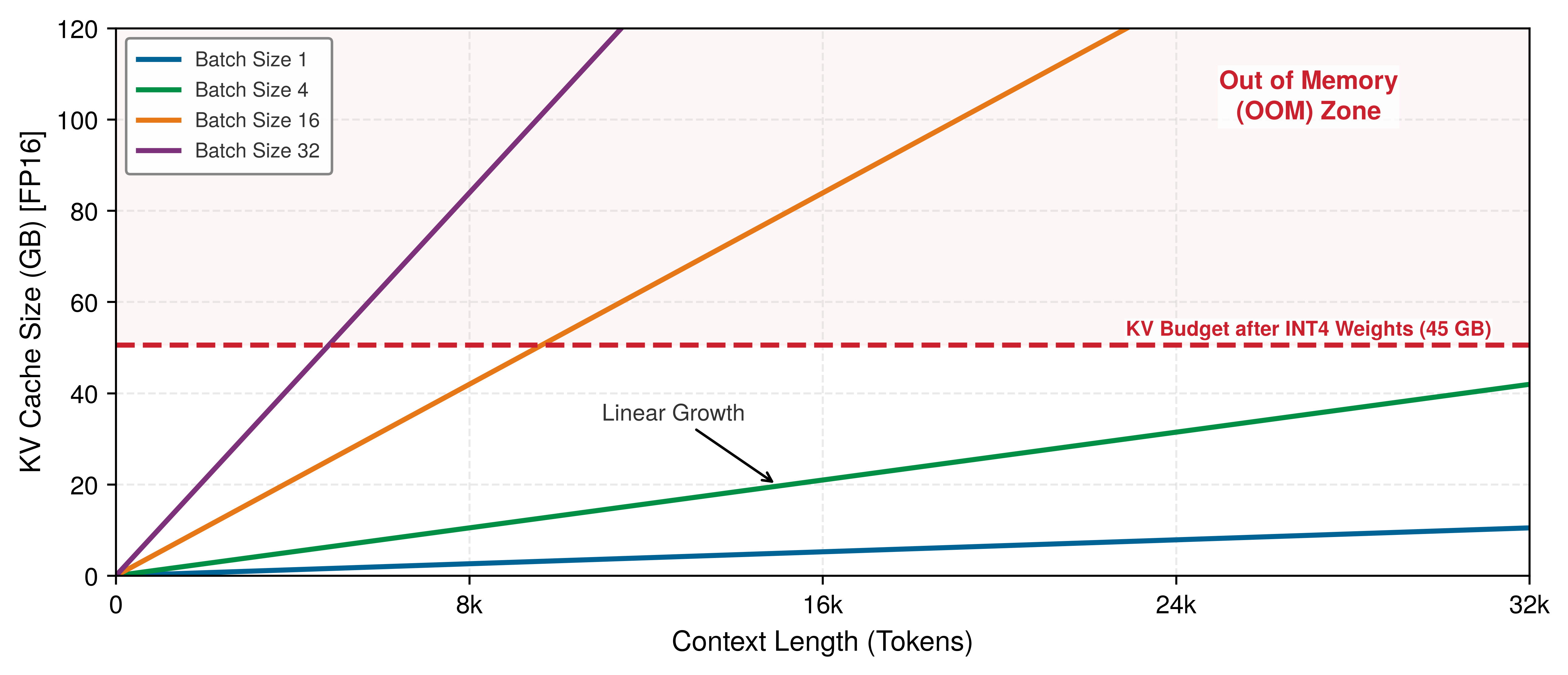
Longer contexts therefore require smaller concurrent batches or more memory, reducing throughput efficiency.
These assumptions make the case study narrow enough to calculate while preserving the two serving constraints that matter most: the prefill budget for time to first token and the decode budget for each generated token.
Latency deconstruction
The end-to-end request latency is governed by the two-phase execution model of autoregressive transformers, applying the TTFT and TPOT metrics defined in section 1.8.1. Prefill determines whether the user sees a prompt response quickly; decode determines whether the generated stream keeps moving after it starts.
Systems Perspective 1.10: The physics of token generation
Recall the energy-movement invariant quantified in Energy Cost of Moving vs. Computing on a 32-Bit Value: moving a bit is 100–1,000\(\times\) more expensive than computing on it. In the decode phase, this law determines the physical “cost per word.”
Physics: For batch-one decode with INT4 weights, the weight-dominated arithmetic intensity is approximately \(2\) FLOPs per parameter divided by \(0.5\) byte per parameter, or \(4\) FLOPs/byte. This is far below the H100 ridge point, so the modeled step is memory-bandwidth bound. Larger decode batches reuse the weight stream across sequences and raise arithmetic intensity (Pope et al. 2023). The batch-one bandwidth floor is captured in equation 18: \[ T_{\text{token}} \approx \frac{D_{\text{vol}}}{\text{BW}_{\text{memory}}} \tag{18}\]
Implication: Every token generation pays an energy cost to move model weights from HBM into compute registers. On an A100 80 GB (2.04 TB/s HBM2e), the same model has a theoretical weight-streaming floor of approximately 1.97 ms per token. When decode remains bandwidth-bound, adding more compute cores yields little latency improvement; faster memory (Physics), smaller models (Algorithm), or better batching and cache management change the bound.
Prefill phase (time to first token)
The model processes the 1,000-token prompt in parallel. Under the solver’s stated 40 percent compute-efficiency assumption, the model-side TTFT estimate is 41.9 ms, comfortably within the 200 ms SLO and leaving the remaining budget for network ingress, tokenization, and queueing.
Decode phase (time per output token)
The model generates 256 tokens sequentially. At batch one, this phase is memory-bandwidth bound: each step streams the 4 GB weight tensor from VRAM. A batched step amortizes that stream across its active sequences.
To obtain the theoretical floor, we divide the 4 GB weight tensor by the 3.35 TB/s bandwidth: \(T_{\text{token}} \approx\) 1.2 ms. Adding the solver’s per-layer dispatch tax gives a modeled TPOT of 1.57 ms. Generating all 256 tokens therefore takes 256 tokens \(\times\) 1.57 ms = 0.40 s.
Memory and throughput
With 4-bit weights occupying 4 GB, the remaining ~81.9 GB is available for the KV cache and runtime workspace. Each token requires approximately 0.131 MB of FP16 KV cache in the 8-billion-parameter Llama 3 configuration, since grouped-query attention reduces KV-head storage relative to full multi-head attention; AWQ is weight-only and does not make that cache INT4. Dividing the 72 GB reserve by that per-token cost yields capacity for ≈ 0.6 million tokens, so at 1,256 tokens the GPU can hold a concurrent batch size of ~469 requests.
Unit economics
Consider a representative H100 SXM5 rental cost of approximately $3/hour. Taking the minimum of isolated prefill capacity and KV-residency capacity gives an optimistic throughput ceiling of 45.2 million tokens/hour and a lower-bound unit cost of $0.066/million tokens. This calculation does not model prefill/decode resource contention or batched-decode capacity.
This analysis highlights that for LLMs, memory capacity (the size of the KV cache) determines the maximum concurrent residency, while prefill compute and decode bandwidth determine realized token throughput and cost under a specific traffic mix. Memory bandwidth often determines low-batch decode latency; larger batches can shift the limit toward compute or KV-cache traffic.
This case study applies the core principles developed throughout this chapter: latency budgets decompose into prefill and decode phases, queuing theory governs batch sizing and capacity planning, and hardware constraints in the form of memory bandwidth and capacity determine achievable performance and cost. The quantitative framework established here enables principled engineering decisions, but only when applied correctly. Common misconceptions cause even experienced engineers to misapply these principles in practice.
Self-Check: Question
A team evaluates deploying a small classification model with an average arrival rate of 5 QPS and a 200 ms latency SLA. A single CPU server instance costs $0.20/hour and achieves 20 QPS max throughput. A dedicated GPU server instance costs $2.00/hour and achieves 200 QPS max throughput. Which deployment option is more cost-effective for this specific workload, and why?
- The GPU server is more cost-effective because its raw cost per query at full capacity is lower ($0.010/query vs $0.010/query).
- The GPU server is more cost-effective because GPUs always have lower total cost of ownership regardless of arrival traffic.
- The CPU server is more cost-effective because at 5 QPS, the CPU server easily meets the SLA with adequate headroom at $0.20/hour, whereas the GPU server would run at only 2.5% utilization, wasting $1.80/hour on idle capacity.
- Neither option is viable because 5 QPS requires at least a 10-node cluster for high availability.
In capacity planning for a mission-critical model serving cluster with a peak expected traffic of \(\lambda_{\text{peak}} = 1\text{,}000\text{ QPS}\) and an individual replica capacity of \(R = 100\text{ QPS}\) at its target latency SLO, why would a capacity engineer provision 16 to 20 replicas (\(1.6\times\text{--}2.0\times\) headroom multiplier) rather than exactly 10 replicas?
True or False: For an 8-billion-parameter LLM deployed in FP16 precision (16 GB weight footprint) on an 80 GB GPU, serving long-context requests (e.g., 32k tokens) with large batch sizes causes the memory required by the KV cache to surpass the static weight footprint of the model itself.
An engineer serves an 8-billion parameter LLM on a GPU with 2 TB/s of High-Bandwidth Memory (HBM) bandwidth. Assuming weights are in FP16 (16 GB model size) and running with batch size \(B = 1\) during the autoregressive decode phase, what is the theoretical hardware-bound minimum Time Per Output Token (TPOT), neglecting KV-cache and compute time?
- \(8.0\text{ ms}\) (\(\text{TPOT} = 16\text{ GB} / 2\text{,}000\text{ GB/s}\))
- \(0.8\text{ ms}\) (\(\text{TPOT} = 1.6\text{ GB} / 2\text{,}000\text{ GB/s}\))
- \(80.0\text{ ms}\) (\(\text{TPOT} = 160\text{ GB} / 2\text{,}000\text{ GB/s}\))
- \(0.08\text{ ms}\) (\(\text{TPOT} = 16\text{ MB} / 2\text{,}000\text{ GB/s}\))
Why does serving an LLM with INT4 weight-only quantization (e.g., AWQ or GPTQ) dramatically reduce Time Per Output Token (TPOT) for small batch sizes, even if INT4 compute kernels provide no higher FLOPS than FP16 Tensor Cores?
Fallacies and Pitfalls
Serving inverts training priorities in ways that violate intuitions from batch processing. The nonlinear relationship between utilization and latency, the hidden costs of preprocessing, and the silent failure modes of training-serving skew cause violated SLOs, wasted optimization effort, and accuracy degradation invisible to standard monitoring.
Fallacy: Reducing model inference latency proportionally reduces user-perceived latency.
Engineers who optimize model inference expect proportional improvement in user-perceived latency, but serving systems introduce latency sources absent from offline benchmarks. Under load, queuing delay dominates: equation 5 shows that at 80 percent utilization with 5 ms service time, average wait time is 20 ms before inference even begins. Reducing inference from 5 ms to 2 ms changes service time but also shifts utilization from 80 percent to 32 percent, reducing queuing wait from 20 ms to 0.9 ms, a 21.2× queuing improvement that dwarfs the 3 ms inference gain. This nonlinear interaction between inference speed and queuing behavior means the system-level speedup (25 ms → 2.9 ms, or 8.5×) far exceeds the model-level speedup (5 ms → 2 ms, or 2.5×). Even a 20 percent service-time reduction can produce a large user-facing improvement at high utilization because it lowers utilization as well as direct compute time. Serving optimization requires analyzing the complete latency budget, including serialization, queuing, preprocessing, and postprocessing, under realistic load conditions rather than profiling inference latency in isolation.
Pitfall: Running serving infrastructure at high utilization to maximize cost efficiency.
Teams target 90 percent utilization to minimize idle capacity. In production, latency degrades nonlinearly as utilization approaches capacity. Equation 5 shows that at 90 percent utilization, average time in system reaches 10× service time. Moving from 70 percent to 90 percent utilization cuts modeled infrastructure cost by 22.2 percent but triples average latency. For a 5 ms inference service, modeled p99 latency rises from ~76.7 ms to ~230 ms under the M/M/1 assumptions. In this scenario, operating at 60 to 70 percent utilization preserves substantially more latency headroom than 90 percent. A production target must instead be selected from the measured arrival process, service-time distribution, SLO, failure reserve, and cost objective.
Fallacy: Training accuracy guarantees serving accuracy.
Engineers assume identical model weights preserve validation-set performance. In production, preprocessing differences can shift inputs outside the training distribution. Section 1.6.1 explains how resize interpolation, numerical precision, and feature timing can create skew despite identical weights. The illustrative scenario here drops from 95 percent to 90 percent, a 5 percentage-point loss; these values are not a reported production incident. Production systems require consistent preprocessing and task-quality monitoring because latency and exception checks cannot detect this failure.
Pitfall: Using average latency to evaluate serving system performance.
Engineers monitor average latency because it trends smoothly and is simple to compute. An average, however, cannot show whether the percentile named by an SLO is failing. As section 1.5.5 demonstrates, at 70 percent utilization with 5 ms service time, average latency is 16.7 ms but the modeled p99 reaches 76.7 ms, a 4.6× gap invisible to mean-based monitoring. Services therefore report the relevant latency distribution and SLO percentile rather than the mean alone.
Fallacy: Larger serving batches always improve throughput without affecting latency SLOs.
Engineers maximize batch size assuming GPU saturation improves cost efficiency under production load. In serving systems, however, batching introduces a latency-throughput trade-off governed by queuing dynamics absent from offline benchmarks. Accumulating requests into larger batches increases wait time for early arrivals: a batch window of 10 ms means the first request waits 10 ms before inference begins, directly adding to p99 latency. In the representative ResNet-50/V100 scenario in section 1.7.6, increasing batch size from 16 to 32 improves throughput only 12 percent but nearly doubles per-batch inference time from 14 ms to 25 ms, and variable input sizes within a batch can create padding overhead that wastes compute on padding tokens. Section 1.7.3 shows why, for tight p99 targets, larger batch sizes can violate SLOs when batch formation delay plus increased per-batch inference time exceeds the latency budget. Serving batch optimization requires jointly tuning batch size, batch timeout, and concurrency against latency SLOs under realistic traffic patterns, not maximizing throughput in isolation.
Pitfall: Calibrating quantized models with unrepresentative data.
Teams may calibrate with a convenient sample even when it does not represent the supported deployment distribution. Post-training quantization determines INT8 scale factors from activation ranges in calibration data, so representative coverage matters. The illustrative scenario here drops from 76.1 percent to 72.9 percent, a 3.2 percentage-point loss; it is not a reported production incident. Effective quantization requires calibration and validation on data representative of the inputs the service is expected to handle.
Fallacy: Cold start latency only matters for the first request.
Engineers optimize steady-state latency assuming most requests hit warm instances. Cold starts can compound during traffic spikes, deployments, and recovery. In this illustrative scenario, 10 instances each require 30 s of compilation, totaling 300 instance-seconds; parallel warming makes capacity useful after about 30 s. The assumed cold-request latency is 500 ms versus 5 ms at steady state.
Pitfall: Scaling without a warm-pool or staged-loading budget.
Autoscaling policies that count only steady-state replicas underestimate the capacity needed during traffic spikes and deployments. Serving systems need warm pools (pre-initialized spare replicas), staged model loading, or admission control so that new replicas become useful before user requests depend on them. The budget should include compilation, weight loading, cache initialization, and health-check time, because those steps determine whether scale-out adds capacity or adds another source of tail latency.
Self-Check: Question
A team attempts to maximize hardware cost efficiency by targeting 95% steady-state GPU utilization across their production serving cluster. Why is this strategy a dangerous engineering pitfall?
- High utilization permanently erases model weights from GPU memory registers.
- In stochastic serving systems, queue waiting times grow asymptotically toward infinity as utilization approaches 100%, causing minor traffic fluctuations to trigger massive tail-latency spikes and widespread SLO breaches.
- Running above 90% utilization forces the operating system to switch from 64-bit to 32-bit execution mode.
- Modern GPUs automatically shut down power when utilization exceeds 80% for more than 10 seconds.
True or False: Evaluating an online serving system using mean (average) latency is sufficient for capacity planning, because if the average latency is well below the SLA target, user-facing requests are guaranteed to experience good performance.
Why is the assumption that ‘cold-start latency only affects the very first request’ a critical fallacy in autoscaling serverless or Kubernetes-based serving environments with bursty traffic?
An engineering team increases the dynamic batch size on their vision model serving nodes from 8 to 64, observing that peak offline throughput doubles. However, in production, user-facing p99 latency violations increase by 40%. What fallacy explains this outcome?
- Model weights become corrupted when executed with batch sizes greater than 16.
- GPU Tensor Cores disable INT8 acceleration when batch size exceeds 32.
- High batch sizes reduce arithmetic intensity on the GPU Roofline model.
- The fallacy that larger serving batches always improve throughput without affecting latency; early-arriving requests must wait in the batcher queue for the batch to fill, consuming precious latency budget in queue waiting time.
Describe the pitfall of ‘Calibrating quantized models with unrepresentative data,’ and explain how it can lead to silent production failure despite passing offline validation checks.
Summary
Serving moves a validated model into an operating workload. Online requests add a latency distribution, queueing, traffic variability, and failure reserve to the throughput concerns familiar from training. Little’s Law relates stable long-run population, arrival rate, and response time; M/M/1 supplies an intentionally simple model of nonlinear latency growth near saturation. Neither replaces measurement, but together they turn headroom and capacity into explicit hypotheses that a load test can validate.
Effective serving optimization measures the complete request path rather than model inference alone. Protocol and serialization choices matter when transport is a visible fraction of the budget; preprocessing matters when it feeds an accelerator too slowly; batching matters only when arrivals and the SLO permit waiting. Training-serving skew adds a different failure mode: the service can remain fast and error-free while inconsistent transformations silently change its predictions.
The deployment paradigm selected in Deployment Paradigm Framework changes the feasible request path. A cloud API may use dynamic batching under a measured arrival process, synchronized sensors impose a frame deadline, and a single-stream mobile workload may choose batch one to protect responsiveness and energy. The MLPerf scenarios provide standardized approximations of these shapes; production design still begins with the service’s own traffic, hardware, and objective.
Key Takeaways: Inverting every training priority
- Serving is latency economics: Training rewards throughput over long runs, but serving spends a fixed per-request budget across serialization, preprocessing, queuing, inference, postprocessing, and the network. Optimizing only model latency misses the stages users actually wait on.
- Utilization turns into waiting: In the chapter’s M/M/1 approximation, average time in system rises from 5\(\times\) service time at 80 percent utilization to 10\(\times\) at 90 percent. Headroom keeps modest traffic surges from becoming SLO failures.
- Fast models reveal pipeline taxes: Once inference is fast, image decode, tokenization, and other preprocessing can dominate total latency. The binding optimization becomes the request path, not the neural network kernel.
- Batching follows traffic, not habit: Poisson-modeled web arrivals can use dynamic batching, synchronized sensors need aligned batches, and single-stream mobile workloads may have little batching opportunity. A useful window converts available latency slack into throughput without violating the SLO.
- Skew breaks accuracy without errors: Resize methods, normalization order, calibration data, or feature definitions that differ between training and serving can change the model’s effective input distribution. Shared transformations, parity tests, and production-slice monitoring reduce this risk.
- LLM serving is memory management: Decode often reads weights from VRAM for every generated token, so token latency is bandwidth-bound unless batching changes the constraint. KV-cache layout, PagedAttention, continuous batching, precision, and runtime choice determine both concurrency and cost per token.
- Runtime choices become infrastructure bills: Precision, graph compilation, operator fusion, and serving runtime translate directly into replica count and cost per inference. Quantization and specialized runtimes can materially reduce required serving capacity when they preserve accuracy and fit the target hardware.
Node-level optimization connects the model’s operations to the machine that executes them. Profiling reveals whether compilation, operator fusion, precision, locality, serialization, or loading actually binds the request path. Gains matter only when they survive production input shapes, accuracy checks, and latency variation. Capacity planning converts that valid throughput into replica count and unit cost, as the Llama 3 case study in section 1.11.4 demonstrates. A faster kernel that neither reduces provisioned capacity nor improves the SLO has not produced an economic gain.
Training is judged by useful work completed; an online service is judged by whether requests meet their latency objective. Each stage spends against the same envelope: serialization, preprocessing, the queue, the model, and the response. Data determines input size and arrival shape, the algorithm determines compute and state, and the machine determines service rate and movement costs. Queueing couples all three nonlinearly, so a system within budget at moderate traffic can breach it after a small surge. Serving engineering therefore allocates the budget across the request path, preserves headroom for variability and failure, and verifies that the required fraction of requests finishes before the deadline.
What’s Next: From node to factory
A single serving node is fragile: models drift, updates must reach users without interruption, and replicas must behave as one dependable system. ML Operations expands the unit of concern from a request to the production factory: CI/CD governs artifacts; model registries and feature stores align serving with training; observability detects latency and accuracy drift; and rollback prevents bad releases from becoming permanent outages.
Self-Check: Question
Which core architectural takeaway summarizes the fundamental difference between machine learning model training and production model serving?
- Training optimizes single-query tail latency under fixed memory bounds, whereas serving optimizes long-run epoch throughput across distributed cluster networks.
- Training requires specialized graph compilers and quantization, whereas serving relies exclusively on uncompiled Python eager execution.
- Training is throughput-centric optimization over long data runs with full hardware saturation, whereas serving is latency-constrained economics that allocates a per-request time budget across the entire pipeline and reserves headroom against nonlinear queueing collapse.
- Training runs on integer-only microcontrollers, whereas serving runs exclusively on floating-point supercomputers.
True or False: In production model serving, optimizing only the neural network accelerator kernel execution time yields diminishing returns if upstream preprocessing, transport serialization, and downstream postprocessing are not optimized concurrently.
Summarize how memory management—specifically KV-cache allocation, paging, and precision—acts as the primary throughput and concurrency bottleneck in Large Language Model (LLM) serving.
Self-Check Answers
Self-Check: Answer
When transitioning a deep learning model from training to an online serving environment, how does the system constraint in the D·A·M (Data-Algorithm-Machine) taxonomy fundamentally shift regarding machine utilization and algorithm state?
- Machine utilization must be maximized at 100% to amortize capital costs, while the algorithm continues parameter backpropagation during request serving.
- Machine capacity must maintain operational headroom below saturation to prevent tail-latency queueing collapse, while the algorithm’s weights remain fixed for a deployed version.
- Machine allocation switches from accelerators to general-purpose CPUs exclusively, while the algorithm dynamically modifies its architecture per incoming user payload.
- Machine throughput replaces latency as the primary operational constraint, while data volume shifts from live request streams to historical offline batches.
Answer: The correct answer is B. In online serving, the machine constraint shifts from maximizing utilization to maintaining sufficient operational headroom, because operating near saturation causes exponential queueing delays and p99 latency SLA violations. Simultaneously, the algorithm is fixed for a deployed model version rather than updated via online gradient backpropagation. Operating at 100 percent utilization causes severe queueing collapse rather than cost efficiency. Dedicated accelerators remain essential for high-throughput serving rather than abandoning them for CPUs exclusively. Latency per request becomes the primary binding constraint in online serving rather than total batch throughput.
Learning Objective: Analyze the fundamental architectural and operational shifts in the D·A·M taxonomy when transitioning machine learning models from offline training to online serving.
True or False: In online model serving, the latency term (\(L_{\text{lat}}\)) in the iron law of ML systems must encompass external factors such as network round-trip time, request serialization, and system orchestration, rather than solely the accelerator kernel execution time.
Answer: True. In an operational online serving system, user-perceived response time includes client-server network transport, ingress routing, payload serialization/deserialization, queue waiting time, and CPU preprocessing/postprocessing in addition to accelerator forward-pass execution. Consequently, optimizing only the raw accelerator kernel latency often yields diminishing returns if orchestration and transport overheads dominate the latency envelope.
Learning Objective: Evaluate how end-to-end serving latency budgets extend beyond isolated accelerator kernel execution times.
Explain why achieving high average throughput during offline benchmarking does not guarantee that an online serving system will satisfy its tail-latency Service-Level Objective (SLO) during production traffic spikes.
Answer: Offline benchmarks measure batched execution under steady, controlled conditions where accelerators operate near 100% saturation without queueing penalties. In contrast, online serving encounters stochastic, time-varying arrival processes (such as Poisson bursts); when instantaneous arrival rates approach capacity, queue lengths and waiting times grow nonlinearly (as modeled by \(M/M/1\) queueing behavior), causing severe p99 latency spikes and SLO timeouts despite high average throughput.
Learning Objective: Explain why steady-state throughput benchmarks fail to predict tail-latency degradation under stochastic online arrival workloads.
Self-Check: Answer
An e-commerce platform evaluates precomputing product recommendations offline (static inference) versus computing them on demand when a user visits the homepage (dynamic inference). Which trade-off correctly characterizes static inference compared to dynamic inference?
- Static inference eliminates database storage costs but increases real-time p99 latency by executing large batched matrix multiplications during user page loads.
- Static inference guarantees real-time contextual adaptation to intra-session user clicks but requires dedicated high-end GPUs on the critical request path.
- Static inference trades storage capacity and potential prediction staleness for predictable sub-millisecond retrieval latency, whereas dynamic inference provides fresh predictions from live context at the expense of computational latency and variable serving capacity.
- Static inference requires running unbatched single-sample inferences across microcontrollers, whereas dynamic inference processes large offline shards across cloud clusters.
Answer: The correct answer is C. Static inference precomputes predictions in offline batches and writes them to a low-latency key-value store, enabling sub-millisecond lookup latency and decoupling user traffic surges from GPU compute capacity, at the expense of high storage requirements and inability to reflect real-time context changes. Dynamic inference computes predictions on demand using fresh session context, but incurs accelerator execution latency and requires reserving headroom for traffic spikes. The claim that static inference eliminates storage confuses caching with real-time compute. Static precomputation cannot dynamically react to intra-session signals. Static workloads typically run in large cloud batch jobs rather than edge microcontrollers.
Learning Objective: Compare the trade-offs between static precomputation and dynamic on-demand inference regarding latency, freshness, storage, and compute provisioning.
Why does bare-metal TinyML serving on microcontrollers (e.g., ARM Cortex-M) preclude the use of standard cloud serving frameworks (like Triton or vLLM), and what architectural adaptations are required?
Answer: Microcontrollers have severe physical constraints—often less than 1 MB of SRAM and flash memory, no virtual memory/paging, no operating system (bare-metal or RTOS), and no dedicated floating-point units. Consequently, serving requires integer-only quantization (e.g., INT8/INT4), static memory planning with zero runtime dynamic allocation, and lightweight embedded runtimes (e.g., TFLite Micro) compiled ahead-of-time directly into the firmware binary.
Learning Objective: Analyze the hardware and runtime constraints that distinguish bare-metal TinyML deployment from networked cloud serving architectures.
True or False: Under a simple \(M/M/1\) queueing model approximation, when server utilization (\(\rho_{\text{serv}}\)) reaches 90%, the 99th percentile (p99) tail latency is approximately equal to 1.5 times the mean latency.
Answer: False. In an \(M/M/1\) queueing model, mean residence time scales as \(T_{\text{svc}} / (1 - \rho_{\text{serv}})\), and the 99th percentile tail latency is approximately \(4.6 \times\) the mean latency (since \(\ln(100) \approx 4.605\)). At 90% utilization (\(\rho_{\text{serv}} = 0.9\)), mean latency is \(10 \times T_{\text{svc}}\), making p99 latency roughly \(46 \times T_{\text{svc}}\), demonstrating the severe nonlinear divergence of tail latency from mean latency near saturation.
Learning Objective: Evaluate tail-latency divergence at high server utilization using queueing theory approximations.
To prevent OS scheduler thread migration and cross-socket memory bus contention from causing latency jitter on multi-socket CPU serving nodes, engineers bind worker threads to specific processor cores and local memory nodes using the ____ utility.
Answer: numactl. The numactl utility (and NUMA-aware thread affinity mechanisms) binds processes and execution threads to specific physical CPU cores and their local NUMA memory nodes. This avoids cross-socket interconnect traffic over UPI/QPI buses and eliminates OS scheduler migration jitter, ensuring deterministic inference latencies.
Learning Objective: Apply CPU core pinning and NUMA node affinity techniques to eliminate latency jitter in high-performance serving environments.
A high-throughput model serving cluster sits behind a Layer 7 load balancer. Which routing algorithm is best suited for minimizing p99 tail latency when inference execution times vary significantly across requests due to variable input sequence lengths?
- Peak exponentially weighted moving average (Peak-EWMA) or least-pending-requests routing, which steers traffic away from replicas currently processing long-running requests.
- Static round-robin routing, which deterministically rotates incoming connections across all healthy replicas regardless of current queue depths.
- Random routing with hash-based sticky IP assignment, which pins client IP addresses permanently to specific backends without monitoring load.
- Maximum-throughput greedy allocation, which concentrates all incoming traffic onto a single primary replica until its memory is completely saturated before spilling over.
Answer: The correct answer is A. When inference requests exhibit high service-time variance (e.g., dynamic sequence lengths in LLMs or variable image resolutions), static round-robin or random routing can inadvertently queue requests behind long-running tasks on busy nodes. Algorithms like Peak-EWMA or least-pending-requests track active connections and recent response latencies, directing traffic to nodes with the lowest instantaneous backlog to suppress tail latency. Static round-robin ignores current server queue depths, causing head-of-line blocking behind stragglers. Random IP stickiness exacerbates load imbalances. Saturating a single replica triggers severe nonlinear queue explosions.
Learning Objective: Design load balancing and request routing strategies to mitigate tail latency under variable service-time distributions.
Self-Check: Answer
- **Order the sequential stages of a request passing through a high-performance decoupled inference serving pipeline from initial arrival to client response:
- Hardware Accelerator Execution (tensor kernel execution on GPU/NPU)
- Dynamic Batcher (aggregating incoming items up to max batch size or timeout)
- Network Ingress & Gateway (TLS termination, authentication, protocol deserialization)
- Postprocessing & Response Dispatch (logit normalization, top-\(k\) filtering, response serialization)
- Request Queue (absorbing traffic bursts and buffering pending requests)
- Inference Runner / Engine (tensor memory management, CUDA stream scheduling)**
Answer: The correct order is: 1. (3) Network Ingress & Gateway (TLS termination, authentication, protocol deserialization) 2. (5) Request Queue (absorbing traffic bursts and buffering pending requests) 3. (2) Dynamic Batcher (aggregating incoming items up to max batch size or timeout) 4. (6) Inference Runner / Engine (tensor memory management, CUDA stream scheduling) 5. (1) Hardware Accelerator Execution (tensor kernel execution on GPU/NPU) 6. (4) Postprocessing & Response Dispatch (logit normalization, top-\(k\) filtering, response serialization)
Explanation: A request arrives at the Network Ingress for TLS termination and protocol handling, buffers in the Request Queue during bursts, gets grouped with other concurrent requests by the Dynamic Batcher, is prepared and scheduled by the Inference Runner onto GPU streams, executes on the Hardware Accelerator, and finally undergoes Postprocessing and response serialization before returning to the client.
Learning Objective: Design the end-to-end request pipeline of a modern inference server by ordering its architectural stages.
In a microservices architecture where an internal fraud detection service processes \(10^5\) queries per second with a 5 ms SLA, why is gRPC with Protocol Buffers preferred over HTTP/1.1 with JSON?
- JSON text parsing is performed directly inside GPU Tensor Cores, whereas Protocol Buffers require host CPU preprocessing.
- HTTP/1.1 provides automatic iteration-level continuous batching, whereas gRPC only supports static batching.
- Protocol Buffers eliminate the need for schema definitions, enabling zero-copy dynamic typing across heterogeneous languages.
- Protocol Buffers use compact binary encoding with pre-compiled schema parsers that drastically reduce CPU serialization latency, and gRPC multiplexes requests over persistent HTTP/2 TCP connections.
Answer: The correct answer is D. At high query rates (\(10^5\) QPS), parsing string-based JSON formats imposes substantial CPU serialization tax and memory allocations that can exceed model inference time. Protocol Buffers encode structured data in compact binary representations with fast generated deserializers, and gRPC leverages HTTP/2 multiplexing over persistent connections to avoid per-request TCP handshakes. JSON parsing is executed on host CPUs, not GPU Tensor Cores. Continuous batching is an engine scheduling mechanism, not a feature of HTTP/1.1. Protocol Buffers strictly enforce schemas rather than eliminating them.
Learning Objective: Evaluate interface protocols and serialization formats (REST/JSON vs. gRPC/Protobuf) for latency-critical serving pipelines.
What is the ‘serialization bottleneck’ in model serving, and under what operational conditions (model size, request payload, query rate) does it become the dominant factor in the end-to-end latency budget?
Answer: The serialization bottleneck occurs when the CPU time required to serialize/deserialize text-based payloads (such as JSON) and perform string-to-float conversions exceeds the time spent executing neural network inference on an accelerator. It becomes dominant when serving lightweight models (e.g., small tabular ML models, linear classifiers, or shallow CNNs with sub-millisecond inference times) under high request rates or large feature vectors, where CPU parsing accounts for 70–90% of the total request lifecycle.
Learning Objective: Analyze the conditions under which serialization overheads dominate model inference execution in serving architectures.
True or False: Replacing HTTP/1.1 REST endpoints with gRPC automatically accelerates the GPU kernel execution time of deep learning models by \(2\times\) to \(4\times\).
Answer: False. Interface protocols such as gRPC and REST operate at the transport and network serialization layer between clients and the server gateway; they reduce transport latency, CPU serialization overhead, and connection overhead, but have zero effect on the mathematical compute operations or kernel execution duration of the model running on the GPU accelerator.
Learning Objective: Evaluate transport/serialization layer optimizations and distinguish them from accelerator computation in model serving pipelines.
In an inference server architecture, what is the primary role of decoupling the request queue from the dynamic batcher?
- It allows the server to permanently cache all intermediate GPU activations across independent client requests.
- It allows the system to absorb stochastic arrival bursts without dropping connections while providing the batcher with a pool of pending requests to construct optimal batch sizes within a timeout budget.
- It eliminates the need for GPU kernel compilation by converting dynamic input shapes into fixed static tensors in the queue.
- It bypasses host RAM by streaming network packets directly from the NIC into the accelerator’s L2 cache via PCIe peer-to-peer transfers.
Answer: The correct answer is B. Decoupling the request queue from the dynamic batcher acts as an elastic buffer that absorbs traffic fluctuations (Poisson arrival bursts) and holds arriving requests so the dynamic batcher can inspect queue depth and aggregate individual queries into high-throughput batches before forwarding them to the execution engine. Queue decoupling does not cache intermediate GPU activations across independent requests. It does not replace or eliminate kernel compilation. Moving network packets to GPU memory still requires host memory management and engine orchestration.
Learning Objective: Explain the function of queue decoupling and dynamic batching in inference server design.
Self-Check: Answer
An image classification service has an end-to-end SLA of 30 ms. The request path consists of: network ingress/egress (8 ms), CPU image decoding and normalization (10 ms), GPU forward pass (8 ms), and postprocessing/top-\(k\) filtering (2 ms). If an engineer optimizes the GPU model forward pass to run in 4 ms (a \(2\times\) speedup), what is the new total latency and what architectural principle explains the resulting overall speedup?
- Total latency decreases from 28 ms to 24 ms (a 14.3% overall improvement), demonstrating Amdahl’s law where unaccelerated preprocessing and network stages bound the system gains.
- Total latency decreases from 28 ms to 14 ms (a 50% overall improvement), because GPU acceleration propagates linearly across all pipeline stages.
- Total latency remains 28 ms because dynamic batching automatically inserts artificial delay to fill GPU occupancy.
- Total latency increases to 32 ms due to host-device synchronization overhead incurred by faster kernel launches.
Answer: The correct answer is A. Total initial latency is \(8 + 10 + 8 + 2 = 28\text{ ms}\). Reducing GPU inference from 8 ms to 4 ms makes the new total latency \(8 + 10 + 4 + 2 = 24\text{ ms}\). The fractional speedup is \((28 - 24) / 28 \approx 14.3\%\). This illustrates Amdahl’s Law in serving systems: because non-inference stages (network RTT, CPU decoding, postprocessing) account for 20 ms of the 28 ms budget, isolated GPU speedups have a diminishing impact on user-perceived end-to-end latency. The claim of a 50% total reduction ignores unaccelerated pipeline components. Dynamic batching does not arbitrarily inflate latency when execution finishes faster. Faster GPU kernels do not inherently increase execution time.
Learning Objective: Calculate end-to-end latency improvements using Amdahl’s Law across multi-stage serving pipelines.
What is the ‘killer microseconds’ problem in low-latency ML serving systems, and why do standard operating system scheduling and hardware primitives struggle to handle it efficiently?
Answer: The ‘killer microseconds’ problem refers to operations that take between \(1\,\mu\text{s}\) and \(100\,\mu\text{s}\) (such as fast tensor copies, micro-batch inference, or inter-process IPC). This timescale falls into an architectural gap: it is too long to waste CPU cycles in busy-wait polling/spinlocks, but too short to amortize the overhead of operating system thread context switches, interrupts, and kernel transitions (which cost several microseconds), resulting in high CPU overhead or significant latency jitter.
Learning Objective: Analyze the system trade-offs underlying the killer microseconds problem in low-latency inference runtimes.
In a high-throughput vision serving pipeline, engineers overlap CPU image preprocessing of request \(N+1\) with GPU inference of request \(N\) using multiple CUDA streams and pinned host memory buffers, thereby increasing accelerator ____ without modifying the underlying model architecture.
Answer: duty cycle. Pipelining independent execution stages across CPU and GPU hardware resources using double buffering and non-blocking CUDA streams keeps the accelerator continuously busy, increasing its hardware duty cycle (and overall system throughput) without altering the model weights or architecture.
Learning Objective: Apply request pipelining and double-buffering techniques to maximize accelerator duty cycle.
True or False: For computer vision models utilizing standard 2D convolutions or self-attention mechanisms, increasing the input image resolution from \(224 \times 224\) to \(448 \times 448\) quadruples the number of input pixels (\(4\times\)), which results in an approximately \(4\times\) increase in FLOPs for standard convolutional layers and up to a \(16\times\) increase for unwindowed full self-attention layers.
Answer: True. Spatial scaling scales the token/pixel grid quadratically with linear dimensions: \((448/224)^2 = 4\times\). Standard 2D convolution FLOPs scale linearly with the number of spatial pixels (\(H \times W\)), yielding a \(4\times\) compute increase. Standard unwindowed self-attention scales quadratically with token count (\(N^2\)), meaning a \(4\times\) increase in spatial tokens leads to a \((4)^2 = 16\times\) increase in self-attention compute operations.
Learning Objective: Evaluate computational complexity and latency scaling across varying input resolutions in vision serving systems.
In an object detection serving pipeline (e.g., YOLO or Faster R-CNN), why can postprocessing operations like Non-Maximum Suppression (NMS) create unpredictable tail-latency spikes if executed naively on the CPU?
- NMS requires running backward gradient passes to rank candidate bounding boxes.
- NMS forces the GPU to reload its weight matrices from host memory over PCIe.
- NMS has input-dependent computational complexity \(\mathcal{O}(M^2)\) based on the number of candidate boxes \(M\) surviving confidence thresholding, causing high latency variance on crowded scenes with many detections.
- NMS converts floating-point logits into 64-bit double precision, exhausting CPU L1 instruction caches.
Answer: The correct answer is C. The computational complexity of Non-Maximum Suppression is quadratic (\(\mathcal{O}(M^2)\)) in the number of candidate bounding boxes \(M\) that exceed the initial confidence threshold. On complex or crowded images with hundreds of overlapping proposals, CPU-based sequential IoU comparisons take significantly longer than on simple images with few boxes, creating severe tail-latency spikes and pipeline stalls. NMS is an inference postprocessing step and does not involve gradient backpropagation. It operates on output coordinates and scores without reloading model weights. NMS evaluates intersection-over-union geometric overlap, not 64-bit precision conversion.
Learning Objective: Analyze the tail-latency implications of input-dependent postprocessing algorithms in computer vision serving.
Self-Check: Answer
An online recommendation service handles an arrival rate of \(\lambda = 500\) queries per second. Instrumented telemetry reveals an average residency time (waiting time in queue + inference service time) of \(W = 40\text{ ms}\) (\(0.04\text{ s}\)). According to Little’s Law, what is the average number of concurrent requests (\(L\)) present in the serving system?
- \(L = 12.5\text{ requests}\)
- \(L = 200\text{ requests}\)
- \(L = 2\text{,}000\text{ requests}\)
- \(L = 20\text{ requests}\)
Answer: The correct answer is D. Little’s Law states that the average number of requests in a stable system is \(L = \lambda W\). Substituting \(\lambda = 500\text{ requests/s}\) and \(W = 0.04\text{ s}\) yields \(L = 500 \times 0.04 = 20\text{ requests}\). The value 12.5 requests results from dividing arrival rate by residency time. The value 200 requests results from an arithmetic error using 400 ms. The value 2,000 requests confuses seconds with milliseconds (\(500 \times 40\)).
Learning Objective: Calculate system concurrency and queue capacity using Little’s Law.
Explain the ‘tail at scale’ phenomenon in distributed microservice architectures, and calculate the probability that an aggregate user request suffers tail latency if it fans out in parallel to 50 leaf model servers, each having a 99th percentile (p99) latency SLA violation probability of 1% (\(p = 0.01\)).
Answer: In distributed serving architectures where an aggregate query fans out in parallel to \(k\) leaf services and waits for all of them to complete (barrier synchronization), the overall request latency is governed by the slowest response (straggler). If each leaf service has an independent p99 SLA violation probability of \(p = 0.01\), the probability of at least one service exceeding its SLA is \(P(\text{tail}) = 1 - (1 - p)^k = 1 - (0.99)^{50} \approx 1 - 0.605 = 39.5\%\). Thus, nearly \(40\%\) of all user requests experience tail latency despite every individual microservice meeting its 99% SLA.
Learning Objective: Calculate fan-out tail-latency amplification in distributed multi-server inference architectures.
True or False: Hedged requests (speculative backup requests) reduce p99 tail latency by sending identical duplicate requests to multiple servers simultaneously for every incoming query upon arrival, without incurring any additional cluster compute overhead.
Answer: False. Sending duplicate requests simultaneously for 100% of incoming queries would double (\(2\times\)) the aggregate traffic load on the cluster, pushing utilization closer to saturation and worsening queueing delays. Instead, effective hedged requests send a secondary request only after the primary request has exceeded a high-percentile latency threshold (e.g., after the 95th percentile service time has elapsed), which caps the additional load to approximately 5% while eliminating long tail stragglers.
Learning Objective: Evaluate the trade-offs and operational mechanics of hedged requests for tail-latency mitigation.
**A serving cluster experiences an unexpected traffic surge that threatens to overwhelm its capacity and violate latency SLAs. Order the progressive defensive mitigation mechanisms from least intrusive (initial arrival surge) to most aggressive (extreme overload):
- Load Shedding / Circuit Breaking (dropping low-priority non-critical requests with HTTP 429/503)
- Dynamic Batch Timeout Shortening (flushing smaller batches sooner to protect latency budget)
- Hedged Request Throttling / Disabling (canceling speculative retries to prevent self-inflicted load)
- Model Graceful Degradation (switching to a smaller, quantized fallback model or skipping optional ensemble branches)**
Answer: The correct order is: 1. (2) Dynamic Batch Timeout Shortening (flushing smaller batches sooner to protect latency budget) 2. (3) Hedged Request Throttling / Disabling (canceling speculative retries to prevent self-inflicted load) 3. (4) Model Graceful Degradation (switching to a smaller, quantized fallback model or skipping optional ensemble branches) 4. (1) Load Shedding / Circuit Breaking (dropping low-priority non-critical requests with HTTP 429/503)
Explanation: As load rises, the system first dynamically adjusts batching timeouts to preserve remaining latency slack. If traffic continues to climb toward saturation, it disables speculative hedged requests to avoid compounding cluster queue depth. Under severe stress, it degrades service quality by routing to lightweight fallback models. Finally, under critical overload, it sheds traffic by rejecting low-priority requests to protect core system availability.
Learning Objective: Design a progressive multi-tier degradation and tail-mitigation strategy for overloaded serving systems.
An inference node modeled as an \(M/M/1\) queue has an average execution service time of \(T_{\text{svc}} = 10\text{ ms}\). If the arrival rate increases such that system utilization \(\rho\) increases from \(50\%\) (\(\rho = 0.5\)) to \(90\%\) (\(\rho = 0.9\)), what happens to the mean total response time \(W\)?
- \(W\) increases linearly from 10 ms to 18 ms.
- \(W\) increases nonlinearly from 20 ms to 100 ms (\(5\times\) increase).
- \(W\) decreases from 20 ms to 11.1 ms due to batching efficiency.
- \(W\) remains fixed at 10 ms because service time is independent of arrival rate.
Answer: The correct answer is B. For an \(M/M/1\) queue, mean total response time is given by \(W = \frac{T_{\text{svc}}}{1 - \rho}\). At \(\rho = 0.5\), \(W = \frac{10\text{ ms}}{1 - 0.5} = 20\text{ ms}\). At \(\rho = 0.9\), \(W = \frac{10\text{ ms}}{1 - 0.9} = \frac{10}{0.1} = 100\text{ ms}\). Thus, a 1.8\(\times\) increase in utilization causes a \(5\times\) non-linear explosion in average response time. The linear increase option incorrectly assumes response time scales proportionally with utilization. The decrease option incorrectly assumes queuing time drops with higher load. The fixed option ignores queuing waiting time entirely.
Learning Objective: Calculate mean queue residency time and analyze non-linear latency growth as utilization approaches saturation.
Self-Check: Answer
A computer vision team trains a ResNet-50 model in PyTorch using torchvision’s PIL-based bilinear image resizing. In production, high-throughput C++ inference servers use OpenCV’s
cv::resizewith default bilinear interpolation. In production, top-1 accuracy drops by 1.8% despite identical model weights. What phenomenon is causing this degradation, and what is the proper engineering solution?- Training-serving skew caused by subtle implementation differences in resize anti-aliasing and pixel coordinate rounding between PIL and OpenCV; the solution is exporting a unified preprocessing graph (e.g., via ONNX or TorchScript) shared across training and serving.
- Accelerator thermal throttling caused by high frame rates; the solution is downclocking the GPU Tensor Cores.
- Floating-point precision drift between Python and C++; the solution is switching all production inference to 64-bit double precision.
- Catastrophic forgetting in the weights caused by static batching; the solution is retraining the model with dynamic dropout.
Answer: The correct answer is A. This is a classic manifestation of training-serving skew. Different image processing libraries (e.g., PIL vs. OpenCV) implement resize filters, pixel center alignments, and rounding rules differently, creating a silent distribution shift between training images and serving tensors. The standard solution is packaging and executing the identical preprocessing pipeline (via a unified graph export or shared C++ library) across both offline training and online serving. Thermal throttling affects throughput and latency, not prediction accuracy. Floating-point differences between Python and C++ runtimes are negligible and do not account for a 1.8% accuracy drop. Static batching does not alter model weights or induce catastrophic forgetting.
Learning Objective: Analyze the root causes of training-serving skew and design unified preprocessing pipelines to maintain inference accuracy.
Why does simply copying model weights into GPU HBM upon container startup fail to prevent latency spikes on the very first incoming user requests, and how does executing a ‘warmup pass’ resolve this issue?
Answer: Even after weights reside in GPU memory, the first inference requests trigger lazy runtime initialization overheads—including CUDA context creation, memory allocator pool expansions, dynamic kernel compilation (JIT), cuDNN algorithm autotuning, and execution graph instantiations. A ‘warmup pass’ runs synthetic dummy tensors through the model across representative batch sizes during container initialization before marking the server healthy in the load balancer, ensuring all memory pools, engines, and execution paths are fully compiled and cached.
Learning Objective: Explain the systems mechanisms behind cold-start latency spikes and justify the use of synthetic warmup passes.
**Sequence the stages of a complete cold-start initialization workflow when autoscaling an inference server pod from an idle state to serving live production traffic:
- Transfer model weights from host pinned DRAM to GPU High-Bandwidth Memory (HBM) over PCIe
- Fetch model checkpoint artifacts and configuration from remote object storage (e.g., S3) to local NVMe SSD cache
- Initialize runtime execution engine, allocate memory pools, and run synthetic dummy warmup passes
- Container initialization, environment bootstrap, and runtime dependency loading
- Register pod as healthy with load balancer gateway to begin receiving live traffic
- Memory-map (
mmap) or deserialize model weights from local SSD into host pinned DRAM**
Answer: The correct order is: 1. (4) Container initialization, environment bootstrap, and runtime dependency loading 2. (2) Fetch model checkpoint artifacts and configuration from remote object storage (e.g., S3) to local NVMe SSD cache 3. (6) Memory-map (mmap) or deserialize model weights from local SSD into host pinned DRAM 4. (1) Transfer model weights from host pinned DRAM to GPU High-Bandwidth Memory (HBM) over PCIe 5. (3) Initialize runtime execution engine, allocate memory pools, and run synthetic dummy warmup passes 6. (5) Register pod as healthy with load balancer gateway to begin receiving live traffic
Explanation: The pod first boots its container environment, retrieves weights from remote storage to local SSD, maps weights into host pinned DRAM, transfers tensors to GPU VRAM over PCIe, executes synthetic warmup passes to compile kernels and allocate memory pools, and finally passes health checks to receive live user requests.
Learning Objective: Design the end-to-end cold-start and initialization lifecycle for autoscaling inference infrastructure.
True or False: In multi-model serving on a shared GPU, NVIDIA Multi-Process Service (MPS) provides hard physical hardware partitioning of high-bandwidth memory (HBM) channels and compute cores, completely preventing memory out-of-memory (OOM) faults caused by co-located tenant models.
Answer: False. NVIDIA MPS enables multiple CPU processes to multiplex kernels concurrently onto a single shared GPU context to improve utilization, but it shares a single unified memory address space without hardware-enforced memory isolation limits. An allocation spike in one model can cause an OOM crash across all co-located MPS processes. For hard hardware-level isolation of compute units and physical memory slices, Multi-Instance GPU (MIG) on supported architectures (such as A100/H100) is required.
Learning Objective: Compare GPU multi-tenant isolation mechanisms (MPS vs. MIG) regarding memory safety and compute partitioning.
A multi-model serving platform hosts 50 distinct fine-tuned vision models on a single GPU node with 24 GB of VRAM. Each model requires 2 GB of memory, exceeding total VRAM capacity. Traffic to individual models is sporadic. What loading and memory management architecture enables serving all 50 models while minimizing request latency?
- Redeploy the cluster on 50 dedicated GPU nodes running continuous batching 24/7.
- Quantize all models to 1-bit weights to fit all 50 models into GPU L2 cache simultaneously.
- Maintain a tiered memory cache (storing active models in GPU VRAM and inactive models in host pinned DRAM), using asynchronous PCIe DMA transfers to swap weights into VRAM on demand with an LRU eviction policy.
- Compress all models into a single shared zip archive on remote S3 and download the entire archive over HTTP on each incoming request.
Answer: The correct answer is C. For multi-model serving with sporadic demand and memory constraints, tiered memory management caches active model weights in GPU VRAM and holds warm standby models in host pinned DRAM. When a request targets an offloaded model, the server initiates an asynchronous PCIe direct memory access (DMA) transfer to swap weights into VRAM using an LRU eviction policy, achieving sub-100 ms load times without provisioning 50 dedicated GPUs. Provisioning 50 dedicated GPUs for sporadic traffic results in excessive hardware idle costs. 1-bit quantization causes severe accuracy degradation and does not eliminate runtime memory footprints. Downloading models from remote object storage per request introduces seconds of network latency.
Learning Objective: Design a tiered memory caching and dynamic model swapping architecture for multi-model serving under GPU memory constraints.
Self-Check: Answer
Why does increasing the batch size during deep learning inference dramatically improve hardware throughput on modern GPUs, and at what point does throughput plateau on the Roofline model?
- Batching converts all floating-point operations into integer bitshifts, bypassing GPU ALUs entirely.
- Batching reduces the total parameter count of the neural network by sharing weights across batch samples.
- Batching eliminates PCIe bus data transfer overhead by generating synthetic input tensors on the device.
- Batching increases arithmetic intensity (FLOPs per byte of memory accessed) by reusing loaded weight matrices across multiple input samples, shifting the workload from memory-bandwidth-bound to compute-bound until compute saturates.
Answer: The correct answer is D. In small batches (e.g., batch size 1), inference is heavily memory-bandwidth bound because large weight tensors must be fetched from HBM to on-chip SRAM for each individual input vector, yielding low arithmetic intensity. Batching amortizes the memory transfer of static weights across \(B\) inputs in parallel, increasing arithmetic intensity until the workload hits the GPU’s peak compute throughput ceiling (the roofline knee), after which further batching increases queue delay without increasing throughput. Batching does not convert floating-point operations into bitshifts. It does not reduce model parameter count. Batching increases input tensor sizes transferred over PCIe rather than eliminating transfers.
Learning Objective: Analyze the relationship between batch size, arithmetic intensity, memory bandwidth, and compute saturation on the Roofline model.
Contrast traditional request-level dynamic batching with iteration-level continuous batching (as introduced in Orca and vLLM) for Large Language Model (LLM) serving. Why is request-level batching severely inefficient for autoregressive generation?
Answer: In request-level dynamic batching, a batch of requests executes together until the longest sequence in the batch finishes generation; shorter requests that finish early remain trapped, wasting compute on padding tokens (head-of-line blocking). In continuous (iteration-level) batching, the execution engine schedules generation at the granularity of individual token iterations: as soon as a sequence generates an end-of-token (EOS) symbol, it is evicted immediately, and a new pending prompt (prefill) or active sequence (decode) is inserted into the batch for the very next iteration, eliminating idle padding bubbles.
Learning Objective: Compare request-level dynamic batching with iteration-level continuous batching in autoregressive LLM serving.
True or False: PagedAttention resolves the primary memory waste in LLM KV-caching by allocating key and value states in non-contiguous, fixed-size physical memory blocks managed via a virtual page table, eliminating both internal fragmentation from over-allocation and external memory fragmentation.
Answer: True. Naive KV-cache memory allocators statically pre-allocate contiguous memory buffers sized to the maximum possible context length (e.g., 2048 or 4096 tokens), resulting in 60–80% memory waste due to internal fragmentation (unused reserved slots) and external memory fragmentation. PagedAttention mimics virtual memory paging in operating systems: it allocates dynamic KV blocks (e.g., 16 tokens per block) on demand, enabling near-zero memory waste and unlocking significantly higher serving concurrency.
Learning Objective: Explain the memory management mechanics and fragmentation elimination of PagedAttention in LLM serving.
An autonomous vehicle perceives its environment using 6 surround cameras that capture frames simultaneously at 30 Hz. Because all camera frames arrive at the perception server simultaneously in synchronized bursts, this represents a ____ arrival process that enables zero-wait co-batching across camera streams.
Answer: streaming. Streaming traffic with synchronized sensor arrivals (such as multi-camera arrays on robotics or autonomous vehicles) features highly correlated inter-arrival times. Because all frames arrive together at fixed clock intervals, the serving system can form an optimal batch (e.g., batch size 6) immediately without waiting on dynamic batching timeout windows.
Learning Objective: Classify traffic arrival patterns (Poisson, correlated/streaming, single-user) and design appropriate batching strategies.
A cloud serving system with an end-to-end latency budget of 50 ms configures a dynamic batcher with
max_batch_size = 32andmax_batch_delay_ms = 20. Under low traffic (10 QPS), individual requests arrive 100 ms apart. What is the operational impact on latency and batch efficiency?- Every request waits the full 20 ms timeout in the queue and executes as a batch of size 1, incurring the maximum queueing delay penalty with zero throughput amortization gain.
- Requests are automatically dropped because the queue fails to reach the maximum batch size of 32 within 50 ms.
- The server achieves peak GPU utilization because small batches execute with sub-microsecond latency.
- The dynamic batcher disables timeouts and waits indefinitely until 32 requests accumulate, preserving throughput at the cost of infinite latency.
Answer: The correct answer is A. When the arrival rate is low (\(\lambda = 10\text{ QPS}\), mean inter-arrival time \(100\text{ ms}\)), the queue will rarely receive a second request within the 20 ms window. Consequently, every incoming request sits idle in the batcher for the full 20 ms
max_batch_delay_mstimeout before triggering an execution of batch size 1. This wastes 40% of the 50 ms latency budget without gaining any of the throughput advantages of batching. Requests are not dropped when batch timeouts expire; they are dispatched immediately. A batch size of 1 does not achieve peak GPU utilization. Dynamic batchers respect the configured timeout and do not wait indefinitely.Learning Objective: Evaluate dynamic batching timeout trade-offs under low-traffic and bursty arrival conditions.
Self-Check: Answer
In Large Language Model (LLM) serving, how do the computational and hardware characteristics of the Prefill phase (Time to First Token, TTFT) fundamentally differ from the Decode phase (Time Per Output Token, TPOT)?
- Prefill processes tokens autoregressively one by one and is memory-bandwidth bound, whereas Decode processes all output tokens simultaneously and is compute-bound.
- Prefill processes all prompt tokens concurrently in parallel matrix multiplications and is compute-bound, whereas Decode generates one token per step autoregressively and is memory-bandwidth bound due to repeated weight fetching.
- Prefill operates exclusively on host CPU DRAM, whereas Decode runs on GPU Tensor Cores.
- Prefill latency scales quadratically with batch size, whereas Decode latency is strictly independent of sequence length and KV-cache size.
Answer: The correct answer is B. The prefill phase takes the full prompt context and computes attention and feed-forward activations for all tokens simultaneously in large matrix-matrix multiplications (GEMM), making it compute-bound (high arithmetic intensity). In contrast, the autoregressive decode phase generates one token at a time: for each generated token, the entire model weight tensor (tens of gigabytes) must be streamed from VRAM to compute matrix-vector products (GEMV), making it memory-bandwidth bound (low arithmetic intensity). Autoregressive generation occurs during decode, not prefill. Both phases execute on the accelerator. Prefill scales quadratically with prompt length (\(N^2\)), while decode latency depends directly on KV-cache memory bandwidth and batch size.
Learning Objective: Compare the computational bottlenecks, arithmetic intensity, and hardware characteristics of the LLM prefill and decode phases.
Calculate the total memory footprint (in bytes) required to store the KV cache for a batch of \(B = 16\) requests, each with an active context length of \(S = 2\text{,}048\) tokens, for a model with \(L = 32\) transformer layers, \(H_{\text{kv}} = 8\) key-value attention heads (Grouped-Query Attention), head dimension \(D_{\text{head}} = 128\), stored in FP16 precision (\(P = 2\text{ bytes}\)).
Answer: The formula for KV cache memory is \(\text{Memory} = 2 \times L \times H_{\text{kv}} \times D_{\text{head}} \times P \times S \times B\text{ bytes}\) (where the factor of 2 accounts for both Keys and Values). Substituting the parameters: \[\text{Memory} = 2 \times 32 \times 8 \times 128 \times 2 \times 2048 \times 16\text{ bytes}\] \[\text{Memory} = 2 \times 32 \times 8 \times 128 \times 2 = 131\text{,}072\text{ bytes per token per sequence}\] \[\text{Total Memory} = 131\text{,}072 \times 2048 \times 16 = 4\text{,}294\text{,}967\text{,}296\text{ bytes} = 4\text{ GB (or } 4\text{ GiB)}.\]
Learning Objective: Calculate KV-cache memory capacity requirements for transformer models under varying batch sizes and context lengths.
**Order the step-by-step execution cycle of Speculative Decoding for accelerating LLM inference:
- Target model runs a single parallel forward pass over the prompt plus all \(K\) draft candidate tokens to compute ground-truth verification logits
- Draft model (a lightweight autoregressive model) generates \(K\) candidate tokens sequentially in fast memory-bandwidth-efficient steps
- Engine appends the accepted tokens (plus one newly corrected token) to the KV cache and advances the generation context
- Verification logic evaluates draft tokens against target logits (using greedy matching or modified rejection sampling) to accept the first \(M\) matching tokens (\(M \le K\))**
Answer: The correct order is: 1. (2) Draft model (a lightweight autoregressive model) generates \(K\) candidate tokens sequentially in fast memory-bandwidth-efficient steps 2. (1) Target model runs a single parallel forward pass over the prompt plus all \(K\) draft candidate tokens to compute ground-truth verification logits 3. (4) Verification logic evaluates draft tokens against target logits (using greedy matching or modified rejection sampling) to accept the first \(M\) matching tokens (\(M \le K\)) 4. (3) Engine appends the accepted tokens (plus one newly corrected token) to the KV cache and advances the generation context
Explanation: In speculative decoding, a fast draft model proposes \(K\) candidate tokens. The large target model processes all \(K\) tokens simultaneously in one parallel forward pass. The verification algorithm accepts valid tokens up to the first divergence, and the engine updates the KV cache with the verified tokens before starting the next speculative cycle.
Learning Objective: Analyze the algorithmic and system execution workflow of speculative decoding in LLM serving.
True or False: Speculative decoding alters the output token probability distribution of the target LLM, trading mathematical output fidelity and generation accuracy for higher decoding speed.
Answer: False. When implemented with exact rejection sampling (or greedy matching under temperature 0), speculative decoding is mathematically lossless: the output token probability distribution is provably identical to sampling directly from the large target model alone. The draft model acts purely as a proposal mechanism to convert sequential memory-bound operations into parallel verification steps.
Learning Objective: Evaluate the mathematical guarantees and distribution preservation of speculative decoding.
In a multi-turn conversational AI system with extensive system prompts (e.g., 2,000 tokens of instructions and few-shot examples shared across thousands of user sessions), what serving optimization eliminates redundant prefill compute across requests?
- Linear Attention Approximation, which drops system prompt tokens entirely from the attention window.
- Static Graph Compilation, which hardcodes user inputs directly into the weight tensors.
- Prefix Caching (e.g., RadixAttention), which stores the KV-cache states of common prompt prefixes in memory and reuses them across queries matching the prefix.
- Speculative Quantization, which quantizes prompt tokens into 1-bit binary representations during the decode phase.
Answer: The correct answer is C. Prefix Caching (implemented via Radix trees or hash-indexed prefix tables) retains the computed key-value tensors of shared prompt prefixes (such as system instructions, tools, or few-shot exemplars) in GPU memory. When subsequent requests share the identical prompt prefix, the server skips the expensive prefill matrix multiplications for those tokens, slashing Time to First Token (TTFT) and saving GPU compute. Linear attention approximation alters model behavior and may degrade prompt adherence. Static graph compilation optimizes kernel execution but does not cache dynamic KV tokens. Quantizing prompts to 1-bit does not eliminate prefill execution.
Learning Objective: Apply prefix caching and KV-reuse techniques to minimize Time to First Token in multi-turn conversational serving.
Self-Check: Answer
An ML systems team is deploying a transformer-based ranking model on NVIDIA data center GPUs. They consider running the raw PyTorch model in eager Python mode versus compiling the model into an optimized NVIDIA TensorRT engine. Which optimization does TensorRT perform that PyTorch eager mode cannot achieve?
- TensorRT automatically converts the supervised classification task into an unsupervised reinforcement learning policy.
- TensorRT trains additional adapter layers during live request serving to adapt to data drift.
- TensorRT eliminates all GPU memory usage by running inferences exclusively in the CPU instruction cache.
- TensorRT performs aggressive vertical and horizontal operator fusion (e.g., combining Conv/MatMul, BiasAdd, and Activation into a single kernel), eliminates redundant memory round-trips, and selects hardware-tuned cuDNN/Tensor Core kernels.
Answer: The correct answer is D. Dedicated inference runtimes like TensorRT perform ahead-of-time (AOT) graph transformations—including vertical operator fusion (combining matrix multiplications, bias additions, layer norms, and activations into unified CUDA kernels), horizontal fusion of parallel layers, dead-code elimination, and auto-tuning kernel execution against specific GPU architectures. In contrast, PyTorch eager mode launches separate CUDA kernels for each individual operation, incurring kernel launch overhead and writing intermediate activation tensors back and forth to global VRAM. TensorRT does not convert model tasks or train adapters during serving. It optimizes GPU execution rather than redirecting work to CPU caches.
Learning Objective: Compare framework-native serving against specialized inference engines (TensorRT, ONNX Runtime) regarding operator fusion and memory traffic.
Why does quantizing a model’s weights and activations from FP16 to INT8 for GPU serving often yield a \(2\times\) or greater throughput improvement, and what role does Post-Training Quantization (PTQ) calibration play in preserving accuracy?
Answer: Quantizing to INT8 halves the memory footprint (bytes transferred from HBM), doubling effective memory bandwidth for bandwidth-bound operations, while doubling the peak compute throughput on modern Tensor Cores (which execute \(2\times\) more INT8 MACs per clock than FP16). PTQ calibration uses a representative sample of unlabelled activation data to determine optimal clipping thresholds (scaling factors via min-max or KL-divergence minimization), mapping dynamic floating-point activation ranges into 8-bit integers without excessive clipping distortion or quantization noise.
Learning Objective: Analyze the hardware mechanisms of INT8 quantization speedups and evaluate calibration techniques in Post-Training Quantization.
True or False: In deep neural network quantization, certain layers (such as the initial embedding/convolution layer, final classification projection, and attention softmax score calculations) exhibit high sensitivity to precision loss, and preserving them in FP16/FP32 while quantizing remaining bulk layers to INT8/INT4 (mixed-precision serving) frequently prevents model accuracy collapse.
Answer: True. Outlier activations and sensitive dynamic ranges concentrate in specific architectural regions (such as the first input projection, final output logits, and softmax normalization). Applying mixed-precision serving—where sensitive boundary layers run in FP16/BF16 while intermediate compute-heavy GEMM/Conv layers run in INT8 or INT4—maintains model accuracy within acceptable margins while capturing the vast majority of quantization speedups.
Learning Objective: Design mixed-precision quantization strategies to balance inference speed with accuracy preservation.
When deploying models to edge devices with Apple Silicon (such as iPhones and iPads), developers export models to the ____ framework to take full advantage of the dedicated Apple Neural Engine (ANE) hardware accelerator.
Answer: CoreML. Apple’s CoreML runtime compiles neural network computational graphs into specialized binaries optimized for the Apple Neural Engine (ANE), GPU, and CPU, providing low-latency, energy-efficient on-device inference on Apple hardware.
Learning Objective: Classify platform-specific edge inference engines (CoreML, OpenVINO, TFLite) for specialized hardware accelerators.
When calibrating an INT8 quantized model using Post-Training Quantization (PTQ), what is the primary danger of using a synthetic or unrepresentative calibration dataset (e.g., ImageNet validation images for a medical endoscopy model)?
- The activation dynamic ranges and outlier distributions in production will not match the calibration dataset, leading to severe clipping of real-world features or coarse quantization binning that degrades serving accuracy.
- The model compiler will fail to generate valid GPU assembly code and reject the weights.
- The server’s physical power consumption will double due to misaligned integer registers.
- The dynamic batcher will permanently lock its batch size to 1.
Answer: The correct answer is A. PTQ calibration determines the static scale factors and zero-points by measuring the minimum and maximum activation values across the calibration set. If calibration data fails to reflect the true distribution and outlier magnitudes of live production inputs, real features will fall outside the calibrated range (causing saturation clipping) or will be mapped into overly coarse quantization bins, leading to silent accuracy degradation in production. The compiler generates valid assembly regardless of calibration dataset content. Power consumption does not double from integer register alignment. Dynamic batching logic is orthogonal to weight quantization calibration.
Learning Objective: Evaluate the risks of unrepresentative calibration datasets during post-training model quantization.
Self-Check: Answer
Why does loading model weights from modern
safetensorsformat provide substantially faster container startup times than legacy PyTorch.ptor.bin(Pythonpickle) files?safetensorsfiles compress weights using gzip, reducing disk storage by \(10\times\).safetensorsfiles store pure, uncompressed raw byte arrays aligned to page boundaries, allowing zero-copy memory mapping (mmap) directly into host memory without running Python object deserialization or arbitrary code execution.safetensorsfiles compile PyTorch code directly into binary x86 machine instructions on disk.safetensorsfiles automatically quantize FP32 weights into 4-bit integers during read operations.
Answer: The correct answer is B. Python
pickleserialization serializes complex object graphs, requiring CPU-heavy object construction, memory allocations, data copying, and presenting serious security vulnerabilities (arbitrary code execution). In contrast,safetensorsstores raw tensor data in a deterministic, uncompressed binary layout with a simple JSON header. This allows the OS to memory-map (mmap) weights directly from local storage into memory pages with zero copies, achieving saturation-level disk read throughput during model initialization while preventing malicious code execution.safetensorsdoes not use gzip compression. It stores tensor arrays rather than compiling Python code to machine instructions. It does not perform on-the-fly quantization during disk reads.Learning Objective: Compare model serialization formats (Safetensors vs. PyTorch Pickle) regarding memory-mapping, deserialization speed, and security.
In a CPU-based model serving deployment, how do vector extensions like Intel Advanced Matrix Extensions (AMX) or Vector Neural Network Instructions (VNNI) accelerate inference throughput compared to standard scalar x86 execution?
Answer: Standard scalar execution processes one or two arithmetic operations per instruction cycle on general-purpose registers. Vector extensions like AVX-512 VNNI and AMX introduce specialized hardware matrix/tile registers and fused multiply-accumulate (DP4A/TMUL) instructions that perform multiple integer (INT8/INT4) or Bfloat16 dot products in a single clock cycle, dramatically increasing arithmetic compute density and throughput per CPU socket for inference workloads.
Learning Objective: Explain how specialized CPU vector instruction sets (VNNI, AMX) accelerate low-precision neural network inference.
**Order the iterative steps of an end-to-end performance profiling workflow for diagnosing an inference serving bottleneck:
- Inspect timeline traces (e.g., via Nsight Systems or PyTorch Profiler) to identify gaps, CUDA stream stalls, CPU-GPU synchronization, and memory bandwidth utilization
- Implement targeted optimization (e.g., kernel fusion, precision reduction, or CPU pipelining) on the identified bottleneck stage
- Establish a reproducible baseline by driving realistic synthetic load with a benchmarking tool (e.g., Triton Perf Analyzer) and measuring latency percentiles (p50, p99)
- Re-benchmark under identical load to verify latency reduction and ensure model prediction accuracy remains intact
- Identify the binding bottleneck category (Compute-bound, Memory-bandwidth-bound, or Host/Pipeline-bound)**
Answer: The correct order is: 1. (3) Establish a reproducible baseline by driving realistic synthetic load with a benchmarking tool (e.g., Triton Perf Analyzer) and measuring latency percentiles (p50, p99) 2. (1) Inspect timeline traces (e.g., via Nsight Systems or PyTorch Profiler) to identify gaps, CUDA stream stalls, CPU-GPU synchronization, and memory bandwidth utilization 3. (5) Identify the binding bottleneck category (Compute-bound, Memory-bandwidth-bound, or Host/Pipeline-bound) 4. (2) Implement targeted optimization (e.g., kernel fusion, precision reduction, or CPU pipelining) on the identified bottleneck stage 5. (4) Re-benchmark under identical load to verify latency reduction and ensure model prediction accuracy remains intact
Explanation: The profiling loop begins by measuring baseline performance under realistic load, capturing timeline traces to observe execution gaps and synchronization stalls, categorizing the binding constraint, applying the specific targeted optimization, and re-benchmarking to validate that latency improved without compromising accuracy.
Learning Objective: Apply structured profiling methodologies and tracing tools to diagnose and resolve inference bottlenecks.
True or False: In Ahead-of-Time (AOT) graph compilation, operator fusion is restricted to combining adjacent layers of the exact same mathematical type (e.g., fusing two consecutive Conv2D operations).
Answer: False. Operator fusion most commonly combines heterogeneous adjacent operations along the vertical computation graph—such as fusing a 2D Convolution, a Bias Addition, a Batch Normalization scale, and a non-linear Activation function (e.g., ReLU or GELU)—into a single unified GPU kernel. This avoids intermediate memory round-trips to global VRAM, drastically saving memory bandwidth.
Learning Objective: Evaluate operator fusion capabilities across heterogeneous computational layers in inference graph compilers.
When profiling a GPU inference server under high load, an engineer observes that the GPU utilization metric reported by
nvidia-smiis 95%, but Nsight Systems timeline traces reveal that the GPU is actually spending 40% of its time stalled on host CPU memory copies. What accounts for this discrepancy?nvidia-smimeasures fan speed and ambient temperature rather than compute kernel activity.- The GPU memory clock is automatically halved during Nsight Systems tracing.
- The CPU is running at 100% duty cycle, which forces
nvidia-smito report false GPU metrics. nvidia-smireports the percentage of time a GPU kernel or context was active on the device, treating memory-stalled or synchronous PCIe transfer states as ‘active’ utilization rather than measuring true compute ALU duty cycle.
Answer: The correct answer is D. The coarse utilization metric in
nvidia-smimerely checks whether any GPU context or kernel was executing during a sample interval; it does not differentiate between productive compute (Tensor Core utilization) and unproductive stalls (such as kernels waiting on synchronous PCIe transfers, uncoalesced memory reads, or host synchronization barriers). Detailed profilers (like Nsight Systems) are required to inspect the actual timeline and hardware warp occupancy.nvidia-smidoes not confuse fan speed with utilization. Memory clocks are not halved by profilers. CPU duty cycle does not corruptnvidia-smimetrics.Learning Objective: Evaluate the limitations of coarse hardware utilization metrics and utilize fine-grained profilers to detect pipeline stalls.
Self-Check: Answer
A team evaluates deploying a small classification model with an average arrival rate of 5 QPS and a 200 ms latency SLA. A single CPU server instance costs $0.20/hour and achieves 20 QPS max throughput. A dedicated GPU server instance costs $2.00/hour and achieves 200 QPS max throughput. Which deployment option is more cost-effective for this specific workload, and why?
- The GPU server is more cost-effective because its raw cost per query at full capacity is lower ($0.010/query vs $0.010/query).
- The GPU server is more cost-effective because GPUs always have lower total cost of ownership regardless of arrival traffic.
- The CPU server is more cost-effective because at 5 QPS, the CPU server easily meets the SLA with adequate headroom at $0.20/hour, whereas the GPU server would run at only 2.5% utilization, wasting $1.80/hour on idle capacity.
- Neither option is viable because 5 QPS requires at least a 10-node cluster for high availability.
Answer: The correct answer is C. When traffic volume is low (5 QPS) and latency targets are modest (200 ms), a single CPU instance meets the demand with ample headroom (\(5 / 20 = 25\%\) utilization) at an hourly cost of $0.20. Provisioning a $2.00/hour GPU instance achieves 2.5% utilization (\(5 / 200\)), yielding a cost of \(\$2.00 / (5 \times 3600) \approx \$0.000111\) per query, which is \(10\times\) more expensive than the CPU instance at \(\$0.20 / (5 \times 3600) \approx \$0.000011\) per query. Comparing peak-capacity costs ignores idle capacity waste under low QPS. GPUs do not universally provide lower TCO for low-traffic applications. 5 QPS does not require a 10-node cluster.
Learning Objective: Evaluate GPU vs. CPU serving economics based on query volume, utilization, and cost per inference.
In capacity planning for a mission-critical model serving cluster with a peak expected traffic of \(\lambda_{\text{peak}} = 1\text{,}000\text{ QPS}\) and an individual replica capacity of \(R = 100\text{ QPS}\) at its target latency SLO, why would a capacity engineer provision 16 to 20 replicas (\(1.6\times\text{--}2.0\times\) headroom multiplier) rather than exactly 10 replicas?
Answer: Sizing capacity exactly to peak load (\(1000 / 100 = 10\) replicas) leaves zero margin for traffic surges, autoscaling warm-up lag (which takes minutes for containers and weights to load), zonal network shifts, or node failures (\(N+1\) redundancy). Furthermore, running nodes at 100% capacity triggers non-linear queueing collapse and tail-latency SLO violations. A headroom multiplier of \(1.5\times\text{--}2.0\times\) ensures nodes operate at 50–65% average utilization during peak traffic, preserving the latency knee and absorbing transient spikes.
Learning Objective: Design capacity sizing plans incorporating peak traffic multipliers, autoscaling delays, and operational headroom.
True or False: For an 8-billion-parameter LLM deployed in FP16 precision (16 GB weight footprint) on an 80 GB GPU, serving long-context requests (e.g., 32k tokens) with large batch sizes causes the memory required by the KV cache to surpass the static weight footprint of the model itself.
Answer: True. For an 8B model with 32 layers, 8 KV heads, and head dimension 128 in FP16 (\(P=2\)), each token across both K and V requires \(2 \times 32 \times 8 \times 128 \times 2 = 131\text{,}072\text{ bytes} = 128\text{ KB}\). For a batch size of 8 with a 32,768-token context, the KV-cache consumes \(128\text{ KB} \times 32\text{,}768 \times 8 \approx 33.55\text{ GB}\), which is more than double the 16 GB required for the model weights.
Learning Objective: Calculate and compare the dynamic KV-cache memory growth against static model weight footprints in LLM serving.
An engineer serves an 8-billion parameter LLM on a GPU with 2 TB/s of High-Bandwidth Memory (HBM) bandwidth. Assuming weights are in FP16 (16 GB model size) and running with batch size \(B = 1\) during the autoregressive decode phase, what is the theoretical hardware-bound minimum Time Per Output Token (TPOT), neglecting KV-cache and compute time?
- \(8.0\text{ ms}\) (\(\text{TPOT} = 16\text{ GB} / 2\text{,}000\text{ GB/s}\))
- \(0.8\text{ ms}\) (\(\text{TPOT} = 1.6\text{ GB} / 2\text{,}000\text{ GB/s}\))
- \(80.0\text{ ms}\) (\(\text{TPOT} = 160\text{ GB} / 2\text{,}000\text{ GB/s}\))
- \(0.08\text{ ms}\) (\(\text{TPOT} = 16\text{ MB} / 2\text{,}000\text{ GB/s}\))
Answer: The correct answer is A. During the autoregressive decode phase at batch size 1, generation is strictly memory-bandwidth bound: for every single output token, the GPU must stream all 16 GB of model weights from HBM to the compute cores. At an HBM bandwidth of \(2\text{ TB/s} = 2\text{,}000\text{ GB/s}\), the minimum transfer time per token is \(\frac{16\text{ GB}}{2\text{,}000\text{ GB/s}} = 0.008\text{ seconds} = 8.0\text{ ms}\) (equivalent to a maximum theoretical decode rate of 125 tokens/second). The other values represent unit conversion errors or arithmetic mistakes.
Learning Objective: Calculate the theoretical memory-bandwidth lower bound on Time Per Output Token (TPOT) for LLM decoding.
Why does serving an LLM with INT4 weight-only quantization (e.g., AWQ or GPTQ) dramatically reduce Time Per Output Token (TPOT) for small batch sizes, even if INT4 compute kernels provide no higher FLOPS than FP16 Tensor Cores?
Answer: For small batch sizes (e.g., \(B=1\text{ to }4\)), the decode phase is strictly memory-bandwidth bound rather than compute bound. Quantizing weights from 16-bit FP16 to 4-bit INT4 reduces the volume of data that must be fetched from HBM across the memory bus by \(4\times\) (e.g., from 16 GB down to 4 GB per token for an 8B model). Because the bottleneck is the memory bus transfer time rather than ALU compute capacity, transferring \(4\times\) fewer bytes cuts memory read time by up to \(4\times\), proportionally slashing TPOT.
Learning Objective: Explain why weight-only quantization accelerates memory-bound LLM decode steps without compute speedups.
Self-Check: Answer
A team attempts to maximize hardware cost efficiency by targeting 95% steady-state GPU utilization across their production serving cluster. Why is this strategy a dangerous engineering pitfall?
- High utilization permanently erases model weights from GPU memory registers.
- In stochastic serving systems, queue waiting times grow asymptotically toward infinity as utilization approaches 100%, causing minor traffic fluctuations to trigger massive tail-latency spikes and widespread SLO breaches.
- Running above 90% utilization forces the operating system to switch from 64-bit to 32-bit execution mode.
- Modern GPUs automatically shut down power when utilization exceeds 80% for more than 10 seconds.
Answer: The correct answer is B. As modeled by queueing theory (\(M/M/1\) and \(G/G/1\)), queue residency time scales as \(1 / (1 - \rho)\). When utilization \(\rho\) reaches 95%, the system has virtually no headroom to absorb natural Poisson arrival bursts; any minor traffic fluctuation causes queue lengths to explode, creating severe p99 tail-latency spikes and cascading timeout failures. High utilization does not erase model weights from registers. Operating systems do not switch execution modes under load. GPUs do not power off when utilized above 80%.
Learning Objective: Evaluate the operational hazards of operating model serving infrastructure near saturation utilization.
True or False: Evaluating an online serving system using mean (average) latency is sufficient for capacity planning, because if the average latency is well below the SLA target, user-facing requests are guaranteed to experience good performance.
Answer: False. Average latency conceals extreme tail outliers (p95, p99, p99.9) where requests experience severe queueing delays. In modern microservice architectures where a user query fans out to dozens of downstream models in parallel, the slowest component determines overall user latency, meaning a low average latency can co-exist with a large fraction of users experiencing SLA violations.
Learning Objective: Justify why tail-latency metrics (p99/p99.9) must be used over mean latency for evaluating online serving systems.
Why is the assumption that ‘cold-start latency only affects the very first request’ a critical fallacy in autoscaling serverless or Kubernetes-based serving environments with bursty traffic?
Answer: In elastic or serverless serving systems, unexpected traffic bursts trigger dynamic autoscaling events that spawn multiple new container replicas simultaneously. Every new replica incurs a full cold start (container boot, weight fetching, memory allocation, CUDA initialization, and kernel JIT compilation). During rapid traffic surges, a substantial fraction of all concurrent incoming requests are routed to these initializing instances, causing widespread p99 latency spikes and connection timeouts across many users rather than just an isolated single request.
Learning Objective: Analyze how autoscaling dynamics and traffic bursts amplify cold-start latency impacts across user populations.
An engineering team increases the dynamic batch size on their vision model serving nodes from 8 to 64, observing that peak offline throughput doubles. However, in production, user-facing p99 latency violations increase by 40%. What fallacy explains this outcome?
- Model weights become corrupted when executed with batch sizes greater than 16.
- GPU Tensor Cores disable INT8 acceleration when batch size exceeds 32.
- High batch sizes reduce arithmetic intensity on the GPU Roofline model.
- The fallacy that larger serving batches always improve throughput without affecting latency; early-arriving requests must wait in the batcher queue for the batch to fill, consuming precious latency budget in queue waiting time.
Answer: The correct answer is D. While larger batch sizes improve GPU compute throughput by amortizing weight loading, online serving requires requests to accumulate in the queue until the batch is filled or a timeout expires. Early-arriving requests spend a significant portion of their latency budget waiting for later requests to arrive; if arrival rates are insufficient to fill large batches rapidly, queue waiting time dominates, triggering p99 SLA violations. Model weights are not corrupted by larger batch sizes. Tensor Cores maintain INT8 acceleration across large batches. Larger batches increase arithmetic intensity rather than reducing it.
Learning Objective: Evaluate the fallacy that larger serving batches improve throughput without degrading online latency SLOs.
Describe the pitfall of ‘Calibrating quantized models with unrepresentative data,’ and explain how it can lead to silent production failure despite passing offline validation checks.
Answer: Post-Training Quantization (PTQ) establishes static scaling factors and clipping bounds based on the activation distributions observed during calibration. If the calibration dataset uses a standard benchmark (or clean training data) that lacks production artifacts (such as sensor noise, varied lighting, user slang, or domain shift), the clipping thresholds will misalign with live traffic. In production, outlier activations will be heavily clipped or quantized coarsely, leading to silent degradation in prediction accuracy despite the model operating with low latency and zero system error codes.
Learning Objective: Explain the mechanisms through which unrepresentative quantization calibration causes silent production accuracy degradation.
Self-Check: Answer
Which core architectural takeaway summarizes the fundamental difference between machine learning model training and production model serving?
- Training optimizes single-query tail latency under fixed memory bounds, whereas serving optimizes long-run epoch throughput across distributed cluster networks.
- Training requires specialized graph compilers and quantization, whereas serving relies exclusively on uncompiled Python eager execution.
- Training is throughput-centric optimization over long data runs with full hardware saturation, whereas serving is latency-constrained economics that allocates a per-request time budget across the entire pipeline and reserves headroom against nonlinear queueing collapse.
- Training runs on integer-only microcontrollers, whereas serving runs exclusively on floating-point supercomputers.
Answer: The correct answer is C. The central theme of model serving is the ‘serving inversion’: while training seeks to maximize hardware throughput and floating-point utilization across static datasets over long durations, online serving operates under strict latency budgets for individual, stochastic requests. Serving must allocate time across network ingress, preprocessing, queueing, model execution, and serialization while maintaining operational headroom to prevent tail-latency queueing collapse. Training focuses on throughput rather than single-query tail latency. Serving heavily utilizes graph compilers and quantization rather than uncompiled eager mode. Microcontrollers are edge serving targets, not training environments.
Learning Objective: Evaluate the overarching principles of the serving inversion and latency-constrained system design.
True or False: In production model serving, optimizing only the neural network accelerator kernel execution time yields diminishing returns if upstream preprocessing, transport serialization, and downstream postprocessing are not optimized concurrently.
Answer: True. As captured by Amdahl’s Law and the ‘serving tax bill,’ total user response time encompasses the entire request envelope: network transport, protocol deserialization, CPU image/token preprocessing, queue waiting time, GPU forward pass, postprocessing (e.g., top-\(k\), NMS), and response serialization. Once model inference is accelerated, unaccelerated pipeline stages quickly dominate the remaining latency budget.
Learning Objective: Evaluate end-to-end request path optimization across the full inference lifecycle.
Summarize how memory management—specifically KV-cache allocation, paging, and precision—acts as the primary throughput and concurrency bottleneck in Large Language Model (LLM) serving.
Answer: In LLM autoregressive decoding, every generated token requires loading model weights and previous KV-cache states from VRAM, making decoding memory-bandwidth bound. Furthermore, dynamic KV caches scale linearly with batch size and context length (\(2 \times L \times H_{\text{kv}} \times D_{\text{head}} \times P \times S \times B\)), rapidly consuming available VRAM. Memory optimizations—such as PagedAttention (eliminating fragmentation), FP8/INT8 KV-cache quantization (halving memory footprint and doubling bandwidth), and prefix caching (reusing shared prompts)—are essential to maximize concurrent request capacity and lower cost per token.
Learning Objective: Explain why memory management and KV-cache architectures govern throughput and concurrency in LLM serving.