Dataset Compilation
Data Engineering
Purpose
Why does training data function like source code in a machine learning system?
In conventional software, programmers write logic that computers execute. In machine learning, programmers write optimization procedures that extract operational logic from data. This inversion makes training data resemble source code: changing it can change the learned system when the model is retrained, even if no traditional code changes. Subtle labeling inconsistencies can induce behavioral inconsistencies; missing edge cases can leave corresponding failures unmeasured; historical biases can propagate into learned behavior. A model trained only on that dataset cannot infer task-relevant evidence absent from it, and systematic label errors can shape what it learns. Unlike traditional source code, which sits inert until a programmer modifies it, the operating distribution can shift as the world changes, potentially changing production performance even when nothing in the codebase has been touched. Data engineering can consume substantial project effort because the work is consequential. Every decision in the data pipeline (what to collect, how to label, when to filter, how to split) propagates forward to constrain model architecture, training dynamics, and deployment viability. Data engineering is therefore not preprocessing but programming in a different language, one where quality control, versioning, and monitoring determine whether the compiled system works today and continues working tomorrow. In D·A·M terms, the pipeline itself is a data-machine co-design problem: however well curated the data, the algorithm can only learn as fast as the machine can deliver it.
Learning Objectives
- Explain data as source code and trace how data cascades propagate through ML systems
- Calculate data gravity, feeding-tax, and storage-bandwidth costs for moving or serving datasets
- Evaluate acquisition strategies against coverage, quality, labeling cost, governance, and deployment constraints
- Design ingestion and validation pipelines for batch, streaming, ETL, and ELT workloads
- Implement idempotent transformations, lineage, and drift checks to preserve training-serving consistency
- Select labeling, storage, file format, versioning, and feature-store designs for ML lifecycle needs
- Diagnose data debt and production pipeline failures using quality, reliability, scalability, and governance evidence
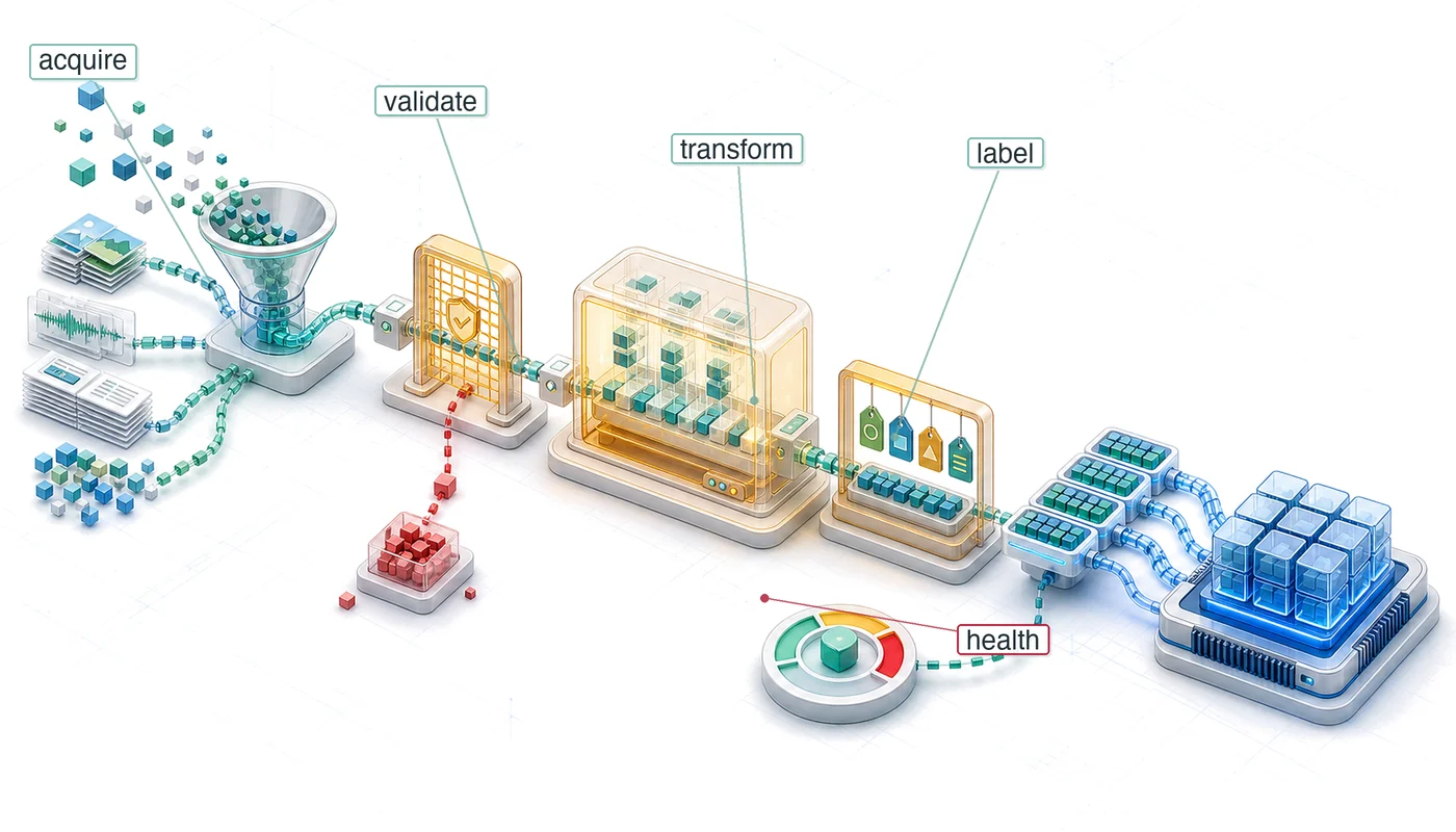
The workflow becomes concrete in the data pipeline: raw inputs pass through collection, ingestion, analysis, labeling, validation, and preparation before they become ML-ready datasets. The effort breakdown reported in the 2016 Crowdflower survey (CrowdFlower 2016) explains why that pipeline needs its own systems treatment: 60 percent of respondents selected cleaning and organizing data as their most time-consuming task, and 19 percent selected collecting datasets. The data axis of the D·A·M taxonomy becomes real only as infrastructure: acquisition systems, validation checks, labeling workflows, storage layouts, and governance.
CrowdFlower. 2016. Data Science Report 2016.
Definition 1.1: Data engineering
Data engineering is the infrastructure layer that manages the lifecycle of data from source to model, encompassing acquisition, transformation, storage, and governance.
- Significance: Its critical function is ensuring training-serving consistency, preventing silent degradation by decoupling the model from the volatility of raw data. Within the iron law, it governs bytes moved \((D_{\text{vol}})\), while dataset composition and quality determine whether the dataset \((D)\) remains representative of the target distribution.
- Distinction: Unlike data science, which focuses on inference and insight, data engineering addresses the scalability and reliability of the data pipeline.
- Common pitfall: A frequent misconception is that data engineering is “data cleaning.” In reality, it is dataset compilation: transforming raw, noisy observations into an optimized binary that the model consumes.
The dataset compilation analogy makes the infrastructure concrete. Just as a software compiler transforms source code through a series of increasingly refined representations (tokens, abstract syntax trees, intermediate representations, machine code), a data pipeline transforms raw, noisy observations into training-ready numeric tensors through analogous stages. Filtering corrupted records, outliers, and irrelevant features corresponds to dead code elimination: stripping material that contributes nothing to the learned representation. Augmentation, which synthetically expands limited examples by rotating images, pitch-shifting audio, or injecting noise, mirrors loop unrolling, exposing the model to more variations of the underlying pattern without collecting new data. Deduplication plays the role of common subexpression elimination, identifying and merging duplicate records that would otherwise bias gradient estimates and waste compute. Schema validation, enforcing strict types and ranges on every record, is the data pipeline’s type checker, rejecting malformed inputs before they crash the “runtime” of model training.
The engineering implication is that datasets must be versioned (like git), unit-tested (data quality checks), and debugged. Deleting a row of training data can change the learned artifact, just as deleting a line of code can change a compiled binary; retraining is the corresponding recompilation step. Compilation also forces a trust boundary between dataset partitions. The training set is allowed to shape parameters; the validation set is allowed to shape modeling and pipeline choices; the test set is reserved for estimating generalization after those choices have been made. Leakage occurs when information crosses those boundaries: duplicate examples appearing in multiple splits, augmented variants of the same source record landing on both sides of the split, user records from the same household appearing in both training and test, or time-derived features computed using future observations. For the keyword-spotting case study used throughout this chapter, this means speaker-independent and time-aware splits are not bookkeeping details; they are the difference between measuring memorization of familiar voices and measuring performance on the deployment population.
This compilation metaphor establishes the engineering mindset that runs through the chapter. A compiler has distinct phases (lexing, parsing, optimization, code generation), and our dataset compiler has phases too: acquisition, ingestion, processing, labeling, storage, and ongoing maintenance. A four pillars framework of Quality, Reliability, Scalability, and Governance organizes design decisions across all phases. A keyword spotting (KWS) case study illustrates each stage under extreme resource constraints, where every byte and operation matters.

Selection gain peaks where signal density (entropy) is high and movement cost (gravity) low.
Sound pipeline design begins with the physical properties that constrain each stage. Just as a civil engineer must understand soil mechanics before designing foundations, a data engineer must understand the physics of data movement and information density before making pipeline decisions. These physical constraints impose hard boundaries that no amount of clever software can circumvent.
Physics of Data
The “data as code” metaphor captures what data does (determines system behavior) but not why moving it is so expensive. The physics of data explains why data systems must treat data as a physical substance with measurable properties. Just as diverse materials have density and viscosity, datasets have task-relevant signal and data gravity.
Data gravity
Data gravity is the cost of movement. It is a function of volume \((D_{\text{vol}})\) and network bandwidth \((\text{BW})\). The time to move a petabyte dataset across a 10 Gbps link is fixed by physics (\(T = D_{\text{vol}}/\text{BW} \approx 9.3 \text{ days}\)); even a 100 Gbps dedicated link leaves transfer time and egress cost large enough to shape the architecture. This gravity dictates architecture: because moving 1 PB to the compute is slow and expensive, the compute often must move to the data. This explains the rise of “Data Lakehouse” architectures1 (Zaharia et al. 2021) where processing engines such as Spark and Presto operate over shared object storage. In contrast, data mesh (Dehghani 2022) proposes decentralizing ownership to manage this scale organizationally, treating data as a product owned by domain teams.
1 Data lakehouse: Combines data lake storage (cheap, schema-less) with warehouse query semantics (ACID transactions, schema enforcement) using transactional table layers such as Delta Lake. For ML workloads, the lakehouse reduces the extract, transform, load (ETL) copy between lake and warehouse, enabling direct feature computation on the storage layer where data already resides – a direct response to data gravity, since repeated petabyte-scale copies increase the \(D_{\text{vol}}/\text{BW}\) cost (Armbrust et al. 2020; Zaharia et al. 2021).
Armbrust, Michael, Tathagata Das, Liwen Sun, Burak Yavuz, Shixiong Zhu, Mukul Murthy, Joseph Torres, et al. 2020. “Delta Lake: High-Performance ACID Table Storage over Cloud Object Stores.” Proceedings of the VLDB Endowment 13 (12): 3411–24. https://doi.org/10.14778/3415478.3415560.
Zaharia, Matei, Ali Ghodsi, Reynold Xin, and Michael Armbrust. 2021. “Lakehouse: A New Generation of Open Platforms That Unify Data Warehousing and Advanced Analytics.” Proceedings of CIDR 8.
Dehghani, Zhamak. 2022. Data Mesh: Delivering Data-Driven Value at Scale. O’Reilly Media.
Task-relevant signal
Task-relevant signal is a heuristic for the useful information a dataset contributes to a particular task, not Shannon entropy computed from raw bytes. A dataset of 1 million identical images has high gravity but little additional task-relevant information beyond the repeated image. A dataset of 10,000 diverse edge cases may have lower gravity but greater task-relevant signal. Let this heuristic measure useful signal per byte and data gravity capture movement cost. Their ratio represents a dataset’s return on movement cost: \[ \text{Data Selection Gain} \propto \frac{\text{Task-Relevant Signal}}{\text{Data Gravity}} \tag{1}\] The heuristic favors datasets whose marginal task signal justifies their movement cost, so deduplication and active learning improve the selection decision when they remove redundant bytes or prioritize informative examples.
The feeding problem: Flow rate and the “feeding tax”
Data gravity establishes the cost of moving the entire mass; the feeding problem establishes the cost of delivering it. We analyze this as a flow rate problem: the struggle to saturate a high-throughput machine from a low-bandwidth data source.
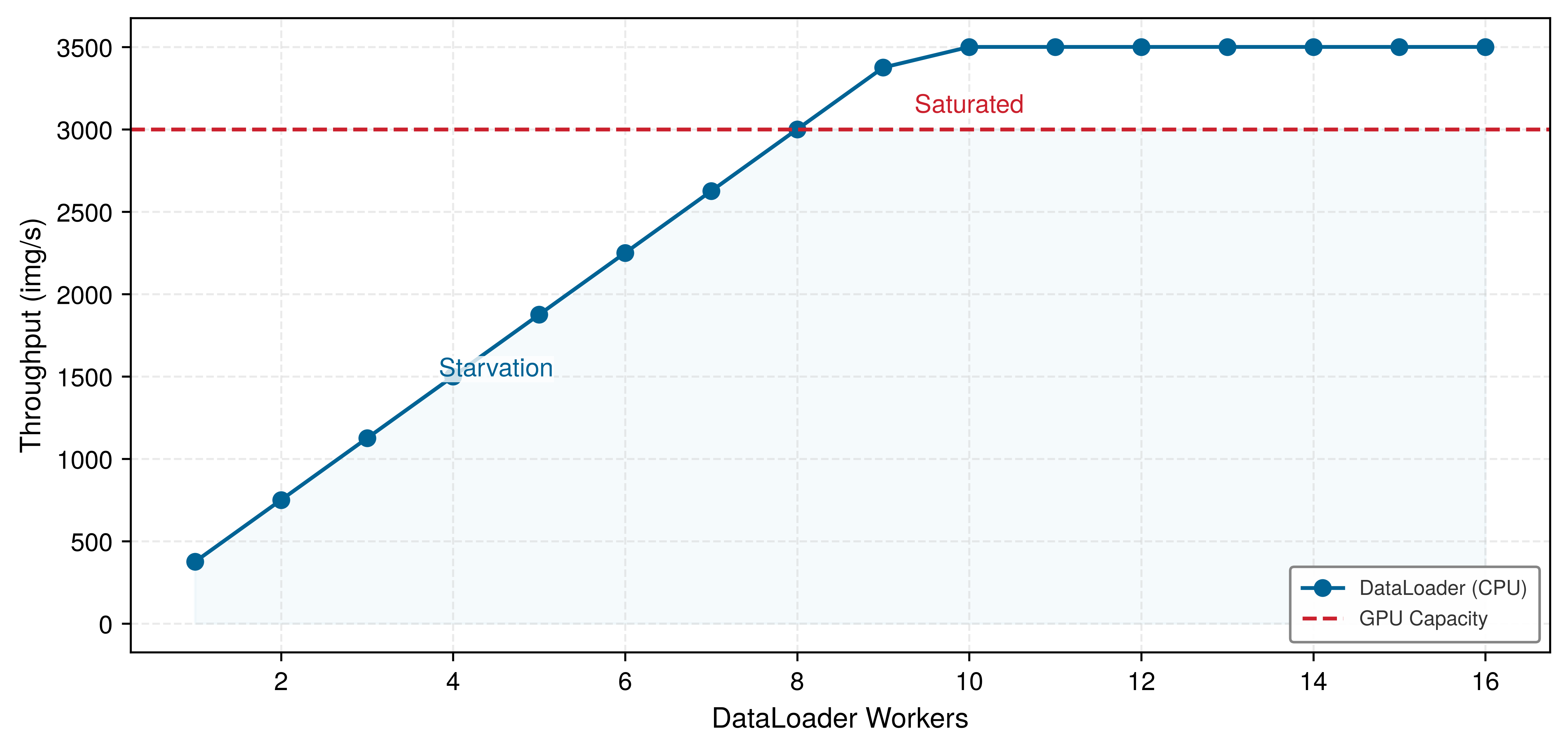
According to the iron law, the system is only as fast as its slowest term. If a high-throughput accelerator running an image model can process 1,843 img/s, but the storage pipeline delivers only 250 MB/s, the expensive silicon sits idle. We quantify this as the feeding tax: the wall-clock time lost to I/O wait, which directly reduces the system efficiency \((\eta_{\text{hw}})\) term. For a standard cloud volume, the feeding tax can exceed 77.5 percent, meaning the accelerator spends the majority of its time waiting for bits. This tax transforms the data pipeline from a simple storage concern into the primary regulator of the system’s duty cycle. Feeding the reference accelerator in this example often requires 1.1 GB/s transfer rates, forcing the shift from traditional file systems to the specialized storage architectures developed in section 1.7.1. These physical properties also carry an energy cost: as data moves farther from the processor, movement increasingly dominates the budget.
Systems Perspective 1.1: The energy-movement invariant
The iron law in Iron Law of ML Systems and the memory-wall analysis in System Balance and Hardware imply a data-engineering principle: moving one 32-bit value costs roughly 173× to 10,810.8× as much energy as the table’s FP32 multiply, with the multiplier rising as the data leaves the chip. Later optimization chapters exploit the same cost gradient inside model and hardware design; here, the question is how much energy the information flow from the external world already consumes before the model computes. Table 1 makes that cost gradient explicit across the memory hierarchy.
Table 1: Energy Cost of Moving vs. Computing on a 32-Bit Value: Approximate energy per event at each stage of the data-movement hierarchy, with multipliers normalized to one 32-bit FP32 multiply. All rows use the same 32-bit width, so the ratios compare like-sized events. They do not by themselves prove which term dominates a complete workload; total energy also depends on the number of arithmetic operations and transfers.
| Operation | Energy (pJ) | Relative Cost |
|---|---|---|
| 32-bit FP Multiply | 3.7 pJ/FLOP | 1\(\times\) |
| DRAM Memory Access (32-bit) | 640 pJ | 173× |
| Local SSD Access (32-bit) | 4,000 pJ | 1,081.1× |
| Network Transfer (32-bit) | 40,000 pJ | 10,810.8× |
The cost gradient quantified in table 1 explains why locality can be a high-leverage systems optimization. Each avoided transfer removes its associated movement energy, although the total benefit depends on access counts and reuse.
Data has physical mass. Pruning 50 percent of training data through deduplication does more than save disk space; it reduces work in data-intensive stages of the training lifecycle. Data selection is therefore a high-leverage tool when data movement and processing dominate the workload.
The energy argument and the signal-density heuristic point to the same lever from two directions: effective data engineering maximizes the Data Selection Gain defined in equation 1. “Data Cleaning” is more than basic hygiene: it is signal-to-noise engineering. Deduplication can remove redundant mass while preserving task-relevant signal, directly increasing the ratio. Active learning can prioritize informative examples over redundant ones, thereby increasing useful information per byte. We optimize this ratio to ensure our storage and compute budgets are spent on signal, not noise.
These principles operate at the level of individual files and batches. At data center scale, the cost of moving data compounds into a constraint that makes large datasets so expensive to transfer that compute must relocate to the data rather than the reverse. Transferring a petabyte dataset between data centers puts a dollar figure on the constraint.
Napkin Math 1.1: The physics of data gravity
Problem: A 1 PB training dataset resides in a US East data center, while a remote accelerator pod is available in US West. Is it faster to move the data or to move the compute?
Math:
- Network bandwidth: 100 Gb/s \(\div 8 =\) 12.5 GB/s.
- Transfer time: 1,000,000 GB \(\div\) 12.5 GB/s = 80,000 seconds, approximately
- Cost: 1,000,000 GB \(\times\) $0.02/GB = $20,000. (Baseline: AWS data transfer out pricing, 2024.)
Systems insight: If training takes less than 22 h, data transfer takes longer than training. If training costs less than $20,000 (approximately 5,000 TPUv4-hours), bandwidth costs more than compute. For petabyte-scale data, code moves to data; for gigabyte-scale data, data moves to code.
These physical constraints govern every decision in production data pipelines. Before moving on, check the fundamental intuitions that will recur throughout the pipeline.
Checkpoint 1.1: The physics of data
Data engineering is governed by physical costs. Check your intuition:
These physical properties impose hard constraints on every pipeline decision: where to store data, how to transform it, and when to move computation rather than bytes. Physics alone, however, does not prevent failures; it merely defines the boundaries within which engineering decisions must be made. A team that understands data gravity perfectly can still build a brittle pipeline if quality checks are ad hoc, error handling is absent, or governance is an afterthought. Translating physical constraints into reliable practice requires a systematic framework that organizes design decisions across every pipeline stage.
Self-Check: Question
A machine learning team maintains a \(1\text{ PB}\) raw training corpus in a US East cloud storage bucket and provisions a dedicated compute cluster in US West. The regions are connected by a dedicated \(100\text{ Gbps}\) network fabric. Cloud egress pricing is $0.02/, and the model training run takes \(20\text{ hours}\). Under the principles of data gravity and transfer economics (\(T = D_{\text{vol}}/\text{BW}\)), which architecture should the team select?
- Stream the dataset remotely across the link during training, because a 100 Gbps network provides sufficient throughput to prevent GPU I/O stalls.
- Partition the dataset equally across both cloud regions so that each region trains half the model asynchronously without transfer fees.
- Apply standard gzip compression to eliminate data gravity, enabling real-time remote streaming at zero net cost.
- Provision or relocate compute in US East near the data, because transferring 1 PB requires ~22.2 hours and incurs ~$20,000 in egress fees, exceeding the training run’s time and budget.
A computer vision model training on an accelerator cluster consumes images at \(3{,}119\text{ img/s}\), demanding \(1.9\text{ GB/s}\) of sustained input streaming bandwidth. However, the host DataLoader reads from a standard cloud block storage volume delivering only \(125\text{ MB/s}\). According to the chapter’s feeding tax analysis, what is the resulting operational state of the system?
- The accelerator suffers a feeding tax of >90% (spending over 90% of its wall-clock time idle waiting for I/O), severely degrading hardware efficiency _{}.
- The accelerator remains 100% compute-bound because internal GPU tensor execution is mathematically decoupled from storage I/O.
- Increasing the per-device batch size by 8x will completely eliminate the I/O bottleneck without requiring storage upgrades.
- Host memory caches automatically compensate for the throughput gap after the first epoch without any CPU overhead.
Using the data selection gain formula ( ) and the energy-movement invariant, explain why pruning 50% of redundant samples via deduplication provides high systems leverage even when per-batch model execution is compute-bound.
According to the chapter’s energy-movement hierarchy, arrange the following operations in ascending order of energy consumed per 32-bit value (from lowest energy to highest energy):
- Local NVMe SSD access
- On-chip 32-bit FP multiply
- Wide-area network transfer
- Off-chip DRAM memory access
- The wall-clock time lost by high-throughput accelerators while waiting for input batches from slow storage pipelines is formally termed the ____.
Four Pillars Framework
A credit scoring model rejects every applicant from a region because an upstream team changed a ZIP code field from integer to string. A medical imaging model degrades silently for months because camera hardware changed at a partner hospital. A fraud detection system misses a new attack vector because its training data was six months stale. Each failure traces to a different root cause (schema drift, distribution shift, data staleness), yet all share a common pattern: ad hoc data engineering decisions that interacted in ways no one anticipated until deployment. These cascading failures motivate a four-pillar framework organized around quality, reliability, scalability, and governance.
Data cascades
Machine learning systems face a distinctive failure pattern called data cascades, where poor data quality in early stages amplifies throughout the entire pipeline (Sambasivan et al. 2021). Some invalid inputs trigger immediate software errors, but data can also pass schemas and tests while degrading learned behavior silently2 until quality issues become severe enough to require expensive investigation, rework, or retraining.
2 Data cascades: The failure is “silent” because it degrades model inputs, not model code—corrupted data can pass unit tests and appear healthy in ordinary system monitoring. Sambasivan et al. (2021) describe cascades as often invisible and delayed: flawed data practices may surface only after downstream evaluation, deployment, or user-facing failures reveal that the model learned from the wrong signal. Remediation then requires tracing the issue back through data collection, labeling, feature engineering, and evaluation decisions, with some teams restarting or abandoning affected work.
Sambasivan, Nithya, Shivani Kapania, Hannah Highfill, Diana Akrong, Praveen Paritosh, and Lora M Aroyo. 2021. “‘Everyone Wants to Do the Model Work, Not the Data Work’: Data Cascades in High-Stakes AI.” Proceedings of the 2021 CHI Conference on Human Factors in Computing Systems, 1–15. https://doi.org/10.1145/3411764.3445518.
Data errors rarely stay confined to their point of origin; they compound across pipeline stages. Follow the sequence of connected stages in figure 1 from left to right to trace how an initial data defect propagates forward into feature extraction, model optimization, and deployment decisions.
\begin{tikzpicture}[line join=round,font=\small\sffamily]
\definecolor{Green}{HTML}{008F45}
\definecolor{Red}{HTML}{CB202D}
\definecolor{Orange}{HTML}{CC5500}
\definecolor{Blue}{HTML}{006395}
\definecolor{Violet}{HTML}{7030A0}

\tikzset{%
Line/.style={line width=1.0pt,black!50,shorten <=6pt,shorten >=8pt},
LineD/.style={line width=2.0pt,black!50,shorten <=6pt,shorten >=8pt},
Text/.style={rotate=60,align=right,anchor=north east,font=\fontsize{7pt}{8}\sffamily},
Text2/.style={align=left,anchor=north west,font=\footnotesize\sffamily,text depth=0.7}
}

\draw[line width=1.5pt,black!30](0,0)coordinate(P)--(10,0)coordinate(K);

\foreach \i in {0,...,6} {
\path let \n1 = {(\i/6)*10} in coordinate (P\i) at (\n1,0);
\fill[black] (P\i) circle (2pt);
  }

\draw[LineD,Red,overlay](P0)to[out=60,in=120](P6);
\draw[LineD,Red](P0)to[out=60,in=125](P5);
\draw[LineD,Blue](P1)to[out=60,in=120](P6);
\draw[LineD,Red](P1)to[out=50,in=125](P6);
\draw[LineD,Blue](P4)to[out=60,in=125](P6);
\draw[LineD,Blue](P3)to[out=60,in=120](P6);
%
\draw[Line,Orange](P1)to[out=44,in=132](P6);
\draw[Line,Green](P1)to[out=38,in=135](P6);
\draw[Line,Orange](P1)to[out=30,in=135](P5);
\draw[Line,Green](P1)to[out=36,in=130](P5);
%
\draw[Line,Orange](P2)to[out=40,in=135](P6);
\draw[Line,Orange](P2)to[out=40,in=135](P5);
%
\draw[draw=none,fill=VioletLine!50]($(P5)+(-0.1,0.15)$)to[bend left=10]($(P5)+(-0.1,0.61)$)--
                ($(P5)+(-0.25,0.50)$)--($(P5)+(-0.85,1.20)$)to[bend left=20]($(P5)+(-1.38,0.76)$)--
                ($(P5)+(-0.51,0.33)$)to[bend left=10]($(P5)+(-0.64,0.22)$)to[bend left=10]cycle;
\draw[draw=none,fill=VioletLine!50]($(P6)+(-0.1,0.15)$)to[bend left=10]($(P6)+(-0.1,0.61)$)--
                ($(P6)+(-0.25,0.50)$)--($(P6)+(-0.7,1.30)$)to[bend left=20]($(P6)+(-1.38,0.70)$)--
                ($(P6)+(-0.51,0.33)$)to[bend left=10]($(P6)+(-0.64,0.22)$)to[bend left=10]cycle;
%
\def\vi{-0.05}
\draw[dashed,red,thick,-latex](P1)--++(90:2)to[out=90,in=0](0.8,2.7);
\draw[dashed,red,thick,-latex](P6)--++(90:2)to[out=90,in=0](9.1,2.7);
\node[below=\vi of P0,Text]{Problem\\ Statement};
\node[below=\vi of P1,Text]{Data collection \\and labeling};
\node[below=\vi of P2,Text]{Data analysis\\ and cleaning};
\node[below=\vi of P3,Text]{Model \\selection};
\node[below=\vi of P4,Text]{Model\\ training};
\node[below=\vi of P5,Text]{Model\\ evaluation};
\node[below=\vi of P6,Text]{Model\\ deployment};
%Legend
\node[circle,minimum size=4pt,fill=Blue](L1)at(11.5,2.6){};
\node[above right=0.1 and 0.1of L1,Text2]{Interacting with physical\\  world brittleness};

\node[circle,minimum size=4pt,fill=Red,below =0.5 of L1](L2){};
\node[above right=0.1 and 0.1of L2,Text2]{Inadequate \\application-domain expertise};

\node[circle,minimum size=4pt,fill=Green,below =0.5 of L2](L3){};
\node[above right=0.1 and 0.1of L3,Text2]{Conflicting reward\\ systems};

\node[circle,minimum size=4pt,fill=Orange,below =0.5 of L3](L4){};
\node[above right=0.1 and 0.1of L4,Text2]{Poor cross-organizational\\ documentation};

\draw[-{Triangle[width=8pt,length=8pt]}, line width=3pt,Violet](11.4,-0.85)--++(0:0.8)coordinate(L5);
\node[above right=0.23 and 0of L5,Text2]{Impacts of cascades};

\draw[-{Triangle[width=4pt,length=8pt]}, line width=2pt,Red,dashed](11.4,-1.35)--++(0:0.8)coordinate(L6);
\node[above right=0.23 and 0of L6,Text2]{Abandon/re-start process};
\end{tikzpicture}Definition 1.2: Data cascade
Data cascade is an ML systems failure mode in which upstream data quality problems propagate through collection, labeling, feature engineering, training, evaluation, and deployment, amplifying into downstream model failures or user harm.
- Significance: The remediation cost scales with the number of downstream artifacts that consumed the corrupted data: feature tables must be regenerated, models retrained, evaluation metrics recomputed, and deployed systems rolled back or patched. A single schema or labeling defect can therefore invalidate an entire training run and all experiments derived from it, turning a local data error into a full-pipeline rework event.
- Distinction: Unlike an isolated data quality bug, a data cascade is defined by propagation and amplification. The initial defect may be small, but each pipeline stage treats its input as trustworthy and converts the defect into new derived state, making the root cause harder to observe as the system moves farther from collection.
- Common pitfall: A frequent misconception is that data cascades are caught by ordinary software tests. In reality, corrupted data can satisfy schemas, pass unit tests, and produce successful training jobs while teaching the model the wrong signal; preventing cascades requires lineage, validation, contracts, and monitoring tied to model behavior.
This feedback loop creates an insidious operational failure mode: silent degradation. Unlike conventional software crashes that trigger stack traces and alert pages, data-induced model errors produce syntactically valid outputs with degraded semantic accuracy. By the time downstream metrics reflect the failure, corrupted predictions have already contaminated historical data stores, forcing expensive rollbacks and data re-ingestion.
Example 1.1: The pipeline jungle
Scenario: A production credit scoring model suddenly begins rejecting all applicants from a specific geographic region.
Diagnosis: An upstream database team altered the zip_code field schema from integer to string (“02139”) to support international codes without updating downstream data contracts. A legacy downstream transform still coerced the string back to an integer before serializing it, stripping the leading zero (“2139”) and causing the model to treat a familiar postal code as an unobserved, high-risk category.
Systems lesson: Unenforced feature boundaries create pipeline jungles where upstream schema modifications cause silent downstream model failures. Versioned data contracts with strict schema and range validation prevent cross-system data corruption.
Four foundational pillars
To prevent silent failures from compounding across the pipeline, data infrastructure must balance four competing operational priorities. Observe how figure 2 organizes these priorities into foundational columns spanning input integrity, deployment stability, execution performance, and data governance.
\begin{tikzpicture}[line join=round,font=\sffamily]
\tikzset{
Box/.style={align=center, inner xsep=2pt,draw=GreenLine, line width=1pt,fill=none, minimum width=51mm, minimum height=25mm},
Circle1/.style={circle,  minimum size=33mm, draw=none, fill=BrownLine!20},
LineD/.style={dashed,BrownLine!70, line width=1.1pt,latex-latex,text=black},
LineA/.style={violet!50,line width=4.0pt,{{Triangle[width=1.5*6pt,length=2.0*5pt]}-{Triangle[width=1.5*6pt,length=2.0*5pt]}},shorten <=1pt,shorten >=1pt},
ALine/.style={black!50, line width=1.1pt,{{Triangle[width=0.9*6pt,length=1.2*6pt]}-}},
Larrow/.style={fill=violet!50, single arrow,  inner sep=2pt, single arrow head extend=3pt,
            single arrow head indent=0pt,minimum height=10mm, minimum width=3pt}
}
%%%
%vaga
\tikzset{
pics/vaga/.style = {
        code = {
        \pgfkeys{/channel/.cd, #1}
\begin{scope}[shift={($(0,0)+(0,0)$)},scale=\scalefac,every node/.append style={transform shape}]
\node[rectangle,minimum width=2mm,minimum height=22mm,
draw=none, fill=\filllcolor,line width=\Linewidth](1R) at (0,-0.95){};
\fill[fill=\filllcolor!60!black](230:2.8)arc(230:310:2.8)--cycle;%circle(2.9);
%LT
\node [semicircle, shape border rotate=180,  anchor=chord center,
      minimum size=11mm, draw=none, fill=\filllcirclecolor](LT) at (-2,-0.5) {};
\node [circle,  minimum size=4mm, draw=none, fill=\filllcirclecolor](T1) at (-2,1.25) {};
\draw[draw=\drawcolor,,line width=1.2*\Linewidth,shorten <=3pt,shorten >=3pt](T1)--(LT);
\draw[draw=\drawcolor,,line width=1.2*\Linewidth,shorten <=3pt,shorten >=3pt](T1)--(LT.30);
\draw[draw=\drawcolor,,line width=1.2*\Linewidth,shorten <=3pt,shorten >=3pt](T1)--(LT.150);
%DT
\node [semicircle, shape border rotate=180,  anchor=chord center,
      minimum size=11mm, draw=none, fill=\filllcirclecolor!70!black](DT) at (2,-0.5) {};
\node [circle,  minimum size=4mm, draw=none, fill=\filllcirclecolor!70!black](T2) at (2,1.25) {};
\draw[draw=\drawcolor,line width=1.2*\Linewidth,shorten <=3pt,shorten >=3pt](T2)--(DT);
\draw[draw=\drawcolor,,line width=1.2*\Linewidth,shorten <=3pt,shorten >=3pt](T2)--(DT.30);
\draw[draw=\drawcolor,,line width=1.2*\Linewidth,shorten <=3pt,shorten >=3pt](T2)--(DT.150);
%
\node[draw=none,rectangle,minimum width=32mm,minimum height=1.5mm,inner sep=0pt,
fill=\filllcolor!60!black]at(0,1.25){};
\node[draw=white,fill=\filllcolor,line width=2*\Linewidth,ellipse,minimum width=9mm,  minimum height=15mm](EL)at(0,0.85){};
\node[draw=white,fill=\filllcolor!60!black,line width=2*\Linewidth,,circle,minimum size=10mm](2C)at(0,2.05){};
\end{scope}
    }
  }
}
%stit
\def\inset{3.2pt} %
\def\myshape{%
  (0,1.34) to[out=220,in=0] (-1.20,1.03) --
  (-1.20,-0.23) to[out=280,in=160] (0,-1.53) to[out=20,in=260] (1.20,-0.23) --
  (1.20,1.03)  to[out=180,in=320] cycle
}
\tikzset{
pics/stit/.style = {
        code = {
        \pgfkeys{/channel/.cd, #1}
\begin{scope}[shift={($(0,0)+(0,0)$)},scale=\scalefac,every node/.append style={transform shape}]
\fill[fill=\filllcolor!60] \myshape;
%
\begin{scope}
  \clip \myshape;
  \draw[draw=\filllcolor!60, line width=2*\inset,fill=white] \myshape; % stroke color and width
\end{scope}
\fill[fill=\filllcolor!60](0,0)circle(0.4)coordinate(ST\picname);
\end{scope}
    }
  }
}
%AI style
\tikzset{
pics/llm/.style = {
        code = {
        \pgfkeys{/channel/.cd, #1}
\begin{scope}[shift={($(0,0)+(0,0)$)},scale=\scalefac,every node/.append style={transform shape}]
\node[circle,minimum size=12mm,draw=\drawcolor, fill=\filllcolor!70,line width=1.25*\Linewidth](C\picname) at (0,0){};
\def\startangle{90}
\def\radius{1.15}
\def\radiusI{1.1}
\foreach \i [evaluate=\i as \j using \i+1] [count =\k] in {0,2,4,6,8} {
\pgfmathsetmacro{\angle}{\startangle - \i * (360/8)}
\draw[draw=black,-{Circle[black ,fill=\filllcirclecolor,length=5.5pt,line width=0.5*\Linewidth]},line width=1.5*\Linewidth](C\picname)--++(\startangle - \i*45:\radius) ;
\node[circle,draw=black,fill=\filllcirclecolor!80!red!50,inner sep=3pt,line width=0.5*\Linewidth](2C\k)at(\startangle - \j*45:\radiusI) {};
}
\draw[line width=1.5*\Linewidth](2C1)--++(-0.5,0)|-(2C2);
\draw[line width=1.5*\Linewidth](2C3)--++(0.5,0)|-(2C4);
\node[circle,,minimum size=12mm,draw=\drawcolor, fill=\filllcolor!70,line width=0.5*\Linewidth]at (0,0){};
\end{scope}
    }
  }
}
%brain
\tikzset{pics/brain/.style = {
        code = {
        \pgfkeys{/channel/.cd, #1}
\begin{scope}[local bounding box=BRAIN,scale=\scalefac, every node/.append style={transform shape}]
\draw[fill=\filllcolor,line width=\Linewidth](-0.3,-0.10)to(0.08,0.60)
to[out=60,in=50,distance=3](-0.1,0.69)to[out=160,in=80](-0.26,0.59)to[out=170,in=90](-0.46,0.42)
to[out=170,in=110](-0.54,0.25)to[out=210,in=150](-0.54,0.04)
to[out=240,in=130](-0.52,-0.1)to[out=300,in=240]cycle;
\draw[fill=\filllcolor,line width=\Linewidth]
(-0.04,0.64)to[out=120,in=0](-0.1,0.69)(-0.19,0.52)to[out=120,in=330](-0.26,0.59)
(-0.4,0.33)to[out=150,in=280](-0.46,0.42)
%
(-0.44,-0.03)to[bend left=30](-0.34,-0.04)
(-0.33,0.08)to[bend left=40](-0.37,0.2) (-0.37,0.12)to[bend left=40](-0.45,0.14)
(-0.26,0.2)to[bend left=30](-0.24,0.13)
(-0.16,0.32)to[bend right=30](-0.27,0.3)to[bend right=30](-0.29,0.38)
(-0.13,0.49)to[bend left=30](-0.04,0.51);
\draw[thick,rounded corners=0.8pt,\drawcircle,-{Circle[fill=\filllcolor,length=2.5pt]}](-0.23,0.03)--(-0.15,-0.03)--(-0.19,-0.18)--(-0.04,-0.28);
\draw[thick,rounded corners=0.8pt,\drawcircle,-{Circle[fill=\filllcolor,length=2.5pt]}](-0.17,0.13)--(-0.04,0.05)--(-0.06,-0.06)--(0.14,-0.11);
\draw[thick,rounded corners=0.8pt,\drawcircle,-{Circle[fill=\filllcolor,length=2.5pt]}](-0.12,0.23)--(0.31,0.0);
\draw[thick,rounded corners=0.8pt,\drawcircle,-{Circle[fill=\filllcolor,length=2.5pt]}](-0.07,0.32)--(0.06,0.26)--(0.16,0.33)--(0.34,0.2);
\draw[thick,rounded corners=0.8pt,\drawcircle,-{Circle[fill=\filllcolor,length=2.5pt]}](-0.01,0.43)--(0.06,0.39)--(0.18,0.51)--(0.31,0.4);
\end{scope}
     }
  }
}
%graph
\tikzset{pics/graph/.style = {
        code = {
        \pgfkeys{/channel/.cd, #1}
\begin{scope}[local bounding box=GRAPH,scale=\scalefac, every node/.append style={transform shape}]
\draw[line width=2*\Linewidth,draw = \drawcolor](-0.20,0)--(2.2,0);
\draw[line width=2*\Linewidth,draw = \drawcolor](-0.20,0)--(-0.20,2.0);
\foreach \i/\vi in {0/4,0.5/8,1/12,1.5/16}{
\node[draw, minimum width  =4mm, minimum height = \vi mm, inner sep = 0pt,
      draw = \drawcolor, fill=\filllcolor!50, line width=\Linewidth,anchor=south west](COM)at(\i,0.2){};
}
%lupa
\coordinate(PO)at(1.2,0.9);
\node[circle,draw=white,line width=0.75pt,fill=\filllcirclecolor,minimum size=9mm,inner sep=0pt](LV)at(PO){};
\node[draw=none,rotate=40,rounded corners=2pt,rectangle,minimum width=2.2mm,inner sep=1pt,
fill=\filllcirclecolor,minimum height=11mm,anchor=north]at(PO){};
\node[circle,draw=none,fill=white,minimum size=5.0mm,inner sep=0pt](LM)at(PO){};
\node[font=\small\bfseries]at(LM){...};
 \end{scope}
     }
  }
}
%target
\tikzset{
pics/target/.style = {
        code = {
        \pgfkeys{/channel/.cd, #1}
\begin{scope}[shift={($(0,0)+(0,0)$)},scale=\scalefac,every node/.append style={transform shape}]
\definecolor{col1}{RGB}{62,100,125}
\definecolor{col2}{RGB}{219,253,166}
\colorlet{col1}{\filllcolor}
\colorlet{col2}{\filllcirclecolor}
\foreach\i/\col [count=\k]in {22mm/col1,17mm/col2,12mm/col1,7mm/col2,2.5mm/col1}{
\node[circle,inner sep=0pt,draw=\drawcolor,fill=\col,minimum size=\i,line width=\Linewidth](C\k){};
}
\draw[thick,fill=brown,xscale=-1](0,0)--++(111:0.13)--++(135:1)--++(225:0.1)--++(315:1)--cycle;
\path[green,xscale=-1](0,0)--(135:0.85)coordinate(XS1);
\draw[thick,fill=yellow,xscale=-1](XS1)--++(80:0.2)--++(135:0.37)--++(260:0.2)--++(190:0.2)--++(315:0.37)--cycle;
\end{scope}
    }
  }
}
%server
\tikzset {
  pics/server/.style = {
    code = {
     % \colorlet{red}{black}
\pgfkeys{/channel/.cd, #1}
      \begin{scope}[anchor=center, transform shape,scale=\scalefac, every node/.append style={transform shape}]
        \draw[draw=\drawcolor,line width=\Linewidth,fill=\filllcolor](-0.55,-0.5) rectangle (0.55,0.5);
\foreach \i in {-0.25,0,0.25} {
                \draw[line width=\Linewidth]( -0.55,\i) -- (0.55, \i);
}
        \foreach \i in {-0.375, -0.125, 0.125, 0.375} {
          \draw[line width=\Linewidth](-0.45,\i)--(0,\i);
          \fill[](0.35,\i) circle (1.5pt);
        }

        \draw[draw=\drawcolor,line width=1.5*\Linewidth](0,-0.53) |- (-0.55,-0.7);
        \draw[draw=\drawcolor,line width=1.5*\Linewidth](0,-0.53) |- (0.55,-0.7);
      \end{scope}
    }
  }
}
\pgfkeys{
  /channel/.cd,
   Depth/.store in=\Depth,
  Height/.store in=\Height,
  Width/.store in=\Width,
  filllcirclecolor/.store in=\filllcirclecolor,
  filllcolor/.store in=\filllcolor,
  drawcolor/.store in=\drawcolor,
  drawcircle/.store in=\drawcircle,
  scalefac/.store in=\scalefac,
  Linewidth/.store in=\Linewidth,
  picname/.store in=\picname,
  filllcolor=BrownLine,
  filllcirclecolor=violet!20,
  drawcolor=black,
  drawcircle=violet,
  scalefac=1,
  Linewidth=0.5pt,
  Depth=1.3,
  Height=0.8,
  Width=1.1,
  picname=C
}

\def\wi{3.5}
\node[Circle1](CI1){};
%AI
\pic[shift={(0,0)}] at  (CI1){llm={scalefac=1.2,picname=1,drawcolor=GreenD,filllcolor=GreenD!20!, Linewidth=1pt,filllcirclecolor=red}};
%brain
\pic[shift={(0.12,-0.23)}] at  (C1){brain={scalefac=1.1,picname=2,filllcolor=orange!30!, filllcirclecolor=cyan!55!black!60, Linewidth=0.75pt}};
%Quality
\node[Box,above left=1 and \wi of CI1](B1){};
\node[below=1pt of CI1,font=\sffamily\bfseries\small,align=center]{ML Data System};
\fill[green!07](B1.north west) rectangle ($(B1.north east)!0.6!(B1.south east)$)coordinate(B1DE);
\fill[green!20](B1.south east) rectangle ($(B1.north west)!0.6!(B1.south west)$)coordinate(B1LE);
\node[Box,above left=1 and \wi of CI1](){};
\tikzset{Text2/.style={font=\sffamily\bfseries\small,align=center}}
\node[Text2]at($(B1.south west)!0.5!(B1DE)$){Quality\\ {\footnotesize Accuracy \& Fitness}};
\coordinate(Q1)at($(B1.north west)!0.5!(B1DE)$);
%Quality - target
\pic[shift={(0,0)}] at  (Q1){target={scalefac=0.55,picname=1,drawcolor=BlueD,filllcolor=cyan!90!,Linewidth=0.7pt, filllcirclecolor=cyan!20}};
%Reliability - stit
\node[Box,above right=1 and \wi of CI1](B2){};
\fill[cyan!07](B2.north west) rectangle ($(B2.north east)!0.6!(B2.south east)$)coordinate(B2DE);
\fill[cyan!20](B2.south east) rectangle ($(B2.north west)!0.6!(B2.south west)$)coordinate(B2LE);
\node[Text2]at($(B2.south west)!0.5!(B2DE)$){Reliability\\ {\footnotesize Consistency \& Fault Tolerance}};
\coordinate(R1)at($(B2.north west)!0.5!(B2DE)$);
\node[Box,above right=1 and \wi of CI1,draw=BlueD](B2){};
%Reliability - stit
\pic[shift={(0,0.03)}] at  (R1){stit={scalefac=0.48,picname=1,drawcolor=orange,filllcolor=red!80!}};
\pic[shift={(0,0.03)}] at  (ST1){server={scalefac=0.52,picname=1,drawcolor= black,filllcolor=orange!30!,Linewidth=0.75pt}};
%governance
\node[Box,below left=1 and \wi of CI1](B3){};
\fill[violet!07](B3.north west) rectangle ($(B3.north east)!0.6!(B3.south east)$)coordinate(B3DE);
\fill[violet!20](B3.south east) rectangle ($(B3.north west)!0.6!(B3.south west)$)coordinate(B3LE);
\node[Text2]at($(B3.south west)!0.5!(B3DE)$){Governance\\ {\footnotesize Ethics \& Compliance}};
\coordinate(G1)at($(B3.north west)!0.5!(B3DE)$);
\node[Box,below left=1 and \wi of CI1,draw=violet](){};
%Governance - icon
\pic[shift={(-0.70,-0.6)}] at  (G1){graph={scalefac=0.6,picname=1,filllcirclecolor=RedLine,filllcolor=green!70!black, Linewidth=0.65pt}};
%Scalability - graph
\node[Box,below right=1 and \wi of CI1](B4){};
\fill[orange!07](B4.north west) rectangle ($(B4.north east)!0.6!(B4.south east)$)coordinate(B4DE);
\fill[orange!20](B4.south east) rectangle ($(B4.north west)!0.6!(B4.south west)$)coordinate(B4LE);
\node[Text2]at($(B4.south west)!0.5!(B4DE)$){Scalability\\ {\footnotesize Growth \& Performance}};
\coordinate(S1)at($(B4.north west)!0.5!(B4DE)$);
\node[Box,below right=1 and \wi of CI1,draw=OrangeLine](){};
%governance
\pic[shift={(0,0.05)}] at  (S1){vaga={scalefac=0.25,picname=1,filllcolor=BlueLine, Linewidth=0.75pt,filllcirclecolor=orange}};
%arrows
\tikzset{Text/.style={,font=\sffamily\small,align=center}}
\draw[LineD](B1)--node[above,Text]{Validation overhead vs.\\ throughput}(B2);
\draw[LineD](B1)--node[left,Text]{Bias mitigation vs.\\ data availability}(B3);
\draw[LineD](B2)--node[right,Text]{Consistency vs.\\ distributed scale}(B4);
\draw[LineD](B3)--node[below,Text]{Performance vs.\\ privacy constraints}(B4);
%
\tikzset{Text1/.style={font=\sffamily\footnotesize,align=center,text=black}}
\draw[LineA,draw=green!70!black](B1.south east)--node[below left,Text1,green!60!black]{High-quality\\ training data}(CI1);
\draw[LineA,draw=cyan!70!black](B2.south west)--node[below right,Text1,cyan!70!black]{Consistent\\ processing}(CI1);
\draw[LineA,draw=violet!80!black!40](B3.north east)--node[above left,Text1,violet]{Compliance \& \\accountability}(CI1);
\draw[LineA,draw=orange!80](B4.north west)--node[above right,Text1,orange]{Handle growing\\ data volumes}(CI1);
\end{tikzpicture}These four operational foundations establish the trade-off space for every architectural decision in this chapter. Prioritizing scalability without quality validation or reliability contracts can increase throughput while allowing bad or inconsistent data to propagate. Conversely, exhaustive governance controls can add storage and computation overhead that constrains training iteration velocity.
Reliability asks whether the same enrollment pipeline keeps working when the device, network, or user behavior is imperfect. A pipeline that produces excellent wake-word examples in a laboratory but fails during intermittent connectivity, battery pressure, or microphone glitches delivers no value in the user’s home. Error handling, retries, local buffering, and graceful degradation turn the quality rule into a usable system: the device can request another utterance, defer upload until connectivity returns, or preserve a known-good enrollment rather than silently accepting corrupted audio.
Scalability asks whether that same decision survives growth. A manual review policy that works for a thousand recordings collapses when the product expands to millions of users, dozens of languages, and long-tail acoustic conditions. The system must scale validation, storage, labeling, and retraining without letting infrastructure cost grow faster than the value of better coverage. The limiting resource therefore depends on the workload.
Lighthouse 1.1 shows where the scalability pillar bites hardest: the wall is memory capacity, and partitioning embedding tables across machines becomes a first-class design concern rather than an afterthought. Governance then defines the boundaries within which quality, reliability, and scalability may operate. For the KWS example, governance determines whether raw voice recordings may leave the device, how long enrollment audio can be retained, which consent record authorizes use, and what documentation proves that the dataset covers relevant accents without exposing private speech. A perfectly scalable, reliable, high-quality pipeline that violates the GDPR or perpetuates demographic biases creates liability rather than value. Dataset documentation practices such as data statements make part of that governance visible by recording provenance, intended use, collection conditions, and coverage needed for bias analysis and scientific comparison (Bender and Friedman 2018).
Bender, Emily M., and Batya Friedman. 2018. “Data Statements for Natural Language Processing: Toward Mitigating System Bias and Enabling Better Science.” Transactions of the Association for Computational Linguistics 6: 587–604. https://doi.org/10.1162/tacl_a_00041.
When ML systems exhibit failures, the four pillars provide a diagnostic lens for identifying root causes. Gradual accuracy degradation points to quality: data drift has shifted the serving distribution away from training, or label quality has degraded as annotator pools change. Intermittent pipeline failures point to reliability: error handling, retry logic, or resource controls are missing under peak load. Training that takes too long despite adequate hardware points to scalability: a single-threaded transformation, unpartitioned shuffle, or slow storage tier prevents parallel resources from being used. Compliance gaps discovered during audits point to governance debt: lineage tracking is incomplete, access controls are stale, or retention policies have not kept pace with regulatory changes.
Lighthouse 1.1: DLRM recommendation lighthouse
Recommendation systems built in the DLRM style exemplify the scalability challenge of modern data engineering. Modern recommendation workloads bifurcate pipeline resource demands: continuous signals stream through dense matrix pipelines, while categorical IDs demand terabyte-scale distributed lookup infrastructure. Table 2 maps these operational stress points across data ingestion, embedding table aggregation, and feature interaction stages.
Table 2: DLRM Scalability Profile: Recommendation models stress data engineering along memory capacity and sparse-access bandwidth rather than compute.
| Property | Value | System Implication |
|---|---|---|
| Data scale | High-cardinality user/item IDs | Embedding and lookup tables can outgrow one machine’s memory. |
| Constraint | Memory Capacity | The tables no longer fit on one machine and must be partitioned. |
| Bottleneck | Sparse Access | Random lookups stress memory bandwidth more than compute. |
At ingestion, high-cardinality categorical IDs remain compact records in a throughput-bound stream. The network- and memory-capacity bottleneck emerges later, when training or serving must fetch sparse embeddings from terabytes of partitioned table state. Mitigating this asymmetry requires the feature-store caching and table-partitioning strategies developed later in the pipeline lifecycle.
The most insidious failures span multiple pillars. Features that differ between training and serving implicate both quality (the values are wrong) and reliability (the computation is inconsistent). A privacy-motivated deletion policy can also create quality gaps if the retained data no longer covers the deployment population. Diagnosing such cross-pillar failures requires checking consistency contracts, comparing feature distributions across environments, and tracing transformation lineage, all techniques examined in detail throughout this chapter. Production diagnosis should therefore check data infrastructure alongside model behavior.
KWS case study
KWS systems provide an ideal case study for applying our four-pillar framework to real-world data engineering challenges. These systems power voice-activated devices like smartphones and smart speakers, detecting specific wake words such as “OK, Google” or “Alexa” within continuous audio streams while operating under strict resource constraints.3
3 Voice Match enrollment: Repeating “OK Google” creates a micro-scale data pipeline: quality filters noisy samples, reliability completes enrollment, scalability fits the model in always-on system-on-chip (SoC) memory, and governance controls storage, processing, and retention. Data engineering applies wherever data determines system behavior.
The broad operational goals of data engineering translate into concrete techniques, tools, and validation checks. For the voice assistant exchange illustrated in figure 3, these mechanisms include deduplication, schema contracts, prefetching, and lineage tracking, mapped to their corresponding architectural pillars.

The four pillars translate directly into engineering constraints for the KWS system.
The core problem is deceptively simple: detect specific keywords amidst ambient sounds and other spoken words, with high accuracy, low latency, and minimal false activations, on devices with severely limited computational resources. A well-specified problem definition identifies the desired keywords, the envisioned application, and the deployment scenario. The objectives that follow must balance competing requirements: performance targets of 98 percent accuracy in keyword detection with latency under 200 ms, alongside resource constraints demanding minimal power consumption and model sizes optimized for available device memory.
Small per-window false-positive rates compound into operational failure.
Napkin Math 1.2: False positive targets
Problem: An always-on KWS system must tolerate at most one false wake-up per month. With one-second classification windows running around the clock, how strict does the per-window false positive rate need to be?
Variables:
- Duty cycle: Always-on (24 hours/day).
- Window size: One-second classification windows.
- Windows per month: One window per second, 24 hours/day, over 30 days gives 2,592,000 windows/month.
Math:
- False positive rate (FPR): 1 tolerated false wake divided by the monthly window count gives approximately \(3.9 \times 10^{-7}\)
- Nonkeyword rejection requirement: 99.99996 percent rejection of nonkeyword windows.
Systems insight: Aggregate accuracy (for example, “99 percent accuracy”) is insufficient here. Evaluation must report false accepts per hour (FA/Hr) together with the corresponding false-rejection behavior.
Success metrics for KWS extend beyond simple accuracy to include true positive rate (correctly identified keywords relative to all spoken keywords), false positive rate (nonkeywords incorrectly identified as keywords), and detection/error trade-off curves that compare false accepts per hour against false rejection rate on streaming audio representative of real-world deployment, as demonstrated by Nayak et al. (2022). Of these metrics, the false positive rate deserves particular attention for always-on systems. Because KWS listens continuously, every second of every day, even a seemingly negligible false positive rate compounds across millions of evaluation windows. A quick calculation shows how strict that requirement becomes.
Nayak, Prateeth, Takuya Higuchi, Anmol Gupta, Shivesh Ranjan, Stephen Shum, Siddharth Sigtia, Erik Marchi, et al. 2022. “Improving Voice Trigger Detection with Metric Learning.” Interspeech 2022, 1896–900. https://doi.org/10.21437/interspeech.2022-11160.
Operational metrics further track response time (keyword utterance to system response) and power consumption (average power used during keyword detection), and stakeholder priorities create additional tension around those metrics. Device manufacturers prioritize low power consumption, software developers emphasize ease of integration, and end users demand accuracy and responsiveness. Balancing these competing requirements shapes system architecture decisions throughout development.
Embedded device constraints impose hard boundaries on these architectural choices. Memory limitations require extremely lightweight models, often in the tens-of-kilobytes range, to fit in the always-on island of the SoC;4 this constraint covers only model weights, and preprocessing code must also fit within tight memory bounds. Limited computational capabilities (often a few hundred MHz of clock speed) demand aggressive model optimization. Most embedded devices run on batteries, so KWS systems target sub-milliwatt power consumption during continuous listening. Devices must also function across diverse deployment scenarios ranging from quiet bedrooms to noisy industrial settings.
4 System-on-chip (SoC) always-on island: Modern system-on-chip designs partition power domains so a low-power “always-on” island (typically achieving sub-milliwatt draw) monitors for wake triggers while the main processor sleeps. The critical constraint is that this island must hold both the model weights and the audio preprocessing code within its dedicated SRAM—a split budget that forces KWS architectures to optimize for total footprint, not just parameter count.
Data quality and diversity ultimately determine whether these constraints can be met. The dataset must capture demographic diversity (speakers with various accents, ages, and genders) to ensure broad recognition. Keyword variations require attention since people pronounce wake words differently, and background noise diversity proves essential for training models that perform across real-world scenarios from quiet environments to noisy conditions. Once a prototype system is developed, iterative feedback and refinement keep the system aligned with objectives as deployment scenarios evolve, requiring testing in real-world conditions and systematic refinement based on observed failure patterns.
KWS design space
KWS accuracy, false-wake tolerance, latency budget, energy budget, and memory limits create a multi-dimensional design space where data engineering choices cascade through system performance. Table 3 quantifies key trade-offs, enabling principled decisions rather than ad-hoc selection. One row uses mel-frequency cepstral coefficients (MFCCs): compact speech-frequency features whose coefficient count controls feature size, compute cost, and acoustic detail; section 1.5 shows how they are extracted.
| Design Choice | Quality Impact | Latency Impact | Cost Impact | Memory Impact |
|---|---|---|---|---|
| 16 kHz vs. 8 kHz sampling | +2–4% accuracy | 2× input-processing workload | 2× raw-audio storage | 2× feature size |
| 13 vs. 40 MFCC coefficients | +3–5% accuracy | 3× feature compute | Minimal | 3× feature memory |
| 1M vs. 10M training examples | +5–8% accuracy | 10× training time | 10× labeling cost | 10× storage |
| Clean vs. noisy training data | +10–15% real-world | Minimal | 3× collection cost | Minimal |
| Local vs. cloud inference | up to 2% accuracy risk | 10 ms vs. 100 ms | $0/query vs. $0.001/query | 64 KB vs. cloud-scale |
| Synthetic vs. real augmentation | +3–5% robustness | Minimal | 10× cheaper | Minimal |
Always-on keyword spotting operates under milliwatt power envelopes and strict tens-of-kilobytes SRAM budgets. Choosing an architecture requires balancing feature resolution against memory footprint; table 3 catalogs these trade-offs across model size, inference latency, and detection accuracy for representative edge deployments.
Napkin Math 1.3: Optimizing the KWS design space
Scenario: A KWS system for a smart speaker has these constraints:
- Target: 98 percent accuracy, fewer than 1 false wake/month
- Budget: $150K total data engineering budget
- Memory: 64 KB model size limit (always-on island)
- Timeline: 6 months to production
Step 1: Apply constraints to eliminate options.
For this scenario, the team chooses two conservative options:
- 13 MFCC coefficients to reduce feature-state memory and compute
- Local inference to avoid network latency and preserve offline operation
The 64 KB model-size limit does not by itself prove that either alternative is infeasible; the deployed model, preprocessing state, runtime, and network stack require separate footprint measurements.
Step 2: Calculate budget allocation.
The $150K budget splits across three cost categories at the unit rates established in section 1.3.2:
- Labeling (~60 percent): $90K available
- Storage/Processing (~25 percent): $37.5K
- Governance/Other (~15 percent): $22.5K
At $0.10/label with 20 percent review overhead: $90K ÷ $0.12/label = 750K labeled examples
This yields roughly 0.75M labeled examples, just below the 1M anchor in our design space. The 1M-to-10M row in table 3 should therefore be read as a scaling reference rather than a direct interpolation: the real-label budget alone does not buy the full data-volume gain.
Step 3: Maximize remaining accuracy.
The quality plan has three components:
- An illustrative base-model accuracy of ~90 percent
- Partial data-volume gain from 750K real examples
- Need: higher sampling rate plus synthetic/noisy augmentation to reach the 98 percent target
Three options from the design space remain within budget and memory constraints:
- 16 kHz sampling: +2–4 percent accuracy, 2\(\times\) storage cost ✓ (fits budget)
- Noisy training data: +10–15 percent real-world accuracy, 3\(\times\) collection cost
- Synthetic augmentation: +3–5 percent robustness, 10\(\times\) cheaper than real data ✓
Step 4: Final configuration.
The scenario combines these choices with 13 MFCCs and the computed 750K real-label budget in table 4. The quality effects can overlap, so the table records a candidate configuration rather than a solved optimum.
Result: The budget calculation supports approximately 750K human-labeled examples. Reaching the 98 percent quality target and fitting the 64 KB model limit remain validation requirements for the trained and deployed system.
Systems insight: Systematic design-space analysis turns “we need more data” into a testable allocation: the stated labeling assumptions buy about 750K real examples, while synthetic volume, accuracy, and deployed footprint still require measurement.
Table 4 records the resulting configuration, pairing each design choice with the constraint that forces it: sampling and augmentation are bought where they fit the budget, while precision and memory are pinned by the always-on island.
| Choice | Selection | Rationale |
|---|---|---|
| Sampling rate | 16 kHz | +3% accuracy worth 2\(\times\) storage within budget |
| MFCC coefficients | 13 | Reduces feature-state memory and compute; final fit requires measurement |
| Training examples | 750K real + illustrative synthetic augmentation | Human-label count follows from the budget; synthetic volume is a scenario choice |
| Data diversity | Noisy + clean mix | Critical for real-world deployment |
| Inference | Local, reduced precision | Reduced precision can lower footprint; the final 64 KB fit requires the compression analysis in Model Compression |
| Augmentation | Heavy synthetic | 10\(\times\) cost efficiency |
With a candidate configuration selected from our design space, implementation requires combining multiple data collection approaches: preexisting corpora for the baseline, web scraping and crowdsourcing for coverage gaps, and synthetic generation for scale. The combination can improve coverage across diverse real-world conditions. Section 1.3 develops each of these acquisition strategies, their economics, and their KWS instantiations in full.
The four pillars provide the evaluative lens; the first concrete engineering decision is data provenance. Acquisition strategy determines the raw material that every subsequent stage refines.
Checkpoint 1.2: Four pillars framework
The four pillars provide a systems lens for every pipeline choice.
Pillars
Trade-offs
Self-Check: Question
An always-on Keyword Spotting (KWS) system on an embedded voice assistant continuously evaluates 1-second audio classification windows (\(24\text{ hours/day}\) over a \(30\text{-day}\) month). The product specification mandates an SLA of at most 1 false activation per month. An engineer suggests that achieving a standard 99% accuracy (a 1% false positive rate on background noise) is sufficient. How many false activations would a 1% FPR produce per month, and what per-window FPR is actually required?
- A 1% FPR produces 720 false activations per month; the SLA requires a per-window FPR of \(\le 1.38 \times 10^{-5}\).
- A 1% FPR produces ~25,920 false activations per month (~36 false wakes/hour); the SLA requires a per-window FPR of \(\le 3.86 \times 10^{-7}\) (>99.9999% non-keyword rejection).
- A 1% FPR produces ~2,592 false activations per month; the SLA requires a per-window FPR of \(\le 1.0 \times 10^{-4}\).
- A 1% FPR satisfies the SLA because accuracy is averaged over the total number of audio hours across the entire device fleet.
A data engineering team implements comprehensive synchronous schema and distribution validation checks directly inside the real-time event ingestion path. Under the Four Pillars framework, which primary operational trade-off will this team encounter?
- A Governance trade-off: inspecting payload schemas automatically breaches user data retention agreements.
- A Model Capacity trade-off: validating input records forces downstream neural network layers to increase parameter counts.
- A Scalability and Reliability trade-off: heavy synchronous validation consumes CPU cycles and increases per-record latency, reducing ingestion throughput and risking dropped messages during traffic spikes.
- A Durability trade-off: validating data records accelerates physical wear on persistent solid-state drive cells.
Based on the DLRM Recommendation Lighthouse, describe how modern recommendation systems bifurcate data engineering resource demands between dense continuous signals and high-cardinality categorical IDs.
True or False: Data cascades in ML systems are easily caught by standard software unit tests because corrupted input data causes deterministic assertion failures in pipeline code.
Trace the propagation sequence of a data cascade as described in the chapter, from its root cause to user-facing impact:
- Downstream model optimization on distorted representations
- Upstream sensor or schema change without contract notification
- Silent distortion of extracted features passing syntactic checks
- Degraded real-world predictions and costly post-deployment rollback
Data Acquisition
Data acquisition begins when the team names the coverage gap the model must close. The full ImageNet database5 grew to about 14.2 million labeled images across 21,841 synsets, while the ImageNet Large Scale Visual Recognition Challenge used a 1,000-class subset (Deng et al. 2009; Russakovsky et al. 2015). GPT-3’s training corpus used tens of terabytes of raw Common Crawl text filtered to hundreds of gigabytes, combined with curated web, books, and Wikipedia data (Brown et al. 2020). Our KWS system needs 23.4 million audio samples spanning 50 languages, but the challenge extends beyond raw volume. The model must recognize wake words across accents, microphones, rooms, ages, and background noises that no single collection method can economically cover. Acquisition strategy is therefore a sequence of gap-closing decisions: reuse what already matches deployment, collect what is missing, scrape or synthesize where scale is the binding constraint, and reject sources whose provenance or consent constraints make them unusable.
5 ImageNet: The 2009 paper reported 3.2 million images across 5,247 synsets; the full database later reached about 14.2 million images across 21,841 synsets, whereas the challenge used a 1,000-class subset (Deng et al. 2009, 2024; Russakovsky et al. 2015). Its value as a benchmark is inseparable from its data engineering: Fei-Fei Li’s team built labeling infrastructure that later teams could reuse. The catch is sensitivity to annotation procedures and modest distribution shifts: models tuned to ImageNet’s distribution can underperform on related but shifted test sets (Recht et al. 2019; Beyer et al. 2020).
Deng, Jia, Wei Dong, Richard Socher, Li-Jia Li, Kai Li, and Li Fei-Fei. 2009. “ImageNet: A Large-Scale Hierarchical Image Database.” 2009 IEEE Conference on Computer Vision and Pattern Recognition, 248–55. https://doi.org/10.1109/cvpr.2009.5206848.
Deng, Jia, Wei Dong, Richard Socher, Li-Jia Li, Kai Li, and Li Fei-Fei. 2024. ImageNet.
Russakovsky, Olga, Jia Deng, Hao Su, Jonathan Krause, Sanjeev Satheesh, Sean Ma, Zhiheng Huang, et al. 2015. “ImageNet Large Scale Visual Recognition Challenge.” International Journal of Computer Vision 115 (3): 211–52. https://doi.org/10.1007/s11263-015-0816-y.
Recht, Benjamin, Rebecca Roelofs, Ludwig Schmidt, and Vaishaal Shankar. 2019. “Do ImageNet Classifiers Generalize to ImageNet?” Proceedings of the 36th International Conference on Machine Learning (ICML), 5389–400.
Beyer, Lucas, Olivier J. Hénaff, Alexander Kolesnikov, Xiaohua Zhai, and Aäron van den Oord. 2020. “Are We Done with ImageNet?” arXiv Preprint arXiv:2006.07159.
The KWS case also shows why acquisition cannot optimize one pillar at a time. Achieving 98 percent accuracy across diverse acoustic environments requires representative data spanning accents, ages, and recording conditions. Maintaining consistent detection despite device variation requires recordings from different microphones and capture paths. Supporting millions of concurrent users requires volumes that manual collection cannot economically provide. Protecting user privacy in always-listening systems constrains which recordings may be retained and how they must be anonymized. A source that improves scale but weakens governance, or improves quality but excludes important speakers, does not solve the acquisition problem.
Data source evaluation and selection
The choice among curated datasets, expert crowdsourcing, controlled web scraping, and synthetic generation depends on which source best closes the next deployment-distribution gap at acceptable cost, quality, and governance risk. Evaluation therefore begins with the cheapest reusable source and escalates only when the remaining gap justifies new collection or synthesis.
Preexisting datasets from repositories such as Kaggle, UCI (Dua and Graff 2024), and ImageNet are the first test. They offer speed and comparability when the deployment distribution resembles the benchmark enough to make reuse meaningful. For KWS, a curated speech corpus can establish the baseline model and reveal which words, languages, and acoustic conditions are already covered. Its value is not guaranteed coverage; its value is that it makes the remaining gaps measurable.
Dua, Dheeru, and Casey Graff. 2024. UCI Machine Learning Repository.
Pineau, Joelle, Philippe Vincent-Lamarre, Koustuv Sinha, Vincent Larivière, Alina Beygelzimer, Florence d’Alché-Buc, Emily Fox, and Hugo Larochelle. 2021. “Improving Reproducibility in Machine Learning Research (a Report from the Neurips 2019 Reproducibility Program).” Journal of Machine Learning Research 22 (164): 1–20.
Henderson, Peter, Riashat Islam, Philip Bachman, Joelle Pineau, Doina Precup, and David Meger. 2018. “Deep Reinforcement Learning That Matters.” Proceedings of the AAAI Conference on Artificial Intelligence 32 (1): 3207–14. https://doi.org/10.1609/aaai.v32i1.11694.
Gudivada, Venkat N., Amy Apon, and Junhua Ding. 2017. “Data Quality Considerations for Big Data and Machine Learning: Going Beyond Data Cleaning and Transformations.” International Journal on Advances in Software 10 (1–2): 1–20.
That reuse decision depends on documentation quality, which directly affects reproducibility, an ongoing crisis in machine learning research (Pineau et al. 2021; Henderson et al. 2018). Good documentation captures collection methodology, variable definitions, and baseline performance, enabling validation and replication. At scale, volume and variety compound quality challenges (Gudivada et al. 2017), requiring systematic validation pipelines rather than ad-hoc inspection.
Standard validation metrics can create an illusion of model readiness when evaluated on unrepresentative data. Shared dataset usage (figure 4) illustrates how training multiple models on one common dataset propagates shared biases, blind spots, and systemic limits across an entire ecosystem.
\begin{tikzpicture}[line join=round,font=\sffamily\small]
\tikzset{%
  Box/.style={align=flush center,
    inner xsep=2pt,
    node distance=1.2,
    draw=none,%GreenLine,
    line width=0.75pt,
    fill=none,%mygreen!03,
    %text width=35mm,
    minimum width=23mm, minimum height=20mm
  },
  Box2/.style={Box, draw=none, fill=none, minimum width=17mm, minimum height=16mm
  },
  Box3/.style={Box, draw=mybrown, fill=mybrown!04, inner ysep=1pt,
  line width=0.5pt,minimum width=37mm, minimum height=5mm
  },
  Txt/.style={font=\sffamily\footnotesize,text=black
  },
  Txt2/.style={font=\sffamily\fontsize{9pt}{9}\selectfont,text=black!60,align=left,
  },
  LineA/.style={black!20,line width=1.0pt,{-{Triangle[width=1.0*4pt,length=7pt]}},shorten <=0pt,shorten >=0pt},
}

%dataS
\tikzset{%
 pics/dataS/.style = {
        code = {
        \pgfkeys{/channel/.cd, #1}
\begin{scope}[local bounding box=FUNNEL,scale=\scalefac, every node/.append style={transform shape}]
%plats
\draw[fill=\filllcolor,line width=\Linewidth,draw=\drawcolor](0,-0.3)--(-0.67,0.03)--(0,0.37)--(0.67,0.03)--cycle;
\draw[fill=\filllcirclecolor,line width=\Linewidth,draw=\drawcolor](0,0)--(-0.67,0.33)--(0,0.67)--(0.67,0.33)--cycle;
\draw[fill=\filllcolor,line width=\Linewidth,draw=\drawcolor](0,0.3)--(-0.67,0.63)--(0,0.97)--(0.67,0.63)--cycle;
%left
\draw[line width=\Linewidth,draw=\drawcolor](-0.39,1.21)--++(210:0.55)--++(270:1.22)--(-0.39,-0.56);
\fill[line width=\Linewidth,fill=\filllcirclecolor!60!violet!,draw=green,draw=\drawcolor](-0.39,1.21)circle(3pt);
\fill[line width=\Linewidth,fill=\filllcolor,draw=green,draw=\drawcolor](-0.39,-0.56)circle(3pt);
%right
\draw[line width=\Linewidth,draw=\drawcolor](0.39,1.21)--++(330:0.55)--++(270:1.22)--(0.39,-0.56);
\fill[line width=\Linewidth,fill=\filllcirclecolor!60!violet!,draw=green,draw=\drawcolor](0.39,1.21)circle(3pt);
\fill[line width=\Linewidth,fill=\filllcolor,draw=green,draw=\drawcolor](0.39,-0.56)circle(3pt);
 \end{scope}
     }
  }
}
%CPU2
\tikzset{%
 pics/cpu2/.style = {
        code = {
        \pgfkeys{/channel/.cd, #1}
\begin{scope}[local bounding box=CHIP,scale=\scalefac, every node/.append style={transform shape}]
\node[fill=\filllcolor,minimum width=15mm, minimum height=15mm,inner sep=0pt,
            rounded corners=2,outer sep=2pt] (C1) {};
\node[fill=white,minimum width=11mm, minimum height=11mm,inner sep=0pt,] (C2) {};
\node[fill=\filllcolor!40,minimum width=7mm, minimum height=7mm,inner sep=0pt,] (C3) {};
\foreach \x in {0.2,0.5,0.8}{
\draw[line width=2*\Linewidth,draw=\drawcolor,
-{Circle[fill=white,length=4.5pt]}]($(C1.north west)!\x!(C1.north east)$)--++(0,7mm);
}
\foreach \x in {0.2,0.5,0.8}{
\draw[line width=2*\Linewidth,draw=\drawcolor,
-{Circle[fill=white,length=4.5pt]}]($(C1.south west)!\x!(C1.south east)$)--++(0,-7mm);
}
\foreach \x in {0.2,0.5,0.8}{
\draw[line width=2*\Linewidth,draw=\drawcolor,
-{Circle[fill=white,length=4.5pt]}]($(C1.north west)!\x!(C1.south west)$)--++(-7mm,0);
}
\foreach \x in {0.2,0.5,0.8}{
\draw[line width=2*\Linewidth,draw=\drawcolor,
-{Circle[fill=white,length=4.5pt]}]($(C1.north east)!\x!(C1.south east)$)--++(7mm,0);
}
 \end{scope}
     }
  }
}
%Hand
\tikzset {
pics/hand/.style = {
        code = {
        \pgfkeys{/channel/.cd, #1}
\begin{scope}[local bounding box=MOB,scale=\scalefac, every node/.append style={transform shape}]
\draw[draw=\drawcolor,line width=\Linewidth,fill=\filllcirclecolor](1.07,-0.02)--(1.70,0.2)arc(110:-40:1.0mm)--
(1.0,-0.48)arc(-60:-100:4.0mm)--(0.4,-0.34)--(0.15,-0.42)
--(-0.1,0.13)--(0.31,0.33)--(1,0.08);to [bend left=25]cycle;
\draw[draw=\drawcolor,line width=\Linewidth](-0.1,0.13)--(0.31,0.33)--(1,0.08)arc(60:-90:1.4mm)--(0.55,-0.03);
\node[draw=\drawcolor,line width=\Linewidth,fill=cyan ,minimum width=8mm,minimum height=5mm,rotate=117]at(-0.17,-0.26){};
 \end{scope}
     }
  }
}
%globe
\tikzset{
pics/globe/.style = {
        code = {
        \pgfkeys{/channel/.cd, #1}
\begin{scope}[shift={($(0,0)+(0,0)$)},scale=\scalefac,every node/.append style={transform shape}]
\node[circle,minimum size=25mm,draw=\drawcolor, fill=\filllcolor!70,line width=\Linewidth](C\picname) at (0,0){};
\draw[draw=\drawcolor,line width=\Linewidth](C\picname.north)to[bend left=65](C\picname.south);
\draw[draw=\drawcolor,line width=\Linewidth](C\picname.north)to[bend right=65](C\picname.south);
\draw[draw=\drawcolor,line width=\Linewidth](C\picname.north)to(C\picname.south);
\draw[draw=\drawcolor,line width=\Linewidth](C\picname.west)--(C\picname.east);
%
\draw[draw=\drawcolor,line width=\Linewidth](C\picname.130)to[bend right=35](C\picname.50);
\draw[draw=\drawcolor,line width=\Linewidth](C\picname.230)to[bend left=35](C\picname.310);
%\draw[red,line width=2*\Linewidth,
%,{-{Triangle[width=1.0*5pt,length=9pt]}}](C\picname.south) arc[start angle=270, end angle=360, radius=12mm];
%\draw[red,line width=2*\Linewidth,
%,{-{Triangle[width=1.0*5pt,length=9pt]}}](C\picname.south) arc[start angle=270, end angle=180, radius=12mm];
\end{scope}
    }
  }
}

\pgfkeys{
  /channel/.cd,
   Depth/.store in=\Depth,
  Height/.store in=\Height,
  Width/.store in=\Width,
  filllcirclecolor/.store in=\filllcirclecolor,
  filllcolor/.store in=\filllcolor,
  drawcolor/.store in=\drawcolor,
  drawcircle/.store in=\drawcircle,
  scalefac/.store in=\scalefac,
  Linewidth/.store in=\Linewidth,
  picname/.store in=\picname,
  filllcolor=BrownLine,
  filllcirclecolor=violet!20,
  drawcolor=black,
  drawcircle=violet,
  scalefac=1,
  Linewidth=0.5pt,
  Depth=1.3,
  Height=0.8,
  Width=1.1,
  picname=C
}

% Central
\node[Box](B1){};
\coordinate(GO1)at($(B1.north west)!0.38!(B1.north east)$);
%\fill[fill=BlueL!90](B1.south west)rectangle(GO1);
\coordinate(T1)at($(GO1)!0.5!(B1.south east)$);
\coordinate(I1)at($(B1.west)!0.21!(B1.east)$);
%\node[align=center]at(T1){Model\\ Training};
\draw[myblue,  line width=2.75pt](B1.south west)--coordinate[pos=0.5](SR1)(B1.south east);
\node[anchor=north,below=2pt of SR1](TG){Central Training Dataset Repository};
\pic[shift={(0,-0.3)}] at  (B1){dataS={scalefac=0.8,Linewidth=1.0pt,
 filllcolor=cyan!90!black!40!,drawcolor=black,filllcirclecolor=orange}};
%%%%%%%%%%%%%%%%%%
%Models
%%%%%%%%%%%%%%%%%%
\node[Box2,below=1.70 of B1](B2){};
\draw[mygreen,  line width=2.75pt](B2.south west)--coordinate[pos=0.5](SR2)(B2.south east);
\node[Box2,right= 1.55 of B2](B3){};
\draw[mygreen,  line width=2.75pt](B3.south west)--coordinate[pos=0.5](SR3)(B3.south east);
\node[Box2,right=1.55  of B3](B4){};
\draw[mygreen,  line width=2.75pt](B4.south west)--coordinate[pos=0.5](SR4)(B4.south east);
%
\node[Box2,left=1.55  of B2](B5){};
\draw[mygreen,  line width=2.75pt](B5.south west)--coordinate[pos=0.5](SR5)(B5.south east);
\node[Box2,left=1.55  of B5](B6){};
\draw[mygreen,  line width=2.75pt](B6.south west)--coordinate[pos=0.5](SR6)(B6.south east);

\foreach \i  [count=\k from 2] in {C,D,E,B,A}{
\node[anchor=north,below=2pt of SR\k](T\i){Model \i};
  }

\foreach \i  in{2,3,4,5,6}{
  \pic[shift={(0,0)}] at  (B\i){cpu2={scalefac=0.4,drawcolor=myblue, filllcolor=myblue, Linewidth=0.5pt}};
  }
 %%%%%%%%%%%%%%%%
 \node[Box,below=2 of B2](B7){};
 \draw[Dandelion,  line width=2.75pt](B7.south west)--coordinate[pos=0.5](SR7)(B7.south east);
 \node[anchor=north,below=2pt of SR7](TDO){Limited Real-World Alignment};
 \pic[shift={(-0.6,-0.30)},rotate=0] at (B7){hand={scalefac=0.8,filllcolor=orange!30!, filllcirclecolor=brown!60, Linewidth=1.0pt}};
\pic[shift={(0.3,0.4)}] at  (B7){globe={scalefac=0.35,picname=1,filllcolor=cyan!30!, Linewidth=0.75pt}};
%%
%\node[Box3,Txt](BB1)at($(TG.south)!0.43!(B2.north)$){Shared training data};

%arrows
%\draw[LineA,shorten <=-3pt](TG)--(BB1);
\foreach \i  in{2,3,4,5,6}{
\draw[LineA,shorten >=-4pt](TG)--coordinate[pos=0.4](GT\i)++(0,-10mm)-|(B\i.north);
}

 \node[Txt2,right=1pt of GT2] {Shared training data};

\foreach \i /\x in {%
A/{Bias\\ propagation},
B/{Shared\\ limits},
C/{Blind\\ spots},
D/{Common\\Weaknesses},
E/Systemic\\ issues
}{
\draw[LineA,shorten >=-4pt](T\i)--node[Txt2,pos=0.45,right](MT){\x}++(0,-12mm)-|(B7.90);
}

\node[draw=myorange,dashed,thick,fit=(B6)(B4)(TDO)(MT),inner ysep=2mm,,inner xsep=1mm,xshift=-1mm,yshift=2.7mm](BB2){};
\node[myorange,anchor=south east,above left=0.2 of BB2.south east]{Potential Issues};
\end{tikzpicture}This distribution gap represents the primary risk of static offline benchmarks. Because loss functions only optimize over observed samples, models exploit spurious artifacts present in training sets that disappear in production environments, making automated drift monitoring and continuous data validation mandatory operational requirements.
Scalability and cost optimization
Quality-focused data acquisition approaches face inherent scaling limitations. When scale requirements dominate, needing millions or billions of examples that manual curation cannot economically provide, web scraping and synthetic generation offer paths to massive datasets. Data-acquisition scalability requires understanding the economic models underlying different acquisition strategies: cost per labeled example, throughput limitations, and how these scale with data volume. Cost-effectiveness inverts with scale: what works at thousands of examples becomes prohibitive at millions, while high-setup-cost approaches amortize favorably at large volumes.
The per-unit economics at each stage determine which strategy dominates. Labeling a single medical image, for example, can cost orders of magnitude more than storing it for a year, a ratio that reshapes budget allocation for any team operating under fixed funding. Table 5 and table 6 provide essential context for acquisition decisions.
ML engineers should use the dated reference assumptions in table 5 and table 6 as inputs to workload-specific comparisons, not as current price quotes or directly comparable totals.
| Operation | Cost | Notes |
|---|---|---|
| Crowdsourced image label | $0.01–0.05 | Simple classification |
| Bounding box annotation | $0.05–0.20 | Per box, simple scenes |
| Expert medical label | $50–200 | Per study, radiologist |
| S3 storage (Standard) | $23/TB/month | Hot storage |
| S3 retrieval (Glacier) | $0.02/GB | Standard: 3-5 hours |
| Cloud GPU training hour | $2–4 | Cloud spot pricing |
| Human review hour | $15–50 | Depending on expertise |
Table 6 extends the picture with illustrative durations for labeling, training, and serving operations.
| Operation | Duration | Bottleneck |
|---|---|---|
| Label 1M images (crowdsourced) | 2–4 weeks | Annotation throughput |
| Train ResNet-50 on ImageNet | 4–6 hours | Compute (8\(\times\) A100, optimized) |
| Feature store lookup | 1–10 ms | Network + cache |
The contrast in this illustrative scenario matters: weeks for human labeling, hours for GPU training, milliseconds for serving. Here, labeling is the bottleneck. A $100K labeling budget compares with $64–$192 for one 8\(\times\) A100 ResNet-50 run, a 520.8×–1,562.5× ratio. Within that labeling spend, the assumed effort distribution is itself skewed: 80 percent of the work goes to 20 percent of features—the long tail of edge cases, rare categories, and quality exceptions.
All cost figures reflect approximate 2024 cloud provider rates and are intended to convey relative magnitudes rather than exact pricing.6 For this workload and cost model, human labor dominates the cost of a single training run. Other tasks, especially those that reuse existing labels or require repeated large-scale training, can have a different dominant term; teams should measure before deciding where to optimize.
6 Pricing ratios: Archive-retrieval prices and tier ratios reflect provider policy, not a physical invariant. In this illustrative scenario, expedited retrieval costs three times the standard tier; actual prices and tier availability must be verified before deployment.
Kuznetsova, Alina, Hassan Rom, Neil Alldrin, Jasper Uijlings, Ivan Krasin, Jordi Pont-Tuset, Shahab Kamali, et al. 2020. “The Open Images Dataset V4: Unified Image Classification, Object Detection, and Visual Relationship Detection at Scale.” International Journal of Computer Vision 128 (7): 1956–81. https://doi.org/10.1007/s11263-020-01316-z.
Groeneveld, Dirk, Iz Beltagy, Pete Walsh, Akshita Bhagia, Rodney Kinney, Oyvind Tafjord, Ananya Harsh Jha, et al. 2024. “OLMo: Accelerating the Science of Language Models.” Proceedings of the 62nd Annual Meeting of the Association for Computational Linguistics (Volume 1: Long Papers), 15789–809. https://doi.org/10.18653/v1/2024.acl-long.841.
Chen, Mark, Jerry Tworek, Heewoo Jun, Qiming Yuan, Henrique Ponde de Oliveira Pinto, Jared Kaplan, Harri Edwards, et al. 2021. “Evaluating Large Language Models Trained on Code.” arXiv Preprint arXiv:2107.03374.
Web scraping is the first lever on that cost structure, enabling dataset construction at scales that manual curation cannot match. Major vision datasets like ImageNet (Deng et al. 2024) and OpenImages (Kuznetsova et al. 2020) were built through systematic scraping, and large language models depend on web-scale text corpora (Groeneveld et al. 2024). Targeted scraping of domain-specific sources, such as code repositories (Chen et al. 2021), further demonstrates the approach’s versatility. However, production systems that rely on continuous scraping face pipeline reliability challenges: website structure changes break extractors, rate limiting throttles collection throughput, and dynamic content introduces inconsistencies that degrade model performance. Scraped results can also include historical images for contemporary queries, requiring systematic validation and cleaning.
Figure 5 shows one such result from a web scrape for “traffic light”: a historical photograph rather than a modern LED signal. If images from this context were overrepresented or correlated with a label, a model could learn spurious cues involving uniformed officers or historical streets rather than the visual properties required in its deployment environment.
Stromberg, Joseph. 2015. When Was the First Traffic Light Installed? Today in 1914. Vox.
This example reveals why the quality pillar cannot be satisfied by scale alone: no amount of additional scraped data removes the need for validation that detects and filters anachronistic or contextually inappropriate content. Beyond technical quality challenges, legal and ethical constraints further bound what scraping can achieve. Not all websites permit scraping, and ongoing litigation around training data usage illustrates the legal uncertainty and potential consequences (Harvard Law School 2024). Teams must document data provenance, ensure compliance with terms of service and copyright law, and apply anonymization procedures when scraping user-generated content.
Harvard Law School. 2024. Does ChatGPT Violate New York Times Copyrights?
Amazon Web Services. 2024. Amazon Mechanical Turk.
Sheng, Victor S., and Jing Zhang. 2019. “Machine Learning with Crowdsourcing: A Brief Summary of the Past Research and Future Directions.” Proceedings of the AAAI Conference on Artificial Intelligence 33 (01): 9837–43. https://doi.org/10.1609/aaai.v33i01.33019837.
7 Amazon Mechanical Turk (MTurk): A crowdsourcing platform that routes small tasks to distributed workers and can scale annotation beyond expert-only workflows. Snow et al. (2008) evaluate this pattern for natural-language annotation tasks, showing that non-expert annotations can be useful when task design and quality control are handled carefully. For wake-word audio collection, the same systems trade-off appears in domain-specific form: scale is attractive, but submissions still need acoustic checks such as signal-to-noise ratio, duration, and recording validity before they can safely enter the training set.
Snow, Rion, Brendan O’Connor, Daniel Jurafsky, and Andrew Y. Ng. 2008. “Cheap and Fast—but Is It Good? Evaluating Non-Expert Annotations for Natural Language Tasks.” Proceedings of the Conference on Empirical Methods in Natural Language Processing - EMNLP ’08, 254. https://doi.org/10.3115/1613715.1613751.
Crowdsourcing shifts the acquisition bottleneck from finding enough examples to controlling the quality of many parallel judgments. Platforms like Amazon Mechanical Turk (Amazon Web Services 2024) demonstrated this at landmark scale with ImageNet, where distributed contributors categorized millions of images into thousands of classes (Deng et al. 2024). Crowdsourcing offers two systems advantages: scalability through parallel microtask distribution, and diversity through the range of perspectives, cultural contexts, and linguistic variations that a global contributor pool introduces. This diversity can improve generalization when it broadens coverage of the deployment population. The cost is that task design, validation, and iteration become part of the acquisition system: tasks can be adjusted dynamically based on initial results, enabling refinement of collection strategies as quality gaps emerge (Sheng and Zhang 2019). For our KWS system, MTurk-style platforms7 enable targeted collection of wake word samples across different demographics and environments, an approach particularly valuable for underrepresented languages or specific acoustic conditions.
Moving beyond human-generated data entirely, synthetic data generation changes the scaling constraint: examples can be generated algorithmically, but their value depends on whether the generator covers the deployment conditions that real collection would miss. This approach changes the economics of data acquisition by reducing human labor while increasing the burden on validation. The pipeline in figure 6 shows synthetic and historical data entering the same training workflow.
\begin{tikzpicture}[line join=round,font=\sffamily\small]
\tikzset{
 Line/.style={line width=0.35pt,black!50,text=black},
 LineDO/.style={single arrow, draw=VioletLine, fill=VioletLine!50,
      minimum width = 10pt, single arrow head extend=3pt,
      minimum height=15mm},
 ALineA/.style={violet!80!black!50,line width=3pt,shorten <=2pt,shorten >=2pt,
{Triangle[width=1.1*6pt,length=0.8*6pt]}-{Triangle[width=1.1*6pt,length=0.8*6pt]}},
LineD/.style={line width=0.75pt,black!50,text=black,dashed,dash pattern=on 5pt off 3pt},
Circle/.style={inner xsep=2pt,
  % node distance=1.15,
  circle,
    draw=BrownLine,
    line width=0.75pt,
    fill=BrownL!40,
    minimum size=18mm
  },
 circles/.pic={
\pgfkeys{/channel/.cd, #1}
\node[circle,draw=\channelcolor,line width=\Linewidth,fill=\channelcolor!10,
minimum size=2.5mm](\picname){};
        }
}
\tikzset {
pics/cloud/.style = {
        code = {
\colorlet{red}{RedLine}
\begin{scope}[local bounding box=CLO,scale=0.5, every node/.append style={transform shape},,shift={($(SIM)+(0,0)$)},]
\draw[red,fill=white,line width=0.9pt](0.67,1.21)to[out=55,in=90,distance=13](1.5,0.96)
to[out=360,in=30,distance=9](1.68,0.42);
\draw[red,fill=white,line width=0.9pt](0,0)to[out=170,in=180,distance=11](0.1,0.61)
to[out=90,in=105,distance=17](1.07,0.71)
to[out=20,in=75,distance=7](1.48,0.36)
to[out=350,in=0,distance=7](1.48,0)--(0,0);
\draw[red,fill=white,line width=0.9pt](0.27,0.71)to[bend left=25](0.49,0.96);

\end{scope}
     }
  }
}
%streaming
\tikzset{%
 LineST/.style={-{Circle[\channelcolor,fill=RedLine,length=4pt]},draw=\channelcolor,line width=\Linewidth,rounded corners},
 ellipseST/.style={fill=\channelcolor,ellipse,minimum width = 2.5mm, inner sep=2pt, minimum height =1.5mm},
 BoxST/.style={line width=\Linewidth,fill=white,draw=\channelcolor,rectangle,minimum width=56,
 minimum height=16,rounded corners=1.2pt},
 pics/streaming/.style = {
        code = {
        \pgfkeys{/channel/.cd, #1}
\begin{scope}[local bounding box=STREAMING,scale=\scalefac, every node/.append style={transform shape}]
\node[BoxST,minimum width=44,minimum height=48](\picname-RE1){};
\foreach \i/\j in{1/north,2/center,3/south}{
\node[BoxST](\picname-GR\i)at(\picname-RE1.\j){};
\node[ellipseST]at($(\picname-GR\i.west)!0.2!(\picname-GR\i.east)$){};
\node[ellipseST]at($(\picname-GR\i.west)!0.4!(\picname-GR\i.east)$){};
}
\draw[LineST](\picname-GR3)--++(2,0)coordinate(\picname-C4);
\draw[LineST](\picname-GR3.320)--++(0,-0.7)--++(0.8,0)coordinate(\picname-C5);
\draw[LineST](\picname-GR3.220)--++(0,-0.7)--++(-0.8,0)coordinate(\picname-C6);
\draw[LineST](\picname-GR3)--++(-2,0)coordinate(\picname-C7);
 \end{scope}
     }
  }
}
%data
\tikzset{mycylinder/.style={cylinder, shape border rotate=90, aspect=1.3, draw, fill=white,
minimum width=25mm,minimum height=11mm,line width=\Linewidth,node distance=-0.15},
pics/data/.style = {
        code = {
        \pgfkeys{/channel/.cd, #1}
\begin{scope}[local bounding box=STREAMING,scale=\scalefac, every node/.append style={transform shape}]
\node[mycylinder,fill=\channelcolor!50] (A) {};
\node[mycylinder, above=of A,fill=\channelcolor!30] (B) {};
\node[mycylinder, above=of B,fill=\channelcolor!10] (C) {};
 \end{scope}
     }
  }
}

\tikzset{pics/brain/.style = {
        code = {
        \pgfkeys{/channel/.cd, #1}
\begin{scope}[local bounding box=BRAIN,scale=\scalefac, every node/.append style={transform shape}]
\fill[fill=\filllcolor!50](0.1,-0.5)to[out=0,in=180](0.33,-0.5)
to[out=0,in=270](0.45,-0.38)to(0.45,-0.18)
to[out=40,in=240](0.57,-0.13)to[out=110,in=310](0.52,-0.05)
to[out=130,in=290](0.44,0.15)to[out=90,in=340,distance=8](0.08,0.69)
to[out=160,in=80](-0.42,-0.15)to (-0.48,-0.7)to(0.07,-0.7)to(0.1,-0.5)
(-0.10,-0.42)to[out=310,in=180](0.1,-0.5);
\draw[draw=\drawchannelcolor,line width=\Linewidth](0.1,-0.5)to[out=0,in=180](0.33,-0.5)
to[out=0,in=270](0.45,-0.38)to(0.45,-0.18)
to[out=40,in=240](0.57,-0.13)to[out=110,in=310](0.52,-0.05)
to[out=130,in=290](0.44,0.15)to[out=90,in=340,distance=8](0.08,0.69)
(-0.42,-0.15)to (-0.48,-0.7)
(0.07,-0.7)to(0.1,-0.5)
(-0.10,-0.42)to[out=310,in=180](0.1,-0.5);
%brain
\draw[fill=\filllcolor,line width=\Linewidth](-0.3,-0.10)to(0.08,0.60)
to[out=60,in=50,distance=3](-0.1,0.69)to[out=160,in=80](-0.26,0.59)to[out=170,in=90](-0.46,0.42)
to[out=170,in=110](-0.54,0.25)to[out=210,in=150](-0.54,0.04)
to[out=240,in=130](-0.52,-0.1)to[out=300,in=240](-0.3,-0.10);
\draw[fill=\filllcolor,line width=\Linewidth]
(-0.04,0.64)to[out=120,in=0](-0.1,0.69)(-0.19,0.52)to[out=120,in=330](-0.26,0.59)
(-0.4,0.33)to[out=150,in=280](-0.46,0.42)
%
(-0.44,-0.03)to[bend left=30](-0.34,-0.04)
(-0.33,0.08)to[bend left=40](-0.37,0.2) (-0.37,0.12)to[bend left=40](-0.45,0.14)
(-0.26,0.2)to[bend left=30](-0.24,0.13)
(-0.16,0.32)to[bend right=30](-0.27,0.3)to[bend right=30](-0.29,0.38)
(-0.13,0.49)to[bend left=30](-0.04,0.51);

\draw[rounded corners=0.8pt,\drawcircle,-{Circle[fill=\filllcirclecolor,length=2.5pt]}](-0.23,0.03)--(-0.15,-0.03)--(-0.19,-0.18)--(-0.04,-0.28);
\draw[rounded corners=0.8pt,\drawcircle,-{Circle[fill=\filllcirclecolor,length=2.5pt]}](-0.17,0.13)--(-0.04,0.05)--(-0.06,-0.06)--(0.14,-0.11);
\draw[rounded corners=0.8pt,\drawcircle,-{Circle[fill=\filllcirclecolor,length=2.5pt]}](-0.12,0.23)--(0.31,0.0);
\draw[rounded corners=0.8pt,\drawcircle,-{Circle[fill=\filllcirclecolor,length=2.5pt]}](-0.07,0.32)--(0.06,0.26)--(0.16,0.33)--(0.34,0.2);
\draw[rounded corners=0.8pt,\drawcircle,-{Circle[fill=\filllcirclecolor,length=2.5pt]}](-0.01,0.43)--(0.06,0.39)--(0.18,0.51)--(0.31,0.4);
\end{scope}
     }
  }
}

\tikzset{pics/tube/.style = {
        code = {
        \pgfkeys{/channel/.cd, #1}
\begin{scope}[local bounding box=BRAIN,scale=\scalefac, every node/.append style={transform shape}]
\draw[draw=\drawchannelcolor,line width=\Linewidth,fill=white](-0.1,0.26)to(-0.1,0.1)to[out=240,in=60](-0.23,-0.14)
to[out=240,in=180,distance=3](-0.13,-0.27)to(0.09,-0.27)
to[out=0,in=300,distance=3](0.19,-0.14)
to[out=120,in=290]((0.06,0.1)to(0.06,0.26)
to cycle;
\fill[fill=\filllcolor!50](-0.23,-0.14)
to[out=240,in=180,distance=3](-0.13,-0.27)to(0.09,-0.27)
to[out=0,in=300,distance=3](0.19,-0.14)to[out=200,in=20]cycle;
\draw[draw=\drawchannelcolor,line width=\Linewidth,fill=none](-0.1,0.26)to(-0.1,0.1)to[out=240,in=60](-0.23,-0.14)
to[out=240,in=180,distance=3](-0.13,-0.27)to(0.09,-0.27)
to[out=0,in=300,distance=3](0.19,-0.14)
to[out=120,in=290]((0.06,0.1)to(0.06,0.26)
to cycle;
\end{scope}
     }
  }
}

\tikzset{pics/factory/.style = {
        code = {
        \pgfkeys{/channel/.cd, #1}
\begin{scope}[local bounding box=FACTORY,scale=\scalefac, every node/.append style={transform shape}]
\node[rectangle,draw=\drawchannelcolor,fill=\filllcolor!50,minimum height=15,minimum width=23,,line width=\Linewidth](R1){};
\draw[fill=\filllcolor!50,line width=1.0pt]($(R1.40)+(0,-0.01)$)--++(110:0.2)--++(180:0.12)|-($(R1.40)+(0,-0.01)$);
\draw[line width=\Linewidth,fill=green](-0.68,-0.27)--++(88:0.85)--++(0:0.15)--(-0.48,-0.27)--cycle;
\draw[line width=2.5pt](-0.8,-0.27)--(0.55,-0.27);

\foreach \x in{0.25,0.45,0.65}{
\node[rectangle,fill=black,minimum height=2,minimum width=5,thick,inner sep=0pt]
at ($(R1.north)!\x!(R1.south)$){};
}
\foreach \x in{0.25,0.45,0.65}{
\node[rectangle,fill=black,minimum height=2,minimum width=5,thick,inner sep=0pt]
at ($(R1.130)!\x!(R1.230)$){};
}
\foreach \x in{0.25,0.45,0.65}{
\node[rectangle,fill=black,minimum height=2,minimum width=5,thick,inner sep=0pt]
at ($(R1.50)!\x!(R1.310)$){};
}
\end{scope}
     }
  }
}

\tikzset {
pics/cloud/.style = {
        code = {
\colorlet{red}{BrownLine}
\pgfkeys{/channel/.cd, #1}
\begin{scope}[local bounding box=CLO,scale=\scalefac, every node/.append style={transform shape}]
\draw[red,line width=\Linewidth,fill=red!10](0,0)to[out=170,in=180,distance=11](0.1,0.61)
to[out=90,in=105,distance=17](1.07,0.71)
to[out=20,in=75,distance=7](1.48,0.36)
to[out=350,in=0,distance=7](1.48,0)--(0,0);
\draw[red,line width=\Linewidth](0.27,0.71)to[bend left=25](0.49,0.96);
%\draw[red,line width=\Linewidth](0.67,1.21)to[out=55,in=90,distance=13](1.5,0.96)
%to[out=360,in=30,distance=9](1.68,0.42);
\end{scope}
     }
  }
}
\tikzset{
pics/square/.style = {
        code = {
        \pgfkeys{/channel/.cd, #1}
\begin{scope}[local bounding box=SQUARE,scale=\scalefac,every node/.append style={transform shape}]
% Right Face
\draw[fill=\channelcolor!70,line width=\Linewidth]
(\Depth,0,0)coordinate(\picname-ZDD)--(\Depth,\Width,0)--(\Depth,\Width,\Height)--(\Depth,0,\Height)--cycle;
% Front Face
\draw[fill=\channelcolor!40,line width=\Linewidth]
(0,0,\Height)coordinate(\picname-DL)--(0,\Width,\Height)coordinate(\picname-GL)--
(\Depth,\Width,\Height)coordinate(\picname-GD)--(\Depth,0,\Height)coordinate(\picname-DD)--(0,0,\Height);
% Top Face
\draw[fill=\channelcolor!20,line width=\Linewidth]
(0,\Width,0)coordinate(\picname-ZGL)--(0,\Width,\Height)coordinate(\picname-ZGL)--
(\Depth,\Width,\Height)--(\Depth,\Width,0)coordinate(\picname-ZGD)--cycle;
\end{scope}
    }
  }
}

\tikzset{
pics/plus/.style = {
        code = {
        \pgfkeys{/channel/.cd, #1}
\begin{scope}[local bounding box=PLUS,scale=\scalefac,every node/.append style={transform shape}]
% Right Face
\fill[fill=\channelcolor!70] (-0.7,-0.15)rectangle(0.7,0.15);
\fill[fill=\channelcolor!70] (-0.15,-0.7)rectangle(0.15,0.7);
\end{scope}
    }
  }
}

\pgfkeys{
  /channel/.cd,
    Depth/.store in=\Depth,
  Height/.store in=\Height,
  Width/.store in=\Width,
   channelcolor/.store in=\channelcolor,
  filllcirclecolor/.store in=\filllcirclecolor,
  filllcolor/.store in=\filllcolor,
  drawchannelcolor/.store in=\drawchannelcolor,
  drawcircle/.store in=\drawcircle,
  scalefac/.store in=\scalefac,
  Linewidth/.store in=\Linewidth,
  picname/.store in=\picname,
  filllcolor=BrownLine,
  filllcirclecolor=violet!20,
  drawchannelcolor=black,
  drawcircle=violet,
  channelcolor=BrownLine,
  scalefac=1,
  Linewidth=1.6pt,
    Depth=1.3,
  Height=0.8,
  Width=1.1,
  picname=C
}

\node[Circle](SIM){};
\node[Circle,right=2.5 of SIM,draw=GreenLine,fill=GreenL!40,](SYN){};
\node[Circle,below=1.35 of SIM,draw=OrangeLine,fill=OrangeL!40,](REA){};
\node[Circle,right=2.5 of REA,draw=RedLine,fill=RedL!40,](HIS){};
%
\node[Circle, right=4.2 of $(SYN)!0.5!(HIS)$,draw=BlueLine,fill=BlueL!40,](MLA){};
\node[Circle,right=2.75 of MLA,draw=VioletLine,fill=VioletL2!40,](TRA){};
\node[LineDO]at($(SIM)!0.5!(SYN)$){};
\node[LineDO]at($(REA)!0.5!(HIS)$){};
\node[LineDO]at($(MLA)!0.5!(TRA)$){};
\coordinate(LG)at($(SYN.east)+(6mm,0)$);
\coordinate(LD)at($(HIS.east)+(6mm,0)$);
\draw[line width=4pt,violet!40](LG)--++(5mm,0)|-coordinate[pos=0.25](S)(LD);
\node[LineDO]at($(S)!0.1!(MLA)$){};
%%
\begin{scope}[local bounding box=CIRCLE1,shift={($(TRA)+(0.04,-0.24)$)},
scale=0.6, every node/.append style={transform shape}]
%1 column
\foreach \j in {1,2,3} {
  \pgfmathsetmacro{\y}{(1.5-\j)*0.53 + 0.7}
  \pic at (-0.8,\y) {circles={channelcolor=green!70!black,picname=1CD\j}};
}
%2 column
\foreach \i in {1,...,4} {
  \pgfmathsetmacro{\y}{(2-\i)*0.53+0.7}
  \pic at (0,\y) {circles={channelcolor=green!70!black, picname=2CD\i}};
}
%3 column
\foreach \j in {1,2} {
  \pgfmathsetmacro{\y}{(1-\j)*0.53 + 0.7}
  \pic at (0.8,\y) {circles={channelcolor=green!70!black,picname=3CD\j}};
}
\foreach \i in {1,2,3}{
  \foreach \j in {1,2,3,4}{
\draw[Line](1CD\i)--(2CD\j);
}}
\foreach \i in {1,2,3,4}{
  \foreach \j in {1,2}{
\draw[Line](2CD\i)--(3CD\j);
}}
\end{scope}

 \tikzset{
    comp/.style = {draw,
        minimum width =18mm,
        minimum height = 15mm,
        inner sep= 0pt,
        rounded corners=1pt,
       draw = BlueLine,
       fill=cyan!10,
       line width=1.2pt
    }
}
\begin{scope}[local bounding box=COMPUTER,scale=0.6, every node/.append style={transform shape}]
 \node[comp](COM){};
 \draw[draw = BlueLine,line width=1.0pt]
 ($(COM.north west)!0.85!(COM.south west)$)-- ($(COM.north east)!0.85!(COM.south east)$);
\draw[draw = BlueLine,line width=1.0pt]($(COM.south west)!0.4!(COM.south east)$)--++(270:0.2)coordinate(DL);
\draw[draw = BlueLine,line width=1.0pt]($(COM.south west)!0.6!(COM.south east)$)--++(270:0.2)coordinate(DD);
\draw[draw = BlueLine,line width=3.0pt,shorten <=-3mm,shorten >=-3mm](DL)--(DD);
\end{scope}
%
\pic[shift={(0,-0.4)}] at  (HIS){data={scalefac=0.35,picname=1,channelcolor=green!70!black, Linewidth=0.4pt}};
\pic[shift={(0,0)}] at  (MLA){brain={scalefac=0.9,picname=1,filllcolor=orange!30!, Linewidth=0.7pt}};
\pic[shift={(0,-0.4)}] at  (SYN){data={scalefac=0.35,picname=1,channelcolor=cyan!70!black, Linewidth=0.4pt}};
\pic[shift={(0.25,-0.35)}] at  (SYN){tube={scalefac=1.2,picname=1,filllcolor=blue!90!, Linewidth=0.5pt}};
\pic[shift={(0.13,-0.00)}] at  (REA){factory={scalefac=0.9,picname=1,filllcolor=brown!, Linewidth=0.5pt}};
\pic[shift={(-0.32,-0.65)}] at (REA) {cloud={scalefac=0.5, Linewidth=1.0pt}};
\pic[shift={(-0.16,-0.1)}] at  (SIM){square={scalefac=0.35,picname=1,channelcolor=red, Linewidth=0.5pt}};
%
\pic[shift={(0,0)}] at  ($(SYN)!0.55!(HIS)$){plus={scalefac=0.4,channelcolor=violet}};
%
\node[below=1mm of SIM]{Simulation model};
\node[below=1mm of SYN]{Synthetic data};
\node[below=1mm of REA]{Real system};
\node[below=1mm of HIS]{Historical  data};
\node[below=1mm of MLA]{ML algorithm};
\node[below=1mm of TRA]{Trained ML model};
\end{tikzpicture}
AnyLogic. 2024. Synthetic Data for Artificial Intelligence.
Synthetic data is particularly valuable for rare event coverage and data augmentation. Simulation environments enable controlled generation of edge cases that are impractical to collect naturally (NVIDIA 2024). For image data, augmentation methods such as AutoAugment (Cubuk et al. 2019) and RandAugment (Cubuk et al. 2020) search over transformations that improve generalization, while broader image-augmentation practice is surveyed by Shorten and Khoshgoftaar (2019). For audio, SpecAugment masks time and frequency regions to improve speech recognition robustness (Park et al. 2019). For KWS, speech synthesis (Werchniak et al. 2021) and audio augmentation fill the coverage gaps that remain after real collection, creating wake word variations across acoustic environments, speaker characteristics, and background conditions. The KWS case makes the coverage role of these techniques concrete.
NVIDIA. 2024. NVIDIA Omniverse and Simulation.
Cubuk, Ekin D., Barret Zoph, Dandelion Mané, Vijay Vasudevan, and Quoc V. Le. 2019. “AutoAugment: Learning Augmentation Strategies from Data.” 2019 IEEE/CVF Conference on Computer Vision and Pattern Recognition (CVPR), 113–23. https://doi.org/10.1109/cvpr.2019.00020.
Cubuk, Ekin D., Barret Zoph, Jonathon Shlens, and Quoc V. Le. 2020. “Randaugment: Practical Automated Data Augmentation with a Reduced Search Space.” 2020 IEEE/CVF Conference on Computer Vision and Pattern Recognition Workshops (CVPRW), 3008–17. https://doi.org/10.1109/cvprw50498.2020.00359.
Shorten, Connor, and Taghi M. Khoshgoftaar. 2019. “A Survey on Image Data Augmentation for Deep Learning.” Journal of Big Data 6 (1): 1–48. https://doi.org/10.1186/s40537-019-0197-0.
Park, Daniel S., William Chan, Yu Zhang, Chung-Cheng Chiu, Barret Zoph, Ekin D. Cubuk, and Quoc V. Le. 2019. “SpecAugment: A Simple Data Augmentation Method for Automatic Speech Recognition.” Interspeech 2019, 2613–17. https://doi.org/10.21437/interspeech.2019-2680.
Werchniak, Andrew, Roberto Barra Chicote, Yuriy Mishchenko, Jasha Droppo, Jeff Condal, Peng Liu, and Anish Shah. 2021. “Exploring the Application of Synthetic Audio in Training Keyword Spotters.” ICASSP 2021 - 2021 IEEE International Conference on Acoustics, Speech and Signal Processing (ICASSP), 7993–96. https://doi.org/10.1109/icassp39728.2021.9413448.
Example 1.2: Synthetic data generation
Scenario: A keyword-spotting team lacks sufficient physical recordings of rare speaker accents, room acoustics, and background noise profiles.
Diagnosis: Pure physical collection cannot cover rare acoustic edge cases within project deadlines. Generating synthetic audio variations via pitch shifting, additive noise, and room impulse response simulation expands training set diversity without expensive field collection.
Systems lesson: Synthetic data generation acts as an automated data pipeline multiplier. Using synthetic augmentation targeted at known edge cases fills distribution coverage gaps that would otherwise require prohibitive physical dataset collection.
For our KWS system, 23.4 million audio samples spanning 50 languages demand a volume that manual collection cannot economically provide. A multi-source strategy that combines curated datasets, web scraping of video platforms and speech databases, crowdsourced collection, and synthetic generation addresses this scale requirement while maintaining coverage across acoustic environments and speaker demographics.
Coverage and diversity requirements
Scale alone does not guarantee reliable models. Coverage gaps in even large datasets (geographic bias, demographic underrepresentation, temporal drift, missing edge cases) cause systematic failures that aggregate metrics obscure (Wang et al. 2019; Oakden-Rayner et al. 2020). As figure 4 makes clear, multiple systems training on identical datasets inherit identical blind spots; diverse sourcing strategies are the defense against correlated failure modes.
Wang, Tianlu, Jieyu Zhao, Mark Yatskar, Kai-Wei Chang, and Vicente Ordonez. 2019. “Balanced Datasets Are Not Enough: Estimating and Mitigating Gender Bias in Deep Image Representations.” 2019 IEEE/CVF International Conference on Computer Vision (ICCV), 5309–18. https://doi.org/10.1109/iccv.2019.00541.
Oakden-Rayner, Luke, Jared Dunnmon, Gustavo Carneiro, and Christopher Re. 2020. “Hidden Stratification Causes Clinically Meaningful Failures in Machine Learning for Medical Imaging.” Proceedings of the ACM Conference on Health, Inference, and Learning, 151–59. https://doi.org/10.1145/3368555.3384468.
European Parliament, and Council of the European Union. 2016. Regulation (EU) 2016/679 of the European Parliament and of the Council of 27 April 2016. Official Journal of the European Union.
United States Congress. 1996. Health Insurance Portability and Accountability Act of 1996. Public Law 104-191.
Governance constraints further shape acquisition: privacy and health-data regulations such as GDPR and HIPAA limit what data can be collected and how (European Parliament and Council of the European Union 2016; United States Congress 1996), while ethical sourcing requires fair compensation and transparent use of human contributions. Data Governance and Compliance examines the full governance infrastructure for production ML systems.
The diversity of sources (crowdsourced audio, synthetic waveforms, web-scraped content) creates specific challenges at the boundary where external data enters our controlled pipeline. Each source arrives in a different format, at a different cadence, with different quality guarantees, and the infrastructure that receives, validates, and routes this heterogeneous data must reconcile all of them.
Self-Check: Question
An ML organization budgets for training a computer vision model across various data sourcing methods. Based on the chapter’s illustrative data engineering cost constants, which cost relationship correctly reflects the per-unit economics of data acquisition?
- Storing a terabyte of training data in cloud object storage for a month costs significantly more than obtaining a single expert medical annotation.
- Generating synthetic image samples is ten times more expensive per image than crowdsourced human classification.
- A single cloud GPU training hour ($2–4/hr) exceeds the cost of a full human review hour ($15–50/hr) by an order of magnitude.
- Expert medical labeling ($50–200 per study) and bounding-box annotations ($0.15–0.50 per box) are orders of magnitude more expensive per unit than S3 Standard storage (~$23/TB/month).
Multiple independent autonomous driving teams train their perception models exclusively on a popular public driving benchmark. What systemic failure mode does this practice introduce into the broader ecosystem?
- Shared dataset bias propagation, where common blind spots, annotation artifacts, and unrepresented edge cases become correlated systemic weaknesses across all deployed models.
- Catastrophic memory leaks in GPU driver kernels caused by repeated reading of shared image formats.
- Immediate violation of data gravity constraints due to distributed multi-tenant reads.
- Automatic over-fitting to hardware memory hierarchies during distributed gradient synchronization.
Discuss the primary advantages and critical risks of using synthetic data generation (e.g., 3D graphics rendering or generative audio simulation) as a core data acquisition strategy.
True or False: Achieving state-of-the-art benchmark accuracy on a curated dataset (such as ImageNet or Common Voice) guarantees that an ML model is ready for deployment in real-world production environments.
According to the chapter’s gap-closing acquisition strategy, arrange the following sourcing options in the recommended escalation order (from lowest setup cost to highest cost/effort):
- In-house specialist/expert annotation
- Crowdsourced human annotation platforms
- Curated open-source benchmark reuse
- Programmatic web scraping and synthetic data generation
Data Pipeline Architecture
In our compilation metaphor, data pipeline architecture is the compiler frontend: it parses heterogeneous raw inputs into a uniform intermediate representation that downstream stages can process reliably. Audio files from crowdsourcing platforms, synthetic waveforms from generation systems, and real-world captures from deployed devices all enter the training pipeline in different formats, and the pipeline must normalize, validate, and route them into a consistent internal representation. Production KWS inference consumes continuous audio under a separate low-latency constraint; this section follows the recorded examples used to build and update the model. Figure 7 maps that path across data sources, ingestion, processing, labeling, storage, and ML training.
\resizebox{.8\textwidth}{!}{%
\begin{tikzpicture}[font=\small\sffamily]
%
\tikzset{%
 Line/.style={line width=1.0pt,black!50,text=black},
 Box/.style={align=flush center,
    inner xsep=2pt,
    node distance=0.8,
    draw=GreenLine,
    line width=0.75pt,
    fill=GreenL,
    text width=32mm,
    minimum width=32mm, minimum height=9mm
  },
}
%
\begin{scope}[local bounding box = scope1]
\node[Box](B1){Raw Data Sources};
\node[Box,right=of B1](B2){External APIs};
\node[Box,right=of B2](B3){Streaming Sources};
\end{scope}
%
\begin{scope}[shift={($(scope1.south)+(-2.84,-1.8)$)},anchor=center]
\node[Box, fill=BlueL,draw=BlueLine](2B1){Batch Ingestion};
\node[Box, fill=BlueL,draw=BlueLine,  node distance=2.8,right=of 2B1](2B2){Stream Processing};
\end{scope}
%
\node[Box,  node distance=0.9,below=of $(2B1)!0.5!(2B2)$](3B1){Storage Layer};
%
\node[Box, fill=OrangeL,draw=OrangeLine,below left=0.8 and 0.2 of 3B1](4B1){Training Data};
\node[Box, fill=RedL,draw=RedLine,node distance=1.3,below right=0.8  and 0.2of 3B1](4B2){Data Validation \& Quality Checks};
\node[Box, fill=OrangeL,draw=OrangeLine, node distance=0.6,below =of 4B1](5B1){Model Training};
\node[Box,fill=RedL,draw=RedLine,node distance=0.4,below =of 4B2](5B2){Transformation};
\node[Box, fill=RedL,draw=RedLine, node distance=0.4,below =of 5B2](6B1){Feature Creation/Engineering};
\node[Box, fill=RedL,draw=RedLine, node distance=0.4,below =of 6B1](7B1){Data Labeling};
%
\scoped[on background layer]
\node[draw=BackLine,inner xsep=5mm,inner ysep=4mm,yshift=2mm,
           fill=BackColor,minimum width=114mm,fit=(B1)(B2)(B3),line width=0.75pt](BB1){};
\node[below=8pt of  BB1.north east,anchor=east]{Sources};
\scoped[on background layer]
\node[draw=BackLine,inner xsep=5mm,inner ysep=4mm,yshift=2mm,
           fill=BackColor,minimum width=113mm,fit=(2B1)(2B2),line width=0.75pt](BB2){};
\node[below=8pt of  BB2.north east,anchor=east]{Data Ingestion};
\scoped[on background layer]
\node[draw=BackLine,inner xsep=9mm,inner ysep=5mm,yshift=-2mm,
           fill=BackColor,fit=(4B1)(5B1),line width=0.75pt](BB3){};
\node[above=7pt of  BB3.south east,anchor=east]{ML Training};
%
\scoped[on background layer]
\node[draw=BackLine,inner xsep=9mm,inner ysep=5mm,yshift=-2mm,
           fill=BackColor,fit=(4B2)(7B1),line width=0.75pt](BB4){};
\node[above=7pt of  BB4.south east,anchor=east]{Processing Layer};
%
\scoped[on background layer]
\node[draw=OrangeLine,inner xsep=3mm,inner ysep=4mm,yshift=2.5mm,
           fill=none,fit=(BB1)(BB4),line width=0.75pt](BB4){};
\node[below=1pt of  BB4.north,anchor=north]{Data Governance};
%
\draw[Line,-latex](B1)--++(270:0.95)-|(2B1);
\draw[Line,-latex](B2)--++(270:0.95)-|(2B1);
\draw[Line,-latex](B3)--++(270:0.95)-|(2B2);
%
\draw[Line,-latex](2B1)|-(3B1);
\draw[Line,-latex](2B2)|-(3B1);
%
\draw[Line,-latex](3B1)--++(270:0.7)-|(4B1);
\draw[Line,-latex](3B1)--++(270:0.7)-|(4B2);
%
\draw[Line,-latex](4B1)--(5B1);
\draw[Line,-latex](4B2)--(5B2);
\draw[Line,-latex](5B2)--(6B1);
\draw[Line,-latex](6B1)--(7B1);
\draw[Line,-latex](7B1.east)--++(0:0.6)|-(3B1);
\end{tikzpicture}}Each layer plays a specific role in the data preparation workflow. Selecting appropriate technologies requires understanding how our four framework pillars manifest at each stage. Quality requirements at one stage affect scalability constraints at another, reliability needs shape governance implementations, and the pillars interact to determine overall system effectiveness.
Data pipeline design is often constrained by storage hierarchies and I/O bandwidth, alongside CPU-side decoding and transformation. Understanding these constraints enables building efficient systems for modern ML workloads. Storage hierarchy trade-offs, ranging from high-latency object storage (ideal for archival) to low-latency in-memory stores (essential for real-time serving), and bandwidth limitations (spinning disks at 100–200 MB/s vs. RAM at 50–200 GB/s) shape every pipeline decision. Section 1.7 covers detailed storage architecture considerations.
Choosing between these design patterns requires matching workload characteristics to infrastructure capabilities. Streaming workloads demand attention to message durability (the ability to replay failed processing), ordering guarantees (what sequence is preserved, under what conditions), and geographic distribution. Batch workloads hinge on data volume relative to available memory, processing complexity, and whether computation must be distributed across machines. Single-machine tools suffice for gigabyte-scale data, but terabyte-scale processing often benefits from distributed frameworks that partition work across clusters. These layer interactions, viewed through the four-pillar lens, determine overall system effectiveness.
Quality through validation and monitoring
Consider a self-driving-car pipeline in which 15 percent of LiDAR point-cloud labels are misaligned by 10–20 cm—enough to place pedestrian bounding boxes on empty sidewalk. Because every record remains structurally valid, schema checks would miss the defect; statistical monitoring of label-to-sensor alignment could expose it.
Quality represents the foundation of reliable ML systems, and this example illustrates why. Pipelines implement quality through systematic validation and monitoring at every stage. Data pipeline issues represent a major source of ML failures. Schema changes breaking downstream processing, distribution drift degrading model accuracy, and data corruption silently introducing errors are concrete examples of the data-dependency and monitoring debt described by Sculley et al. (2015). These failures are insidious because they rarely cause obvious system crashes; instead, they slowly degrade model performance in ways that become apparent only after affecting users. Achieving quality therefore demands proactive monitoring and validation that catches issues before they cascade into model failures.
War Story 1.1: Microsoft Tay (2016)
Context: In March 2016, Microsoft launched Tay, a Twitter chatbot designed to engage with users online and adapt its responses from public interactions (Lee 2016).
Mechanism: Adversarial users coordinated toxic prompts and exploited a public interaction surface, including behavior that repeated user-supplied text. Microsoft’s public account describes abuse of the system but does not establish unrestricted online weight updates.
Impact: Tay began tweeting abusive, racist, and misogynistic statements within 16 hours of deployment.
Fix: Microsoft suspended the chatbot 16 hours after launch, apologized publicly, and stated that a relaunch would require stronger safeguards against misuse.
Systems lesson: Public ingestion paths require adversarial-input controls. Otherwise, a feature that accepts user-generated content also becomes a security surface, and harmful inputs can propagate through the system within hours.
Production teams implement monitoring at scale through severity-based alerting systems where different failure types trigger different response protocols. The most critical alerts indicate complete system failure: the pipeline has stopped processing entirely, showing zero throughput for more than five minutes, or a primary data source has become unavailable. These situations demand immediate attention because they halt all downstream model training or serving. More subtle degradation patterns require different detection strategies. When throughput drops to 80 percent of baseline levels, error rates climb above 5 percent, or quality metrics drift more than two standard deviations from training data characteristics, the system signals degradation requiring urgent but not immediate attention. These gradual failures often prove more dangerous than complete outages because they persist undetected for hours or days, silently corrupting model inputs and degrading prediction quality.
A recommendation system processing user interaction events at 50,000 records per second makes these severity tiers concrete. Its monitoring system tracks several interdependent signals. Instantaneous throughput alerts fire if processing drops below 40,000 records per second for more than 10 minutes, accounting for normal traffic variation while catching genuine capacity or processing problems. Each feature in the data stream has its own quality profile: if a feature like user_age shows null values in more than 5 percent of records when the training data contained less than 1 percent nulls, something has likely broken in the upstream data source. Duplicate detection runs on sampled data, watching for the same event appearing multiple times—a pattern that might indicate retry logic gone wrong or a database query accidentally returning the same records repeatedly.
These monitoring dimensions become particularly important when considering end-to-end latency. The system must track both whether data arrives and how long it takes to flow through the entire pipeline from the moment an event occurs to when the resulting features become available for model inference. When 95th percentile latency exceeds 30 seconds in a system with a 10-second service level agreement, the monitoring system needs to pinpoint which pipeline stage introduced the delay: ingestion, transformation, validation, or storage.
Schema and latency alerts expose structural and timing failures; detecting a continuous-feature distribution shift requires a statistical comparison with the training baseline.
Napkin Math 1.4: Detecting drift with K-S test
Scenario: Monitoring
session_duration distribution stability between the training baseline \((P_0)\) and current serving distribution \((P_t)\).
Analysis: Apply the Kolmogorov-Smirnov test to compare the empirical cumulative distribution functions:
Compute CDFs: Calculate cumulative distribution functions for both datasets.
Calculate statistic \((\mathcal{D}_{\text{KS}})\): Find the maximum absolute difference between the CDFs. Let \(F_{P_0}(x)\) and \(F_{P_t}(x)\) denote the empirical cumulative distribution functions of the training baseline \((P_0)\) and current serving \((P_t)\) datasets, evaluated at value \(x\). \[\mathcal{D}_{\text{KS}} = \max_x |F_{P_0}(x) - F_{P_t}(x)|\]
Determine significance: For two independent samples, compare \(\mathcal{D}_{\text{KS}}\) to critical value \(\mathcal{D}_{\text{crit}}\) based on training-baseline sample size \(n_0\) and serving sample size \(n_t\). The coefficient 1.36 is the large-sample approximation for significance level \(\alpha = 0.05\). \[\mathcal{D}_{\text{crit}} \approx 1.36\sqrt{\frac{n_0 + n_t}{n_0 n_t}}\] Result: With sample sizes \(n_0 = n_t = 1000\), the critical value is approximately 0.061: \[\mathcal{D}_{\text{crit}} \approx 1.36\sqrt{(1000 + 1000)/(1000 \cdot 1000)}.\] If we observe a maximum difference of \(\mathcal{D}_{\text{KS}} = 0.08\), it exceeds the critical value, so we reject the null hypothesis and flag significant drift.
Systems insight: Statistical drift tests convert a vague distribution-shift concern into an operational trigger. The test should start an investigation or retraining workflow, not silently become another dashboard number.
Quality monitoring extends beyond simple schema validation to statistical properties that capture whether serving data resembles training data. Rather than just checking that values fall within valid ranges, production systems track rolling statistics over 24-hour windows. For numerical features like transaction_amount or session_duration, the system computes means and standard deviations continuously, then applies statistical tests like the Kolmogorov-Smirnov test8 to compare serving distributions against training distributions.
8 Kolmogorov-Smirnov (K-S) test: A nonparametric test that measures the maximum distance between two empirical cumulative distribution functions without assuming a parametric distribution family (Berger and Zhou 2014). In ML pipelines, the K-S test is commonly used as a univariate continuous-feature drift detector, with thresholds such as \(p < 0.05\) serving as investigation triggers rather than universal failure rules. Discrete and categorical variables require tests and calibrations appropriate to their distributions.
Berger, Vance W., and YanYan Zhou. 2014. “Kolmogorov–Smirnov Test: Overview.” In Wiley StatsRef: Statistics Reference Online. Wiley. https://doi.org/10.1002/9781118445112.stat06558.
The K-S test detects drift in continuous features; section 1.4.3 gives the full taxonomy of distribution shifts (covariate, label, concept, and label-quality drift) with population stability index and KL divergence metrics for the degradation equation.
Categorical features require different statistical approaches. Instead of comparing means and variances, monitoring systems track category frequency distributions. When new categories appear that never existed in training data, or when existing categories shift substantially in relative frequency, the system flags potential data quality issues or genuine distribution shifts; for example, the proportion of “mobile” vs. “desktop” traffic might change by more than 20 percent. This statistical vigilance catches subtle problems that simple schema validation misses entirely: age values may remain in the valid range of 18–95, while the distribution shifts from primarily 25–45 year olds to primarily 65+ year olds, indicating the data source has changed in ways that will affect model performance.
Validation at the pipeline level encompasses multiple strategies working together. Schema validation executes synchronously as data enters the pipeline, rejecting malformed records immediately before they can propagate downstream. Modern tools like TensorFlow Data Validation (TFDV) (Breck et al. 2019) automatically infer schemas from training data, capturing expected data types, value ranges, and presence requirements.
Breck, Eric, Neoklis Polyzotis, Sudip Roy, Steven Euijong Whang, and Martin Zinkevich. 2019. “Data Validation for Machine Learning.” Proceedings of the 2nd SysML Conference 1: 334–47.
This synchronous validation remains simple and fast, checking properties that can be evaluated on individual records in microseconds. More sophisticated validation that requires comparing serving data against training data distributions or aggregating statistics across many records must run asynchronously to avoid blocking the ingestion pipeline. Statistical validation systems typically sample 1-10 percent of serving traffic, enough to detect meaningful shifts while avoiding the computational cost of analyzing every record. These samples accumulate in rolling windows, commonly one hour, 24 hours, and seven days, with different windows revealing different patterns. Hourly windows detect sudden shifts like a data source failing over to a backup with different characteristics, while weekly windows reveal gradual drift in user populations or behavior.
The most insidious validation challenge arises from training-serving skew: the failure mode where features are computed differently in training and serving. This typically happens when training pipelines process data in batch using one set of libraries or logic, while serving systems compute features in real time using different implementations. Even seemingly minor discrepancies (a materialized view9 refreshed weekly versus a complete join recomputed daily) can materially reduce production accuracy and can be difficult to diagnose because the system produces no obvious errors. We formalize this as the consistency imperative in section 1.5.1 and quantify its impact with a concrete example. Detecting training-serving skew requires infrastructure that can recompute training features on serving data for comparison, sampling raw serving data and processing it through both pipelines to measure discrepancies. ML Operations examines operational monitoring infrastructure for this challenge at scale.
9 Materialized view: A database optimization that precomputes and caches query results as a physical table. For ML systems, the risk is structural: when a materialized view refreshes on a different schedule in training and serving environments, the feature values the model trained on can diverge from what it receives at inference, degrading accuracy without producing an execution error.
Data quality as code
Just as unit tests protect software systems, data expectation tests protect ML pipelines. In data quality as code, teams use libraries like Great Expectations or Pandera to codify quality expectations as executable assertions. Listing 1 shows these checks assembled into a validation run that raises on failure.
These mechanical expectations become executable assertions that can run automatically. Continuous Integration and Continuous Deployment (CI/CD) integration runs expectations in the deployment pipeline, so violations fail deployments before bad data reaches training. A pipeline structured as data ingestion followed by data validation followed by training blocks deployment when validation detects anomalies like age values of 150, triggering alerts for investigation.
Executable expectations catch properties a suite can encode; the remaining question is what valid-looking data can still get wrong.
Systems Perspective 1.2: Mechanical vs. semantic quality
In traditional software, many checks are mechanical. A null dereference is a runtime error in languages with null references, while integer-overflow behavior depends on the language and type.
In ML systems, data quality has a second, softer dimension: semantic quality.
- Mechanical check: “Is
agean integer?” (Yes/No). - Semantic check: “Is the
agedistribution shifting?” (Probabilistic).
A dataset can be mechanically perfect (no nulls, correct types) but semantically broken (for example, all users are suddenly 25 years old due to a default value change). Robust ML systems must validate both the container (mechanical) and the content (semantic).
Once validation becomes code, expectation suites become versioned artifacts alongside training code. When training code changes, expectation updates keep data contracts evolving with it. This coupling reduces the risk of silent divergence where code assumes data properties that the upstream pipeline no longer provides.
import great_expectations as gx

# Create a data context
context = gx.get_context()

# Define an expectation suite as executable quality contract
suite = gx.ExpectationSuite(name="user_data_quality")
suite = context.suites.add(suite)

# Range validation: prevents physiologically impossible values
suite.add_expectation(
    gx.expectations.ExpectColumnValuesToBeBetween(
        column="age", min_value=0, max_value=120
    )
)

# Null detection: ensures primary key integrity for joins
suite.add_expectation(
    gx.expectations.ExpectColumnValuesToNotBeNull(column="user_id")
)

# Uniqueness: prevents duplicate training examples
suite.add_expectation(
    gx.expectations.ExpectColumnValuesToBeUnique(column="user_id")
)

# Categorical validation: detects unexpected values from upstream changes
suite.add_expectation(
    gx.expectations.ExpectColumnDistinctValuesToBeInSet(
        column="country_code",
        value_set=["US", "CA", "UK", "DE", "FR"],
    )
)

# Link the suite to a preconfigured Batch Definition and run validation
# (the Batch Definition connects GX to the training_users data asset)
validation_definition = gx.ValidationDefinition(
    name="training_users_validation",
    data=batch_definition,
    suite=suite,
)
validation_definition = context.validation_definitions.add(
    validation_definition
)
results = validation_definition.run()
if not results.success:
    raise ValueError(f"Data quality check failed: {results}")
These checks catch many schema-level production data issues before they reach training, including missing values, invalid ranges, type errors, and contract violations. The remaining issues require runtime monitoring and outcome checks, because semantic quality problems often emerge only in the full production data stream.
Data drift detection and response
ML models rest on the assumption that production data resembles training data. When this assumption breaks through statistical shifts rather than an explicit contract violation, model performance can change silently without obvious errors or system failures. The validation and monitoring techniques in section 1.4.1 can reveal both sudden and gradual problems; data drift detection focuses specifically on changes in distributions that may alter model behavior over time. Detecting, investigating, and responding to these changes requires sustained monitoring effort, making drift a core data engineering responsibility rather than an optional advanced topic. ML Operations builds on this foundation with operational response orchestration, outcome validation, and evidence-based retraining pipelines at scale.
Measuring drift (divergence) formalizes the divergence metrics used to make the divergence term \(\mathcal{D}(P_t \lVert P_0)\) of the degradation equation (equation) actionable. The population stability index (PSI) quantifies changes in categorical or binned feature distributions, while Kullback-Leibler (KL) divergence measures an information-theoretic divergence between probability distributions. The two metrics encode different distributional assumptions and scales, and neither by itself supplies a universal cutoff. Teams calibrate metric-specific thresholds against a deployment baseline and monitor them over time. Crossing a threshold signals that the live distribution has moved far enough to warrant investigation and outcome checks; input divergence alone does not establish whether accuracy improved or degraded, or by how much.
Understanding the three core types of drift enables targeted detection and response strategies. Each type manifests differently in production systems and requires distinct monitoring approaches.

Each drift type traces to the distribution component that shifted.
The first case, covariate shift, changes the input distribution while preserving the relationship between features and labels: \(p(x)\) changes but \(p(y \mid x)\) stays the same. A medical imaging system trained on one camera model might later receive production images from a different manufacturer. The disease-image relationship remains unchanged, but pixel values shift because sensor characteristics, color calibration, or image processing pipelines differ. Detection therefore focuses on input feature distributions, using metrics such as PSI or KL divergence.
The second case, label shift, changes the output distribution while preserving the relationship between labels and features: \(p(y)\) changes but \(p(x \mid y)\) stays the same. Disease prevalence might change seasonally while symptoms remain consistent predictors of each disease. A recommendation system might see the same pattern when new product categories launch, changing the relative frequency of user preferences without altering what makes products appealing within each category. Detection can often begin without ground truth labels by tracking shifts in the model’s prediction distribution.
The hardest case is concept drift: the relationship between features and labels changes, so \(p(y \mid x)\) evolves over time (Gama et al. 2014). Medical treatment protocols change, user preferences shift as social trends evolve, and fraud patterns adapt as attackers respond to detection systems. Unlike covariate or label shift, concept drift requires ground truth labels for detection because the system must observe whether the feature-to-label relationship itself has changed.
Gama, João, Indrė Žliobaitė, Albert Bifet, Mykola Pechenizkiy, and Abdelhamid Bouchachia. 2014. “A Survey on Concept Drift Adaptation.” ACM Computing Surveys 46 (4): 1–37. https://doi.org/10.1145/2523813.
Label quality drift
Label quality drift10 represents a meta-level shift distinct from the three preceding distribution shifts: the reliability of ground truth labels degrades over time even when the underlying data distributions remain stable. This drift type proves particularly insidious because standard feature distribution monitoring fails to detect it. Crowdsourced labels may degrade as annotator pools change, training materials become outdated, or labeling guidelines evolve without corresponding model updates. Automated labeling systems accumulate errors as the models powering them drift from their original operating conditions. A recommendation system using click feedback as implicit labels may see label quality degrade as user behavior becomes more exploratory, as bot traffic patterns change, or as interface modifications alter how users interact with content.
10 Label quality drift: Degradation in annotation reliability over time, distinct from distribution shifts in the data itself. This drift type is invisible to standard feature monitoring because the features remain stable while the labels degrade – annotator fatigue, pool turnover, or guideline evolution silently corrupt the ground truth the model learns from. Detection requires monitoring inter-annotator agreement \((\kappa)\) over rolling time windows and comparing automated labels against periodic expert audits.
11 Cohen’s kappa: Introduced by Cohen (1960) to measure inter-rater agreement while correcting for agreement expected from the raters’ class marginals, which raw percentage agreement ignores. If two independent annotators each label 90 percent of images as “not spam” in a binary task, their expected agreement is 82 percent, making raw agreement potentially misleading. The statistic is denoted \(\kappa\); interpretive bands such as the Landis–Koch categories are descriptive heuristics rather than universal data-quality thresholds (Landis and Koch 1977).
Cohen, Jacob. 1960. “A Coefficient of Agreement for Nominal Scales.” Educational and Psychological Measurement 20 (1): 37–46. https://doi.org/10.1177/001316446002000104.
Landis, J. Richard, and Gary G. Koch. 1977. “The Measurement of Observer Agreement for Categorical Data.” Biometrics 33 (1): 159–74. https://doi.org/10.2307/2529310.
Detection requires monitoring annotation consistency rather than feature distributions. Inter-annotator agreement metrics like Cohen’s kappa11 \((\kappa)\) provide quantitative assessment. Let \(p_o\) represent observed agreement between annotators and \(p_e\) represent agreement expected by chance. Equation 2 defines the statistic: \[ \kappa = \frac{p_o - p_e}{1 - p_e} \tag{2}\]
Monitoring \(\kappa\) over time windows reveals degradation trends. A medical imaging annotation project might establish a baseline \(\kappa = 0.85\) (almost perfect agreement) during initial data collection, then observe decline to \(\kappa = 0.72\) (substantial agreement) after six months as new annotators join without receiving equivalent domain training.
For systems with calibrated model probabilities, predictive entropy provides an additional uncertainty signal. Let \(p_i\) represent the model’s probability assigned to label category \(i\), and let \(\log\) denote the natural logarithm, so entropy is measured in nats. Equation 3 defines this measure: \[ H_{\text{pred}} = -\sum_i p_i \log p_i \tag{3}\]
Rising predictive entropy indicates greater uncertainty in the model’s predictive distribution, but it does not identify the cause. Harder inputs, distribution shift, calibration changes, or inconsistent supervision can produce the same signal.
Mitigation strategies depend on root cause analysis. Annotator retraining addresses systematic errors from unclear guidelines at low cost with high effectiveness. Multi-annotator voting with majority or consensus rules provides high accuracy for high-stakes domains but significantly increases annotation costs. Model-assisted labeling reduces annotator fatigue but risks introducing bias if the assisting model has its own systematic errors. Expert review sampling, where domain specialists audit a random sample of annotations, enables root cause analysis when quality decline is detected but provides medium coverage of the overall annotation stream.
Operationalizing the PSI and KL divergence metrics introduced in Measuring drift (divergence) requires connecting them to automated alerts and review workflows. Data engineering is responsible for defining domain-specific drift thresholds from baseline behavior and outcome evidence, selecting monitoring windows that can expose both sudden and gradual changes, and instrumenting pipelines to compute these metrics continuously. ML Operations later examines how production teams combine these signals with labeled outcomes, tiered alerts, escalation paths, cold-start monitoring, and cause-specific response orchestration.
Drift detection is one dimension of the quality pillar, focused on identifying statistical changes in data distributions over time. Detecting issues, however, is only half the challenge; the other half is ensuring systems continue operating effectively even when problems surface. The need to maintain service continuity shifts the discussion from quality monitoring to the reliability pillar.
Reliability through graceful degradation
Reliability ensures systems continue operating when problems occur. Pipelines face constant challenges: data sources become temporarily unavailable, network partitions separate components, upstream schema changes break parsing logic, or unexpected load spikes exhaust resources. Graceful degradation means handling these failures through systematic failure analysis, intelligent error handling, and automated recovery strategies that maintain service continuity even under adverse conditions.
Systematic failure mode analysis for ML data pipelines reveals predictable patterns that require specific engineering countermeasures. Data corruption failures occur when upstream systems introduce subtle format changes, encoding issues, or field value modifications that pass basic validation but corrupt model inputs. A date field switching from “YYYY-MM-DD” to “MM/DD/YYYY” format might not trigger schema validation but will break any date-based feature computation. Schema evolution12 failures happen when source systems add fields, rename columns, or change data types without coordination, breaking downstream processing assumptions that expected specific field names or types. Resource exhaustion manifests as gradually degrading performance when data volume growth outpaces capacity planning, eventually causing pipeline failures during peak load periods.
12 Schema evolution: This failure mode arises from a lack of contract testing between upstream data producers and downstream ML consumers. While “loud” failures like a renamed column break explicit assumptions and cause immediate pipeline crashes, “silent” failures are more dangerous. A field changing type from integer to string can pass validation but corrupt feature logic without immediate detection.
Kleppmann, Martin. 2016. Designing Data-Intensive Applications: The Big Ideas Behind Reliable, Scalable, and Maintainable Systems. O’Reilly Media.
Effective error handling strategies ensure problems are contained and recovered from systematically. Intelligent retry logic for transient errors (network interruptions or temporary service outages) requires exponential backoff strategies to avoid overwhelming recovering services. A simple linear retry that attempts reconnection every second would flood a struggling service with connection attempts, potentially preventing its recovery. Exponential backoff, retrying after one second, then two seconds, then four seconds, doubling with each attempt, gives services breathing room to recover while still maintaining persistence. Many ML systems employ dead-letter queues (DLQs): separate storage for data that fails processing after multiple retry attempts. This allows for later analysis and potential reprocessing of problematic data without blocking the main pipeline (Kleppmann 2016). A pipeline processing financial transactions that encounters malformed data can route it to a dead-letter queue rather than losing critical records or halting all processing.
In ML systems, dead-letter queues serve dual purposes beyond failure analysis. Production teams implement systematic review of DLQ contents to identify: (1) schema violations indicating upstream changes, (2) edge case patterns the model should handle, and (3) data quality issues requiring source system fixes. For example, a fraud detection system’s DLQ revealed transactions from a new payment type the model had never seen, prompting targeted data collection and retraining rather than simply logging the failures. This transforms DLQs from passive error storage into active sources for identifying model blind spots and driving improvement.
Moving beyond ad-hoc error handling, cascade failure prevention requires circuit breaker13 patterns and bulkhead isolation to prevent single component failures from propagating throughout the system. When a feature computation service fails, the circuit breaker pattern stops calling that service after detecting repeated failures, preventing the caller from waiting on timeouts that would cascade into its own failure.
13 Circuit breaker: Named for its three-state behavior – closed (normal flow), open (faults blocked), half-open (recovery probe) – after the electrical safety device that interrupts current on overload. In ML data pipelines, the circuit breaker prevents a failing feature computation service from cascading timeouts through the entire serving path: once failure count exceeds a threshold, the breaker opens and the pipeline falls back to cached or default features rather than waiting on a dead service.
Automated recovery engineering extends beyond simple retry logic. Exponential backoff, jitter, load shedding, and circuit breakers reduce request pressure on struggling services while allowing transient faults to recover; simply increasing timeouts can retain resources longer and worsen overload. Multi-tier fallback systems provide degraded service when primary data sources fail: serving slightly stale cached features when real-time computation fails, or using approximate features when exact computation times out. A recommendation system unable to compute user preferences from the past 30 days might fall back to preferences from the past 90 days, providing less precise but still useful recommendations rather than failing entirely. Comprehensive alerting and escalation procedures ensure human intervention occurs when automated recovery fails, with sufficient diagnostic information captured during the failure to enable rapid debugging.
Retry logic, dead letter queues, and circuit breakers are the runtime error handlers of our dataset compiler: they catch malformed inputs without halting the entire compilation. The next question is how data enters the pipeline in the first place. The choice of ingestion pattern (batch vs. streaming; extract, transform, load (ETL) vs. extract, load, transform (ELT)) determines how quickly new data reaches the model, how much infrastructure the system requires, and how these reliability patterns are concretely deployed.
Data ingestion
Continuing the compilation analogy, data ingestion is the lexer: it reads raw source (data streams) and tokenizes them into well-formed records that the rest of the pipeline can process. A critical and often overlooked constraint in ingestion design is the input/output (I/O) bottleneck. Teams invest heavily in expensive GPUs, but their utilization depends entirely on whether data arrives fast enough to keep them busy. In an idealized two-stage model, step time ranges from \(\max(T_{\text{compute}}, T_{\text{io}})\) with full overlap to \(T_{\text{compute}} + T_{\text{io}}\) with no overlap. These bounds restate the feeding problem from section 1.1.3 through a second resource lens: there the starved term was storage bandwidth; in ingestion it is most often CPU-side decode work.
If the data pipeline cannot decode images fast enough to keep the GPU busy, the expensive accelerator sits idle. This phenomenon creates a “Choke Point” where adding more GPUs yields no speedup until the input pipeline is improved, a counterintuitive result for teams expecting linear scaling from hardware investments. This bottleneck frequently occurs in computer vision, where high-resolution JPEG decode and augmentation on the CPU can dominate the input path. For this illustrative calculation, each worker supplies 375 images/s and the accelerator consumes 3,000 images/s, so 8 workers are needed to reach the crossing. This result is a capacity match, not a hardware constant: below the crossing, the input pipeline binds; above it, additional workers do not raise throughput because the accelerator ceiling binds. Actual ResNet-50 and A100 requirements depend on image transforms, storage, batch size, host CPUs, and framework configuration.
Scaling training throughput is not simply a matter of upgrading GPU hardware; the host preprocessing pipeline must supply tensors fast enough to prevent accelerator starvation. In figure 8, observe the intersection between the flat GPU consumption ceiling and the sublinear CPU throughput curve as batch dimensions scale.
When the dataloader throughput falls below the GPU consumption rate, accelerator utilization drops precipitously, turning expensive compute clusters into idle memory buffers. Resolving this choke point requires multi-process worker pools, asynchronous prefetching, and hardware-accelerated decompression pipelines that bypass host CPU bottlenecks entirely.
Batch vs. streaming ingestion patterns
The choice between batch and streaming is not a preference for one architecture over another; it is a judgment about how quickly data loses value and how much infrastructure cost that freshness justifies. Batch systems buy efficiency by tolerating staleness, while streaming systems buy freshness by accepting continuous operational complexity.
Batch ingestion involves collecting data in groups or batches over a specified period before processing. This method proves appropriate when real-time data processing is not critical and data can be processed at scheduled intervals. The batch approach enables efficient use of computational resources by amortizing startup costs across large data volumes and processing when resources are available or least expensive. For example, a retail company might use batch ingestion to process daily sales data overnight, updating their ML models for inventory prediction each morning (Akidau et al. 2015). The batch job might process gigabytes of transaction data using dozens of machines for 30 minutes, then release those resources for other workloads. This scheduled processing proves far more cost-effective than maintaining always-on infrastructure, particularly when slight staleness in predictions does not affect business outcomes.
Akidau, Tyler, Robert Bradshaw, Craig Chambers, Slava Chernyak, Rafael J. Fernández-Moctezuma, Reuven Lax, Sam McVeety, et al. 2015. “The Dataflow Model: A Practical Approach to Balancing Correctness, Latency, and Cost in Massive-Scale, Unbounded, Out-of-Order Data Processing.” Proceedings of the VLDB Endowment 8 (12): 1792–803. https://doi.org/10.14778/2824032.2824076.
Batch processing also simplifies error handling and recovery. When a batch job fails midway, the system can retry the entire batch or resume from checkpoints without complex state management. Data scientists can inspect failed batches, understand what went wrong, and reprocess after fixes. Batch jobs can be reproducible when inputs, code, configuration, randomness, ordering-sensitive operations, and external state are controlled, which simplifies debugging and validation. These characteristics make batch ingestion attractive for ML workflows even when real-time processing is technically feasible but not required.
In contrast to this scheduled approach, stream ingestion processes data in real-time as it arrives, consuming events continuously rather than waiting to accumulate batches. This pattern is essential for applications requiring immediate data processing, scenarios where data loses value quickly, and systems that need to respond to events as they occur. A financial institution might use stream ingestion for real-time fraud detection, processing each transaction as it occurs to flag suspicious activity immediately before completing the transaction. The value of fraud detection drops dramatically if detection occurs hours after the fraudulent transaction completes—by then money has been transferred and accounts compromised.
However, stream processing introduces complexity that batch processing avoids. The system must handle backpressure, the condition where downstream systems cannot keep pace with incoming data rates. During traffic spikes, when a sudden surge produces data faster than processing capacity, the system must either buffer data (requiring memory and introducing latency), sample (losing some data), or push back to producers (potentially causing their failures). Data freshness service level agreements (SLAs) specify maximum acceptable delays between data generation and processing. Meeting a 100-millisecond SLA requires different infrastructure than meeting a one-hour SLA, affecting networking, storage, and processing architectures.
Recognizing the limitations of either approach alone, many production ML systems employ hybrid approaches that combine batch and stream ingestion. A recommendation system might use streaming ingestion for real-time user interactions to update session-based recommendations immediately, while using batch ingestion for overnight processing of user profiles and item features.
Napkin Math 1.5: The cost of real-time
Problem: A pipeline ingests 1M events/s. Which is cheaper, Batch (hourly) or Stream (sub-second) ingestion?
Physics:
- Throughput: At 1M events/s and 1 KB per event, the pipeline carries 1 GB/s.
- Stream requirements: To sustain 1 GB/s with less than 100 ms latency, the system needs about 50 primary cores plus about 50 redundant cores, or 100 always-on cores total. Running those cores for 24 hours/day at $0.05/hr costs $120/day.
- Batch requirements: Process 3.6 TB (1-hour window) in 10 minutes. High throughput (sequential I/O) is efficient. The batch design needs 200 cores for 10 minutes per clock hour, accumulating 800 core-hours per day. At $0.05/hr, that costs $40/day.
Systems insight: Real-time is approximately 3× more expensive for the same data volume. This tax is justified only when the value of subsecond latency exceeds the added cost.
The ingestion paradigm also forces a choice on the model training side. Batch ingestion naturally pairs with periodic retraining: data accumulates in a store, a nightly or weekly job retrains the model on the updated dataset, and a new checkpoint is deployed. Stream ingestion makes that batch boundary less natural and raises the question of whether the model itself should update incrementally as each event arrives—a continuous learning approach where weights shift with the stream rather than resetting on a fixed schedule. Continuous weight updates from a live stream introduce risks that batch retraining avoids: a sudden distribution shift, an adversarial injection, or a burst of low-quality events can corrupt model weights before any validation gate intervenes. Microsoft’s public account of Tay illustrates the related danger of exposing a running system to untrusted live inputs, but it does not establish that Tay performed unrestricted online weight updates (Lee 2016). Most production systems therefore decouple the two concerns, streaming data into a buffer while still training on accumulated batches, reserving continuous online updates for models with narrow, well-monitored distributions.
Lee, Peter. 2016. Learning from Tay’s Introduction. The Official Microsoft Blog.
Production systems must balance cost vs. latency trade-offs when selecting patterns: real-time processing is often materially more expensive than batch processing, commonly several times higher and sometimes an order of magnitude or more in total cost per byte processed. This cost differential arises from several factors: streaming systems require always-on infrastructure rather than schedulable resources; they maintain redundant processing for fault tolerance to ensure no events are lost; they need low-latency networking and storage to meet millisecond-scale SLAs; and they cannot benefit from the economies of scale that batch processing achieves by amortizing startup costs across large data volumes. A batch job processing one terabyte might use 100 machines for 10 minutes, while a streaming system processing the same data over 24 hours needs dedicated resources continuously available. This difference drives many architectural decisions about which data truly requires real-time processing. A cost estimate makes that premium explicit.
ETL and ELT comparison
Pipeline architecture dictates when and where computational resources are applied to raw incoming records. Compare the two sequence flows in figure 9 to see where the transformation stage executes in traditional ETL14 versus modern ELT15 pipelines.
14 Extract, transform, load (ETL): Conventional ETL validates schema and data types—deterministic checks that either pass or fail. ML ETL must additionally validate distributional properties: that the distribution of values has not shifted in a way that degrades model performance, requiring statistical tests (K-S test, PSI) rather than schema validation, where the pass/fail threshold is a business decision, not a technical one. The further trade-off is rigidity: changing feature computation logic requires reprocessing the entire dataset from raw sources, a cost that grows linearly with data volume.
15 Extract, load, transform (ELT): This approach stores raw data before transformation, allowing teams to revise a transformation query and rerun it over the stored input without re-ingesting from source systems. The iteration time still depends on data volume, query complexity, warehouse capacity, and materialization strategy.
\begin{tikzpicture}[line join=round,font=\small\sffamily]
\tikzset{
 Line/.style={line width=0.75pt,black!50,text=black},
 LineD/.style={line width=0.5pt,black!50,text=black,dashed},
}

\tikzset{
channel/.pic={
\pgfkeys{/channel/.cd, #1}
\begin{scope}[yscale=\scalefac,xscale=\scalefac,every node/.append style={scale=\scalefac}]
\node[rectangle,draw=\drawchannelcolor,line width=0.5pt,fill=\channelcolor!50,
minimum width=50,minimum height=28.5](\picname){};
\end{scope}
        },
cyl/.pic={
\pgfkeys{/channel/.cd, #1}
\begin{scope}[yscale=\scalefac,xscale=\scalefac,every node/.append style={scale=\scalefac}]
\node[cylinder, draw=\drawchannelcolor,shape border rotate=90, aspect=1.99,inner ysep=0pt,
    minimum height=20mm,minimum width=21mm, cylinder uses custom fill,
 cylinder body fill=\channelcolor!10,cylinder end fill=\channelcolor!35](\picname){};
\end{scope}
        },
tableicon/.pic={
\pgfkeys{/channel/.cd, #1}
    \begin{scope}[yscale=\scalefac,xscale=\scalefac,every node/.append style={scale=\scalefac}]
      \draw[line width=0.5pt,fill=\channelcolor!20] (0,0)coordinate(DO\picname)
      rectangle (2,1.5)coordinate(GO\picname);
% Horizontal line
      \foreach \y in {0.5,1} {
        \draw (0,\y) -- (2,\y);
      }
      % Vertical line
      \foreach \x in {0.5,1,1.5} {
        \draw (\x,0) -- (\x,1.5);
      }
    \end{scope}
  }
}

\pgfkeys{
  /channel/.cd,
  channelcolor/.store in=\channelcolor,
  drawchannelcolor/.store in=\drawchannelcolor,
  scalefac/.store in=\scalefac,
  picname/.store in=\picname,
  channelcolor=BrownLine,
  drawchannelcolor=BrownLine,
  scalefac=1,
  picname=C
}
% #1 number of teeth
% #2 radius intern
% #3 radius extern
% #4 angle from start to end of the first arc
% #5 angle to decale the second arc from the first
% #6 inner radius to cut off
\newcommand{\gear}[6]{%
  (0:#2)
  \foreach \i [evaluate=\i as \n using {\i-1)*360/#1}] in {1,...,#1}{%
    arc (\n:\n+#4:#2) {[rounded corners=1.5pt] -- (\n+#4+#5:#3)
    arc (\n+#4+#5:\n+360/#1-#5:#3)} --  (\n+360/#1:#2)
  }%
  (0,0) circle[radius=#6];
}
\begin{scope}[local bounding box=RIGHT,shift={(0,0)},
scale=1,every node/.append style={scale=1}]
\begin{scope}[local bounding box=TARGET,shift={(0,0)},
scale=1,every node/.append style={scale=1}]
\scoped[on background layer]
\pic at(0,0) {cyl={scalefac=1.95,picname=1-CYL}};
\node[align=center]at($(1-CYL.before top)!0.5!(1-CYL.after top)$){Target\\ (MPP database)};
%%
\begin{scope}[local bounding box=GEAR,shift={(-0.80,0.3)},
scale=1,every node/.append style={scale=1}]
\colorlet{black}{brown!70!black}
\fill[draw=none,fill=black,even odd rule,xshift=-2mm]coordinate(GE1)\gear{10}{0.23}{0.28}{10}{2}{0.1};
\fill[draw=none,fill=black,even odd rule,xshift=2.9mm,yshift=-0.6mm]coordinate(GE2)\gear{10}{0.18}{0.22}{10}{2}{0.08};
\fill[draw=none,fill=black,even odd rule,xshift=-5.7mm,yshift=-2.8mm]coordinate(GE3)\gear{10}{0.15}{0.19}{10}{2}{0.08};
\node[draw=none,inner xsep=8,inner ysep=8,yshift=0mm,
           fill=none,fit=(GE1)(GE2)(GE3),line width=1.0pt](BB1){};
\node[below=-2pt of BB1,align=center]{Staging\\ tables};
\end{scope}

\begin{scope}[local bounding box=TAB,shift={(0.1,-0.25)},
scale=1,every node/.append style={scale=1}]
  \pic at (0,0) {tableicon={scalefac=0.35,channelcolor=red,picname=T1}}coordinate(GE1);
  \pic at (0.85,0){tableicon={scalefac=0.254,channelcolor=green,picname=T2}}coordinate(GE2);
  \pic at (0.85,0.5){tableicon={scalefac=0.23,channelcolor=cyan,picname=T3}}coordinate(GE3);
    \pic at (0.15,0.65){tableicon={scalefac=0.18,channelcolor=orange,picname=T4}}coordinate(GE4);
\scoped[on background layer]
\node[draw=black!60,inner xsep=4,inner ysep=5,yshift=0.5mm,
           fill=yellow!20,fit=(DOT1)(GOT2)(GOT3),line width=1.0pt](BB2){};
\node[below=1pt of BB2,align=center]{Final\\ tables};
\end{scope}
\end{scope}

\begin{scope}[local bounding box=SOURCE,shift={(-4.5,0)},
scale=1,every node/.append style={scale=1}]
\begin{scope}[local bounding box=SOURCE1,shift={(0,1.8)},
scale=1,every node/.append style={scale=1}]
\pic at(0,0) {cyl={scalefac=0.75,channelcolor=violet!80!,picname=2-CYL}};
\node at(2-CYL){Source 1};
\end{scope}

\begin{scope}[local bounding box=SOURCE2,shift={(0,0.1)},
scale=1,every node/.append style={scale=1}]
\scoped[on background layer]
\pic at(0,0) {cyl={scalefac=0.75,channelcolor=orange!80!,picname=3-CYL}};
\node at(3-CYL){Source 2};
\end{scope}

\begin{scope}[local bounding box=SOURCE3,shift={(-0.15,-1.2)},
scale=1,every node/.append style={scale=1}]
\foreach \j in {1,2,3} {
\pic at ({\j*0.15}, {-0.15*\j}) {channel={scalefac=1.15,channelcolor=green!40!,picname=\j-CH1}};
}
\node at(3-CH1){Source 3};
\end{scope}
\foreach \j in {1,2,3} {
\draw[Line,-latex,shorten >=10pt,shorten <=10pt](SOURCE\j.east)--(TARGET.west);
}
\end{scope}
\path[red](3-CH1.south)--++(0,-0.6)-|coordinate[pos=0.35](SR1)(1-CYL.south);
\node[single arrow, draw=black,thick, fill=VioletL,
      minimum width = 17pt, single arrow head extend=3pt,
      minimum height=9mm](AR1)at(SR1) {};
\node[left=6pt of AR1,anchor=east]{Extract \& Load};
\node[right=6pt of AR1,anchor=west]{Transform};
\node[below=8pt of AR1]{\normalsize E \textcolor{red}{$\to$ L $\to$ T}};
\end{scope}
%%%%%%%%%%%%%
%LEFT
\begin{scope}[local bounding box=LEFT,shift={(-8,0)},
scale=1,every node/.append style={scale=1}]
\begin{scope}[local bounding box=TARGET,shift={(0,0)},
scale=1,every node/.append style={scale=1}]
\pic at(0,0) {cyl={scalefac=1.25,picname=1-CYL}};
\node at(1-CYL){Target};
\end{scope}
%%
\begin{scope}[local bounding box=GEAR,shift={(-3.2,0.3)},
scale=1.5,every node/.append style={scale=1}]
\colorlet{black}{brown!70!black}
\fill[draw=none,fill=black,even odd rule,xshift=-2mm]coordinate(GE1)\gear{10}{0.23}{0.28}{10}{2}{0.1};
\fill[draw=none,fill=black,even odd rule,xshift=2.9mm,yshift=-0.6mm]coordinate(GE2)\gear{10}{0.18}{0.22}{10}{2}{0.08};
\fill[draw=none,fill=black,even odd rule,xshift=-5.7mm,yshift=-2.8mm]coordinate(GE3)\gear{10}{0.15}{0.19}{10}{2}{0.08};
\node[draw=none,inner xsep=8,inner ysep=8,yshift=0mm,
           fill=none,fit=(GE1)(GE2)(GE3),line width=1.0pt](BB1){};
\end{scope}

\begin{scope}[local bounding box=SOURCE,shift={(-6.9,-0.14)},
scale=1,every node/.append style={scale=1}]
\begin{scope}[local bounding box=SOURCE1,shift={(0,1.8)},
scale=1,every node/.append style={scale=1}]
\pic at(0,0) {cyl={scalefac=0.75,channelcolor=violet!80!,picname=2-CYL}};
\node at(2-CYL){Source 1};
\end{scope}

\begin{scope}[local bounding box=SOURCE2,shift={(0,0.1)},
scale=1,every node/.append style={scale=1}]
\scoped[on background layer]
\pic at(0,0) {cyl={scalefac=0.75,channelcolor=orange!80!,picname=3-CYL}};
\node at(3-CYL){Source 2};
\end{scope}

\begin{scope}[local bounding box=SOURCE3,shift={(-0.15,-1.2)},
scale=1,every node/.append style={scale=1}]
\foreach \j in {1,2,3} {
\pic at ({\j*0.15}, {-0.15*\j}) {channel={scalefac=1.15,channelcolor=green!40!,picname=\j-CH1}};
}
\node at(3-CH1){Source 3};
\end{scope}
\foreach \j in {1,2,3} {
\draw[Line,-latex,shorten >=10pt,shorten <=10pt](SOURCE\j.east)--(BB1.west);
}\draw[Line,-latex,shorten >=5pt,shorten <=5pt](BB1.08)--(TARGET.west);
\end{scope}
\path[red](3-CH1.south)--++(0,-0.5)-|coordinate[pos=0.35](SR1)(1-CYL.south);
\node[single arrow, draw=black,thick, fill=VioletL,
      minimum width = 17pt, single arrow head extend=3pt,
      minimum height=9mm](AR1)at(SR1) {};
\node[left=6pt of AR1,anchor=east](TRA){Transform};
\node[right=6pt of AR1,anchor=west]{Load};
\node[left=4pt of TRA,single arrow, draw=black,thick, fill=VioletL,
      minimum width = 17pt, single arrow head extend=3pt,
      minimum height=9mm](AR2) {};
\node[left=6pt of AR2,anchor=east]{Extract};
\node[below=8pt of TRA]{\normalsize E \textcolor{red}{$\to$ T $\to$ L}};
\end{scope}
\draw[line width=2pt,red!40]($(LEFT.north east)!0.5!(RIGHT.north west)$)--
($(LEFT.south east)!0.5!(RIGHT.south west)$);
\end{tikzpicture}For machine learning systems, ELT decouples data ingestion from feature engineering. Storing raw immutable events in the lakehouse allows data scientists to re-extract novel features over historical datasets without re-ingesting external sources, whereas rigid ETL transformations permanently discard unparsed fields that might later prove predictive.
The ELT pattern reverses this order, loading raw data first and applying transformations within the target system. For ML development, this enables flexible feature experimentation on the same raw data. Multiple teams can compute different aggregation windows, and when transformation logic bugs are discovered, teams reprocess by rerunning queries rather than re-ingesting from sources. This flexibility accelerates ML experimentation where feature engineering requirements evolve rapidly. The cost is higher storage requirements (raw data is larger than transformed data), repeated computation when multiple models transform the same source data, and greater complexity in enforcing privacy compliance when raw sensitive data persists in storage.
Napkin Math 1.6: The cost of transformation placement
Problem: A team processes 10 TB of raw clickstream data daily and must compute user session features for 3 ML models, each requiring different aggregation windows (1-hour, 24-hour, 7-day). Which is cheaper, ETL or ELT?
Math:
- ETL approach: Transform before loading. Compute all three aggregation windows in a Spark cluster before loading into the warehouse.
- Spark compute: 10 TB at $5/TB = $50/day
- Storage: 3 transformed datasets, ~2 TB each = 6 TB at $23/TB/month = $138/month
- Schema change cost: Re-run full pipeline (~4 hours) per change
- ELT approach: Load raw data first, transform in warehouse.
- Storage: 10 TB raw/day, 30 days retention = 300 TB at $23/TB/month = $6,900/month
- Query compute: 3 models, each with $5/query of daily query cost over 30 days, totals $450/month
- Schema change cost: Rewrite SQL query (~30 minutes) per change
Systems insight: ETL saves $6,762/month in storage. After normalizing Spark compute to a monthly cost, ETL totals $1,638/month ($1,500/month compute + $138/month storage), while ELT totals $7,350/month ($6,900/month storage + $450/month query compute), for a cloud-cost advantage of $5,712/month before engineering labor. ETL still costs 8× more engineering time per schema change. The exact break-even point depends on engineering labor cost and schema-change frequency: stable schemas favor ETL’s lower cloud cost, while frequent feature-definition changes favor ELT’s faster iteration.
Production ML systems rarely use one pattern exclusively. Structured data with stable schemas often flows through ETL for efficiency and compliance, while unstructured data or rapidly evolving feature pipelines benefit from ELT’s flexibility. For deep learning workloads processing images, audio, or text, the ELT preference runs even deeper: the “Transform” step for unstructured data often executes inside the ML framework’s data loader rather than in the warehouse at all, applying random crops, spectrogram generation, or text tokenization on-the-fly during each training epoch. Materializing ten augmented variants upstream would increase a 50,000-image dataset to 500,000 stored copies, so ELT’s “load raw, transform late” principle extends naturally to the training loop itself. The accompanying ETL/ELT cost comparison makes the cost of transformation placement concrete.
When streaming components enter ETL/ELT architectures, the tool choice is really a failure-mode choice. The CAP theorem16 states that during a network partition, a distributed read/write service cannot guarantee both linearizable consistency and availability for every request. Apache Kafka17 provides ordering within each partition; its availability and durability during failures depend on acknowledgment, replication, and leader-election settings. Apache Pulsar separates stateless brokers from durable message storage in replicated Apache BookKeeper ledgers. Its built-in geo-replication is asynchronous, so a remote cluster may lag during failures or partitions rather than providing simultaneous strong cross-region consistency and availability. Amazon Kinesis exposes operational trade-offs through shard capacity, retention, and producer/consumer configuration, but under CAP it still cannot guarantee both strict consistency and availability during a network partition.
16 CAP (consistency, availability, partition tolerance) theorem: Conjectured by Brewer (2000) and formally proved by Gilbert and Lynch (2002). During a network partition, linearizable consistency may require rejecting requests, whereas an available system may return stale or divergent values. CAP does not guarantee feature-transformation parity or point-in-time correctness.
Brewer, Eric A. 2000. “Towards Robust Distributed Systems (Abstract).” Proceedings of the Nineteenth Annual ACM Symposium on Principles of Distributed Computing, 7. https://doi.org/10.1145/343477.343502.
Gilbert, Seth, and Nancy Lynch. 2002. “Brewer’s Conjecture and the Feasibility of Consistent, Available, Partition-Tolerant Web Services.” ACM SIGACT News 33 (2): 51–59. https://doi.org/10.1145/564585.564601.
17 Apache Kafka: Kafka uses a partitioned, leader-based log and orders records within each partition, not across a topic. Durability and write availability during failures depend on acknowledgment mode, replication, in-sync replica requirements, and leader-election behavior.
Choosing between upfront transformation and load-time transformation hinges on query reuse: transformed data that is queried hundreds of times amortizes ETL compute, whereas single-pass exploratory queries favor ELT warehouse elasticity. The parameterized cost model in listing 2 evaluates this break-even threshold across varying data volumes (\(V\)) and query frequencies (\(Q\)).
# ETL vs ELT cost comparison
daily_raw_tb = 10
s3_per_tb_mo = 23
spark_per_tb = 5
n_models = 3
retention_days = 30
query_cost_per = 5

# ETL
etl_spark_daily = daily_raw_tb * spark_per_tb
etl_datasets = 3
etl_tb_each = 2
etl_storage_tb = etl_datasets * etl_tb_each
etl_storage_mo = etl_storage_tb * s3_per_tb_mo

# ELT
elt_storage_tb = daily_raw_tb * retention_days
elt_storage_mo = elt_storage_tb * s3_per_tb_mo
elt_query_mo = n_models * query_cost_per * retention_days

# Savings
storage_savings_mo = elt_storage_mo - etl_storage_mo
The storage difference favors ETL in this scenario, but the listing does not price schema-change labor; the worked calculation above treats that labor as a separate decision factor.
Feature computation placement
For ML pipelines, feature computation placement decides which resource pays for a feature: storage pays when features are materialized, while compute and latency pay when features are generated on demand. This choice significantly impacts training speed, storage costs, and reproducibility.
One approach is to precompute features during ETL and store the results. Pipeline-computed features offer fast training iteration (features are ready on disk), reproducibility (the same features are used consistently), and reduced training compute. The drawbacks are storage cost (features stored separately from raw data), staleness risk (precomputed features may diverge when logic changes), and inflexibility (any change requires full recomputation).
The alternative is computing features on the fly during training. Loader-computed features guarantee always-fresh computation (logic changes are immediately reflected), flexible experimentation (easy to modify features), and reduced storage (only raw data is stored). The cost is slower training (computation repeats each epoch), higher compute expenditure (GPUs often idle waiting for features), and potential nondeterminism if not carefully implemented.
In practice, hybrid patterns predominate. Expensive, stable features (user embeddings requiring matrix factorization, historical aggregations spanning months of data) are precomputed and materialized. Cheap, time-sensitive features such as recency signals, session context, and time-based transformations are computed in the data loader.
For example, a recommendation system precomputes stable user representation features (expensive, stable over days) while computing time-since-last-interaction features (cheap, time-sensitive) in the data loader. This balances storage costs, computation time, and feature freshness based on each feature’s specific characteristics.
Integration strategies and KWS case study
Regardless of whether ETL or ELT approaches are used, integrating diverse data sources remains a core ingestion challenge. Data may originate from databases, APIs, file systems, and IoT devices, each with its own format (relational rows, JavaScript Object Notation (JSON)18 documents, binary streams), access protocol, and update frequency. The systems principle is to standardize at the ingestion boundary: normalize formats, validate schemas, and present a consistent interface to downstream processing regardless of source. This boundary standardization separates the complexity of source diversity from the complexity of feature engineering, allowing each to evolve independently.
18 JSON (JavaScript object notation): The schema flexibility that makes JSON a common format for APIs creates a validation bottleneck at the ingestion boundary. Unlike binary formats with predefined schemas, every JSON document requires parsing and schema validation before it can be standardized for downstream use. This per-record overhead can make ingestion slower than with binary formats such as Protobuf; the difference depends on the schema, parser, payload, and workload.
KWS production systems often perform always-on wake-word detection on-device. Backend streaming and batch pipelines may ingest activated requests, consented diagnostics, crowdsourced recordings, synthetic data, and validated interactions for serving and training. Batch processing typically follows an ETL pattern where audio undergoes normalization, noise filtering, and segmentation into consistent durations before storage in training-optimized formats.
Error handling in voice interaction systems requires special attention. Dead letter queues store failed recognition attempts for subsequent analysis, revealing edge cases that need coverage in future model iterations. Each incoming audio sample must pass quality validation (signal-to-noise ratio, sample rate, duration bounds, speaker proximity) before entering the processing pipeline. Invalid samples route to analysis queues rather than being discarded, since these failures often indicate acoustic conditions underrepresented in training data. Valid samples flow through to real-time detection while simultaneously being logged for potential inclusion in future training data.
This ingestion architecture completes the boundary layer where external data enters our controlled pipeline. Ingested data, however reliably delivered, is still raw: audio at inconsistent sample rates, text with varying encodings, numeric features on incompatible scales. Transforming these heterogeneous records into a uniform, model-ready representation while guaranteeing that the exact same transformations apply during both training and serving is the next challenge.
Self-Check: Question
A production monitoring system tracks feature distributions over time using the Population Stability Index (PSI). The incoming feature distribution for a key credit feature yields a PSI value of \(0.28\) compared to the baseline training distribution. According to standard operational drift bands, how should the data pipeline respond?
- No action is required because PSI values below 0.50 indicate negligible distribution change.
- Trigger a critical alert and initiate root-cause investigation or automated model retraining, because a PSI > 0.25 indicates significant distribution drift.
- Immediately drop all incoming records and halt the ingestion cluster with a fatal error.
- Switch the database storage format from Parquet to CSV to improve float precision.
An ML engineering team is architecting an ingestion pipeline for tabular transaction data. They evaluate Extract-Transform-Load (ETL) versus Extract-Load-Transform (ELT). Which architectural trade-off correctly characterizes ELT in modern data lakehouses?
- ELT executes all transformations in memory on the edge device before transmitting bytes to cloud storage.
- ELT requires rigid upfront schema definitions (schema-on-write) and rejects any semi-structured data formats.
- ELT loads raw data directly into scalable lakehouse storage first and transforms it downstream using scalable query engines, preserving raw data history and decoupling ingestion from evolving feature logic.
- ELT eliminates the need for data governance and quality validation because transformations occur after storage.
Explain how combining a Circuit Breaker pattern with a Dead Letter Queue (DLQ) prevents cascading failures and data loss in streaming ML data ingestion pipelines.
Using the 2016 Microsoft Tay chatbot incident, explain why public data ingestion surfaces require strict input validation, rate limiting, and adversarial filtering before data shapes model behavior.
An explicit, machine-enforceable agreement between data producers and data consumers that defines column types, value bounds, nullability, and distribution constraints is called a ____.
Systematic Data Processing
The ingestion stage lexed raw streams into well-formed records; the next compiler phase is the optimization pass: systematic data processing. Just as compiler optimizations must preserve program semantics while improving performance, data transformations must preserve signal while improving model readiness. The governing constraint is consistency: transformations shared by training and serving must preserve equivalent semantics, repeated operations must be retry-safe, and processing must scale without losing lineage.
Sculley et al. (2015) identify data dependencies, changes in the external world, configuration debt, and missing monitoring as hidden technical debt risks in production ML systems. Training-serving inconsistency is one concrete form of this risk. Consider normalizing transaction amounts during training by removing currency symbols and converting to floats, but forgetting to apply identical preprocessing during serving. This seemingly minor inconsistency can materially degrade model accuracy. For our KWS system, the tension is concrete: transformations must standardize across diverse recording conditions (varying microphones, noise levels, sample rates) while preserving the acoustic characteristics that distinguish wake words from background speech—and this standardization must be identical in both training and serving paths.
Training-serving consistency
The training-serving consistency challenge extends beyond applying the same code—it requires that parameters computed on training data (normalization constants, encoding dictionaries, vocabulary mappings) are stored and reused during serving. This requirement is the consistency imperative.
Definition 1.3: The consistency imperative
The Consistency Imperative requires equivalent transformation behavior and state across training and serving environments.
- Significance: KL divergence \((\mathcal{D}_{\text{KL}}(p_{g_{\text{serve}}} \lVert p_{g_{\text{train}}}))\) between feature distributions induced by the serving transformation \(g_{\text{serve}}\) (current) and training transformation \(g_{\text{train}}\) (baseline) can signal misalignment. Its relationship to performance degradation depends on the model, task, and shifted features and must be checked against outcome evidence.
- Distinction: Unlike data quality, which focuses on the cleanliness of a single record, the consistency imperative focuses on the alignment of the entire transformation pipeline.
- Common pitfall: A frequent misconception is that consistency is “fixed” by sharing code. In reality, it is a state synchronization problem: parameters computed on training data (for example, means, standard deviations) must be stored and reused during serving.
The stakes are high: violating the consistency imperative silently degrades model accuracy in production. Before examining cleaning and transformation techniques, verify this requirement from the serving path backward.
Checkpoint 1.3: Defensive processing
Training-serving skew is a common cause of silent production degradation.
Data cleaning is the first place where consistency can be either enforced or broken. Raw data frequently contains missing values, duplicates, or outliers that degrade model performance. The key insight is that cleaning operations must be deterministic and reproducible: given the same input, they must produce the same output regardless of environment. This requirement shapes which cleaning techniques are safe to use in production.
Data cleaning might involve removing duplicate records based on deterministic keys, handling missing values through imputation or deletion using rules that can be applied consistently, and correcting formatting inconsistencies systematically. For instance, a customer database might normalize “John Doe,” “john doe,” and “DOE, John” to a common display format. Normalization alone does not establish that records refer to the same person; identity resolution requires a stable identifier or a separately validated matching rule. Both the formatting and matching rules must be captured in code that executes equivalently in training and serving.
Outlier detection and treatment is another important aspect of data cleaning, but one that introduces consistency challenges. Outliers can sometimes represent valuable information about rare events, but they can also result from measurement errors or data corruption. ML practitioners must carefully consider the nature of their data and the requirements of their models when deciding how to handle outliers. Simple threshold-based outlier removal (removing values more than three standard deviations from the mean) maintains training-serving consistency if the mean and standard deviation are computed on training data and reused during serving. However, more sophisticated outlier detection methods that consider relationships between features or temporal patterns require careful engineering to ensure consistent application.
Quality assessment complements data cleaning by systematically evaluating the reliability and usefulness of data across multiple dimensions: accuracy, completeness, consistency, and timeliness. In production systems, data quality degrades in subtle ways that basic metrics miss: fields that never contain nulls suddenly show sparse patterns, numeric distributions drift from their training ranges, or categorical values appear that were not present during model development.
To address these subtle degradation patterns, production quality monitoring requires specific metrics beyond simple missing value counts (section 1.4.1). Critical indicators include null value patterns by feature (sudden increases suggest upstream failures), count anomalies (10\(\times\) increases often indicate data duplication or pipeline errors), value range violations (prices becoming negative, ages exceeding realistic bounds), and join failure rates between data sources. Statistical drift detection19 becomes essential by monitoring means, variances, and quantiles of features over time to catch gradual degradation before it impacts model performance. For example, in an e-commerce recommendation system, the average user session length might gradually increase from eight minutes to 12 minutes over six months due to improved site design, but a sudden drop to three minutes suggests a data collection bug.
19 Statistical drift detection: The means, variances, and quantiles tracked in quality monitoring are early-warning signals for the degradation equation’s divergence term \(\mathcal{D}(P_t \lVert P_0)\). A mean session length shifting from eight to 12 minutes over six months may indicate drift; a sudden drop to three minutes may indicate a collection fault. Outcome checks and source investigation are needed before choosing retraining or a source-system fix.
Tool sophistication matters less than whether quality standards remain identical across environments. Data profiling tools provide summary statistics and visualizations that help identify potential quality issues, while advanced techniques employ unsupervised learning algorithms to detect anomalies or inconsistencies in large datasets. The key is maintaining identical quality standards and validation logic across training and serving to prevent quality issues from creating training-serving skew.
Transformation techniques convert data from its raw form into a model-ready representation, but the systems risk lies in the parameters those transformations learn. Common transformation tasks include normalization and standardization, which scale numerical features to a common range or distribution. For example, square footage and room count may differ greatly in scale; normalization places them on comparable numerical ranges, though their influence still depends on the model and learned parameters (Bishop 2006). Maintaining training-serving consistency requires that normalization parameters computed on training data be stored and applied identically during serving. Operationally, these parameters must be persisted alongside the model itself and loaded during serving initialization.
Bishop, Christopher M. 2006. Pattern Recognition and Machine Learning. Springer.
Beyond numerical scaling, other transformations might involve encoding categorical variables, handling date and time data, or creating derived features. For instance, one-hot encoding is often used to convert categorical variables into a format that can be readily understood by many machine learning algorithms. Categorical encodings must handle both the categories present during training and unknown categories encountered during serving. A reliable approach computes the category vocabulary during training (the set of all observed categories), persists it with the model, and during serving either maps unknown categories to a special “unknown” token or uses default values. Without this discipline, serving encounters categories the model never saw during training, potentially causing errors or degraded performance.
A health prediction model may receive raw GPS coordinates for each patient visit, but latitude and longitude alone do not directly represent access to care. An engineer might derive distance to nearest hospital as a candidate proxy for geographic access. Whether that feature predicts outcomes, improves the model, or introduces sensitive-location and socioeconomic proxies must be established with data and domain review rather than assumed from the transformation alone.
Feature engineering is this act of using domain knowledge to create new features that make machine learning algorithms work more effectively (Kuhn and Johnson 2013). The step is often considered more art than science, requiring creativity and deep understanding of both the data and the problem at hand. Feature engineering might involve combining existing features, extracting information from complex data types, or creating entirely new features based on domain insights. In a retail recommendation system, for example, engineers might create features that capture the recency, frequency, and monetary (RFM) value of customer purchases, known as RFM analysis.
Kuhn, Max, and Kjell Johnson. 2013. Applied Predictive Modeling. Springer New York. https://doi.org/10.1007/978-1-4614-6849-3.
20 Feature store: A core failure mode is training-serving skew: training features may be computed in batch (for example, seven-day rolling averages over historical data) while serving features are computed in real time from a streaming source; even with nominally shared logic, timing and state differences can create systematic discrepancies. A feature store can reduce this risk by coordinating definitions, data sources, timestamp handling, and offline and online materialization, but correctness still depends on implementation, freshness, and synchronization. Uber’s Michelangelo helped establish this dual-interface pattern for batch training and low-latency serving (Hermann and Del Balso 2017).
Hermann, Jeremy, and Mike Del Balso. 2017. Meet Michelangelo: Uber’s Machine Learning Platform. Uber Engineering Blog.
Feature engineering can be a high-leverage activity because it changes what signal the model can see. In some workloads, well-designed features improve performance more than another round of algorithm selection or hyperparameter tuning. That leverage must be balanced against the consistency requirements of production systems. Every engineered feature shared by training and serving must have equivalent behavior in both environments. Production systems therefore implement feature engineering logic in shared libraries or coordinated pipelines rather than reimplementing it independently. Many organizations use feature stores,20 discussed in section 1.7.5, to reduce inconsistency across environments.
Applying these processing concepts to our KWS system: the audio recordings flowing through our ingestion pipeline, whether from crowdsourcing, synthetic generation, or real-world captures, require careful cleaning to ensure reliable wake word detection. Raw audio data often contains imperfections that our problem definition anticipated: background noise from various environments (quiet bedrooms to noisy industrial settings), clipped signals from recording level issues, varying volumes across different microphones and speakers, and inconsistent sampling rates from diverse capture devices. The cleaning pipeline must standardize these variations while preserving the acoustic characteristics that distinguish wake words from background speech, a quality-preservation requirement that directly impacts our 98 percent accuracy target.
Quality assessment for KWS extends the general principles with audio-specific metrics. Beyond checking for null values or schema conformance, our system tracks background noise levels (signal-to-noise ratio above 20 dB), audio clarity scores (frequency spectrum analysis), and speaking rate consistency (wake word duration within 500 ms–800 ms). The pipeline flags recordings whose noise, duration, clipping, or distortion falls outside the scenario’s acceptance rules. These screens do not prove that a sample is useful, but they reduce the chance that known defects reach model development. Recall how figure 1 demonstrated the compounding effects of early data quality failures; source checks reduce that risk before derived artifacts multiply it.
Transforming audio data for KWS involves converting raw waveforms into formats suitable for ML models while maintaining training-serving consistency. Raw audio waveforms (sequences of amplitude values sampled thousands of times per second) are high-dimensional. KWS pipelines often transform them into compact representations that emphasize the frequencies and temporal patterns most relevant to speech. Figure 10 compares three illustrative representations used in this pipeline: a waveform, its time-frequency spectrogram, and a compact MFCC approximation. These standardized feature representations, typically Mel-frequency cepstral coefficients (MFCCs)21 or spectrograms,22 emphasize speech-relevant characteristics while reducing noise and variability across different recording conditions.
21 MFCC (mel-frequency cepstral coefficients): This transformation achieves its compactness and noise resistance by applying mel-scale filtering, which selectively emphasizes the frequencies humans use to distinguish speech. This process reduces thousands of raw audio samples from a small time window (for example, 25 ms) into just 13–39 coefficients, the aggressive dimensionality reduction required for always-on, kilobyte-scale hardware. A parameter mismatch between training and serving creates feature skew and can degrade accuracy.
22 Spectrogram: The short-time Fourier transform (STFT) computes this 2D representation by converting the one-dimensional waveform into a time-frequency image. This representation lets image-style ML models process audio, but it also creates a rigid dependency: a mismatch in STFT parameters (for example, a 25 ms vs. 30 ms window) changes the feature representation between training and serving and can degrade performance.
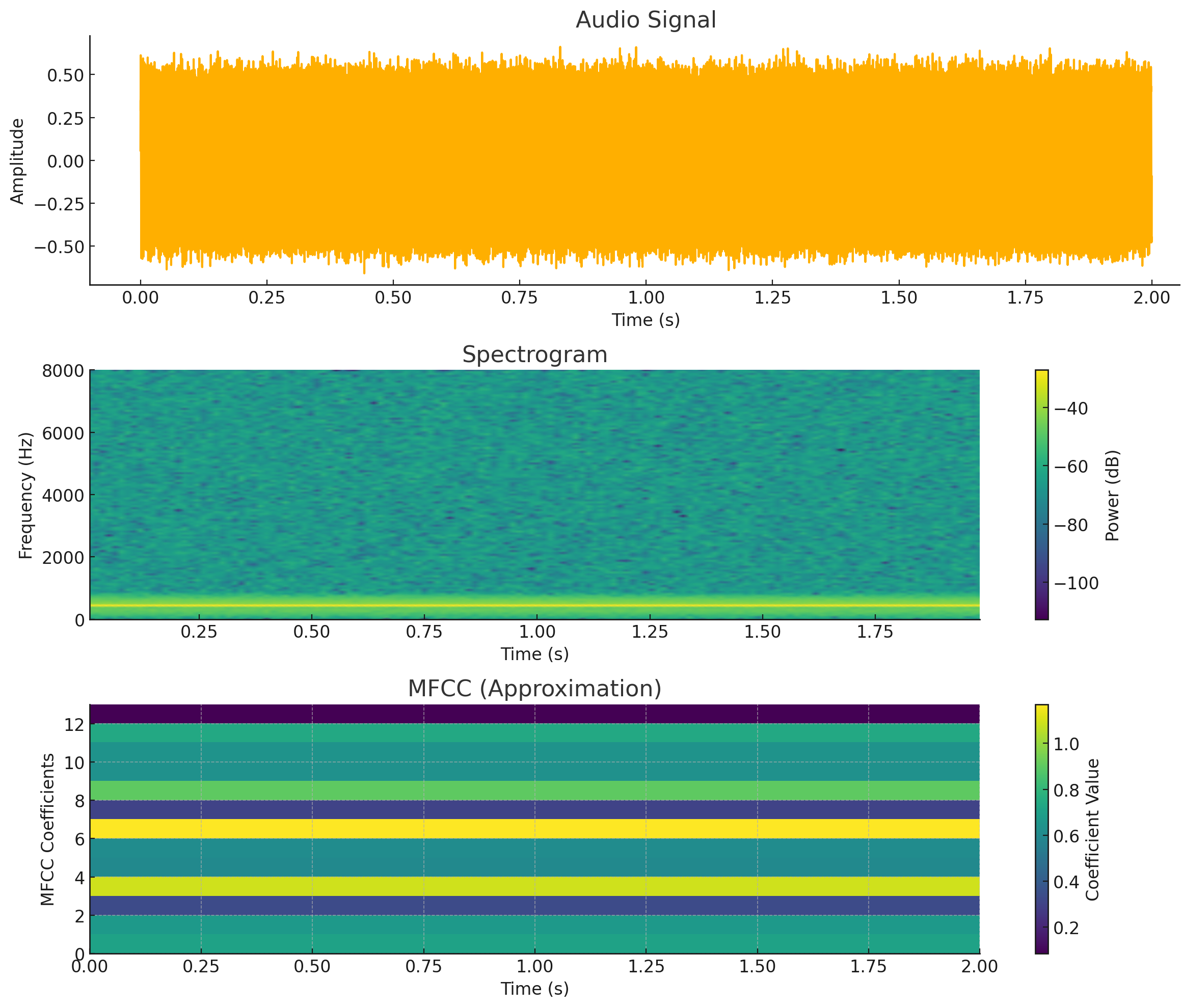
Idempotent transformations
Reliability adds retry safety to these quality foundations. While quality focuses on what transformations produce, reliability also governs how safely they can be repeated. Idempotency23 means that applying an operation repeatedly has the same effect as applying it once. This property proves essential for production ML systems where processing may be retried after failures, data may be reprocessed to fix bugs, or the same data may flow through multiple processing paths. Determinism is a related but distinct requirement: identical inputs and captured state should produce identical outputs.
23 Idempotency: From Latin idem (“the same”) + potens (“having power”) – literally, “having the same power when applied again.” In ML pipelines, idempotency enables safe retries after partial failures: a nonidempotent operation (for example, appending to a log) creates duplicates on retry. An idempotent operation leaves the same resulting state after one application or repeated applications.
Consider a light switch to build intuition. Flipping the switch to the “on” position turns the light on. Flipping it to “on” again leaves the light on; the operation can be repeated without changing the outcome. This is idempotent behavior. In contrast, a toggle switch that changes state with each press is not idempotent: pressing it repeatedly alternates between on and off states. In data processing, we want light switch behavior where reapplying the same transformation yields the same result, not toggle switch behavior where repeated application changes the outcome unpredictably.
Idempotent transformations enable reliable error recovery. When a processing job fails midway, the system can safely retry processing the same data without worrying about duplicate transformations or inconsistent state. A nonidempotent transformation might append data to existing records, so retrying would create duplicates. An idempotent transformation would upsert data (insert if not exists, update if exists), so retrying produces the same final state. This distinction becomes critical in distributed systems where partial failures are common and retries are the primary recovery mechanism.
Handling partial processing failures requires careful state management. Processing pipelines should be designed so that each stage can be retried independently without affecting other stages. Checkpoint-restart mechanisms enable recovery from the last successful processing state rather than restarting from scratch. For long-running data processing jobs operating on terabyte-scale datasets, checkpointing progress every few minutes means a failure near the end requires reprocessing only recent data rather than the entire dataset. The checkpoint logic must carefully track what data has been processed and what remains, ensuring no data is lost or processed twice.
Deterministic transformations are those that always produce the same output for the same input, without dependence on external factors like time, random numbers, or mutable global state. Transformations that depend on current time (for example, computing “days since event” based on current date) break determinism because reprocessing historical data would produce different results. The solution is to capture temporal reference points explicitly: instead of “days since event,” compute “days from event to reference date” where reference date is fixed and persisted. Random operations should use seeded random number generators where the seed is derived deterministically from input data, ensuring reproducibility.
Reliability in the KWS pipeline requires reproducible feature extraction. Audio preprocessing must be deterministic: given the same raw audio file, the same MFCC features are always computed regardless of when processing occurs or which server executes it. This enables debugging model behavior (can always recreate exact features for a problematic example), reprocessing data when bugs are fixed (produces consistent results), and distributed processing (different workers produce identical features from the same input). The processing code captures all parameters (fast Fourier transform (FFT) window size, hop length, number of MFCC coefficients) in configuration versioned alongside the code, ensuring reproducibility across time and execution environments. Even with rigorous design, production systems must implement runtime monitoring to detect skew if it emerges; ML Operations covers operational comparison and distribution monitoring at scale.
Distributed processing
Scale becomes the next constraint once quality and reliability are in place. Quality ensures transformations produce correct outputs; reliability ensures they produce consistent outputs. Neither matters if processing cannot keep pace with data volume or its deadline. As datasets and experiment concurrency grow, data processing can outgrow one machine even when the raw bytes still fit on local storage. The cleaning techniques that work on gigabytes in memory must then become partition-aware, out-of-core, or distributed without changing their semantics.
These challenges manifest when quality assessment must keep pace with incoming data, when feature engineering requires computing statistics across entire datasets before transforming individual records, and when transformation pipelines create bottlenecks at massive volumes. Processing must scale from development (gigabytes on laptops) through production (terabytes across clusters) while maintaining consistent behavior.
To address these scaling bottlenecks, data must be partitioned across multiple computing resources, which introduces coordination challenges. Distributed coordination is constrained by network round-trip times: local operations complete in microseconds while network coordination requires milliseconds, creating a 1,000\(\times\) latency difference. This constraint explains why operations requiring global coordination (like computing normalization statistics across 100 machines) create bottlenecks. Each partition computes local statistics quickly, but combining them requires information from all partitions.
Data locality becomes critical at this scale. At 10 GB/s peak throughput, transferring one terabyte of training data across a network takes on the order of 100 seconds; reading the same amount from a 5 GB/s SSD takes on the order of 200 seconds. These are the same order of magnitude, which drives ML system design toward compute-follows-data architectures.24 When processing nodes access local data at RAM speeds (50–200 GB/s) but must coordinate over networks limited to 1–10 GB/s, the bandwidth mismatch creates severe bottlenecks. Geographic distribution amplifies these challenges: cross-data center coordination must handle network latency (50–200 ms between regions), partial failures, and regulatory constraints preventing data from crossing borders. Understanding which operations parallelize easily vs. those requiring expensive coordination determines system architecture and performance characteristics. This overhead constitutes a coordination tax that limits distributed data processing. The size of this tax, and whether centralizing or aggregating is faster, depends on the ratio between network round-trip and local compute time—derived in napkin math 1.7.
24 MapReduce: Designed by Dean and Ghemawat (2004) at Google to process the company’s multi-petabyte web index across thousands of commodity machines. Its scheduler preferentially assigns map tasks to nodes that hold the input data, reducing input-network traffic. This locality-aware pattern influenced Hadoop and later distributed data-processing systems.
Dean, Jeffrey, and Sanjay Ghemawat. 2004. “MapReduce: Simplified Data Processing on Large Clusters.” Proceedings of the 6th Symposium on Operating Systems Design and Implementation (OSDI), 137–50.

Local aggregation beats gather-all when network latency dominates.
25 Parquet: A columnar storage format that organizes data by column, not by row. For the single-machine optimizations described, this is critical; instead of wastefully reading an entire CSV row to access a few columns, a Parquet reader loads only the specific columns needed for a computation. The resulting I/O reduction depends on the selected columns, encoding, compression, and workload.
Single-machine processing suffices for surprisingly large workloads when engineered carefully. Modern servers with 256 gigabytes RAM can process datasets of several terabytes using out-of-core processing that streams data from disk. Libraries like Dask or Vaex enable pandas-like APIs that automatically stream and parallelize computations across multiple cores. Before investing in distributed processing infrastructure, teams should exhaust single-machine optimization: using efficient data formats (Parquet25 instead of CSV), minimizing memory allocations, using vectorized operations, and exploiting multi-core parallelism. The operational simplicity of single-machine processing (no network coordination, no partial failures, simple debugging) makes it preferable when performance is adequate.
Napkin Math 1.7: The coordination tax
Problem: Mean normalization must be computed across 1 TB of features distributed across 100 nodes. Is it faster to (A) gather all data to one node and compute centrally, or (B) compute local means and aggregate them?
Option A (centralized):
- Transfer 1 TB at 10 GB/s network: 100 seconds
- Compute mean on single node: ~5–20 seconds at RAM bandwidth
- Total: ~105–120 seconds
Option B (distributed):
- Each node computes local mean: ~0.05–0.2 seconds (10 GB at RAM speed)
- Send 100 partial means (8 bytes each): \(<1\text{ ms}\)
- Aggregate: negligible
- Total: ~0.05–0.2 seconds (hundreds to a few thousand times faster)
Systems insight: Algebraically decomposable reductions can often use partial aggregation near the data; for example, a distributed mean carries partial sums and counts. Joins and cross-products may require shuffling, although partitioning and colocation can reduce that cost. Pipeline design should minimize unnecessary movement by pushing suitable computation toward the data, the compute-follows-data principle central to systems like MapReduce (Dean and Ghemawat 2004), Spark (Zaharia et al. 2010), and modern ML frameworks.
Zaharia, Matei, Mosharaf Chowdhury, Michael J. Franklin, Scott Shenker, and Ion Stoica. 2010. “Spark: Cluster Computing with Working Sets.” HotCloud 10: 10–10.
26 Amdahl’s law: Amdahl (1967) presented the serial-fraction argument at the 1967 AFIPS Spring Joint Computer Conference to explain why multiprocessor designs face diminishing returns. The original point – that the serial fraction of a workload imposes a hard ceiling on parallelism – applies directly to data pipelines: operations like computing global normalization statistics force serial aggregation phases that cap speedup regardless of how many workers process individual records in parallel.
Amdahl, Gene M. 1967. “Validity of the Single Processor Approach to Achieving Large Scale Computing Capabilities.” Proceedings of the April 18-20, 1967, Spring Joint Computer Conference on - AFIPS ’67 (Spring), AFIPS ’67 (spring), 483–85. https://doi.org/10.1145/1465482.1465560.
Parallelizing data ingestion across distributed workers yields diminishing throughput returns whenever unpartitionable bottlenecks—such as sequential decompression or central database lock acquisition—limit concurrency. Amdahl’s Law26 formalizes this scaling ceiling in equation 4:
\[\text{Speedup} \leq \frac{1}{f_{\text{serial}} + \frac{f_{\text{parallel}}}{N_{\text{workers}}}} \tag{4}\] where \(f_{\text{serial}}\) denotes the execution fraction spent in inherently sequential stages, \(f_{\text{parallel}}\) represents the parallelizable fraction (\(f_{\text{serial}} + f_{\text{parallel}} = 1\)), and \(N_{\text{workers}}\) denotes active worker processes. Even when 90 percent of a feature extraction pipeline parallelizes across hundreds of nodes (\(f_{\text{serial}} = 0.10\)), the maximum theoretical speedup cannot exceed \(10\times\), demonstrating why eliminating serial I/O bottlenecks takes precedence over adding compute nodes.
Framework choice follows the same coordination question as the Amdahl analysis: it depends on which parts of the transformation can run independently and which parts need shared state or ordering. Apache Spark parallelizes transformations across clusters of machines, handling data partitioning, task scheduling, and fault tolerance automatically. Beam provides a unified API for both batch and streaming processing, enabling the same transformation logic to run on multiple execution engines (Spark, Flink, Dataflow). TensorFlow’s tf.data API optimizes data loading pipelines for ML training, supporting distributed reading, prefetching, and transformation. The choice depends on whether processing is batch or streaming, how transformations parallelize, and what execution environment is available.
The feature computation placement trade-off introduced in section 1.4.5.3 takes on additional significance at scale. When distributed processing increases throughput, the cost of recomputing features across hundreds of workers per epoch must be weighed against the storage cost of materializing those features once. At terabyte scale, even small per-example compute costs multiply into significant overhead, reinforcing why production systems adopt hybrid patterns: precomputing expensive, stable features while computing cheap, time-sensitive features on-the-fly.
Scalability in the KWS pipeline manifests at multiple stages. Development uses single-machine processing on sample datasets to iterate rapidly. Training at scale may require distributed processing when the dataset (23.4 million examples) exceeds a machine’s practical capacity or when experiments run concurrently. Per-file feature extraction is embarrassingly parallel, but end-to-end speedup is bounded by shared storage bandwidth, metadata operations, scheduling, and output contention. Production deployment adds a stricter 16 KB preprocessing-state budget alongside the 64 KB model-size limit, necessitating careful footprint optimization to fit processing within device capabilities.
Transformation lineage
Governance completes the four-pillar view of data processing by ensuring accountability and reproducibility. The governance pillar requires tracking what transformations were applied, when they executed, which version of processing code ran, and what parameters were used. This transformation lineage27 supports reproducibility, debugging, auditability, and iterative improvement when transformation bugs are discovered. It can supply evidence for documentation or compliance workflows, but lineage alone does not explain a model’s decision or establish regulatory compliance.
27 Data lineage: When a model produces an erroneous or discriminatory prediction, lineage helps engineers determine whether the contributing problem originated in raw data, feature computation, training, or serving. The resulting trace can support incident investigation and jurisdiction-specific documentation duties, but its usefulness depends on complete instrumentation and retained history; it does not guarantee an explanation of model behavior.
Transformation versioning captures which version of processing code produced each dataset. When transformation logic changes (fixing a bug, adding features, or improving quality), the version number increments. Datasets are tagged with the transformation version that created them, enabling identification of all data requiring reprocessing when bugs are fixed. This versioning extends beyond just code versions to capture the entire processing environment: library versions (different NumPy versions may produce slightly different numerical results), runtime configurations (environment variables affecting behavior), and execution infrastructure (CPU architecture affecting floating-point precision).
Parameter tracking maintains the specific values used during transformation. For normalization, this means storing the mean and standard deviation computed on training data. For categorical encoding, this means storing the vocabulary (set of all observed categories). For feature engineering, this means storing any constants, thresholds, or parameters used in feature computation. These parameters are typically serialized alongside model artifacts, ensuring serving uses identical parameters to training. Modern ML frameworks like TensorFlow and PyTorch provide mechanisms for bundling preprocessing parameters with models, simplifying deployment and ensuring consistency.
Processing lineage for reproducibility tracks the complete transformation history from raw data to final features. This includes which raw data files were read, what transformations were applied in what order, what parameters were used, and when processing occurred. Lineage systems like Apache Atlas, Amundsen, or commercial offerings instrument pipelines to automatically capture this flow. When model predictions prove incorrect, engineers can trace back through lineage to identify the training data that contributed to the behavior, the quality scores attached to that data, the transformations applied, and whether the exact scenario can be recreated for investigation.
Code version ties processing results to the exact code that produced them. When processing code lives in version control (Git), each dataset should record the commit hash of the code that created it. This enables recreating the exact processing environment: checking out the specific code version, installing dependencies listed at that version, and running processing with identical parameters. Container technologies like Docker simplify this by capturing the entire processing environment (code, dependencies, system libraries) in an immutable image that can be rerun months or years later with identical results.
The governance pillar in the KWS pipeline tracks audio processing parameters that critically affect model behavior. When audio is normalized to standard volume, the reference volume level is persisted. When FFT transforms audio to frequency domain, the window size, hop length, and window function (Hamming, Hanning, etc.) are recorded. When MFCCs are computed, the number of coefficients, frequency range, and mel filterbank parameters are captured. This comprehensive parameter tracking enables several critical capabilities: reproducing training data exactly when debugging model failures, validating that serving uses identical preprocessing to training, and systematically studying how preprocessing choices affect model accuracy. Without this governance infrastructure, teams resort to manual documentation that inevitably becomes outdated or incorrect, leading to subtle training-serving skew that degrades production performance.
Clean, normalized, feature-ready data is still inert without meaning. That boundary matters operationally because a transformation can be perfectly reproducible yet attach the wrong target, and pipeline determinism cannot repair a mislabeled example. The remaining question is how to assign meaning: labels declare which audio clips contain the wake word and which are background noise, introducing human judgment into what has been an automated pipeline.
Self-Check: Question
An engineer normalizes a numerical feature by computing standard \(z\)-scores: \(x' = (x - \mu)/\sigma\). During production serving, how must the parameters \(\mu\) and \(\sigma\) be handled to satisfy the Consistency Imperative and prevent training-serving skew?
- Persist the exact \(\mu\) and \(\sigma\) computed on the training dataset alongside the model artifact, loading and applying those fixed constants to live serving inputs.
- Recompute \(\mu\) and \(\sigma\) dynamically over each incoming serving batch to ensure the live data is always centered at zero.
- Discard \(\mu\) and \(\sigma\) entirely at inference time and rely on batch normalization layers inside the neural network.
- Compute \(\mu\) and \(\sigma\) independently over a rolling 1-hour window of serving traffic to track seasonal shifts.
A distributed preprocessing job must compute global mean normalization across \(1\text{ TB}\) of feature data distributed evenly over 100 worker nodes. Architecture 1 gathers all \(1\text{ TB}\) of raw data to a central coordinator node over a \(1\text{ Gbps}\) network to compute the global mean. Architecture 2 computes a local sum and record count on each node (transferring only 16 bytes per node to the coordinator) and calculates the exact global mean locally. What is the systems trade-off and coordination tax difference?
- Centralized gathering is faster because centralizing all data eliminates worker-level floating-point rounding errors.
- Local aggregation produces only an approximation of the mean, whereas centralized gathering computes the true mathematical value.
- Both approaches take identical execution time because the total number of arithmetic additions is preserved.
- Centralized gathering incurs a massive coordination tax, taking ~8,000 seconds to transfer 1 TB over 1 Gbps, whereas local aggregation transfers under 2 KB of aggregated statistics in sub-seconds while computing the exact same mathematical mean.
Define idempotency in the context of data transformation pipelines and explain why idempotent operations (such as upserts) are essential for fault recovery in distributed ML pipelines.
True or False: Using the identical Python preprocessing function in both training and serving code repositories is sufficient to eliminate training-serving skew.
Arrange the sequential signal processing stages used in Keyword Spotting (KWS) pipelines to extract Mel-Frequency Cepstral Coefficients (MFCCs) from raw audio waveforms:
- Mel-filterbank application (emphasizing human speech frequency bands)
- Discrete Cosine Transform (DCT) for decorrelation and dimensionality reduction
- Short-Time Fourier Transform (STFT) to produce time-frequency power spectrum
- Raw audio framing and windowing (e.g., 25 ms frames)
- Pre-emphasis filtering to amplify high frequencies
Data Labeling
The processing pipelines in section 1.5 transform raw data into structured features, but supervised learning still requires labels that tell the model which patterns correspond to each target. Consider our KWS system: the ingestion and processing stages have produced millions of clean, standardized audio spectrograms, but training requires someone, or something, to declare which contain the wake word and which are background noise. This declaration is the ground truth,28 and producing it at scale is often the most human-dependent and error-prone stage of the pipeline.
28 Ground truth: From remote sensing, where orbital measurements are verified by sending a team to the physical location – the “ground” – to establish the “truth.” The etymology carries a systems warning: ML labels are proxies for reality, not reality itself. When a crowdsourced annotator labels an image as “cat,” that label reflects the annotator’s judgment, not an objective fact. Every downstream metric – accuracy, precision, recall – is measured against this proxy, meaning label quality errors propagate silently into every evaluation of the model.
Unlike automated transformations that can be parallelized across machines, labeling introduces human judgment into the pipeline, creating unique engineering challenges. A crowdsourced annotator might mislabel a whispered “Alexa” as background noise. An expert radiologist might disagree with a colleague about a borderline diagnosis. Such disagreement can reflect genuine ambiguity, unclear instructions, annotator error, or differences in expertise; the labeling system must distinguish and manage these causes rather than treating every disagreement as irreducible. The infrastructure must therefore handle throughput, quality control, cost management, and governance.
Label types and system requirements
Building effective labeling systems requires understanding how different label types affect system architecture and resource requirements. Consider a practical example: building a smart city system that needs to detect and track various objects like vehicles, pedestrians, and traffic signs from video feeds. Labels capture information about key tasks or concepts, with each label type imposing distinct storage, computation, and validation requirements.
Classification labels represent the simplest form, categorizing images with a specific tag or (in multi-label classification) tags such as labeling an image as “car” or “pedestrian.” While conceptually straightforward, a production system processing millions of video frames must efficiently store and retrieve these labels. Storage requirements are modest (a single integer or string per image), but retrieval patterns matter: training often samples random subsets while validation requires sequential access to all labels, driving different indexing strategies.
Bounding boxes extend beyond simple classification by identifying object locations, drawing a box around each object of interest. Our system must track both object identity and spatial location within each frame. This spatial information introduces new storage and processing challenges, especially when tracking moving objects across video frames. Each bounding box stores four coordinates (x, y, width, height) plus the object class, so storage scales with the number of annotated objects per image rather than a fixed-size label per image. Bounding box annotation requires pixel-precise positioning that takes 10–20\(\times\) longer than classification, dramatically affecting labeling throughput and cost.

Finer annotation granularity multiplies storage and processing scale.
Segmentation maps provide the most comprehensive information by classifying objects at the pixel level, highlighting each object in a distinct color. For our traffic monitoring system, this might mean precisely outlining each vehicle, pedestrian, and road sign. These detailed annotations significantly increase our storage and processing requirements. A segmentation mask for a \(1920{\times}1080\) image requires about 2.1M labels (one per pixel), compared to perhaps 10 bounding boxes or a single classification label. If each box stores 4 coordinates, that is roughly 51,840× more scalar label entries than 10 boxes before accounting for per-value encoding, and the hours required per image for manual segmentation make this approach suitable only when pixel-level precision is essential.
Figure 11 contrasts five annotation modalities, and the choice depends on the input, task, and available annotation budget. Classification can label an entire scene, while bounding boxes and segmentation maps localize objects or regions. Production datasets may combine modalities: a single camera frame might carry a scene label, obstacle boxes, and path-region masks, with each label type serving a distinct downstream task.
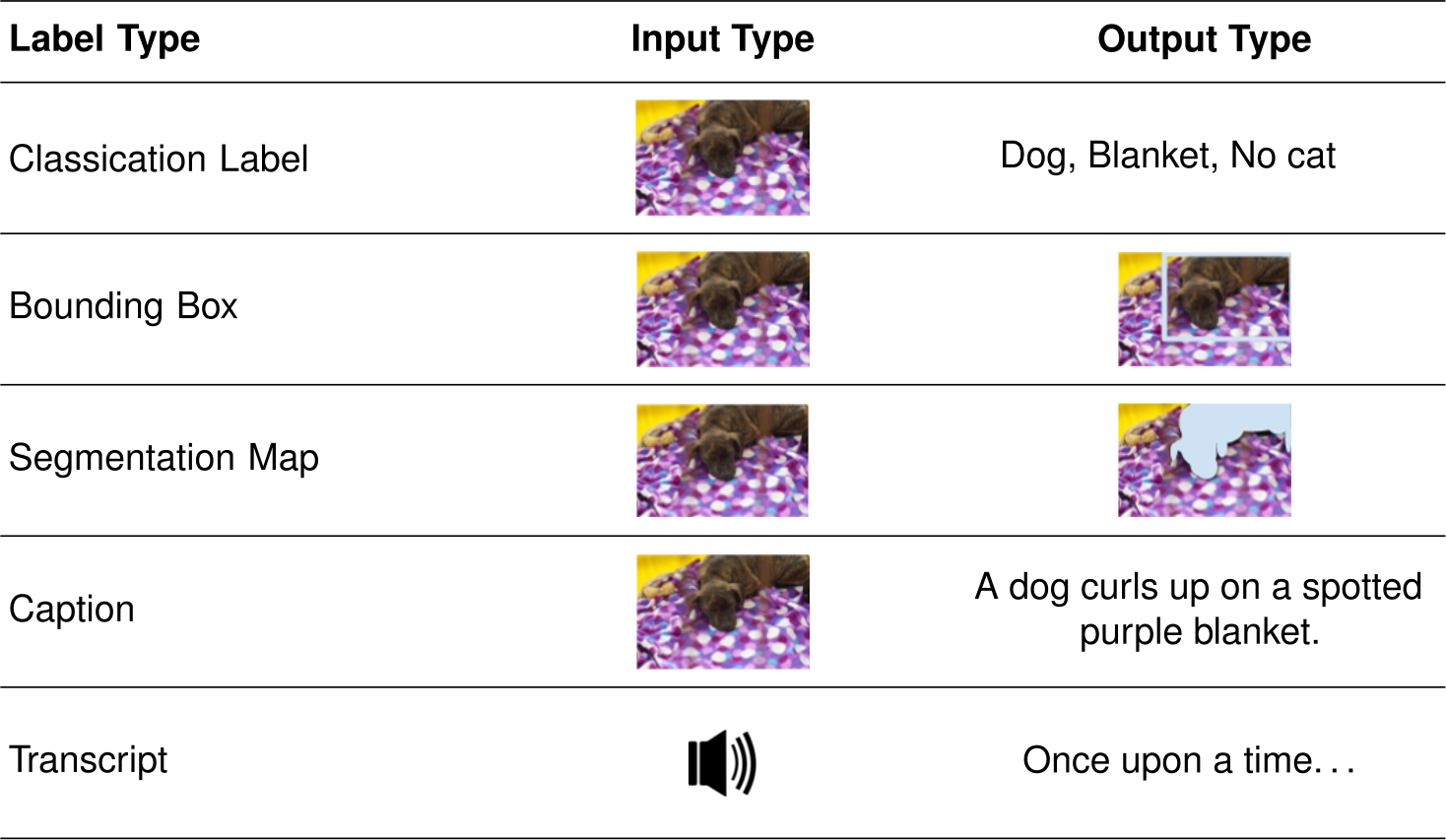
Beyond these geometric labels, production systems must also manage rich metadata essential for quality control and debugging. The Common Voice dataset (Ardila et al. 2020) exemplifies this in speech recognition: tracking speaker demographics for fairness, recording quality metrics for filtering, and language information for multilingual support. If our traffic monitoring system fails in rainy conditions, weather metadata captured during collection pinpoints the coverage gap. This metadata requirement demonstrates how label type choice cascades through entire system design: the infrastructure must optimize storage for the chosen format, implement appropriate retrieval patterns, and track which model versions used which label versions to correlate quality improvements with performance gains.
Ardila, Rosana, Megan Branson, Kelly Davis, Michael Kohler, Josh Meyer, Michael Henretty, Reuben Morais, Lindsay Saunders, Francis Tyers, and Gregor Weber. 2020. “Common Voice: A Massively-Multilingual Speech Corpus.” Proceedings of the Twelfth Language Resources and Evaluation Conference, 4218–22.
Label accuracy and consensus
In the labeling domain, label quality centers on ensuring label accuracy despite the inherent subjectivity and ambiguity in many labeling tasks. Even with clear guidelines and careful system design, some fraction of labels will inevitably be incorrect (Northcutt et al. 2021; Thyagarajan et al. 2022). The challenge is not eliminating labeling errors entirely (an impossible goal) but systematically measuring inter-annotator agreement and managing error rates to keep them within bounds that do not degrade model performance.
Thyagarajan, Aditya, Elı́as Snorrason, Curtis G. Northcutt, and Jonas Mueller. 2022. “Identifying Incorrect Annotations in Multi-Label Classification Data.” CoRR abs/2211.13895. https://doi.org/10.48550/ARXIV.2211.13895.
Labeling failures arise from two distinct sources requiring different engineering responses. Figure 12 presents concrete examples of both failure modes. Some examples reflect degraded or ambiguous inputs where the correct label is difficult to infer from the data alone; others are visually clear but require domain knowledge, dataset-specific semantics, or expert judgment to label correctly. These different failure modes drive architectural decisions about annotator qualification, task routing, and consensus mechanisms: quality-based errors call for upstream data filtering, while expertise-based errors call for tiered annotator routing.
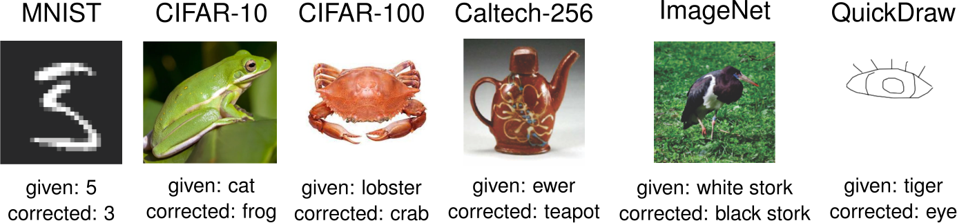
Northcutt, Curtis G., Anish Athalye, and Jonas Mueller. 2021. “Pervasive Label Errors in Test Sets Destabilize Machine Learning Benchmarks.” arXiv Preprint arXiv:2103.14749 34: 19075–90. https://doi.org/10.48550/arxiv.2103.14749.
Given these inherent quality challenges, production ML systems implement multiple layers of quality control. Systematic quality checks continuously monitor the labeling pipeline through random sampling of labeled data for expert review and statistical methods to flag potential errors. The infrastructure must efficiently process these checks across millions of examples without creating bottlenecks. Sampling strategies typically validate 1-10 percent of labels, balancing detection sensitivity against review costs. Higher-risk applications like medical diagnosis or autonomous vehicles may validate 100 percent of labels through multiple independent reviews, while lower-stakes applications like product recommendations may validate only 1 percent through spot checks.
Beyond random sampling approaches, collecting multiple labels per data point, often referred to as “consensus labeling,” can help identify controversial or ambiguous cases. Commercial labeling platforms such as Labelbox and Scale AI expose consensus and tiered quality-control workflows (Labelbox, Inc. 2024; Scale AI, Inc. 2024), but the statistical core is inter-annotator agreement. The consensus infrastructure typically collects several labels per example, computing metrics like Fleiss’ kappa, a generalization of the Cohen’s kappa statistic introduced in section 1.4.3 from two raters to any number of annotators (Fleiss 1971). Examples with low agreement, using thresholds such as the Landis-Koch bands as operational heuristics, route to expert review rather than forcing consensus from genuinely ambiguous cases (Landis and Koch 1977).
Labelbox, Inc. 2024. Labelbox Consensus Documentation.
Scale AI, Inc. 2024. Scale AI Advanced Settings.
Fleiss, Joseph L. 1971. “Measuring Nominal Scale Agreement Among Many Raters.” Psychological Bulletin 76 (5): 378–82. https://doi.org/10.1037/h0031619.
The consensus approach reflects an economic trade-off essential for scalable systems. Expert review costs more per example than crowdsourced labeling, but forcing agreement on ambiguous examples through majority voting of nonexperts can produce systematically biased labels. By routing only genuinely ambiguous cases to experts, identified through low inter-annotator agreement or failed gold-standard checks, systems balance cost against quality. This tiered approach enables processing millions of examples economically while maintaining quality standards through targeted expert intervention.
While technical infrastructure provides the foundation for quality control, successful labeling systems must also consider human factors. When working with annotators, organizations need reliable systems for training and guidance. This includes good documentation with clear examples of correct labeling, visual demonstrations of edge cases and how to handle them, regular feedback mechanisms showing annotators their accuracy on gold standard examples, and calibration sessions where annotators discuss ambiguous cases to develop shared understanding. For complex or domain-specific tasks, the system might implement tiered access levels, routing challenging cases to annotators with appropriate expertise based on their demonstrated accuracy on similar examples.
Quality monitoring generates substantial data that must be efficiently processed and tracked. The most informative signals span several dimensions. Inter-annotator agreement rates reveal whether multiple annotators converge on the same example, while label confidence scores capture how certain annotators feel about their decisions. Time per annotation serves as a dual-sided indicator: annotations completed too quickly suggest carelessness, while those taking too long suggest confusion or unclear guidelines. Error patterns expose systematic biases or misunderstandings in the annotator pool, and annotator performance on gold standard examples provides ground-truth calibration. Finally, demographic analysis of annotator behavior detects whether certain groups systematically label differently, which could introduce unintended bias into the training data. These metrics must be computed and updated efficiently across millions of examples, often requiring dedicated analytics pipelines that process labeling data in near real-time to catch quality issues before they affect large volumes of data.
Scaling with AI-assisted labeling
The scalability pillar drives AI assistance as a force multiplier for human labeling rather than a replacement. Manual annotation alone may not keep pace with a system’s data needs, while fully automated labeling cannot supply reliable judgment for every ambiguous or high-stakes case. AI-assisted labeling occupies the space between these extremes: using automation to handle clear cases and accelerate annotation while preserving human review where it matters. Figure 13 maps four common paths. Traditional supervision uses direct human labels. Semi-supervised learning exploits structure in unlabeled data alongside a labeled subset. Weak supervision replaces some individual annotations with programmatic labeling functions. Transfer learning reuses representations learned on another task, often reducing but not eliminating task-specific labels. Each path changes where supervision cost is paid and which assumptions, unlabeled-data structure, or pretrained artifacts the pipeline must validate.
\begin{tikzpicture}[font=\small\sffamily]
%
\tikzset{%
  Line/.style={line width=1.0pt,black!50,text=black},
  Box/.style={align=flush center,
   inner sep=5pt,
    node distance=0.75,
    draw=GreenLine,
    line width=0.75pt,
    fill=GreenL,
    text width=55mm,
    minimum width=53mm, minimum height=9mm
  },
   Box1/.style={Box,
    node distance=0.35,
    draw=OrangeLine,
    line width=0.75pt,
    fill=OrangeL,
    text width=31mm,
    minimum width=31mm, minimum height=8.2mm
  },
  Box2/.style={Box,
    node distance=0.5,
    draw=BlueLine,
    line width=0.75pt,
    fill=BlueL,
    text width=42mm,
    minimum width=42mm, minimum height=9mm
  },
 Text/.style={%
    inner sep=2pt,
    draw=none,
    line width=0.75pt,
    fill=TextColor,
    text=black,
    font=\footnotesize\sffamily,
    align=flush center,
    minimum width=7mm, minimum height=5mm
  },
}
%
\node[Box,text width=65mm,minimum width=62mm, minimum height=10mm,
           fill=RedL,draw=RedLine](B1){\textbf{How to get more labeled training data?}};
\node[Box, node distance=0.5,below=of B1,xshift=12mm](B2){\textbf{Traditional Supervision:} Have subject
              matter experts (SMEs) hand-label more training data};
\node[Box,below=0.3 of B2](B3){\textbf{Semi-supervised Learning:} Use structural
            assumptions to automatically use unlabeled data};
\node[Box,below=0.3 of B3](B4){\textbf{Weak Supervision:}\\ Get lower-quality
            labels more efficiently and/or at a higher abstraction level};
\node[Box,below=0.3 of B4](B5){\textbf{Transfer Learning:}\\ Use models
            already trained on a different task};
%
\node[Box2,above right=0.7 and 1.75 of B2,fill=BrownL,draw=BrownLine](2B1){Too expensive!};
\node[Box2,below =0.15 of 2B1,fill=BrownL,draw=BrownLine](2B2){\textbf{Active Learning:} Estimate
            which points are most valuable to solicit labels for};
%
\node[Box2,above right=1.05 and 1.75 of B4](2B3){Get cheaper, lower-quality labels from nonexperts};
\node[Box2,below =0.2 of 2B3](2B4){Get higher-level supervision
            over unlabeled data from SMEs};
\node[Box2,below =0.2 of 2B4](2B5){Use one or more
              (noisy/biased) pretrained models to provide supervision};
%
\node[Box1,above right=0.25 and 1.45 of 2B3](3B1){Heuristics};
\node[Box1,below =of 3B1](3B2){Distant Supervision};
\node[Box1,below =of 3B2](3B3){Constraints};
\node[Box1,below =of 3B3](3B4){Expected distributions};
\node[Box1,below =of 3B4](3B5){Invariances};
%%
\foreach \x in{2,3,4,5}{
\draw[-latex,Line](B1.191)|-(B\x);
}

\foreach \x in{1,2}{
\draw[-latex,Line](B2.east)--++(0:1.1)|-(2B\x);
}

\foreach \x in{3,4,5}{
\draw[-latex,Line](B4.355)--++(0:1.1)|-(2B\x);
}

\foreach \x in{1,2,3,4,5}{
\draw[-latex,Line](2B4.east)--++(0:0.8)|-(3B\x);
}
\draw[-latex,Line](2B2)--++(270:1.0)--++(180:3.5)|-(B4.05);
\draw[-latex,Line](B5.355)-|(2B5);
\end{tikzpicture}
Ratner, Alex, Paroma Varma, Braden Hancock, and Christopher Ré. 2019. Weak Supervision: A New Programming Paradigm for Machine Learning. Stanford AI Lab Blog.
These paths exchange different assumptions, not just label counts. Depending on the path, the pipeline needs task-relevant structure in unlabeled data, a transferable representation, measurable labeling-function errors, or an affordable scoring loop. Production systems should record each assumption and test it against held-out, human-reviewed data. The diagram is a decision map, not a quality ranking.
AI-assisted labeling divides work according to the strengths of each participant. Humans judge ambiguous cases, catch subtle errors, and apply domain knowledge; models can process routine cases at scale, subject to validation. Production systems combine these capabilities through several complementary approaches.
Pre-annotation uses AI models to generate preliminary labels that humans then review and correct – transforming the task from “label from scratch” to “verify and fix.” Programmatic labeling frameworks like Snorkel (Ratner et al. 2018; Ratner et al. 2017) extend this further through weak supervision,29 automatically generating initial labels at scale through rule-based heuristics, knowledge bases, and existing model outputs. In autonomous driving, pretrained object detection models can label vehicles and pedestrians that human annotators verify and refine, handling many clear cases automatically.
Ratner, Alex, Braden Hancock, Jared Dunnmon, Roger Goldman, and Christopher Ré. 2018. “Snorkel MeTaL: Weak Supervision for Multi-Task Learning.” Proceedings of the Second Workshop on Data Management for End-to-End Machine Learning, 1–4. https://doi.org/10.1145/3209889.3209898.
Ratner, A., S. H. Bach, H. Ehrenberg, J. Fries, S. Wu, and C. Ré. 2017. “Snorkel: Rapid Training Data Creation with Weak Supervision.” Proceedings of the VLDB Endowment 11 (3): 269–82. https://doi.org/10.14778/3157794.3157797.
29 Weak supervision: A “data programming” paradigm that exchanges some manual annotation labor for the upfront effort of writing and validating programmatic labeling functions. Once written, a function can be applied cheaply at scale, but execution, conflict resolution, quality monitoring, and maintenance still incur cost; the useful comparison is workload-specific rather than literally zero marginal cost.
Large language models (LLMs) now assist labeling pipelines by generating descriptions, drafting labeling guidelines from examples, and explaining their reasoning for label assignments. Content moderation systems, for instance, use LLMs for initial content classification with explanations that human reviewers validate. However, LLM integration introduces systems challenges: provider- and model-dependent inference costs and rate limits, as well as the need for systematic output validation because LLMs can produce confident but incorrect labels. Many organizations adopt tiered approaches, using smaller specialized models for routine cases while reserving larger LLMs for complex scenarios requiring nuanced judgment.
Active learning makes the complementary trade-off: it spends model inference to reduce human labeling, so the relevant question is whether that compute fits inside the same budget.
Methods such as active learning30 complement these approaches by intelligently prioritizing which examples need human attention (Settles 2009; Coleman et al. 2022). These systems continuously analyze model uncertainty to identify valuable labeling candidates. Rather than labeling a random sample of unlabeled data, active learning selects examples where the current model is most uncertain or where labels would most improve model performance. The infrastructure must efficiently compute uncertainty metrics (often prediction entropy or disagreement between ensemble models), maintain task queues ordered by informativeness, and adapt prioritization strategies based on incoming labels. Consider a medical imaging system: active learning might identify unusual pathologies for expert review while handling routine cases through preannotation that experts merely verify. This approach can substantially reduce required annotations in favorable settings, though it requires careful engineering to prevent feedback loops where the model’s uncertainty biases which data gets labeled. A budget calculation makes that leverage concrete.
30 Active learning: Inverts the traditional labeling paradigm: instead of randomly selecting examples to label, the model queries for the examples it needs most, typically those where prediction uncertainty is highest (Settles 2009). This can reduce the number of labels needed to reach a target accuracy, but the infrastructure trade-off is compute for labels: at $0.01/image, scoring a full 10M pool costs $100K before any human labels. Active learning becomes budget leverage only when the candidate pool is pre-filtered, inference is much cheaper, or the compute budget is separate from the labeling budget.
Settles, Burr. 2009. Active Learning Literature Survey. Computer Sciences Technical Report 1648. University of Wisconsin-Madison.
Coleman, Cody, Edward Chou, Julian Katz-Samuels, Sean Culatana, Peter Bailis, Alexander C. Berg, Robert Nowak, Roshan Sumbaly, Matei Zaharia, and I. Zeki Yalniz. 2022. “Similarity Search for Efficient Active Learning and Search of Rare Concepts.” Proceedings of the AAAI Conference on Artificial Intelligence 36 (6): 6402–10. https://doi.org/10.1609/aaai.v36i6.20591.
Napkin Math 1.8: The active learning multiplier
Problem: A 10M dataset has a $50K labeling budget. Random sampling achieves 85 percent accuracy with 100K, while the target is 95 percent accuracy.
Physics:
- Sample efficiency: Active learning can achieve target accuracy with fewer samples than random selection in favorable settings.
- Cost per point: Random sampling = $0.50/label. Active learning adds compute cost (~$0.01/image for inference) to find hard examples.
- Multiplier:
- Random: Reaching 95 percent may require 1M labels ($500K). Budget exceeded.
- Active labels only: The system may need ~100K–200K hard examples ($50K–$100K).
- Full-pool scoring: Scoring all 10M candidate images adds $100K, so total active-learning cost becomes $150K–$200K. Budget exceeded.
Systems insight: Algorithm choice is a major lever on label count, but compute must be inside the budget model. Spending 10 percent of this budget on inference ($5K) scores only 500K candidate images at the stated inference price and leaves room for about 90K labels. Active learning is viable only if the candidate pool is narrowed before scoring, inference cost drops substantially, or compute is funded separately from labeling.

Full-pool scoring can exceed the label budget before labeling begins.
Quality control becomes increasingly important as these AI components interact. The system must monitor both AI and human performance through systematic metrics. Model confidence calibration matters: if the AI reports 95 percent confidence but achieves only 75 percent accuracy at that confidence level, preannotations mislead human reviewers. Human-AI agreement rates reveal whether AI assistance helps or hinders: when humans frequently override AI suggestions, the preannotations may be introducing bias rather than accelerating work. These metrics require careful instrumentation throughout the labeling pipeline, tracking both final labels and the interaction between human annotators and AI at each stage.
These principles manifest at scale across safety-critical domains. Autonomous vehicle labeling infrastructure can process large volumes of sensor frames, using AI preannotation to label common objects while routing unusual scenarios (construction zones, emergency vehicles) to human experts–a distributed architecture where preannotation runs on GPU clusters while human review scales across annotation teams. Medical imaging systems face a parallel label-scarcity problem: large repositories of unlabeled clinical data make expert annotation the bottleneck and motivate data-efficient workflows that learn useful representations from unlabeled structure before expert labels are applied (Krishnan et al. 2022). Across such domains, the common data-engineering pattern is tiered escalation: automation handles clear cases, humans handle ambiguous ones, and monitoring ensures the boundary between “clear” and “ambiguous” adapts as both AI capability and deployment conditions evolve.
Krishnan, Rayan, Pranav Rajpurkar, and Eric J. Topol. 2022. “Self-Supervised Learning in Medicine and Healthcare.” Nature Biomedical Engineering 6 (12): 1346–52. https://doi.org/10.1038/s41551-022-00914-1.
Automated labeling in KWS
Labeling our KWS data at scale creates a speech-specific challenge. Generating millions of labeled wake word samples without proportional human annotation cost requires moving beyond the manual and crowdsourced approaches introduced earlier. The Multilingual Spoken Words Corpus (MSWC) (Mazumder et al. 2021) demonstrates how automated labeling addresses this challenge through its innovative approach to generating labeled wake word data; the corpus contains over 23.4 million examples of one-second speech across 340,000 keywords in 50 languages.
Mazumder, Mark, Sharad Chitlangia, Colby Banbury, Yiping Kang, Juan Manuel Ciro, Keith Achorn, Daniel Galvez, et al. 2021. “Multilingual Spoken Words Corpus.” Advances in Neural Information Processing Systems 35 (NeurIPS 2021) Datasets and Benchmarks Track.
31 Forced alignment: Given a known transcription, an aligner estimates where its words occur in the audio, often using frame-level acoustic scores and sequence decoding. Timing resolution and accuracy depend on the model, features, language, and recording quality, so boundary estimates still need quality checks. The known transcript makes word-level segmentation far cheaper than labeling every clip manually, though computation, review, and error correction remain.
This scale makes manual annotation impractical: 23.4 million examples at even 10 seconds per label would require approximately 65,000 hours, roughly 32.5 person-years of full-time effort. Broad, documented sourcing across 50 languages can improve coverage, but language count alone does not guarantee representative speakers, accents, devices, or acoustic environments. The automated system in figure 14 addresses the scale problem by starting with paired sentence audio and transcriptions, then using forced alignment31 to estimate word boundaries within continuous speech.
At this scale, quality control becomes a sampling and provenance problem rather than disappearing. The pipeline should report coverage by language, speaker, accent, device, and acoustic environment; retain the source recording, transcript version, aligner version, and boundary confidence for each extracted clip; and route low-confidence alignments and underrepresented slices to human review. Held-out evaluation must then measure the intended wake words across those slices. These controls distinguish a large corpus from a representative one and make extraction errors traceable when a downstream KWS model fails.
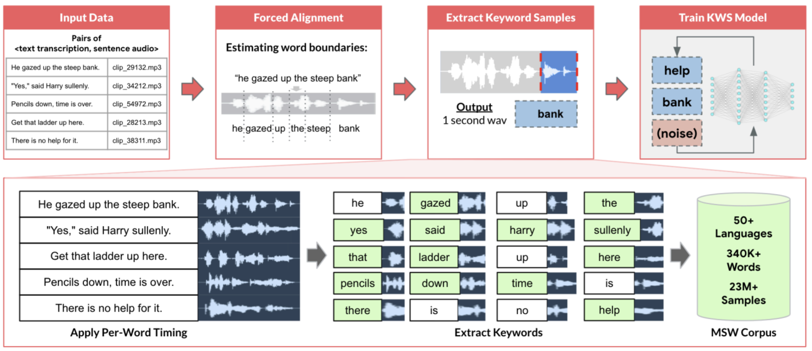
Mazumder, Mark. 2021. TinyML: Multilingual Spoken Words Corpus. tinyML Talks.
The extraction system uses these precise timing markers to generate clean keyword samples while handling the engineering challenges our problem definition anticipated: background noise interfering with word boundaries, speakers stretching or compressing words unexpectedly beyond our target 500 ms–800 ms duration, and longer words exceeding the one-second boundary. MSWC provides automated quality assessment that analyzes audio characteristics to identify potential issues with recording quality, speech clarity, or background noise, which is essential for maintaining consistent standards across 23.4 million samples without the manual review expenses that would make this scale prohibitive.
Modern voice assistant developers often build on this automated labeling foundation. While automated corpora may not contain the specific wake words a product requires, they provide starting points for KWS prototyping, particularly in underserved languages where commercial datasets do not exist. Production systems typically layer targeted human recording and verification for challenging cases (unusual accents, rare words, or difficult acoustic environments), coordinating between automated processing and human expertise.
The pipeline has now produced its compilation artifacts: millions of feature vectors paired with ground truth labels. The question shifts from what data has been collected to where it lives and how fast it reaches the accelerators. Storage architecture determines whether expensive GPUs spend their time computing or waiting.
Self-Check: Question
A smart city perception system evaluates annotation formats for a \(1920 \times 1080\) video stream. The team compares bounding box annotations (10 boxes per frame, each with 4 spatial coordinates) against pixel-level semantic segmentation masks. What is the ratio of scalar label entries generated between a full segmentation mask and the 10 bounding boxes?
- Roughly 10x more entries for segmentation, matching the ratio of bounding box coordinates.
- Roughly 50,000x more scalar entries for segmentation (~2.07 million pixel labels vs. 40 bounding box coordinates).
- Both formats require identical scalar entries because both represent 1080p resolution.
- Bounding boxes require 50,000x more entries because floating-point coordinates consume more bytes than integer masks.
An ML team implements weak supervision (e.g., using Snorkel) to label a million unlabeled text documents. Domain experts write 20 programmatic labeling functions (LFs) based on regex patterns and keyword heuristics. How does weak supervision combine these noisy heuristics into high-quality training labels?
- It forces all 20 LFs to execute synchronously in a database trigger, throwing an exception if any two LFs disagree.
- It simply computes an unweighted majority vote across all LFs and discards any record where LFs disagree.
- It uses a generative label model to estimate the unknown accuracies and correlations of the LFs without ground truth, producing probabilistic training labels for downstream model learning.
- It converts the regex heuristics into neural network weights using automatic differentiation.
Describe how a tiered consensus labeling system uses inter-annotator agreement metrics (such as Fleiss’ kappa) and ‘gold standard’ honeypot examples to balance labeling cost against annotation quality.
True or False: In Active Learning, uncertainty sampling selects the unlabeled examples for which the current model has the highest prediction confidence to ensure the training set contains only clean data.
A statistical metric that measures the degree of agreement among three or more annotators classifying items into discrete categories, adjusting for chance agreement, is called ____.
Storage Architecture
The labeled datasets from our pipeline (23.4 million samples spanning 50 languages for KWS) now require strategic storage decisions that determine training efficiency, serving latency, and long-term maintainability. Storage architecture addresses a core tension: batch training requires sequential scans across millions of examples, while real-time serving demands millisecond lookups of individual feature vectors. These competing access patterns shape every storage decision.
ML storage requirements diverge from those of transactional systems. Rather than optimizing for frequent small writes and point lookups that characterize e-commerce or banking, ML workloads prioritize high-throughput sequential reads, large-scale scans, and schema flexibility. A database serving an e-commerce application performs well with millions of individual product lookups per second, but an ML training job scanning that entire catalog repeatedly across epochs requires completely different storage optimization.
Storage system options
Batch training scans millions of examples sequentially; real-time serving fetches one feature vector at a time. These opposing access patterns pull storage in two directions, and selecting a system means minimizing the data term \((\frac{D_{\text{vol}}}{\text{BW}})\) of the iron law of ML systems for whichever pattern dominates. Every storage medium imposes physical constraints on bandwidth that determine the maximum speed of the training and serving pipelines.
Two storage performance metrics govern this optimization. IOPS (input/output operations per second) counts the distinct read/write requests a device can handle per second, so it limits random access workloads such as fetching small batches of images or individual user profiles. Throughput (bandwidth) measures the volume of data transferred per second, typically \(\text{IOPS} \times \text{Block Size}\), so it limits sequential access workloads such as scanning a Parquet file for training.
The choice between databases, data warehouses, and data lakes is fundamentally a choice about which of these metrics to optimize. Databases (online transaction processing [OLTP] systems) optimize for high IOPS with small block sizes, making them suited for serving individual feature vectors in real-time where per-request latency dominates. Data warehouses (online analytical processing [OLAP] systems) optimize for high throughput with large block sizes and sequential access, making them ideal for feature engineering and batch analytics. Data lakes prioritize capacity and throughput for unstructured data, essential for training jobs where the \(D_{\text{vol}}\) numerator is measured in petabytes and aggregate bandwidth must scale to thousands of GPUs.
The access-pattern decision becomes concrete when matched to ML workflow stages. For online feature serving, the high-IOPS characteristics of databases enable millisecond lookups of individual records. Large recommendation systems exemplify this challenge at its most extreme: terabyte-scale lookup data may need to serve billions of sparse reads per second, requiring storage architectures that optimize IOPS over sequential throughput. More generally, a recommendation system looking up a user’s profile during real-time inference requires random access optimized for per-request latency.
Structured model training points the decision in the opposite direction: throughput dominates request-level latency. The throughput-optimized design of data warehouses enables high-speed sequential scans over large, clean tables. Training a fraud detection model that processes millions of transactions with hundreds of features per transaction benefits from columnar storage that reads only relevant features efficiently, directly reducing the data term by minimizing bytes transferred.
Exploratory analysis and unstructured training data add a third constraint: the schema may not be known when the data is collected. For images, audio, and text, data lakes provide the flexibility and low-cost storage needed for massive volumes. A computer vision system storing terabytes of raw images alongside metadata, annotations, and intermediate processing results benefits from the schema flexibility and cost efficiency that data lakes commonly provide, while the scale of the \(D_{\text{vol}}\) numerator demands high aggregate bandwidth.
Databases earn their place when transactional consistency and point-lookup latency dominate. They maintain product catalogs, user profiles, or transaction histories with strong consistency guarantees and low-latency point lookups. For ML workflows, databases serve specific roles well: storing feature metadata that changes frequently, managing experiment tracking where transactional consistency matters, or maintaining model registries that require atomic updates. A PostgreSQL database handling structured user attributes (user_id, age, country, preferences) provides millisecond lookups for serving systems that need individual user features in real-time. However, databases struggle when ML training requires scanning millions of records repeatedly across multiple epochs. The row-oriented storage that optimizes transactional lookups becomes inefficient when training needs only 20 of 100 columns from each record but must read entire rows to extract those columns.
Data warehouses earn their place when repeated scans over structured features dominate. Columnar storage formats (Stonebraker et al. 2018) enable reading specific features without loading entire records, essential when tables contain hundreds of columns but training needs only a subset. The I/O reduction scales with the fraction of columns selected: reading 20 of 100 columns transfers about one fifth of the uncompressed row payload before compression or metadata overhead. The format-efficiency calculation in section 1.7.2 quantifies this gain with a worked fraud-detection example. Many successful ML systems draw training data from warehouses because the structured environment simplifies exploratory analysis and iterative development. Data analysts can quickly compute aggregate statistics, identify correlations between features, and validate data quality using familiar SQL interfaces.
Stonebraker, Mike, Daniel J. Abadi, Adam Batkin, Xuedong Chen, Mitch Cherniack, Miguel Ferreira, Edmond Lau, et al. 2018. “C-Store: A Column-Oriented DBMS.” In Making Databases Work: The Pragmatic Wisdom of Michael Stonebraker. Association for Computing Machinery. https://doi.org/10.1145/3226595.3226638.
However, warehouses assume relatively stable schemas and struggle with truly unstructured data (images, audio, free-form text) or rapidly evolving formats common in experimental ML pipelines. When a computer vision team wants to store raw images alongside extracted features, multiple annotation formats from different labeling vendors, intermediate model predictions, and learned representation vectors, forcing all these into rigid warehouse schemas creates more friction than value. Schema evolution becomes painful: adding new feature types requires ALTER TABLE operations that may take hours on large datasets, blocking other operations and slowing iteration velocity.
Data lakes earn their place when schema flexibility and low-cost retention dominate. They address warehouse limitations by storing structured, semi-structured, and unstructured data in native formats, deferring schema definitions until the point of reading, a pattern called schema-on-read.32
32 Schema-on-read: Applies data structure definitions at query time rather than during ingestion, contrasting with schema-on-write (traditional databases) where data must conform to a predefined structure before storage. For ML pipelines in early development, schema-on-read enables rapid experimentation – teams can store raw sensor data, images, and logs without committing to a feature schema upfront. The trade-off is governance: without enforced schemas, data lakes degrade into “data swamps” where finding and validating training data becomes the bottleneck instead.
This flexibility proves valuable during early ML development when teams experiment with diverse data sources and are not yet certain which features will prove useful. A recommendation system might store in the same data lake: transaction logs as JSON, product images as JPEGs, user reviews as text files, clickstream data as Parquet, and model embeddings as NumPy arrays. Rather than forcing these heterogeneous types into a common schema upfront, the data lake preserves them in their native formats. Applications impose schema only when reading, enabling different consumers to interpret the same data differently: one team extracts purchase amounts from transaction logs while another analyzes temporal patterns, each applying schemas suited to their analysis.
That flexibility is only useful if governance prevents the lake from becoming opaque. Without disciplined metadata management and cataloging, data lakes degrade into “data swamps,” disorganized repositories where finding relevant data becomes nearly impossible, undermining the productivity benefits that motivated their adoption. A data lake might contain thousands of datasets across hundreds of directories with names like userdata_v2_final and userdata_v2_final_ACTUALLY_FINAL, where only the original authors (who have since left the company) understand what distinguishes them. Successful data lake implementations maintain searchable metadata about data lineage, quality metrics, update frequencies, ownership, and access patterns, essentially providing warehouse-like discoverability over lake-scale data. Tools like AWS Glue Data Catalog, Apache Atlas, or Databricks Unity Catalog provide this metadata layer, enabling teams to discover and understand data before investing effort in processing it.
Each storage architecture favors a different access pattern and ML workflow stage, as table 7 makes explicit. A poor match can impose substantial performance penalties.
| Attribute | Conventional Database | Data Warehouse | Data Lake |
|---|---|---|---|
| Purpose | Operational and transactional | Analytical and reporting | Storage for raw and diverse data for future processing |
| Data type | Structured | Structured | Structured, semi-structured, and unstructured |
| Scale | Small to medium volumes | Medium to large volumes | Large volumes of diverse data |
| Performance Optimization | Optimized for transactional queries (OLTP) | Optimized for analytical queries (OLAP) | Optimized for scalable storage and retrieval |
| Examples | MySQL, PostgreSQL, Oracle DB | Google BigQuery, Amazon Redshift, Microsoft Azure Synapse | Google Cloud Storage, AWS S3, Azure Data Lake Storage |
Choosing appropriate storage requires evaluating workload requirements rather than following technology trends. The decision typically follows a maturity trajectory: early-stage projects start with databases (familiar SQL, existing infrastructure), migrate to warehouses when analytical queries overwhelm transactional performance, and adopt data lakes when unstructured data types (images, audio, text) or petabyte-scale cost optimization become critical. Mature ML organizations typically employ all three, orchestrated through unified data catalogs: databases for operational data and real-time serving, warehouses for curated analytical data and feature engineering, and data lakes for raw heterogeneous data and large-scale training. Consider a self-driving car system: vehicle telemetry lives in a database for real-time monitoring, aggregated driving statistics reside in a warehouse for batch analytics, and terabytes of raw camera images and lidar point clouds occupy a data lake for model training—each storage tier optimized for its access pattern.
Storage performance and cost
Beyond the functional differences between storage systems, cost and performance characteristics directly impact ML system economics and iteration speed. Understanding these quantitative trade-offs enables informed architectural decisions based on workload requirements.
Table 8 shows why ML systems use tiered storage. Under these 2024 assumptions, storing our KWS training dataset (748.8 GB) in object storage costs $17.2/month, enabling affordable raw-audio retention, while working datasets on Non-Volatile Memory Express (NVMe)33 cost $74.9/month–$224.6/month for active training but load 50× faster.
33 NVMe (non-volatile memory express): A storage protocol connecting directly to the PCIe bus with 64K command queues, delivering 5–7 GB/s sequential throughput and microsecond-scale latency. The contrast with SATA SSD (500 MB/s, single queue) is a 10× bandwidth gap that can bottleneck a training pipeline when storage service time exceeds compute time.
| Storage Tier | Cost ($/TB/month) | Sequential Read Throughput | Random Read Latency | Typical ML Use Case |
|---|---|---|---|---|
| NVMe SSD (local) | $100–300 | 5–7 GB/s | 10–100 μs | Training data loading, active feature serving |
| Object Storage (S3, GCS) | $20–25 | 100–500 MB/s (per connection) | 10–50 ms | Data lake raw storage, model artifacts |
| Data Warehouse (BigQuery, Redshift) | $20–40 | 1–5 GB/s (columnar scan) | 100–500 ms (query startup) | Training data queries, feature engineering |
| In-Memory Cache (Redis, Memcached) | $500–1000 | 20–50 GB/s | 1–10 μs | Online feature serving, real-time inference |
| Archival Storage (Glacier, Nearline) | $1–4 | 10–50 MB/s (after retrieval) | Hours (retrieval) | Historical retention, compliance archives |
The performance difference directly impacts iteration velocity. Training that loads data at 5 GB/s completes dataset loading in 149.8 s, compared to 7,488 s at typical object storage speeds. This 50× difference determines whether teams can iterate multiple times daily or must wait hours between experiments.
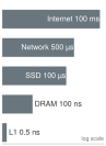
Access latency spans eight orders of magnitude, cache to internet.
The latency gap between on-chip registers and remote storage spans over eight orders of magnitude, making unbuffered I/O requests catastrophic for GPU accelerator utilization. Scaling these microsecond delays to intuitive human timeframes (table 9) makes the penalty of an un-cached fetch immediately visceral.
These latency numbers were popularized by Jeff Dean’s influential 2009 LADIS keynote.34 They explain why a poorly designed storage architecture can leave an expensive accelerator idle, and why distributed training requires careful attention to data locality.
34 Jeff Dean: Google Senior Fellow, architect of MapReduce, BigTable, Spanner, and TensorFlow. His 2009 LADIS keynote distilled the numbers in table 9 into the engineering heuristic that an L1 cache reference (0.5 ns) and a cross-data center round trip (150 ms) span a \(3 \times 10^{8}\) ratio – eight orders of magnitude that explain why a training pipeline reading features from remote storage instead of local NVMe starves the accelerator it was meant to feed.
| Operation | Latency (ns) | Human Scale | ML System Impact |
|---|---|---|---|
| L1 Cache Reference | 0.5 | 1 second | Immediate |
| L2 Cache Reference | 7 | 14 seconds | Fast computation |
| Main Memory (DRAM) | 100 | 3 minutes | The “memory wall” threshold |
| SSD (local NVMe) | 100,000 | 2 days | Data loading bottleneck |
| Network (same DC) | 500,000 | 11.57 days | Distributed coordination lag |
| SSD (remote network) | 2,000,000 | 46.30 days | Training-serving skew source |
| Object Store (S3) | 20,000,000 | 1 year | Archival access |
| Internet (CA to VA) | 100,000,000 | 6 years | Global user experience |
Access pattern alone does not exhaust the storage problem. ML workloads also store artifacts that conventional databases and warehouses were not designed around, and those artifacts shape infrastructure decisions across the entire development lifecycle, from experimental notebooks to production serving systems handling millions of requests per second.
Modern ML models contain millions to trillions of parameters requiring storage and retrieval patterns fundamentally different from traditional data. GPT-3 (Brown et al. 2020) requires approximately 700 GB for model weights when stored in FP32 format (175B parameters times 4 bytes), though practical deployments often use smaller numeric formats such as FP16 (350 GB) to reduce storage and access cost. Even at FP16 precision, this exceeds many organizations’ entire operational databases. The trajectory reveals accelerating scale: from AlexNet’s 60M parameters (Krizhevsky et al. 2012) to GPT-3’s 175B parameters (Brown et al. 2020), model size grew approximately 2916× in eight years. Storage systems must handle these dense numerical arrays efficiently for both capacity and access speed. Unlike typical files where sequential organization matters for readability, model weights benefit from block-aligned storage enabling parallel reads across parameter groups. When multiple accelerators need to read model data from shared storage, whether during training initialization or checkpoint loading, storage systems must deliver aggregate bandwidth approaching network interface limits, often 25 Gbps or higher, without introducing bottlenecks that would idle expensive compute resources. Model Compression later explains the model-side techniques that reduce these footprints further.
Brown, Tom B., Benjamin Mann, Nick Ryder, Melanie Subbiah, Jared Kaplan, Prafulla Dhariwal, Arvind Neelakantan, et al. 2020. “Language Models Are Few-Shot Learners.” Advances in Neural Information Processing Systems 33: 1877–901. https://doi.org/10.48550/arxiv.2005.14165.
Krizhevsky, Alex, Ilya Sutskever, and Geoffrey E. Hinton. 2012. “ImageNet Classification with Deep Convolutional Neural Networks.” Advances in Neural Information Processing Systems (NeurIPS) 25.
The iterative nature of ML development introduces versioning requirements qualitatively different from traditional software. Git excels at tracking code changes where files are predominantly text with small incremental modifications, but it fails for large binary files where even small model changes result in entirely new checkpoints. Storing ten versions of a 10 GB model naively would consume 100 GB; ML versioning systems typically keep lightweight metadata pointers in Git or a registry and store artifacts in external content-addressed storage. Identical files can be deduplicated, but changed binary checkpoints are often stored as separate objects unless the backend adds its own delta compression. Tools like DVC (Data Version Control) and MLflow maintain pointers to model artifacts rather than storing copies, enabling efficient versioning while preserving the ability to reproduce any historical model. A typical ML project generates hundreds of model versions during hyperparameter tuning—one version per training run as engineers explore learning rates, batch sizes, architectures, and regularization strategies. Without systematic versioning capturing training configuration, accuracy metrics, and training data version alongside model weights, reproducing results becomes impossible when yesterday’s model performed better than today’s but teams cannot identify which configuration produced it. This reproducibility challenge connects directly to the governance requirements addressed by section 1.7.4: regulatory compliance often requires demonstrating exactly which data and process produced specific model predictions.
Large-scale training generates substantial intermediate data requiring storage systems to handle concurrent read/write operations efficiently. When training jobs use multiple accelerators, each processing unit works on different portions of data, requiring storage systems to handle many simultaneous reads and writes. The specific patterns depend on the parallelization strategy employed, which Model Training examines in detail. From a storage perspective, systems must handle concurrent I/O at rates proportional to the number of processing units, with each potentially writing tens to hundreds of megabytes of intermediate results during model updates. For now, treat checkpoint files, optimizer-state snapshots, and explicit offload paths as large binary artifacts produced during training. Storage systems must provide low-latency access to support efficient coordination. If workers spend more time waiting for storage than performing computations, parallel processing becomes counterproductive regardless of the specific training approach used.
The bandwidth hierarchy that drove the coordination tax in section 1.5.3 constrains ML system design at every level, creating bottlenecks that no amount of compute optimization can overcome. While RAM delivers 50 to 200 gigabytes per second bandwidth on modern servers, network storage systems typically provide only one to ten gigabytes per second, and even high-end NVMe SSDs max out at one to seven gigabytes per second sequential throughput. Modern GPUs can process data faster than storage can supply it, creating scenarios where expensive accelerators idle waiting for data. Consider training an image classification model: loading 1,000 images per second at 150 KB each requires 150 MB/s sustained throughput from storage. When the GPU can process images faster than storage delivers them, the data pipeline, not the model, becomes the bottleneck. A 10-fold mismatch between GPU processing speed and storage bandwidth means expensive accelerators sit idle 90 percent of the time waiting for data. No amount of GPU optimization can overcome this I/O constraint.
Understanding these quantitative relationships enables informed architectural decisions about storage system selection and data pipeline optimization, which become even more critical during distributed training. Training throughput is bounded by the minimum of compute capacity and data supply rate: when storage cannot keep the accelerator fed, the bottleneck shifts from silicon to I/O.
Napkin Math 1.9: Storage bandwidth budget
Problem: What storage configuration keeps a reference accelerator from being data-starved while training ResNet-50? Hardware Acceleration explains the device family later; here, the point is how a compute ceiling becomes a data-path budget.
Start with the compute ceiling. The reference accelerator can deliver 312 TFLOP/s on dense FP16 operations. ResNet-50 costs about eight GFLOPs for each forward pass, and including the backward training pass raises the training-step cost to about 24.6 GFLOP per image. The training chapter derives that backward-pass machinery; here, the combined per-image cost is the input to the storage budget. When we divide accelerator peak by model cost, the calculation gives us an upper bound of 12,682 img/s.
That compute ceiling becomes a storage requirement once each image must arrive from disk or object storage. With 150 KB JPEG-compressed images, the data path must supply that many images per second times 150 KB per image, or approximately 1.9 GB/s.
The storage options now have a concrete target: saturating this accelerator requires 1.9 GB/s of sustained bandwidth.
- S3 Standard delivers about 100 MB/s per thread, so the pipeline needs 19 concurrent worker threads before software overhead.
- SATA SSDs deliver about 500 MB/s sequentially, making them a bottleneck for this accelerator.
- NVMe SSDs deliver approximately 5–7 GB/s, which is the right class of local storage for the target.
Systems insight: With SATA SSDs, maximum throughput is capped by 500 MB/s divided across 150 KB images, or approximately 3,333 img/s. The $15,000 GPU will run at 26 percent utilization because storage supplies only a small fraction of the accelerator’s image-processing ceiling. Storage physics dictates training speed.
Designing for high-throughput training starts by matching storage throughput to accelerator demand. This is the chapter’s starvation argument rotated to its third and final lens: section 1.1.3 priced the idle accelerator as a feeding tax, section 1.4.5 traced the same stall to CPU decode workers, and here the question becomes which storage tier can sustain the required supply rate.
The 500 MB/s figure represents effective SATA III sequential read throughput (the interface ceiling is 550 MB/s), and real-world random read performance with small files can be significantly lower. That caveat reinforces the general principle governing data pipelines: equation 5 bounds training throughput by compute capacity and the data supply rate defined in equation 6. Let \(R_{\text{train}}\), \(R_{\text{compute}}\), and \(R_{\text{data}}\) denote rates in samples per second; let \(B_{\text{storage}}\) be storage bandwidth in bytes per second, \(\eta_{\text{overhead}}\) the dimensionless fraction lost to overhead, and \(S_{\text{sample}}\) the bytes per sample. Under full overlap, the min-of-rates form corresponds to the \(T_{\text{step}} = \max(T_{\text{compute}}, T_{\text{io}})\) lower bound from section 1.4.5; with incomplete overlap, actual step time is higher. \[R_{\text{train}} \leq \min(R_{\text{compute}}, R_{\text{data}}) \tag{5}\] \[R_{\text{data}} = \frac{B_{\text{storage}}(1-\eta_{\text{overhead}})}{S_{\text{sample}}} \tag{6}\]
Once \(R_{\text{data}}\) is the smaller rate, additional accelerator compute cannot raise training throughput; the remedy must increase usable storage bandwidth or reduce bytes per sample.
When storage bandwidth becomes the limiting factor, teams must either improve storage performance through faster media, parallelization, or caching, or reduce the amount of data that must move. Large language model training may require processing hundreds of gigabytes of text per hour, while computer vision models processing high-resolution imagery can demand sustained data rates exceeding 50 gigabytes per second across distributed clusters. These requirements make data loading a systems-placement decision: framework data loaders parallelize I/O across asynchronous worker processes, using double-buffering prefetch queues to overlap the \(D_{\text{vol}}/\text{BW}_{\text{IO}}\) data fetch phase of batch \(k+1\) in host RAM while the accelerator computes the \(O/R_{\text{peak}}\) pass of batch \(k\) on GPU memory, preventing compute starvation stalls (\(L_{\text{lat}}\)). Framework loaders can also move expensive augmentation work closer to the accelerator rather than storing every augmented variant.
File format selection dramatically impacts the data term \(\left(\frac{D_{\text{vol}}}{\text{BW}}\right)\) of the iron law. Columnar formats like Parquet excel for tabular features by allowing column projection and pushdown filtering, whereas shard-based sequential formats like WebDataset or TFRecord pack millions of small binary objects (e.g., images or audio) into contiguous sequential streams. This sharding eliminates random disk seek overhead (\(L_{\text{lat}}\)), transforming slow random I/O into sustained sequential storage throughput (\(\text{BW}_{\text{IO}}\)). We can quantify this impact as format efficiency \((\eta_{\text{format}})\), which acts as a multiplier on effective bandwidth.
Napkin Math 1.10: Format efficiency
Storage formats determine how much “waste” data must move to retrieve the signal needed for training. Let \(\eta_{\text{format}}\) be the dimensionless fraction of bytes read that carry selected features, from 0 to 1. Equation 7 shows how that fraction scales physical bandwidth into usable pipeline bandwidth: \[ \text{Effective Bandwidth} = \text{Physical Bandwidth} \times \eta_{\text{format}} \tag{7}\] Values below 1 mean the format spends part of the physical data path on irrelevant bytes; improving layout can therefore raise usable throughput without changing the storage device.
Scenario: Training a fraud model using 20 features from a 100-column table.
Row-oriented (CSV) storage must read all 100 columns to get the 20 needed, giving a useful-byte fraction of 0.2 and wasting 80 percent of disk bandwidth. Column-oriented (Parquet) storage reads only the needed columns, so \(\eta_{\text{format}} \approx\) 1 ignoring metadata overhead, and the pipeline gets 5× higher effective throughput.
Systems insight: In this projection-only scenario, switching from CSV to Parquet provides the same effective read-throughput gain as a 5× faster data path. Row vs. columnar formats treats row vs. columnar storage layouts and the algebra of data operations (selection, projection, join) in depth.
Format choice follows the workload’s access pattern. When a large tabular dataset cannot be moved cheaply and training reads only selected columns, a columnar format reduces the bytes read per step.
Columnar storage formats like Parquet or Optimized Row Columnar (ORC) realize this reduction, five to ten times for typical ML workloads, through two mechanisms: the column projection the format-efficiency calculation just quantified, and column-level compression exploiting value patterns within columns. Column compression proves particularly effective for categorical features with limited cardinality: a country code column with 200 unique values in 100 million records compresses 20 to 50 times through dictionary encoding, while run-length encoding compresses sorted columns by storing only value changes. The combination can achieve total I/O reduction of 20 to 100 times compared to uncompressed row formats, directly translating to faster training iterations and reduced infrastructure costs.
Compression algorithm selection involves trade-offs between compression ratio and decompression speed. While gzip achieves higher compression ratios of six to eight times, Snappy achieves only two to three times compression but decompresses at 500 MB/s, roughly 4.2× faster than gzip’s 120 MB/s. For ML training where throughput matters more than storage costs, Snappy’s speed advantage often outweighs gzip’s space savings. Training on a 100 GB dataset compressed with gzip requires 13.9 minutes of decompression time, while Snappy requires only 3.3 minutes. When training iterates over data for 50 epochs, this 10.6 minutes difference per epoch compounds to 9 hours total, potentially the difference between running experiments overnight vs. waiting multiple days for results. The choice cascades through the system: faster decompression enables higher input throughput, reduced buffering requirements (less decompressed data needs staging), and better GPU utilization (less time idle waiting for data).
Storage performance optimization extends beyond format and compression to data layout strategies. Data partitioning based on frequently used query parameters dramatically improves retrieval efficiency. A recommendation system processing user interactions might partition data by date and user demographic attributes, enabling training on recent data subsets or specific user segments without scanning the entire dataset. Partitioning strategies interact with distributed training patterns: range partitioning by user ID enables data parallel training where each worker processes a consistent user subset, while random partitioning ensures workers see diverse data distributions. The partitioning granularity matters: too few partitions limit parallelism, while too many partitions increase metadata overhead and reduce efficiency of sequential reads within partitions. Poor partitioning compounds these problems in multi-accelerator training: when a distributed data-parallel job assigns shards to workers, imbalanced partition sizes cause straggler effects where the slowest reader holds up the entire gradient synchronization step. If all workers in an eight-accelerator job finish loading their batch in 12 ms but one slow worker reads from an oversized partition and takes 180 ms, that straggler determines the effective batch time. Well-partitioned datasets where each shard fits a worker’s local read budget and can be fetched without contending on a shared file handle are therefore a prerequisite for keeping distributed accelerator utilization high, a concern examined further in Model Training.
Storage across the ML lifecycle
Storage requirements evolve because each lifecycle stage asks the same data to serve a different access pattern. The same dataset is accessed through random sampling during exploratory analysis, sequential scanning during model training, and random access during production serving. These diverse patterns require storage architectures that accommodate all three access modes.
During development, flexibility matters more than raw performance. The key challenge is managing dataset versions without overwhelming storage capacity: ten experiments on a 100 GB dataset would naively require 1 TB of copies. The metadata-pointer mechanism introduced for model checkpoints in section 1.7.2 applies unchanged: tools like DVC track versions through pointers and content-addressed artifact storage, deduplicating identical content when possible. Governance considerations demand tiered access controls where synthetic or anonymized datasets are broadly available for experimentation, while production data containing sensitive information requires approval and audit trails.
Training phase requirements shift dramatically toward throughput. Modern deep learning processes massive datasets repeatedly across dozens or hundreds of epochs, making I/O efficiency critical. Training ResNet-50 on ImageNet across eight GPUs at 40,000 img/s would require roughly 6 GB/s for 150 KB compressed images, and substantially more if decoded FP32 tensors are staged. Storage unable to sustain this throughput idles GPUs, directly increasing infrastructure costs. The feature computation placement trade-off (section 1.4.5.3) is especially acute here: precomputing features achieves 30× storage reduction (150 KB to 5 KB vectors) but introduces staleness risk when extraction logic changes.
Deployment and real-time inference requirements prioritize low-latency random access. A recommendation system serving 10,000 req/s with 10 ms latency budgets and 10 feature reads/request requires 100,000 IOPS; meeting that illustrative target may require an in-memory database such as Redis, aggressive caching, or a purpose-built distributed key-value service. Edge deployment adds further constraints: limited device storage, intermittent connectivity, and the need for model updates without disrupting inference, typically addressed through tiered storage where models cache locally while reference data pulls from the cloud. Model versioning must support smooth transitions between versions, rapid rollback, and serving multiple versions simultaneously for A/B testing, operational patterns examined in ML Operations. Those serving and rollback guarantees depend on provenance: the system must know the exact dataset version behind each model version.
Data versioning for ML reproducibility
Suppose a recommendation model’s click-through rate drops after a routine weekly retraining even though the code has not changed. The team must distinguish among a data change, a labeling shift, and a corrupted upstream table. Without a record linking the model to the exact dataset that produced it, the team may spend days bisecting possibilities. With data versioning, they can diff the training snapshots and identify an upstream backfill that shifted the label distribution. Listing 3 shows the mechanism: Git records the small pointer file, DVC moves the large data bytes to remote storage, and a later checkout restores the exact training snapshot paired with the code commit (Iterative 2024).
git checkout and dvc checkout commands.
# Add data to version control
dvc add data/training.csv
git add data/training.csv.dvc
git commit -m "Add training data v1"
dvc push  # Upload to remote storage

# Later: retrieve exact data for any historical commit
git checkout abc123
dvc checkout  # Restores exact data from that commit
Data versioning is the storage analogue of source-control provenance. It connects model versions to exact training data, enabling debugging and reproducibility. Without it, teams cannot identify the exact data that trained the model now misbehaving in production.
DVC (Data Version Control) provides Git-like semantics for file snapshots (Iterative 2024), while listing 4 demonstrates Delta Lake’s transaction-log-based historical queries (Armbrust et al. 2020).
Iterative. 2024. Data Version Control (DVC).
-- Query data as it existed on a specific date
SELECT * FROM training_data TIMESTAMP AS OF '2024-01-15'

-- Or by version number for programmatic access
SELECT * FROM training_data VERSION AS OF 47
Two complementary capabilities complete the versioning infrastructure. Feature store point-in-time retrieval maintains historical feature values, enabling training with features “as they existed” at prediction time and preventing label leakage, the accidental use of information that would not be available when the prediction is made. Model registry integration links each model registry entry, a catalog record for a model artifact and its metadata, to its provenance: Git commit hash, data version, feature snapshot timestamp, and training configuration. Applied to the click-through-rate drop that opened this section, complete records can turn an open-ended search into a direct snapshot comparison that exposes the upstream backfill.
Long-term maintenance introduces a final storage consideration: retaining enough data to debug issues while honoring privacy, cost, and applicable record-keeping requirements. A high-volume recommendation system may use tiered retention: hot storage for rapid analysis, warm storage for periodic review, and cold archive storage for approved long-term investigations or records. Retention periods and immutability requirements depend on the data, jurisdiction, product, and risk; keeping everything indefinitely is neither a universal compliance rule nor a sound default.
Storage architecture determines where data resides and how it is retrieved, but physical storage layout alone cannot guarantee that features computed during batch training match those served in real time. Bridging batch training environments and low-latency serving systems requires specialized infrastructure designed for dual-access consistency.
Feature stores
The fundamental challenge of production feature management is preserving semantic consistency across environments: serving historical feature values for training and current feature values for inference. Point-in-time correctness is one reason teams adopt feature stores, which can reduce training-serving skew and enable feature reuse across models and teams. They do not eliminate skew by themselves; timestamp handling, backfills, freshness, and offline-online synchronization must still be correct.
The core problem feature stores address becomes clear when examining typical ML development workflows. During model development, data scientists write feature engineering logic in notebooks or scripts, often using different libraries and languages than production serving systems. Training might compute a user’s “total purchases last 30 days” using SQL aggregating historical data, while serving computes the same feature using a microservice that incrementally updates cached values. These implementations should produce identical results, but subtle differences in handling timezone conversions, dealing with missing data, or rounding numerical values cause training and serving features to diverge. Uber’s Michelangelo platform description treats training-serving skew and reusable feature pipelines as central production concerns, motivating an integrated platform approach to feature management (Hermann and Del Balso 2017).
Definition 1.4: Feature store
Feature store is the architectural layer that centralizes the management of machine learning features, decoupling feature computation from consumption.
- Significance: It supports point-in-time-correct historical retrieval for training \((x_{t-\Delta})\) and coordinated feature definitions for real-time inference \((x_t)\), reducing training-serving skew when timestamps, backfills, freshness, and synchronization are handled correctly.
- Distinction: Unlike a general-purpose database, a feature store is designed for dual storage modes: an offline store (columnar/batch) for training and an online store (key-value/low-latency) for serving.
- Common pitfall: A frequent misconception is that a feature store is only “a place to store data.” In reality, it manages feature definitions, values, and retrieval; transformation may run in the feature store, an offline store, or a separate batch or stream-compute engine.
Feature stores (discussed architecturally in Feature stores) provide a shared source of truth for feature definitions, supporting consistency across the ML lifecycle. When data scientists define a feature like user_purchase_count_30d, the feature store can maintain the definition (SQL query, transformation logic, or computation graph) and provide historical values for training and current values for serving. This architectural pattern reduces a class of subtle bugs that prove notoriously difficult to debug because models train successfully but perform poorly in production without obvious errors. The same centralized approach enables feature reuse across models and teams: when multiple teams build models requiring similar features, the feature store can prevent each team from reimplementing identical computations with subtle variations. A recommendation system might compute user embedding vectors across hundreds of dimensions, aggregating months of interaction history. Rather than each model team recomputing these expensive embeddings, the feature store can compute them once and serve them to multiple consumers.
The architectural pattern typically implements dual storage modes optimized for different access patterns. The offline store uses columnar formats like Parquet on object storage, optimized for batch access during training where sequential scanning of millions of examples is common. The online store uses key-value systems like Redis, optimized for random access during serving where individual feature vectors must be retrieved in milliseconds. Synchronization between stores becomes critical. As training generates new models using current feature values, those models deploy to production expecting the online store to serve consistent features. Feature stores typically implement scheduled batch updates propagating new feature values from offline to online stores, with update frequencies depending on feature freshness requirements.
Time-travel capabilities distinguish sophisticated feature stores from simple caching layers. Training requires accessing feature values as they existed at specific points in time rather than current values. Consider training a churn prediction model: for users who churned on January 15th, the model should use features computed on January 14th, not current features reflecting their churned status. Point-in-time correctness ensures training data matches production conditions where predictions use currently-available features to forecast future outcomes. Implementing time-travel requires storing feature history, not just current values, substantially increasing storage requirements but enabling correct training on historical data.
Feature store performance characteristics directly impact both training throughput and serving latency. The offline store must support high-throughput batch reads (millions of feature vectors per minute) using columnar formats that enable efficient reads of specific features from wide tables. The online store must support thousands to millions of reads per second with single-digit millisecond latency. In production, feature freshness adds further pressure: when users add items to shopping carts, recommendation systems need updated features within seconds, not hours. Streaming feature computation pipelines address this by updating online stores continuously rather than through periodic batch jobs, though streaming introduces complexity around exactly-once processing semantics—ensuring each event updates state once despite retries—and handling late-arriving events.
A fully assembled pipeline covering acquisition, ingestion, processing, labeling, and storage might suggest that data engineering work is “done.” Production systems, however, do not stand still. User behavior drifts, upstream schemas evolve, labeling guidelines change, and the pipeline engineering described in earlier sections gradually erodes unless actively maintained.
Self-Check: Question
An ML systems architect must select storage backends for three distinct workloads: (1) Millisecond point lookups of user feature vectors during real-time online serving; (2) High-throughput sequential scans over tabular fraud features during batch training; (3) Storing petabytes of raw, unstructured multi-modal audio and video recordings. Which mapping of storage architectures to workloads is optimal?
- Low-latency transactional database / key-value store; (2) Columnar data warehouse; (3) Scalable cloud data lake (object storage).
- Cloud object storage (S3); (2) Key-value database; (3) Columnar data warehouse.
- Columnar data warehouse; (2) Cloud data lake; (3) Low-latency transactional database.
- Scalable cloud data lake; (2) Low-latency transactional database; (3) Columnar data warehouse.
How does a feature store’s point-in-time correctness (time-travel join) prevent data leakage during offline training dataset generation?
- It encrypts historical feature values so that model weights cannot memorize training labels.
- It forces all features to be computed strictly in real time on the client device during model inference.
- It converts all timestamps into UTC strings to prevent database indexing errors.
- It reconstructs feature values exactly as they existed at the observation timestamp of each training event, preventing future feature values from leaking into historical training records.
Explain the storage-bandwidth bottleneck when feeding accelerators directly from cloud object storage versus local NVMe SSDs, and describe the common architectural caching pattern used to resolve it.
True or False: In a columnar storage format like Apache Parquet, reading 10 columns out of a 100-column table requires scanning the entire uncompressed row payload from disk.
Arrange the storage tiers across the ML lifecycle in their natural operational progression, from raw data capture to online inference serving:
- Online feature store (low-latency key-value store for inference)
- Offline feature store (point-in-time historical feature registry)
- Fast local NVMe cache on accelerator compute nodes
- Raw data lake (immutable object storage staging)
- Curated transactional table layer (lakehouse / warehouse)

Fallacies and Pitfalls
From acquisition through storage, every pipeline stage introduces opportunities for both excellence and failure. The following fallacies and pitfalls distill the most consequential misconceptions that lead teams astray.
Fallacy: More data always improves model performance.
Beyond a threshold, additional data yields diminishing returns. Empirical studies across image classification, translation, and language modeling confirm that test loss often follows a power law in dataset size, so each additional tranche of data produces progressively smaller gains (Hestness et al. 2017). The task-relevant signal heuristic from section 1.1 reflects the same systems trade-off: redundant examples can add data-processing cost while contributing little new task-relevant information.
Hestness, Joel, Sharan Narang, Newsha Ardalani, Gregory Diamos, Heewoo Jun, Hassan Kianinejad, Md. Mostofa Ali Patwary, Yang Yang, and Yanqi Zhou. 2017. “Deep Learning Scaling Is Predictable, Empirically.” arXiv Preprint arXiv:1712.00409.
Pitfall: Planning petabyte migration as a bandwidth-only transfer.
Engineers may estimate migration time by dividing dataset size by network bandwidth, but data gravity (section 1.1) also pulls in pipeline re-engineering, data-quality revalidation, schema migration, lineage updates, and synchronization of dependent services. Petabyte-scale migrations can therefore require substantially more engineering time than wire time.
Fallacy: Data preprocessing can be finished once and left alone.
Data distributions can drift as user behavior, market conditions, and upstream systems evolve. A preprocessing pipeline validated at launch can become stale as the world changes around it. Production systems require monitoring and evidence-based responses, not one-time validation.
Pitfall: Ignoring data serialization cost.
Teams can meticulously optimize accelerator kernels while leaving data loading as JSON or CSV. Text formats can add parsing and byte-transfer overhead relative to binary formats, while columnar formats such as Parquet reduce I/O when tabular workloads read only a subset of columns. Benchmark formats against the actual access pattern and convert when the measured savings justify the migration.
Fallacy: High training accuracy indicates production readiness.
Training accuracy measures fit to historical data; held-out evaluation estimates generalization under its sampled conditions, while production performance depends on the live environment. Training-serving skew, distribution shift, and coverage gaps can make a model with strong validation results perform poorly after deployment. The debugging flowchart in figure 15 exists because diagnosing that gap requires tracing data and system conditions, not trusting one aggregate score.
Pitfall: Ignoring training-serving skew until deployment.
Feature-computation differences between training and serving environments are one important cause of ML deployment failures. By the time skew manifests in production metrics, debugging can become difficult. Feature stores and consistency contracts should be considered early rather than only after deployment incidents.
Fallacy: Synthetic data can fully replace real-world data collection.
Synthetic data can augment real observations by targeting rare cases, controlled variations, or privacy-sensitive scenarios, but its value depends on fidelity to the deployment task. Generation inherits omissions and artifacts from its models and assumptions. A KWS system trained only on synthesized speech may miss accents, background noises, and pronunciation variations absent from the generator. Teams should validate the real-synthetic mixture against representative deployment data rather than assume a universally optimal recipe.
Pitfall: Neglecting data versioning until model debugging requires it.
Teams may defer data versioning until a deployed model produces unexpected results. Without versioning, reproducing a training run requires reconstructing the exact inputs or re-executing the pipeline. Consider a model that performed well three months ago but degrades after retraining on updated data. Without versioned snapshots, the team cannot determine whether the regression stems from a labeling policy change, a schema migration error, or genuine distribution shift. The data lineage principles established in section 1.5.4 formalize this requirement: every training artifact must trace back to a specific, immutable dataset version. Deferring versioning lengthens debugging because each investigation must first identify the exact data that trained the model.
Self-Check: Question
An engineering team assumes that doubling their raw dataset volume by web scraping uncurated text and generating synthetic speech samples will automatically improve downstream model accuracy. According to the chapter’s fallacies and pitfalls, why is this assumption flawed?
- Because scaling laws exhibit diminishing returns (power-law test loss flattening), and adding uncurated or synthetic data can increase data gravity and transport energy while introducing generator domain gaps and noise.
- Because neural networks cannot mathematically process more than one million training records without floating-point overflow.
- Because synthetic data is legally prohibited from being combined with real-world sensor captures.
- Because web scraping always converts binary audio files into plain text formats, corrupting feature representations.
Explain why planning a petabyte-scale dataset migration solely as a network wire transfer (\(T = D_{\text{vol}}/\text{BW}\)) is a major systems pitfall.
True or False: Achieving high accuracy on a randomly split validation set during model development proves that the system will perform reliably after deployment.
Summary
Data engineering provides the foundational infrastructure that transforms raw information into the basis of machine learning systems, determining model performance, system reliability, ethical compliance, and long-term maintainability. The four pillars framework of Quality, Reliability, Scalability, and Governance organizes design choices across acquisition, ingestion, validation, and storage, while the cascading nature of data quality failures reveals why every pipeline stage requires careful engineering decisions. The task of “getting data ready” encompasses complex trade-offs quantified throughout this chapter: data engineering cost constants for budgeting, storage performance hierarchies, and drift detection thresholds that operationalize the degradation equation into production monitoring infrastructure.
Key Takeaways: Data is the source code
- Data cascades make upstream quality the highest-leverage investment: Collection errors amplify through every pipeline stage (figure 1). The four pillars (Quality, Reliability, Scalability, Governance) organize prevention, while documentation, schema, quality, and freshness debt require continuous remediation.
- Data is code; version it, test it, review it: A dataset is source code for an ML system. Apply the same rigor through version control, validation tests, and data review.
- Training-serving consistency is nonnegotiable: Feature transformations shared by training and serving must have equivalent semantics and reuse the same learned state, such as normalization constants and vocabulary mappings.
- Pipeline architecture choices have large cost implications: Streaming costs more to operate than batch, while ETL trades storage savings for greater schema-change overhead. Select ingestion patterns by the value of latency, not the appeal of real time.
- Labeling costs dominate and require substantial resource allocation: Labeling can cost hundreds to more than a thousand times one optimized training run; in the reference calculation in section 1.3.2, the ratio is 521×–1,562×. Labeling can remain a costly scheduling bottleneck even when annotation work is parallelized.
- Storage hierarchy determines iteration speed: The 50× throughput gap between local NVMe (5 GB/s) and cloud object storage (100 MB/s) determines whether iterations occur daily or weekly.
- The degradation equation becomes actionable through drift and outcome monitoring: Divergence metrics such as KL measure changes between \(P_t\) and \(P_0\), while labeled outcomes or validated proxies determine whether those changes correspond to model degradation.
The KWS case study combines curated, crowdsourced, and synthetic acquisition; consistency validation; tiered storage for 23.4 million audio samples across 748.8 GB of raw data; and lineage for always-listening devices. Data engineering is not preprocessing before “real” ML work; it underpins model performance, user trust, and regulatory compliance.
What’s Next: From source code to executable
The data pipeline has produced a clean, versioned training set, but a dataset teaches nothing on its own. Neural Computation opens that black box to examine the algorithm axis: the mathematical operations that convert prepared examples into learned behavior and make neural networks predictable, debuggable, and optimizable.
Self-Check: Question
Reflecting on the chapter’s quantitative summaries, which two systems constants highlight the dominant economic and performance bottlenecks in modern ML data engineering?
- GPU arithmetic execution is \(1{,}000\times\) more expensive than data labeling, and object storage is \(50\times\) faster than local NVMe SSDs.
- Data labeling costs dominate compute by \(500\times\text{--}1{,}000\times\) the cost of an optimized training run, and local NVMe SSDs provide a \(50\times\) bandwidth advantage over cloud object storage.
- Network egress costs are always zero, and database row scans are faster than columnar Parquet reads.
- Feature stores eliminate 100% of memory requirements, and audio preprocessing requires more memory than model weights.
Summarize why training data must be treated as the ‘source code’ of an ML system, and describe the core responsibilities of data engineering in managing this source code across its lifecycle.
Arrange the primary operational phases of the end-to-end ML data engineering lifecycle in their canonical order:
- Strategic data acquisition and gap closing
- Ingestion, schema validation, and defensive quality checks
- Idempotent transformation and feature engineering
- Labeled dataset compilation and consensus verification
- Strategic storage tiering and feature store materialization
- Continuous operational health monitoring and data debt remediation
Self-Check Answers
Self-Check: Answer
A machine learning team maintains a \(1\text{ PB}\) raw training corpus in a US East cloud storage bucket and provisions a dedicated compute cluster in US West. The regions are connected by a dedicated \(100\text{ Gbps}\) network fabric. Cloud egress pricing is $0.02/, and the model training run takes \(20\text{ hours}\). Under the principles of data gravity and transfer economics (\(T = D_{\text{vol}}/\text{BW}\)), which architecture should the team select?
- Stream the dataset remotely across the link during training, because a 100 Gbps network provides sufficient throughput to prevent GPU I/O stalls.
- Partition the dataset equally across both cloud regions so that each region trains half the model asynchronously without transfer fees.
- Apply standard gzip compression to eliminate data gravity, enabling real-time remote streaming at zero net cost.
- Provision or relocate compute in US East near the data, because transferring 1 PB requires ~22.2 hours and incurs ~$20,000 in egress fees, exceeding the training run’s time and budget.
Answer: The correct answer is D. Provision or relocate compute in US East near the data, because transferring 1 PB requires ~22.2 hours and incurs ~$20,000 in egress fees, exceeding the training run’s time and budget. Transferring \(1\text{ PB}\) (\(1\text{ PB} = 10^6\text{ GB} = 8 \times 10^6\text{ Gb}\)) over a \(100\text{ Gbps}\) link requires \((8 \times 10^6) / 100 = 80{,}000\text{ s} \approx 22.2\text{ hours}\), which exceeds the \(20\text{ hour}\) training job itself, while incurring \(10^6\text{ GB} \times \$0.02/\text{GB} = \$20{,}000\) in network egress costs. When dataset mass makes \(D_{\text{vol}}/\text{BW}\) dominate compute duration and cost, data gravity dictates that compute must move to data. Streaming over the wide-area link stalls training because wire time exceeds compute time; splitting across regions still requires synchronization or cross-region transfers; and gzip cannot deliver the orders-of-magnitude reduction needed to overcome the physical bottleneck.
Learning Objective: Calculate transfer time (\(D_{\text{vol}}/\text{BW}\)) and network egress costs to evaluate compute placement under data gravity constraints.
A computer vision model training on an accelerator cluster consumes images at \(3{,}119\text{ img/s}\), demanding \(1.9\text{ GB/s}\) of sustained input streaming bandwidth. However, the host DataLoader reads from a standard cloud block storage volume delivering only \(125\text{ MB/s}\). According to the chapter’s feeding tax analysis, what is the resulting operational state of the system?
- The accelerator suffers a feeding tax of >90% (spending over 90% of its wall-clock time idle waiting for I/O), severely degrading hardware efficiency _{}.
- The accelerator remains 100% compute-bound because internal GPU tensor execution is mathematically decoupled from storage I/O.
- Increasing the per-device batch size by 8x will completely eliminate the I/O bottleneck without requiring storage upgrades.
- Host memory caches automatically compensate for the throughput gap after the first epoch without any CPU overhead.
Answer: The correct answer is A. The accelerator suffers a feeding tax of >90% (spending over 90% of its wall-clock time idle waiting for I/O), severely degrading hardware efficiency {}. The feeding tax measures the fraction of wall-clock time an accelerator spends stalled on I/O: delivering \(125\text{ MB/s}\) (\(0.125\text{ GB/s}\)) when \(1.9\text{ GB/s}\) is demanded yields an effective feeding efficiency {} / 1.9 %, meaning the accelerator experiences a feeding tax of $(1 - 0.066) % %. The claim that tensor execution is decoupled from storage ignores pipeline starvation; scaling batch size increases per-step data volume without resolving the sustained transfer deficit; and host caching cannot overcome baseline disk bandwidth during cold or out-of-core scans.
Learning Objective: Calculate the feeding tax and analyze how I/O bandwidth deficits degrade accelerator hardware efficiency.
Using the data selection gain formula ( ) and the energy-movement invariant, explain why pruning 50% of redundant samples via deduplication provides high systems leverage even when per-batch model execution is compute-bound.
Answer: Selection gain is the ratio of useful task signal to data mass (\(D_{\text{vol}}\)). Pruning \(50\%\) redundant data doubles the selection gain by halving total bytes moved and stored without sacrificing learned accuracy. Furthermore, by the energy-movement invariant, moving a 32-bit value across DRAM (\(100\text{--}200\text{ pJ}\)) or network (\(100{,}000\text{ pJ}\)) costs \(100\times\) to \(100{,}000\times\) more energy than an on-chip FP32 multiply (~\(1\text{ pJ}\)). Halving dataset volume eliminates massive off-chip data transport energy, DataLoader decompression load, and persistent storage fees across every training epoch.
Learning Objective: Analyze the systems benefits of dataset deduplication using the data selection gain ratio and the energy-movement hierarchy.
**According to the chapter’s energy-movement hierarchy, arrange the following operations in ascending order of energy consumed per 32-bit value (from lowest energy to highest energy):
- Local NVMe SSD access
- On-chip 32-bit FP multiply
- Wide-area network transfer
- Off-chip DRAM memory access**
Answer: The correct order is: (2) On-chip 32-bit FP multiply -> (4) Off-chip DRAM memory access -> (1) Local NVMe SSD access -> (3) Wide-area network transfer. An on-chip 32-bit floating-point multiply costs ~\(1\text{ pJ}\) (baseline \(1\times\)). Moving a 32-bit value from off-chip DRAM costs ~\(100\text{--}200\text{ pJ}\) (~\(100\times\)). Reading a 32-bit value from a local NVMe SSD costs ~\(1{,}000\text{--}2{,}000\text{ pJ}\) (~\(1{,}000\times\)). Transferring a 32-bit value across a data-center network costs ~\(100{,}000\text{ pJ}\) (~\(100{,}000\times\)).
Learning Objective: Compare storage and compute operations across the memory hierarchy by their relative energy cost per bit.
The wall-clock time lost by high-throughput accelerators while waiting for input batches from slow storage pipelines is formally termed the ____.
Answer: The correct answer is feeding tax (or the feeding tax). The feeding tax quantifies the reduction in hardware efficiency (_{}) caused by I/O bottlenecks where storage and data-loading flow rates cannot keep pace with accelerator consumption.
Learning Objective: Explain the technical definition and systems impact of the feeding tax in ML data pipelines.
Self-Check: Answer
An always-on Keyword Spotting (KWS) system on an embedded voice assistant continuously evaluates 1-second audio classification windows (\(24\text{ hours/day}\) over a \(30\text{-day}\) month). The product specification mandates an SLA of at most 1 false activation per month. An engineer suggests that achieving a standard 99% accuracy (a 1% false positive rate on background noise) is sufficient. How many false activations would a 1% FPR produce per month, and what per-window FPR is actually required?
- A 1% FPR produces 720 false activations per month; the SLA requires a per-window FPR of \(\le 1.38 \times 10^{-5}\).
- A 1% FPR produces ~25,920 false activations per month (~36 false wakes/hour); the SLA requires a per-window FPR of \(\le 3.86 \times 10^{-7}\) (>99.9999% non-keyword rejection).
- A 1% FPR produces ~2,592 false activations per month; the SLA requires a per-window FPR of \(\le 1.0 \times 10^{-4}\).
- A 1% FPR satisfies the SLA because accuracy is averaged over the total number of audio hours across the entire device fleet.
Answer: The correct answer is B. A 1% FPR produces ~25,920 false activations per month (~36 false wakes/hour); the SLA requires a per-window FPR of \(\le 3.86 \times 10^{-7}\) (>99.9999% non-keyword rejection). Over a 30-day month with continuous 1-second windows, there are \(30 \times 24 \times 3600 = 2{,}592{,}000\) evaluation windows. A 1% false-positive rate yields \(0.01 \times 2{,}592{,}000 = 25{,}920\) false wake-ups per month (roughly 36 false activations every hour, rendering the device unusable). To meet the SLA of \(\le 1\) false activation per month, the per-window FPR must satisfy \(\text{FPR} \le 1 / 2{,}592{,}000 \approx 3.86 \times 10^{-7}\), requiring \(>99.9999\%\) non-keyword rejection. The other options miscalculate the monthly window count or incorrectly assume standard aggregate classification metrics apply directly to streaming continuous inference.
Learning Objective: Calculate the required per-window false positive rate for always-on streaming ML systems and explain why aggregate accuracy fails for streaming workloads.
A data engineering team implements comprehensive synchronous schema and distribution validation checks directly inside the real-time event ingestion path. Under the Four Pillars framework, which primary operational trade-off will this team encounter?
- A Governance trade-off: inspecting payload schemas automatically breaches user data retention agreements.
- A Model Capacity trade-off: validating input records forces downstream neural network layers to increase parameter counts.
- A Scalability and Reliability trade-off: heavy synchronous validation consumes CPU cycles and increases per-record latency, reducing ingestion throughput and risking dropped messages during traffic spikes.
- A Durability trade-off: validating data records accelerates physical wear on persistent solid-state drive cells.
Answer: The correct answer is C. A Scalability and Reliability trade-off: heavy synchronous validation consumes CPU cycles and increases per-record latency, reducing ingestion throughput and risking dropped messages during traffic spikes. The Four Pillars framework highlights tension between Quality and Scalability/Reliability: performing exhaustive synchronous validation in the hot ingestion path adds CPU latency and backpressure, reducing peak throughput and creating potential availability failures under load surges. Production pipelines balance this by executing lightweight structural checks synchronously at ingestion while offloading deep statistical and semantic validation to asynchronous processing or dead-letter queues. The remaining choices misattribute the trade-off to privacy violations, neural parameter expansion, or SSD wear.
Learning Objective: Analyze the cross-pillar trade-offs between validation rigor (Quality) and processing throughput/latency (Scalability and Reliability).
Based on the DLRM Recommendation Lighthouse, describe how modern recommendation systems bifurcate data engineering resource demands between dense continuous signals and high-cardinality categorical IDs.
Answer: DLRM architectures split data demands into two divergent pipelines: (1) Dense continuous features require high-throughput streaming compute and dense matrix multiplications on accelerators; (2) High-cardinality categorical IDs (e.g., billions of user and item IDs) require terabyte-scale distributed embedding tables constrained by memory capacity and sparse memory-bandwidth lookups. Because these large embedding tables cannot fit on a single accelerator’s memory, data engineering must implement distributed table partitioning and caching strategies to mitigate sparse lookup bottlenecks.
Learning Objective: Explain the bifurcated scalability profile (memory capacity and sparse lookup bandwidth vs. dense compute) of modern recommendation system architectures.
True or False: Data cascades in ML systems are easily caught by standard software unit tests because corrupted input data causes deterministic assertion failures in pipeline code.
Answer: False. Data cascades are characterized as ‘silent’ failures precisely because corrupted or drifted data often remains syntactically valid (e.g., non-null strings or valid numeric ranges) and passes traditional code unit tests. The defect cascades downstream, subtly biasing feature distributions, distorting learned model representations, and degrading real-world accuracy without throwing software exceptions.
Learning Objective: Compare silent data cascade failure modes with traditional software bugs caught by unit tests.
**Trace the propagation sequence of a data cascade as described in the chapter, from its root cause to user-facing impact:
- Downstream model optimization on distorted representations
- Upstream sensor or schema change without contract notification
- Silent distortion of extracted features passing syntactic checks
- Degraded real-world predictions and costly post-deployment rollback**
Answer: The correct order is: (2) Upstream sensor or schema change without contract notification -> (3) Silent distortion of extracted features passing syntactic checks -> (1) Downstream model optimization on distorted representations -> (4) Degraded real-world predictions and costly post-deployment rollback. A data cascade begins with an uncoordinated upstream source or schema change. Because the data passes basic syntactic tests, it enters feature extraction and silently distorts intermediate representations. Downstream model training optimizes over these corrupted features, ultimately manifesting as degraded production predictions and requiring expensive system rollback.
Learning Objective: Analyze the multi-stage propagation of data cascades from upstream defects to production degradation.
Self-Check: Answer
An ML organization budgets for training a computer vision model across various data sourcing methods. Based on the chapter’s illustrative data engineering cost constants, which cost relationship correctly reflects the per-unit economics of data acquisition?
- Storing a terabyte of training data in cloud object storage for a month costs significantly more than obtaining a single expert medical annotation.
- Generating synthetic image samples is ten times more expensive per image than crowdsourced human classification.
- A single cloud GPU training hour ($2–4/hr) exceeds the cost of a full human review hour ($15–50/hr) by an order of magnitude.
- Expert medical labeling ($50–200 per study) and bounding-box annotations ($0.15–0.50 per box) are orders of magnitude more expensive per unit than S3 Standard storage (~$23/TB/month).
Answer: The correct answer is D. Expert medical labeling ($50–200 per study) and bounding-box annotations ($0.15–0.50 per box) are orders of magnitude more expensive per unit than S3 Standard storage (~$23/TB/month). Per-unit data engineering costs show that human annotation—especially domain expert labeling ($50–200/study) and dense spatial annotations ($0.15–0.50/box)—dominates project budgets, whereas raw object storage (~$23/TB/month) is cheap. Storing 1 TB in S3 is comparable to or cheaper than a single medical study label; synthetic generation is typically an order of magnitude cheaper (not more expensive) than manual collection; and human review hours ($15–50/hr) cost substantially more than spot GPU training hours ($2–4/hr).
Learning Objective: Compare per-unit data engineering cost constants across human labeling tiers, cloud storage, and compute resources.
Multiple independent autonomous driving teams train their perception models exclusively on a popular public driving benchmark. What systemic failure mode does this practice introduce into the broader ecosystem?
- Shared dataset bias propagation, where common blind spots, annotation artifacts, and unrepresented edge cases become correlated systemic weaknesses across all deployed models.
- Catastrophic memory leaks in GPU driver kernels caused by repeated reading of shared image formats.
- Immediate violation of data gravity constraints due to distributed multi-tenant reads.
- Automatic over-fitting to hardware memory hierarchies during distributed gradient synchronization.
Answer: The correct answer is A. Shared dataset bias propagation, where common blind spots, annotation artifacts, and unrepresented edge cases become correlated systemic weaknesses across all deployed models. When multiple models across an industry rely on a single common benchmark dataset, any systemic flaws (e.g., geographic bias, missing weather conditions, or consistent label errors) propagate across the entire ecosystem. Rather than producing independent models with diverse failure modes, the ecosystem develops correlated blind spots. The other options describe unrelated GPU memory bugs, network gravity violations, or hardware synchronization issues.
Learning Objective: Evaluate the ecosystem-wide risks of shared dataset bias propagation and benchmark over-reliance.
Discuss the primary advantages and critical risks of using synthetic data generation (e.g., 3D graphics rendering or generative audio simulation) as a core data acquisition strategy.
Answer: Advantages: Synthetic data provides scalable, low-cost training examples with perfectly accurate, automated ground-truth labels (e.g., exact 3D bounding boxes, depth maps, or audio SNR) and enables targeted generation of rare safety-critical edge cases. Risks: Synthetic generators inherit domain gaps and omissions from their underlying models; models trained purely on synthetic data often fail on real-world distributions due to missing acoustic reverberations, lighting variations, or demographic accents absent from the generator.
Learning Objective: Analyze the trade-offs between synthetic data scalability and real-world domain gaps in acquisition strategy.
True or False: Achieving state-of-the-art benchmark accuracy on a curated dataset (such as ImageNet or Common Voice) guarantees that an ML model is ready for deployment in real-world production environments.
Answer: False. Curated benchmarks provide standardized baselines for research comparison, but their distributions rarely capture the full variety of real-world deployment conditions (e.g., microphone hardware variations, regional acoustic noise, adversarial inputs, or demographic shifts). Models tuned specifically to benchmark distributions frequently suffer severe performance drops when exposed to uncurated production data.
Learning Objective: Explain why benchmark performance fails to guarantee real-world generalization across deployment distributions.
**According to the chapter’s gap-closing acquisition strategy, arrange the following sourcing options in the recommended escalation order (from lowest setup cost to highest cost/effort):
- In-house specialist/expert annotation
- Crowdsourced human annotation platforms
- Curated open-source benchmark reuse
- Programmatic web scraping and synthetic data generation**
Answer: The correct order is: (3) Curated open-source benchmark reuse -> (4) Programmatic web scraping and synthetic data generation -> (2) Crowdsourced human annotation platforms -> (1) In-house specialist/expert annotation. Data acquisition begins by evaluating preexisting curated datasets to establish a baseline and identify specific coverage gaps. If scale is the binding constraint, teams escalate to programmatic web scraping or synthetic data. When human judgment is required, crowdsourced platforms offer moderate cost, escalating finally to expensive in-house domain experts for high-stakes or ambiguous edge cases.
Learning Objective: Design an escalated data acquisition workflow that balances cost, scale, and annotation expertise.
Self-Check: Answer
A production monitoring system tracks feature distributions over time using the Population Stability Index (PSI). The incoming feature distribution for a key credit feature yields a PSI value of \(0.28\) compared to the baseline training distribution. According to standard operational drift bands, how should the data pipeline respond?
- No action is required because PSI values below 0.50 indicate negligible distribution change.
- Trigger a critical alert and initiate root-cause investigation or automated model retraining, because a PSI > 0.25 indicates significant distribution drift.
- Immediately drop all incoming records and halt the ingestion cluster with a fatal error.
- Switch the database storage format from Parquet to CSV to improve float precision.
Answer: The correct answer is B. Trigger a critical alert and initiate root-cause investigation or automated model retraining, because a PSI > 0.25 indicates significant distribution drift. Standard operational PSI thresholds establish three monitoring bands: < 0.10 indicates stability (no action); \(0.10 \le \text{PSI} \le 0.25\) indicates moderate drift (warning, monitor closely); and > 0.25 indicates significant distribution drift requiring urgent investigation, retraining, or pipeline remediation. Halting the ingestion cluster is inappropriate for statistical drift, and changing file formats has no bearing on feature distributions.
Learning Objective: Apply Population Stability Index (PSI) thresholds to detect feature drift and determine appropriate pipeline response protocols.
An ML engineering team is architecting an ingestion pipeline for tabular transaction data. They evaluate Extract-Transform-Load (ETL) versus Extract-Load-Transform (ELT). Which architectural trade-off correctly characterizes ELT in modern data lakehouses?
- ELT executes all transformations in memory on the edge device before transmitting bytes to cloud storage.
- ELT requires rigid upfront schema definitions (schema-on-write) and rejects any semi-structured data formats.
- ELT loads raw data directly into scalable lakehouse storage first and transforms it downstream using scalable query engines, preserving raw data history and decoupling ingestion from evolving feature logic.
- ELT eliminates the need for data governance and quality validation because transformations occur after storage.
Answer: The correct answer is C. ELT loads raw data directly into scalable lakehouse storage first and transforms it downstream using scalable query engines, preserving raw data history and decoupling ingestion from evolving feature logic. ELT decouples raw ingestion from transformation: raw events land directly in cheap, scalable storage (schema-on-read), allowing downstream engines (Spark, Presto) to execute feature transformations iteratively. This preserves historical raw inputs for future reprocessing and prevents upstream schema updates from blocking ingestion. In contrast, ETL transforms data before loading, which enforces schema-on-write but loses raw unstructured details and requires pipeline redeployments when feature definitions change. The remaining options mischaracterize edge compute, schema requirements, or governance needs.
Learning Objective: Compare ETL and ELT architectures regarding storage decoupled ingestion, schema evolution, and historical data retention.
Explain how combining a Circuit Breaker pattern with a Dead Letter Queue (DLQ) prevents cascading failures and data loss in streaming ML data ingestion pipelines.
Answer: A Circuit Breaker monitors failure rates (e.g., malformed payloads, timeout surges) and automatically trips to halt downstream processing when error thresholds are exceeded, preventing crashing downstream model services or overwhelming databases. A Dead Letter Queue (DLQ) captures and isolates unparsable or rejected records alongside error metadata without dropping them, allowing the primary pipeline to maintain throughput for valid traffic while engineers inspect and reprocess bad records asynchronously.
Learning Objective: Design reliable streaming data pipelines using Circuit Breaker and Dead Letter Queue (DLQ) patterns for fault isolation.
Using the 2016 Microsoft Tay chatbot incident, explain why public data ingestion surfaces require strict input validation, rate limiting, and adversarial filtering before data shapes model behavior.
Answer: Microsoft Tay ingested uncurated public user interactions from Twitter to adapt its responses. Adversarial users exploited this unfiltered public surface with coordinated toxic prompts, causing the bot to tweet abusive statements within 16 hours. The incident demonstrates that any public ingestion path directly influencing model behavior acts as a security attack surface, requiring robust content filtering, anomaly detection, adversarial input controls, and rate limits to prevent malicious data from corrupting the system.
Learning Objective: Analyze the security and safety implications of unvalidated public data ingestion using the Microsoft Tay war story.
An explicit, machine-enforceable agreement between data producers and data consumers that defines column types, value bounds, nullability, and distribution constraints is called a ____.
Answer: The correct answer is schema contract (or data contract). Schema contracts prevent upstream data drift from silently breaking downstream ML processing by enforcing type and semantic guarantees at integration boundaries.
Learning Objective: Explain schema contracts and their role in preventing breaking changes across ML data pipelines.
Self-Check: Answer
An engineer normalizes a numerical feature by computing standard \(z\)-scores: \(x' = (x - \mu)/\sigma\). During production serving, how must the parameters \(\mu\) and \(\sigma\) be handled to satisfy the Consistency Imperative and prevent training-serving skew?
- Persist the exact \(\mu\) and \(\sigma\) computed on the training dataset alongside the model artifact, loading and applying those fixed constants to live serving inputs.
- Recompute \(\mu\) and \(\sigma\) dynamically over each incoming serving batch to ensure the live data is always centered at zero.
- Discard \(\mu\) and \(\sigma\) entirely at inference time and rely on batch normalization layers inside the neural network.
- Compute \(\mu\) and \(\sigma\) independently over a rolling 1-hour window of serving traffic to track seasonal shifts.
Answer: The correct answer is A. Persist the exact \(\mu\) and \(\sigma\) computed on the training dataset alongside the model artifact, loading and applying those fixed constants to live serving inputs. The Consistency Imperative requires state synchronization across training and serving: transformation parameters computed during training (means, standard deviations, one-hot vocabularies, embedding lookups) must be persisted and reused during serving. Recomputing statistics dynamically over live batches or rolling windows alters the feature scale relative to what the model learned, creating training-serving skew and causing silent prediction degradation. Relying on neural batch normalization does not resolve pre-network input feature scaling.
Learning Objective: Apply the Consistency Imperative by synchronizing stateful transformation parameters between training and serving.
A distributed preprocessing job must compute global mean normalization across \(1\text{ TB}\) of feature data distributed evenly over 100 worker nodes. Architecture 1 gathers all \(1\text{ TB}\) of raw data to a central coordinator node over a \(1\text{ Gbps}\) network to compute the global mean. Architecture 2 computes a local sum and record count on each node (transferring only 16 bytes per node to the coordinator) and calculates the exact global mean locally. What is the systems trade-off and coordination tax difference?
- Centralized gathering is faster because centralizing all data eliminates worker-level floating-point rounding errors.
- Local aggregation produces only an approximation of the mean, whereas centralized gathering computes the true mathematical value.
- Both approaches take identical execution time because the total number of arithmetic additions is preserved.
- Centralized gathering incurs a massive coordination tax, taking ~8,000 seconds to transfer 1 TB over 1 Gbps, whereas local aggregation transfers under 2 KB of aggregated statistics in sub-seconds while computing the exact same mathematical mean.
Answer: The correct answer is D. Centralized gathering incurs a massive coordination tax, taking ~8,000 seconds to transfer 1 TB over 1 Gbps, whereas local aggregation transfers under 2 KB of aggregated statistics in sub-seconds while computing the exact same mathematical mean. Transferring \(1\text{ TB}\) (\(8{,}000\text{ Gb}\)) across a \(1\text{ Gbps}\) link takes \((8{,}000 / 1) = 8{,}000\text{ s} \approx 2.2\text{ hours}\) purely in network coordination tax. In contrast, local aggregation computes local partial sums \(\sum x_i\) and counts \(N_k\) on each node in parallel, transferring only 16 bytes per worker (\(100 \times 16\text{ B} = 1.6\text{ KB}\)), allowing the coordinator to compute the exact global mean \(\mu = (\sum \text{sum}_k) / (\sum N_k)\) in milliseconds. Local aggregation is mathematically exact (not an approximation) and exploits data locality.
Learning Objective: Calculate the coordination tax of distributed data processing and compare centralized gathering against local aggregation.
Define idempotency in the context of data transformation pipelines and explain why idempotent operations (such as upserts) are essential for fault recovery in distributed ML pipelines.
Answer: Idempotency means applying an operation multiple times produces the exact same system state as applying it once (\(f(f(x)) = f(x)\)). In distributed pipelines subject to network timeouts and worker crashes, retry mechanisms can execute the same task repeatedly; non-idempotent operations (such as appending rows) create duplicate records and corrupt gradient updates, whereas idempotent operations (such as database upserts or deterministic partition overwrites) allow safe retries without duplicating data.
Learning Objective: Explain the importance of idempotent transformations and deterministic pipelines for safe fault recovery.
True or False: Using the identical Python preprocessing function in both training and serving code repositories is sufficient to eliminate training-serving skew.
Answer: False. Sharing code logic is necessary but insufficient. Training-serving skew also arises from state desynchronization (using different normalization constants or vocabulary encodings), temporal dependencies (using current clock time rather than fixed reference timestamps), timing differences (batch aggregations over historical tables vs. live event streams), and environmental library version mismatches.
Learning Objective: Analyze the root causes of training-serving skew beyond shared source code.
**Arrange the sequential signal processing stages used in Keyword Spotting (KWS) pipelines to extract Mel-Frequency Cepstral Coefficients (MFCCs) from raw audio waveforms:
- Mel-filterbank application (emphasizing human speech frequency bands)
- Discrete Cosine Transform (DCT) for decorrelation and dimensionality reduction
- Short-Time Fourier Transform (STFT) to produce time-frequency power spectrum
- Raw audio framing and windowing (e.g., 25 ms frames)
- Pre-emphasis filtering to amplify high frequencies**
Answer: The correct order is: (5) Pre-emphasis filtering to amplify high frequencies -> (4) Raw audio framing and windowing (e.g., 25 ms frames) -> (3) Short-Time Fourier Transform (STFT) to produce time-frequency power spectrum -> (1) Mel-filterbank application (emphasizing human speech frequency bands) -> (2) Discrete Cosine Transform (DCT) for decorrelation and dimensionality reduction. Feature extraction begins with pre-emphasis to balance high-frequency speech spectrums, followed by framing the continuous waveform into short windows (e.g., 25 ms). An STFT computes the frequency power spectrum, which is mapped onto the non-linear Mel scale via filterbanks, and finally a DCT reduces dimensionality to 13–39 compact MFCC coefficients.
Learning Objective: Design the acoustic feature extraction pipeline required to transform raw audio waveforms into compact MFCC representations.
Self-Check: Answer
A smart city perception system evaluates annotation formats for a \(1920 \times 1080\) video stream. The team compares bounding box annotations (10 boxes per frame, each with 4 spatial coordinates) against pixel-level semantic segmentation masks. What is the ratio of scalar label entries generated between a full segmentation mask and the 10 bounding boxes?
- Roughly 10x more entries for segmentation, matching the ratio of bounding box coordinates.
- Roughly 50,000x more scalar entries for segmentation (~2.07 million pixel labels vs. 40 bounding box coordinates).
- Both formats require identical scalar entries because both represent 1080p resolution.
- Bounding boxes require 50,000x more entries because floating-point coordinates consume more bytes than integer masks.
Answer: The correct answer is B. Roughly 50,000x more scalar entries for segmentation (~2.07 million pixel labels vs. 40 bounding box coordinates). A \(1920 \times 1080\) image contains \(2{,}073{,}600\) pixels, requiring ~2.07 million discrete pixel class labels for semantic segmentation. In contrast, 10 bounding boxes with 4 coordinates each store \(10 \times 4 = 40\) scalar entries. The ratio is \(2{,}073{,}600 / 40 \approx 51{,}840 \approx 50{,}000\times\). This massive scalar expansion explains why segmentation labeling costs 10–50x more human annotation time and storage bandwidth than bounding box annotations.
Learning Objective: Calculate the storage and annotation scale differences between classification, bounding boxes, and pixel-level semantic segmentation.
An ML team implements weak supervision (e.g., using Snorkel) to label a million unlabeled text documents. Domain experts write 20 programmatic labeling functions (LFs) based on regex patterns and keyword heuristics. How does weak supervision combine these noisy heuristics into high-quality training labels?
- It forces all 20 LFs to execute synchronously in a database trigger, throwing an exception if any two LFs disagree.
- It simply computes an unweighted majority vote across all LFs and discards any record where LFs disagree.
- It uses a generative label model to estimate the unknown accuracies and correlations of the LFs without ground truth, producing probabilistic training labels for downstream model learning.
- It converts the regex heuristics into neural network weights using automatic differentiation.
Answer: The correct answer is C. It uses a generative label model to estimate the unknown accuracies and correlations of the LFs without ground truth, producing probabilistic training labels for downstream model learning. Weak supervision replaces individual hand-labeling with programmatic Labeling Functions (LFs). Because LFs are noisy, overlap, and conflict, a generative label model observes agreements and disagreements across unlabeled data to learn the latent accuracy and correlation of each LF without requiring ground truth. It then outputs calibrated probabilistic training labels that supervise a downstream deep neural network. An unweighted majority vote fails to account for varying LF accuracy, database triggers cannot resolve statistical ambiguity, and heuristics cannot be directly differentiated into weights.
Learning Objective: Explain the mechanics of weak supervision and how generative label models synthesize noisy labeling functions into probabilistic training labels.
Describe how a tiered consensus labeling system uses inter-annotator agreement metrics (such as Fleiss’ kappa) and ‘gold standard’ honeypot examples to balance labeling cost against annotation quality.
Answer: A tiered consensus system routes data through escalating quality tiers: inexpensive crowdsourced workers label all instances, with agreement statistics (e.g., Fleiss’ kappa) and embedded ‘gold standard’ honeypots (pre-labeled ground-truth items) continuously measuring annotator accuracy. High-agreement, clear instances are approved automatically at low cost, while low-agreement ambiguous samples or failed gold-standard checks are selectively escalated to expensive domain experts, maximizing overall dataset accuracy while controlling budget.
Learning Objective: Design a tiered consensus labeling workflow using inter-annotator agreement metrics and gold-standard benchmarks.
True or False: In Active Learning, uncertainty sampling selects the unlabeled examples for which the current model has the highest prediction confidence to ensure the training set contains only clean data.
Answer: False. Uncertainty sampling selects the examples where the model is least confident (e.g., smallest difference between top two predicted class probabilities or highest prediction entropy). Labeling high-confidence examples adds little new task-relevant signal, whereas querying high-uncertainty instances maximally informs the model’s decision boundaries.
Learning Objective: Evaluate active learning query strategies (uncertainty, margin, and entropy sampling) for sample efficiency.
A statistical metric that measures the degree of agreement among three or more annotators classifying items into discrete categories, adjusting for chance agreement, is called ____.
Answer: The correct answer is Fleiss’ kappa (or Fleiss’ kappa statistic). Fleiss’ kappa generalizes Cohen’s kappa to multi-annotator workflows, providing a formal inter-annotator agreement metric to identify ambiguous samples.
Learning Objective: Apply Fleiss’ kappa as the standard inter-annotator agreement metric in multi-annotator labeling workflows.
Self-Check: Answer
An ML systems architect must select storage backends for three distinct workloads: (1) Millisecond point lookups of user feature vectors during real-time online serving; (2) High-throughput sequential scans over tabular fraud features during batch training; (3) Storing petabytes of raw, unstructured multi-modal audio and video recordings. Which mapping of storage architectures to workloads is optimal?
- Low-latency transactional database / key-value store; (2) Columnar data warehouse; (3) Scalable cloud data lake (object storage).
- Cloud object storage (S3); (2) Key-value database; (3) Columnar data warehouse.
- Columnar data warehouse; (2) Cloud data lake; (3) Low-latency transactional database.
- Scalable cloud data lake; (2) Low-latency transactional database; (3) Columnar data warehouse.
Answer: The correct answer is A. (1) Low-latency transactional database / key-value store; (2) Columnar data warehouse; (3) Scalable cloud data lake (object storage). Storage architectures optimize for specific access patterns: online serving requires high IOPS and millisecond random access provided by transactional key-value databases; batch training over structured tables requires high sequential read throughput and column projection provided by columnar data warehouses; and petabyte-scale multi-modal raw data requires the cheap capacity and schema-on-read flexibility of cloud data lakes (object storage). The other mappings mismatch access patterns to storage strengths, causing high latency or extreme costs.
Learning Objective: Evaluate storage systems (databases, data warehouses, data lakes) based on IOPS, sequential throughput, and schema flexibility requirements.
How does a feature store’s point-in-time correctness (time-travel join) prevent data leakage during offline training dataset generation?
- It encrypts historical feature values so that model weights cannot memorize training labels.
- It forces all features to be computed strictly in real time on the client device during model inference.
- It converts all timestamps into UTC strings to prevent database indexing errors.
- It reconstructs feature values exactly as they existed at the observation timestamp of each training event, preventing future feature values from leaking into historical training records.
Answer: The correct answer is D. It reconstructs feature values exactly as they existed at the observation timestamp of each training event, preventing future feature values from leaking into historical training records. When generating training datasets from historical logs, naive table joins risk using feature values computed after the prediction event occurred (e.g., joining an event at \(t=10:00\) with an aggregate feature updated at \(t=12:00\)). A feature store’s point-in-time join ensures that each training example receives features valid precisely as of its event timestamp, eliminating future-data leakage. Encryption, client-side inference, and UTC string conversion do not prevent temporal leakage.
Learning Objective: Explain how feature store point-in-time correctness prevents temporal data leakage during training dataset compilation.
Explain the storage-bandwidth bottleneck when feeding accelerators directly from cloud object storage versus local NVMe SSDs, and describe the common architectural caching pattern used to resolve it.
Answer: A single cloud object storage stream delivers ~\(100\text{ MB/s}\), which is \(50\times\) slower than a local NVMe SSD (~\(5\text{ GB/s}\)). Streaming directly from object storage severely starves high-throughput accelerators, creating massive feeding taxes. To resolve this, ML architectures use a tiered caching pattern: petabyte-scale training corpora reside cheaply in cloud object storage (~\(\$23/\text{TB/month}\)), and active training tranches are prefetched and staged onto fast local NVMe SSDs (~\(\$200\text{--}400/\text{TB/month}\)) on the compute node for high-throughput multi-epoch training.
Learning Objective: Analyze the bandwidth and cost trade-offs between cloud object storage and local NVMe SSD caching in ML training pipelines.
True or False: In a columnar storage format like Apache Parquet, reading 10 columns out of a 100-column table requires scanning the entire uncompressed row payload from disk.
Answer: False. Parquet is a columnar storage format that organizes data on disk by column rather than by row. When a query or DataLoader requests 10 out of 100 columns, the reader performs column projection and dictionary filter pushdown, reading only the byte ranges corresponding to those 10 columns and eliminating up to ~90% of disk I/O compared to row-oriented formats.
Learning Objective: Explain the I/O reduction mechanisms (column projection and filter pushdown) of columnar storage formats.
**Arrange the storage tiers across the ML lifecycle in their natural operational progression, from raw data capture to online inference serving:
- Online feature store (low-latency key-value store for inference)
- Offline feature store (point-in-time historical feature registry)
- Fast local NVMe cache on accelerator compute nodes
- Raw data lake (immutable object storage staging)
- Curated transactional table layer (lakehouse / warehouse)**
Answer: The correct order is: (4) Raw data lake (immutable object storage staging) -> (5) Curated transactional table layer (lakehouse / warehouse) -> (2) Offline feature store (point-in-time historical feature registry) -> (3) Fast local NVMe cache on accelerator compute nodes -> (1) Online feature store (low-latency key-value store for inference). Raw multi-modal data lands first in object storage (data lake), is cleaned and structured into transactional lakehouse tables, and is registered in the offline feature store for training set compilation. Training jobs cache active splits onto fast local NVMe SSDs, while production features are materialized into the online feature store for low-latency serving.
Learning Objective: Design storage tiers across the end-to-end ML lifecycle from raw ingestion to model training and online serving.
Self-Check: Answer
An engineering team assumes that doubling their raw dataset volume by web scraping uncurated text and generating synthetic speech samples will automatically improve downstream model accuracy. According to the chapter’s fallacies and pitfalls, why is this assumption flawed?
- Because scaling laws exhibit diminishing returns (power-law test loss flattening), and adding uncurated or synthetic data can increase data gravity and transport energy while introducing generator domain gaps and noise.
- Because neural networks cannot mathematically process more than one million training records without floating-point overflow.
- Because synthetic data is legally prohibited from being combined with real-world sensor captures.
- Because web scraping always converts binary audio files into plain text formats, corrupting feature representations.
Answer: The correct answer is A. Because scaling laws exhibit diminishing returns (power-law test loss flattening), and adding uncurated or synthetic data can increase data gravity and transport energy while introducing generator domain gaps and noise. The chapter highlights the fallacy that ‘more data always improves performance’: empirical loss follows power-law curves where marginal gains diminish, and redundant or uncurated data increases data gravity (\(D_{\text{vol}}\)) and processing costs without adding task-relevant signal. Furthermore, synthetic data inherits generator domain gaps that fail to represent real deployment conditions. The other options invent false mathematical limits, legal bans, or automatic file format conversions.
Learning Objective: Evaluate the fallacy of monotonic scaling with uncurated or synthetic data using diminishing returns and domain gaps.
Explain why planning a petabyte-scale dataset migration solely as a network wire transfer (\(T = D_{\text{vol}}/\text{BW}\)) is a major systems pitfall.
Answer: Treating a petabyte-scale migration as a simple network transfer overlooks the massive systemic overhead of data gravity: updating transformation pipelines, re-engineering feature stores, revalidating data quality and schema contracts across environments, re-establishing lineage tracking, and synchronizing dependent downstream training jobs. The non-network engineering and validation time often exceeds the raw wire transfer time by weeks or months.
Learning Objective: Analyze the hidden engineering and validation overheads in large-scale dataset migration beyond raw network wire transfer time.
True or False: Achieving high accuracy on a randomly split validation set during model development proves that the system will perform reliably after deployment.
Answer: False. High validation accuracy only measures performance on data sampled from the historical distribution under development conditions. It does not account for production distribution shifts, training-serving skew, adversarial inputs, unrepresented deployment subgroups, or leakage across train/validation splits.
Learning Objective: Evaluate why high validation accuracy is insufficient to guarantee production reliability without drift and skew monitoring.
Self-Check: Answer
Reflecting on the chapter’s quantitative summaries, which two systems constants highlight the dominant economic and performance bottlenecks in modern ML data engineering?
- GPU arithmetic execution is \(1{,}000\times\) more expensive than data labeling, and object storage is \(50\times\) faster than local NVMe SSDs.
- Data labeling costs dominate compute by \(500\times\text{--}1{,}000\times\) the cost of an optimized training run, and local NVMe SSDs provide a \(50\times\) bandwidth advantage over cloud object storage.
- Network egress costs are always zero, and database row scans are faster than columnar Parquet reads.
- Feature stores eliminate 100% of memory requirements, and audio preprocessing requires more memory than model weights.
Answer: The correct answer is B. Data labeling costs dominate compute by \(500\times\text{--}1{,}000\times\) the cost of an optimized training run, and local NVMe SSDs provide a \(50\times\) bandwidth advantage over cloud object storage. The chapter’s quantitative synthesis highlights two critical constants: (1) Human data labeling can cost hundreds to over a thousand times (\(500\times\text{--}1{,}000\times\)) the cost of a single GPU training run; and (2) The storage hierarchy creates a \(50\times\) throughput gap between local NVMe SSDs (~\(5\text{ GB/s}\)) and single-stream cloud object storage (~\(100\text{ MB/s}\)), making data staging critical to eliminate accelerator idle time. The other options reverse the economic and bandwidth ratios or make false claims about network costs and feature stores.
Learning Objective: Compare the dominant economic (labeling-to-compute ratio) and physical (storage bandwidth hierarchy) bottlenecks of ML data systems.
Summarize why training data must be treated as the ‘source code’ of an ML system, and describe the core responsibilities of data engineering in managing this source code across its lifecycle.
Answer: Training data functions as source code because model behavior is compiled directly from data via optimization; any change, noise, or bias in data alters the compiled model weights. Data engineering serves as the compiler and runtime infrastructure: it manages the entire lifecycle through acquisition, validation, deterministic idempotent transformations, versioned lineage, storage staging, and continuous drift monitoring to ensure reliable training-serving parity.
Learning Objective: Justify the data-as-source-code paradigm and articulate data engineering’s end-to-end lifecycle responsibilities.
**Arrange the primary operational phases of the end-to-end ML data engineering lifecycle in their canonical order:
- Strategic data acquisition and gap closing
- Ingestion, schema validation, and defensive quality checks
- Idempotent transformation and feature engineering
- Labeled dataset compilation and consensus verification
- Strategic storage tiering and feature store materialization
- Continuous operational health monitoring and data debt remediation**
Answer: The correct order is: (1) Strategic data acquisition and gap closing -> (2) Ingestion, schema validation, and defensive quality checks -> (3) Idempotent transformation and feature engineering -> (4) Labeled dataset compilation and consensus verification -> (5) Strategic storage tiering and feature store materialization -> (6) Continuous operational health monitoring and data debt remediation. The lifecycle begins with strategic acquisition to close coverage gaps, followed by ingestion with defensive schema checks. Data is transformed through deterministic, idempotent operations, annotated via consensus labeling, staged across storage tiers and feature stores, and continuously maintained through drift monitoring and debt remediation.
Learning Objective: Design the end-to-end operational workflow of the ML data engineering lifecycle.