From Logic to Arithmetic
Neural Computation
Purpose
Why does understanding a neural network’s math matter more than reading its code?
Neural network code can look deceptively simple because a few tensor operations hide the workload that every layer of the system must execute. Matrix dimensions determine arithmetic and data movement; intermediate values determine memory pressure; numerical ranges and gradients determine whether learning remains stable. An operation that looks cheap in isolation can dominate a system when repeated across a batch or when its outputs must be retained for learning, so source-code length gives little indication of resource cost. Two implementations of the same model can run very differently because batch shape, precision, and the target machine change what fits, how quickly it runs, and whether its calculations remain numerically valid. When training stalls or deployment exhausts memory, reading a framework call rarely identifies the binding constraint. A numerical failure, a memory bottleneck, and an inefficient implementation can produce similar high-level symptoms while demanding different remedies. Diagnosis and planning therefore require reasoning from the underlying operations to the bytes moved, values retained, and work repeated. This view can expose a mismatch before an expensive training run or deployment attempt does. Those primitives provide a stable vocabulary across architectures and make software abstractions auditable, turning opaque code into a workload that can be measured, diagnosed, and mapped to hardware. In D·A·M terms, neural computation is the interface where algorithmic structure becomes machine work and where physical limits feed back into model design.
Learning Objectives
- Explain why learned arithmetic replaced rule-based logic for high-dimensional pattern recognition
- Calculate parameter counts, multiply-accumulate operations, activation storage, and memory traffic for multilayer networks
- Compare activation functions by nonlinearity, gradient behavior, and hardware execution cost
- Apply cross-entropy loss and gradient updates to reason about supervised learning dynamics
- Derive forward and backward propagation as matrix operations over batches
- Analyze training vs. inference workloads using compute, memory, and deployment constraints
- Evaluate an end-to-end document-recognition pipeline from preprocessing through decision thresholds and human review
A dataset that has passed the preceding engineering stages is ready for model development, but examples do not learn on their own. The next system boundary is the model, where data becomes learned behavior through matrix multiplications, activation functions, and gradient updates. A model that runs correctly on one machine and fails on another is not necessarily suffering from a hardware defect. Its layer dimensions may create intermediate activations, the per-layer outputs that training retains for the backward pass, that exceed the available memory. The failure arises from a mismatch between the model workload and the machine budget.
The silicon contract says that every model architecture makes a computational bargain with the hardware it runs on. On the algorithm axis, the architecture’s mathematical operators determine the required work and state. Precision, implementation, data reuse, runtime, and hardware then determine the realized memory traffic, latency, and energy. To honor the contract, a systems engineer must understand both the operators and how they map to the machine.
The operators that follow are not abstract theory but a specification for computational workloads. Neural computation shifts the emphasis from explicit logical instructions (if-then-else) toward large sequences of continuous mathematical transformations (multiply-add-accumulate). This shift from Logic to Arithmetic creates dense tensor workloads whose bottleneck depends on arithmetic intensity, batch size, reuse, and the hardware roofline (the performance envelope set by a chip’s peak compute and memory bandwidth). A failure in such a system may come from numerical instability, a gradient that shrinks toward zero, or an activation function that stops changing with its input rather than from syntax. Concretely, recognizing a single handwritten digit in the running MNIST network requires 109,184 MACs without a logical branch in the model computation.
Arithmetic without branches is not arithmetic without risk: a number that exceeds the range its format can represent can trigger an exception or silently become an infinite or invalid value, depending on the operation and runtime. A canonical example comes from outside machine learning entirely.
War Story 1.1: The overflow that became guidance (1996)
Context: The European Space Agency’s Ariane 5 Flight 501 reused inertial reference software from Ariane 4, including numeric conversions whose assumptions matched the older vehicle’s flight profile (European Space Agency 1996).
Mechanism: Ariane 5’s flight profile caused a 64-bit floating-point value to exceed the range of a signed 16-bit integer during conversion, triggering an unhandled operand error.
Impact: The flight computer crashed 36 seconds after launch, causing the launcher to veer off course, break apart, and self-destruct, destroying the $370 million satellite payload.
Response: The inquiry recommended limiting software to functions required during flight, reviewing range assumptions, and designing exception handling so a single conversion failure could not disable redundant units (European Space Agency 1996).
Systems lesson: Numerical ranges, exception handling, and reuse assumptions are part of the systems contract. A computation can be syntactically correct and still be invalid for the physical regime in which it runs. ML systems hit this whenever a numerical format’s representable range fails to match the magnitudes flowing through it: a low-precision multiplication that overflows produces an Inf or NaN that propagates silently through the rest of the computation, making numerical regimes as important to debugging as control flow.
European Space Agency. 1996. Ariane 501: Presentation of Inquiry Board Report. European Space Agency press release.
Definition 1.1: Deep learning
Deep learning is the computational paradigm that learns layered feature representations from data by composing nonlinear transformations. For suitable tasks, those learned representations can reduce manual feature engineering while increasing computation \((O)\) and state.
- Significance: For suitable compositional function classes, depth can represent a hierarchy much more parameter-efficiently than a shallow network. Each layer adds work and state, and the resulting binding constraint may lie on the data, algorithm, or machine axis depending on the workload.
- Distinction: Shallow methods such as logistic regression and support vector machines can work well with appropriate representations. Deep learning instead uses multiple nonlinear stages to learn representations jointly with the prediction task, which can reduce manual feature design and sometimes support transfer across tasks.
- Common pitfall: A frequent misconception is that parameter count alone explains deep learning. Width can approximate broad function classes, but depth can encode some compositional functions far more efficiently. Architecture, data, optimization, and scale together determine the practical result.
The analysis treats deep learning as a physical computation workload: examining the operations used by the feed-forward networks in this chapter, evaluating how they compose into architectural structures, and measuring what training and inference demand from hardware across the D·A·M taxonomy. A single handwritten-digit recognizer makes each cost concrete. The landmark Nature review by LeCun, Bengio, and Hinton1 (LeCun et al. 2015) synthesized this paradigm.
1 LeCun, Bengio, and Hinton: Recipients of the 2018 ACM Turing Award for conceptual and engineering breakthroughs that made deep neural networks a critical component of computing. Their collective work advanced representation learning, network architectures, and training methods that underpin modern deep learning.
Classical machine learning often required experts to design feature extractors for each new problem, a labor-intensive process that encoded domain knowledge into handcrafted representations. Deep learning can reduce this burden by learning representations from data through hierarchical layers of nonlinear transformations. To see where neural networks fit in the broader landscape, figure 1 combines two views: a historical timeline of major milestones and a taxonomic nesting in which deep learning is a subset of machine learning, which is itself a subset of artificial intelligence.
\begin{tikzpicture}[x=3.5mm,y=10mm,line cap=round,line join=round,font=\small\sffamily]
 \tikzset{
  Box/.style={draw=none,minimum width=30mm, minimum height=18mm, anchor=south},
  Arr/.style={-{Triangle[width=10pt,length=8pt]}, line width=5pt,cyan!40,shorten >=1pt, shorten <=2pt},
  Box2/.style={align=flush center, inner xsep=2pt,draw=none,
  font=\footnotesize\sffamily\bfseries, line width=0.75pt, fill=OrangeL!30, text width=38mm,
    minimum width=44mm, minimum height=7mm},
  Box3/.style = {Box2,draw=none,fill=cyan!10},
  Box4/.style = {Box2,draw=none,fill=GreenFill!60},
  LineA/.style = {violet!60,{Circle[line width=1.0pt,fill=white,length=5.5pt]}-,line width=1.5pt,shorten <=-3pt},
  Arr/.style={-{Triangle[width=5pt,length=10pt]}, line width=1.5pt,black},
  Txt1/.style = {font=\small\sffamily\itshape,black!80,align=left},
  Txt/.style = {font=\small\sffamily,black!80,align=center},
  Txt2/.style = {font=\footnotesize\sffamily,black!80,align=center}
}

%machine learning
\tikzset{
pics/machineL/.style = {
        code = {
        \pgfkeys{/channel/.cd, #1}
\begin{scope}[shift={($(0,0)+(0,0)$)},scale=\scalefac,every node/.append style={transform shape}, line cap=round,
    line join=round,x=11mm,y=11mm]
  % left data cards
  \draw[draw=\drawcolor,line width=\Linewidth, rounded corners=1pt] (0,0.55) rectangle (0.52,0.95);
  \draw[draw=\drawcolor,line width=\Linewidth] (0.08,0.87) -- (0.26,0.72) -- (0.44,0.87);

  \draw[draw=\drawcolor,line width=\Linewidth, rounded corners=1pt] (0,0.05) rectangle (0.52,0.45);
  \draw[draw=\drawcolor,line width=\Linewidth] (0.08,0.37) -- (0.26,0.22) -- (0.44,0.37);
  % arrows
  \draw[draw=\drawcolor,line width=\Linewidth,-{Latex[length=2mm]}] (0.62,0.75) -- (1.02,0.75);
  \draw[draw=\drawcolor,line width=\Linewidth,-{Latex[length=2mm]}] (0.62,0.25) -- (1.02,0.25);

  % model/filter
  \draw[draw=\drawcircle,line width=\Linewidth, rounded corners=1pt] (1.08,0.48) rectangle (1.42,0.98);
  \draw[draw=\drawcircle,line width=\Linewidth] (1.15,0.88) -- (1.35,0.88);
  \draw[draw=\drawcircle,line width=\Linewidth] (1.18,0.78) -- (1.32,0.78);
  \draw[draw=\drawcircle,line width=\Linewidth] (1.21,0.68) -- (1.29,0.68);

  % output arrow
  \draw[draw=\drawcolor,line width=\Linewidth,-{Latex[length=2mm]}] (0.62,0.25) -- (1.62,0.25);
%
\end{scope}
    }
  }
}

\tikzset{mycylinder/.style={cylinder, shape border rotate=90, aspect=1.3, draw, fill=white,
minimum width=25mm,minimum height=11mm,line width=\Linewidth,node distance=-0.15},
pics/dataP/.style = {
        code = {
        \pgfkeys{/channel/.cd, #1}
\begin{scope}[local bounding box=STREAMING,scale=\scalefac, every node/.append style={transform shape},
x=10mm,y=10mm]
\node[mycylinder,fill=\filllcolor!50] (A) {};
\node[mycylinder, above=of A,fill=\filllcolor!50] (B) {};
\node[mycylinder, above=of B,fill=\filllcolor!10] (C) {};
\fill[\filllcolor!50!black]($(C.west)!0.12!(C.east)$)circle(3pt);
\fill[\filllcolor!50!black]($(B.west)!0.12!(B.east)$)circle(3pt);
\fill[\filllcolor!50!black]($(A.west)!0.12!(A.east)$)circle(3pt);
%
\draw[draw=\drawcolor,line width=2.5*\Linewidth](B.east)--++(17mm,0);
\node[draw=\drawcolor,line width=\Linewidth,minimum width=9mm,fill=white,minimum height=22mm](BD)at($(B.east)+(8mm,0)$){};
\node[draw=\drawcolor,line width=\Linewidth,minimum width=5mm,minimum height=8mm,fill=white](BDM)at($(BD.east)+(5mm,0)$){};
\node[circle,draw=orange,line width=\Linewidth,minimum size=5mm]at($(BD.north)!0.2!(BD.south)$){};
\node[rectangle,draw=blue,line width=\Linewidth,minimum size=5mm]at($(BD.north)!0.5!(BD.south)$){};
\node[circle,draw=green,line width=\Linewidth,minimum size=5mm]at($(BD.north)!0.8!(BD.south)$){};
% magnifier
  \draw[line width=4*\Linewidth,Brown] (0.1,0.4)--++ (310:1.2);
  \draw[line width=\Linewidth,fill=yellow!30] (0.1,0.4) circle (0.45);
 \draw[line width=1.5*\Linewidth] (-0.15,0.4) -- (0.35,0.4);
\end{scope}
     }
  }
}
\tikzset{
pics/gamme/.style = {
        code = {
        \pgfkeys{/channel/.cd, #1}
\begin{scope}[shift={($(0,0)+(0,0)$)},scale=\scalefac,every node/.append style={transform shape}, line cap=round,
    line join=round,x=15mm,y=13mm]
  % board
  \draw[draw=\drawcolor,line width=\Linewidth,fill=black!05] (0,0.6) -- (0.9,1.1) -- (1.8,0.6) -- (0.9,0.1) -- cycle;
  \draw[draw=\drawcolor,line width=\Linewidth] (0.45,0.35) -- (1.35,0.85);
  \draw[draw=\drawcolor,line width=\Linewidth] (0.45,0.85) -- (1.35,0.35);
 \coordinate(XC1)at($(0.45,0.35)!0.5!(0.45,0.85)$);
\coordinate(XC2)at($(0.45,0.35)!0.5!(1.35,0.35)$);
\coordinate(XC3)at($(1.35,0.35)!0.5!(1.35,0.85)$);
\coordinate(XX1)at($(0.9,1.1)!0.28!(0.9,0.6)$);
\coordinate(XX2)at($(0.9,1.1)!0.72!(0.9,0.6)$);
\coordinate(YY1)at($(0.45,0.85)!0.28!(1.35,0.85)$);
\coordinate(YY2)at($(0.45,0.85)!0.72!(1.35,0.85)$);
  % pieces
  \draw[draw=black,line width=1.25*\Linewidth, fill=mygreen!50,rotate=80] (XC1) ellipse(1.2mm and 1.95mm);
  \draw[draw=red!70!black,line width=1.25*\Linewidth, fill=white,rotate=80] (XC2) ellipse(1.2mm and 1.95mm);
  \draw[draw=black,line width=1.25*\Linewidth, fill=mygreen!50,rotate=80] (XC3) ellipse(1.2mm and 1.95mm);
  \draw[draw=red!70!black,line width=2.25*\Linewidth] (XX1)--(XX2);
    \draw[draw=red!70!black,line width=2.25*\Linewidth] (YY1)--(YY2);
%  \fill[red](YY1) circle(1pt);
\end{scope}
    }
  }
}
\pgfkeys{
  /channel/.cd,
   Dual/.store in=\Dual,
   Depth/.store in=\Depth,
  Height/.store in=\Height,
  Width/.store in=\Width,
  Smile/.store in=\Smile,
  Level/.store in=\Level,
  filllcirclecolor/.store in=\filllcirclecolor,
  filllcolor/.store in=\filllcolor,
  drawcolor/.store in=\drawcolor,
  drawcircle/.store in=\drawcircle,
  scalefac/.store in=\scalefac,
  Linewidth/.store in=\Linewidth,
  picname/.store in=\picname,
  filllcolor=BrownLine,
  filllcirclecolor=cyan,
  drawcolor=black,
  drawcircle=violet,
  scalefac=1,
  Dual=adual,
  Smile=smile,
  Level=0.52,
  Linewidth=0.5pt,
  Depth=1.3,
  Height=0.8,
  Width=1.1,
  picname=C
}

\newcommand{\yearx}[1]{{#1-1950}}

\draw[Arr] ({\yearx{1947}},0) coordinate(PO)-- coordinate(CEN)({\yearx{2022}},0)coordinate(KR);
\coordinate(KR1)at($(KR)+(0,5mm)$);

\foreach \Y in {1950,1960,1970,1980,1990,2000,2010} {
  \draw[thick] ({\yearx{\Y}},-0.1) -- ({\yearx{\Y}},0.1);
  \node[below=3pt] at ({\yearx{\Y}},0) {\Y s};
}
%1956
\draw[red,thick,dashed] ({\yearx{1956}},0) -- ++(0,2)
node[above,Txt]{1956\\ Dartmouth\\ Workshop};
\fill[red] ({\yearx{1956}},0) circle (3pt);
%1969
\draw[red,thick,dashed] ({\yearx{1969}},0) -- ++(0,1.5)
node[above,Txt]{1969\\ Perceptron\\ Limitations};
\fill[red] ({\yearx{1969}},0) circle (3pt);
%1986
\draw[myblue,thick,dashed] ({\yearx{1986}},0) -- ++(0,3)
node[above,Txt]{1986\\ Backprop\\ (Rumelhart)};
\fill[myblue] ({\yearx{1986}},0) circle (3pt);
%1997
\draw[myblue,thick,dashed] ({\yearx{1997}},0) -- ++(0,2.25)
node[above,Txt]{1997\\ LSTM};
\fill[myblue] ({\yearx{1997}},0) circle (3pt);
%2001
\draw[myblue,thick,dashed] ({\yearx{2001}},0) -- ++(0,1.5)
node[above,Txt]{2001\\ SVMs \\ Ensembles};
\fill[myblue] ({\yearx{2001}},0) circle (3pt);
%2012
\draw[mygreen,thick,dashed] ({\yearx{2012}},0) -- ++(0,2.0)
node[above,Txt]{2012\\ AlexNet\\ ImageNet};
\fill[mygreen] ({\yearx{2012}},0) circle (3pt);
%2017
\draw[mygreen,thick,dashed] ({\yearx{2017}},0) -- ++(0,1.45)
node[above,Txt]{2017\\Transformer};
\fill[mygreen] ({\yearx{2017}},0) circle (3pt);
%
\begin{scope}[on background layer]
%\draw[magenta,thick,rounded corners=10,fill=magenta!05](KR1)rectangle (PO2);
%
\node[draw=magenta,thick,rounded corners=10,anchor=south east,fill=magenta!07,
minimum width=262mm,minimum height =95mm](RED)at(KR1){};
%
\node[draw=myblue,thick,rounded corners=10,anchor=south east,fill=myblue!07,
minimum width=140mm,minimum height =85mm](BLU)at(KR1){};
%
\node[draw=mygreen,thick,rounded corners=10,anchor=south east,fill=mygreen!05,
minimum width=60mm,minimum height =75mm](GRE)at(KR1){};
\end{scope}
\node[anchor=north west,text=myred,font=\Large\sffamily\bfseries](CT1)
at($(RED.north west)+(2mm,-3mm)$){Artificial Intelligence};
\node[Txt1,below=-2pt of CT1.south west,anchor=north west]{Symbolic reasoning \& expert systems};
\coordinate(RL)at($(RED.west)!0.22!(RED.east)$);
\node[Box](BS1)at(RL){};
\pic[shift={(-5.15,-1.0)}] at  (BS1){gamme={scalefac=1.3,filllcirclecolor=violet!20,filllcolor=BlueLine, Linewidth=1pt}};
\node[Txt2,below=0pt of BS1]{Game playing\\ \& expert systems};
%
\node[anchor=north west,text=myblue,font=\Large\sffamily\bfseries](CT2)
at($(BLU.north west)+(2mm,-3mm)$){Machine Learning};
\node[Txt1,below=-2pt of CT2.south west,anchor=north west]{Statistical learning from data};
\coordinate(BL)at($(BLU.178)!0.33!(BLU.2)$);
\node[Box](BS2)at(BL){};
\pic[shift={(-2.5,-0.8)}] at  (BS2){machineL={scalefac=1.4,picname=1,drawcolor=blue!70!,
drawcircle=red,filllcolor=BlueLine!90!,Linewidth=1pt, filllcirclecolor=blue!80!}};
\node[Txt2,below=-4pt of BS2]{Spam filtering\\ \& classification};
%
\node[anchor=north west,text=mygreen,font=\Large\sffamily\bfseries](CT3)
at($(GRE.north west)+(2mm,-3mm)$){Deep Learning};
\node[Txt1,below=-2pt of CT3.south west,anchor=north west]{Neural networks at scale};
\coordinate(GL)at($(GRE.182)!0.65!(GRE.358)$);
\node[Box](BS3)at(GL){};
\begin{scope}[scale=0.75, every node/.append style={transform shape}]
\pic[shift={(-1.1,-0.55)}] at  (BS3){dataP={scalefac=0.5,filllcirclecolor=violet!20,filllcolor=BlueLine, Linewidth=0.7pt}};
\node[Txt2,below=-3pt of BS3]{Image recognition\\ \& generation};
%
\node[anchor= south east, above left=0.4 and 1 of BLU.south west,rounded corners,
fill=magenta!20,opacity=0.6]{AI Winter I};
\node[anchor= south west, above right=0.4 and 6 of BLU.south west,rounded corners,
fill=cyan!20,opacity=0.6]{AI Winter II};
%
\node[Txt,anchor=north]at($(CEN)+(0,-9mm)$){Each successive wave (from symbolic AI to statistical ML to deep learning)\\
narrowed its focus while dramatically expanding practical capability.};
\end{scope}
\end{tikzpicture}This paradigm shift adds engineering problems that conventional software debugging does not address. Deep learning failures can have subtle symptoms: gradient instabilities2 that prevent learning, numerical precision errors that corrupt model weights over many iterations, or inefficient memory access patterns in tensor operations3 that leave accelerator compute units underutilized. These are systems problems that require understanding the mathematical machinery underneath, not only tracing a line of code.
2 Gradient instabilities: In a simplified 20-layer sigmoid path, the activation-derivative factors alone are bounded above by \(0.25^{20}\), or \(9.1 \times 10^{-13}\). The complete gradient also includes weights and other operations, but repeated saturated derivatives can still make early-layer updates negligible. Plateaus or NaNs can reveal the symptom without identifying the cause; rectified linear unit (ReLU) activations, careful initialization, normalization, optimization methods, and residual connections all helped make deep networks trainable, and Skip connections: Solving the depth problem treats residual connections in detail.
3 Tensor operations: A tensor’s logical dimensions map onto a flat physical layout, and a kernel may prefer a different ordering. If changing a typical ImageNet input (224×224×3, about 151 KB) from channel-first to channel-last order requires a materialized reorder, it moves about 301 KB of read-plus-write traffic per image without changing the model’s mathematical result. Some runtimes avoid the copy through views, fusion, or a compatible kernel. When a reorder remains, it can consume part of a tight inference budget before the model’s main arithmetic begins.
Diagnosing and solving such layout mismatches requires understanding how mathematical choices translate directly into computational workloads. The structural demands of a model depend on how the system represents patterns—whether through explicit rules, engineered features, or end-to-end learned representations. A single MNIST digit makes that transition concrete as it passes through three computational paradigms, with each step reshaping the system’s work.
Computing with Patterns
The shift from logic to arithmetic reshapes how a computer encodes real-world patterns. The analysis tracks one task across all three paradigms: classifying a handwritten digit from a \(28{\times}28\) pixel image from the MNIST dataset (the same input used throughout this chapter). The computational profile changes as representation strategies evolve.
From explicit logic to learned patterns
Rule-based programming requires developers to specify the procedures that map inputs to outputs. Consider a simple game like Breakout.4 Its simulator uses explicit collision rules: when the ball hits a brick, the code removes the brick and reverses the ball’s direction (figure 2). Such general rules work well for well-defined game physics, but hand-authoring a recognition policy for every variation in messy, unstructured real-world data does not scale.
4 Breakout (DQN - deep Q-network): Atari’s 1976 arcade game became an AI milestone when DeepMind’s DQN learned a gameplay policy from pixels (2015) without a hand-authored policy for each situation. The environment, action space, reward, and preprocessing were still programmed. DQN resized frames to \(84{\times}84\), stacked 4 frames as input, and selected a new action every 4 frames, illustrating how learned control still depends on an engineered real-time inference loop.
\scalebox{0.8}{%
\begin{tikzpicture}[line join=round,font=\small\sffamily]
\definecolor{BlueGreen}{RGB}{20,188,188}
\definecolor{Cerulean}{RGB}{0,173,231}
\definecolor{Dandelion}{RGB}{255,185,76}
\definecolor{Goldenrod}{RGB}{255,219,87}
\definecolor{Lavender}{RGB}{253,160,204}
\definecolor{LimeGreen}{RGB}{136,201,70}
\definecolor{Maroon}{RGB}{186,49,50}
\definecolor{OrangeRed}{RGB}{255,46,88}
\definecolor{Peach}{RGB}{255,147,88}
\definecolor{Thistle}{RGB}{222,132,191}

\def\columns{5}
\def\rows{3}
\def\cellsize{25mm}
\def\cellheight{7mm}
\def\rowone{Peach,BlueGreen,OrangeRed,Thistle,Dandelion}
\def\rowtwo{brown!50,lime,teal,pink,lightgray}
\def\rowthree{Lavender,Goldenrod,Cerulean,Maroon,LimeGreen}
%
\foreach \x in {1,...,\columns}{
    \foreach \y in {1,...,\rows}{
        %
        \node[draw=black, fill=GreenFill, minimum width=\cellsize,
                    minimum height=\cellheight, line width=0.25pt] (cell-\x-\y) at (\x*\cellsize,-\y*\cellheight) {};
    }
}
\foreach \color [count=\x] in \rowone {
    \node[fill=\color,draw=black,line width=0.25pt, minimum size=\cellsize,
    minimum height=\cellheight] at (cell-\x-1) {};
}
%
\foreach \color [count=\x] in \rowtwo {
    \node[fill=\color,draw=black,line width=0.25pt, minimum size=\cellsize,
               minimum height=\cellheight] at (cell-\x-2) {};
}
%
\foreach \color [count=\x] in \rowthree {
    \node[fill=\color,draw=black,line width=0.25pt, minimum size=\cellsize,
               minimum height=\cellheight] at (cell-\x-3) {};
}
\begin{scope}[shift={($(cell-4-3)+(0,-1.7)$)}]
\node[align=left,font=\small\ttfamily]at(0,0){if (ball.collide(brick)) \{ \\
\qquad    removeBrick();\\
\qquad    ball.dx = 1.1 * (ball.dx);\\
\qquad    ball.dy = -1 * (ball.dy);\\
\}};
\end{scope}
\node[draw,rectangle,minimum width=40mm,minimum height=4mm,fill=Sepia!50!black!]
at($(cell-3-3.south west)+(0,-2.8)$)(R){};

\node[draw,circle,minimum size=5mm,fill=Sepia!50!black!,anchor=north]
at($(cell-1-3.south west)!0.8!(cell-1-3.south east)$)(C){};
\draw[thick,-latex,dash pattern={on 5pt off 2pt on 1pt off 3pt}](R)--(C)--++(225:2);
\end{tikzpicture}}The data flow in figure 3 makes the traditional programming relationship explicit: a program applies specified procedures to input data to produce outputs. Early artificial intelligence research explored whether hand-authored symbolic rules could scale to complex reasoning and recognition tasks.
\resizebox{.65\textwidth}{!}{
\begin{tikzpicture}[font=\small\sffamily]
%
\tikzset{%
Line/.style={line width=1.0pt,black!50,text=black},
  Box/.style={inner xsep=2pt,
    node distance=1,
    draw=GreenLine, line width=0.75pt,
    fill=GreenL,
    text width=22mm,align=flush center,
    minimum width=22mm, minimum height=8mm
  },
  Box1/.style={Box, draw=RedLine, fill=RedL,
    text width=36mm, minimum width=40mm
  },
}
%
 \node[Box1](B1){Traditional Programming};
 \node[Box,right=of B1](B2){Answers};
 \node[Box,above left=0.2 and 1 of B1](B3){Rules};
 \node[Box, below left=0.2 and 1 of B1](B4){Data};
 \draw[-latex,Line](B1)--(B2);
 \draw[-latex,Line](B3)-|(B1);
 \draw[-latex,Line](B4)-|(B1);
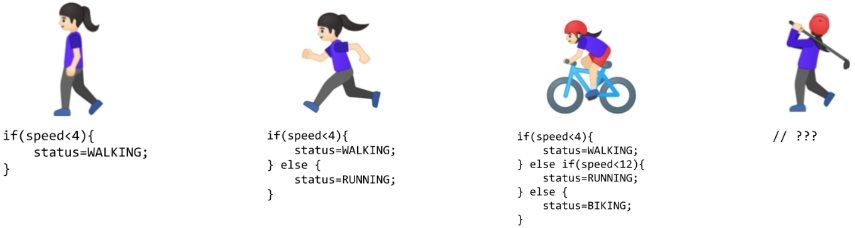
\end{tikzpicture}}Despite their apparent simplicity, rule-based limitations surface quickly with complex real-world tasks. Recognizing human activities illustrates the challenge. Classifying movement below 4 km/h as walking seems straightforward until real-world complexity intrudes. Speed variations, transitions between activities, and unanticipated cases each demand additional rules, as the successive code fragments in figure 4 show. Computer vision tasks compound these difficulties. Detecting cats requires rules about ears, whiskers, and body shapes while accounting for viewing angles, lighting, occlusions, and natural variations. Early systems achieved success only in controlled environments with well-defined constraints.
Recognizing these limitations, the knowledge engineering approach that characterized AI research in the 1970s and 1980s attempted to systematize rule creation. Expert systems5 encoded domain knowledge as explicit rules, showing promise in specific domains with well-defined parameters but struggling with tasks humans perform naturally: object recognition, speech understanding, and natural language interpretation. These failures highlighted a deeper challenge: many aspects of intelligent behavior rely on implicit knowledge that resists explicit rule-based representation.
5 Expert systems: These systems convert human expertise into explicit IF-THEN rules. This knowledge-engineering approach scales poorly for tasks such as object recognition, where the relevant variation is difficult to enumerate. Even successful systems such as DEC’s XCON accumulated thousands of hand-authored rules, making rule acquisition, consistency, and maintenance central engineering costs.
Consider one illustrative rule-based classifier for a 28 by 28 digit: compare pixel intensities against thresholds, check stroke patterns in specific regions, and branch on the results. Under this toy implementation, the computation is roughly 100 comparisons over 784 bytes of pixel data—small, predictable, and compatible with an ordinary CPU cache. The comparison establishes a workload baseline, not the accuracy of a production rule system.
The feature engineering bottleneck
The failures of rule-based systems suggested an alternative: rather than encoding human knowledge as explicit rules, let the system discover patterns from data. Machine learning offered this direction—instead of writing rules for every situation, researchers wrote programs that identified patterns in examples. The success of these methods, however, still depended heavily on human insight to define which patterns to look for, a process known as feature engineering.
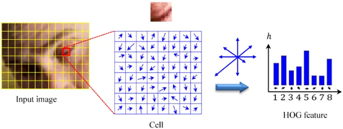
Feature engineering transformed raw data into representations that expose patterns to learning algorithms. The histogram of oriented gradients (HOG)6 (Dalal and Triggs 2005) method exemplifies this approach, identifying edges where brightness changes sharply, dividing images into cells, and measuring edge orientations within each cell (figure 5). This transforms raw pixels into shape descriptors robust to lighting variations and small positional changes.
6 Histogram of oriented gradients (HOG): An influential handcrafted descriptor for pedestrian detection before deep learning (Dalal and Triggs 2005). One common configuration computes gradient orientations in \(8{\times}8\) pixel cells, with cell size and other choices tuned for the task. HOG’s fixed computation graph can run efficiently on CPUs with predictable latency, while learned features can reduce descriptor redesign but do not automatically transfer across domains and often benefit from accelerators only as model and batch scale grow.
Dalal, Navneet, and Bill Triggs. 2005. “Histograms of Oriented Gradients for Human Detection.” 2005 IEEE Computer Society Conference on Computer Vision and Pattern Recognition (CVPR’05) 1: 886–93. https://doi.org/10.1109/cvpr.2005.177.
Bakheet, Samy, and Ayoub Al-Hamadi. 2021. “A Framework for Instantaneous Driver Drowsiness Detection Based on Improved HOG Features and Naïve Bayesian Classification.” Brain Sciences 11 (2): 240. https://doi.org/10.3390/brainsci11020240.
Complementary methods like scale-invariant feature transform (SIFT)7 (Lowe 1999) and Gabor filters8 captured different visual patterns. SIFT detected keypoints stable across scale and orientation changes, while Gabor filters identified textures and frequencies. Each encoded domain expertise about visual pattern recognition.
7 Scale-invariant feature transform (SIFT): SIFT encodes this domain expertise in a four-stage algorithm that identifies keypoints stable across scale and rotation. The number of detected keypoints varies by image, which complicates fixed-shape batching. Systems can regularize the representation through caps, padding, pooling, or fixed encodings, but each choice adds computation or discards information.
Lowe, David G. 1999. “Object Recognition from Local Scale-Invariant Features.” Proceedings of the Seventh IEEE International Conference on Computer Vision 2: 1150–1157 vol.2. https://doi.org/10.1109/iccv.1999.790410.
8 Gabor filters: Originally developed for localized time-frequency analysis (Gabor 1946), these filters detect edges and textures at specific orientations and frequencies. A typical bank contains many hand-designed filters across orientations and frequencies. Deep convolutional layers instead learn small kernels from data; early convolutional neural network (CNN) filters often become edge-, color-, and texture-sensitive detectors, shifting feature design from manual filter banks to data-driven optimization (Krizhevsky et al. 2012; LeCun et al. 2015).
Gabor, D. 1946. “Theory of Communication. Part 1: The Analysis of Information.” Journal of the Institution of Electrical Engineers - Part III: Radio and Communication Engineering 93 (26): 429–41. https://doi.org/10.1049/ji-3-2.1946.0074.
LeCun, Yann, Yoshua Bengio, and Geoffrey Hinton. 2015. “Deep Learning.” Nature 521 (7553): 436–44. https://doi.org/10.1038/nature14539.
These engineering efforts enabled advances in computer vision during the 2000s. Systems could now recognize objects with some robustness to real-world variations, leading to applications in face detection, pedestrian detection, and object recognition. Despite these successes, the approach had limitations. Experts needed to carefully design feature extractors for each new problem, and the resulting features might miss important patterns that were not anticipated in their design. The bottleneck remained: human expertise could not scale to the complexity and diversity of real-world visual patterns.
Return to the same 28 by 28 digit. In this illustrative implementation, HOG divides the image into a 7 by 7 grid of 4 by 4 cells, computes gradient magnitudes and orientations, bins them into 9 orientation histograms per cell, and produces a 441-element feature vector. A linear Support Vector Machine (SVM) classifier then performs ten dot products over that vector. The result is roughly 8,000 operations and about 2 KB of working memory—about 80× the work of the toy rule-based baseline, but still structured and well served by CPU vector units using single instruction, multiple data (SIMD). Descriptor size, class count, and implementation all change this cost.
Automatic pattern discovery
The limitations of handcrafted features motivate a more radical approach: rather than encoding features by hand, the system discovers its own. Neural networks embody exactly this shift—rather than following explicit rules or relying on human-designed feature extractors, the system learns representations directly from raw data.
Supervised learning changes the traditional programming relationship. Instead of encoding every decision rule directly, engineers provide examples and target answers, and optimization produces a learned model. Figure 6 makes this relationship tangible by showing learned rules as the output rather than the input. Humans still shape the task through data, objectives, architectures, and evaluation.
\resizebox{.65\textwidth}{!}{
\begin{tikzpicture}[font=\small\sffamily]
%
\tikzset{%
Line/.style={line width=1.0pt,black!50,text=black},
  Box/.style={inner xsep=2pt,
    node distance=1,
    draw=GreenLine, line width=0.75pt,
    fill=GreenL,
    text width=22mm,align=flush center,
    minimum width=22mm, minimum height=8mm
  },
  Box1/.style={Box,  draw=RedLine,
    fill=RedL, text width=36mm,
    minimum width=40mm
  },
}
%
 \node[Box1](B1){Machine Learning};
 \node[Box,right=of B1](B2){Rules};
 \node[Box,above left=0.2 and 1 of B1](B3){Answers};
 \node[Box, below left=0.2 and 1 of B1](B4){Data};
 \draw[-latex,Line](B1)--(B2);
 \draw[-latex,Line](B3)-|(B1);
 \draw[-latex,Line](B4)-|(B1);
\end{tikzpicture}}The system discovers patterns from examples through this automated process. When shown millions of images of cats, it learns to identify increasingly complex visual patterns, from simple edges to combinations that constitute cat-like features. This parallels how biological visual systems operate, building understanding from basic visual elements to complex objects.
The gradual layering of patterns reveals why neural network depth matters. For some compositional function classes, deeper networks can represent functions that require much wider shallow networks, an advantage formalized in section 1.2.1.
Deep learning often exhibits empirical scaling: within a given regime, performance can improve as additional data, compute, and model capacity are used effectively, although gains depend on data quality, optimization, architecture, and evaluation conditions. In the ImageNet competition, traditional methods achieved approximately 25.8 percent top-5 error in 2011. AlexNet9 reduced this to 15.3 percent in 2012. By 2015, ResNet achieved 3.6 percent top-5 error, lower than a published human baseline of approximately 5.1 percent under that evaluation protocol.
9 AlexNet’s memory split: Krizhevsky’s team split AlexNet across two NVIDIA GTX 580 GPUs, each with 3 GB of VRAM, so that the model and training state fit across the two devices. The workaround illustrates the systems lesson: a training configuration can exceed one device’s memory budget, forcing engineers to partition work and communication across devices.
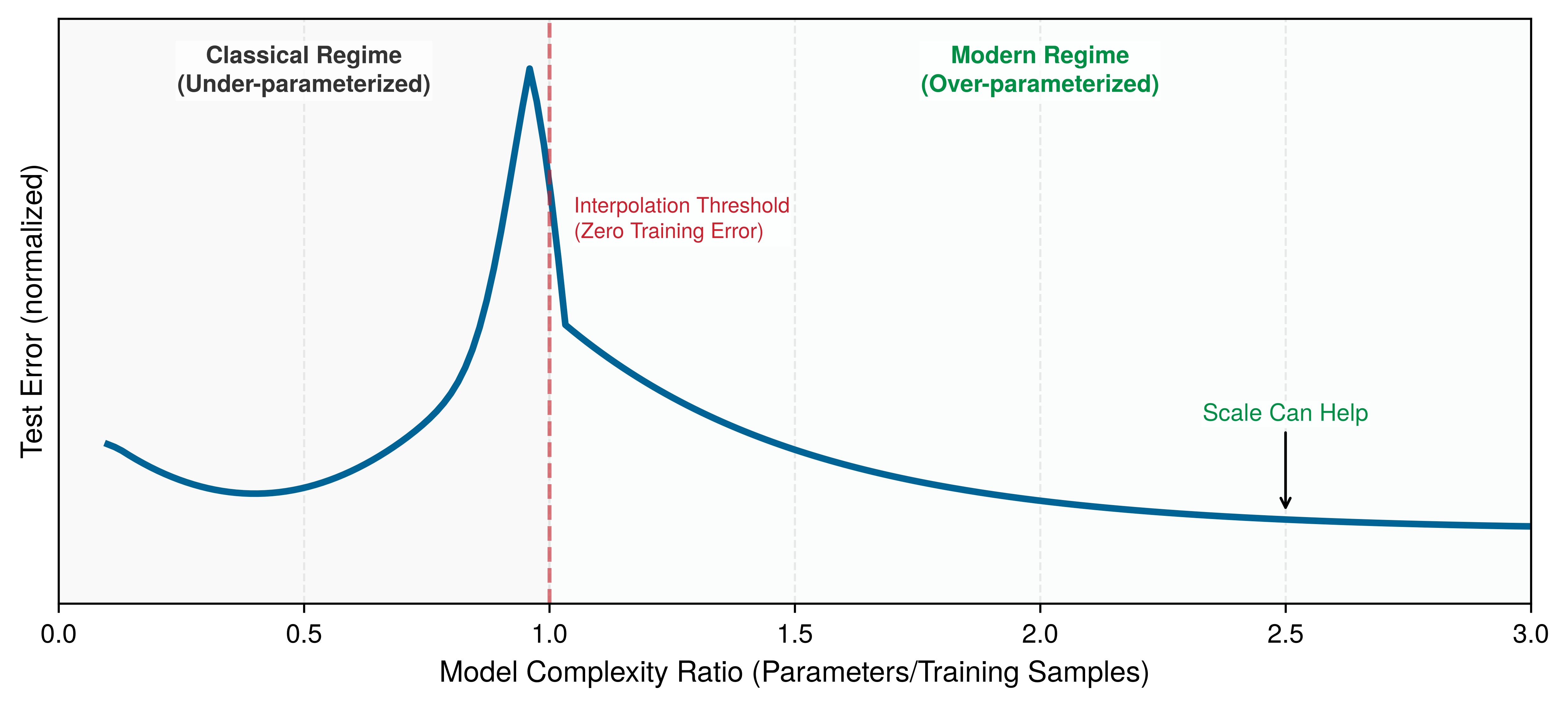
Figure 7 previews a phenomenon observed under some datasets, model families, and training procedures. The underlying mechanisms (training error, overfitting, gradient-based learning) are developed in subsequent sections; this section establishes the possible shape. The classical regime follows a U-shaped error curve, the interpolation threshold marks sufficient capacity to fit the training sample, and error can decrease again in an overparameterized regime. The axes are normalized to emphasize shape rather than a specific dataset.
The counterintuitive shape matters because test error, the error on held-out examples rather than the training examples the model sees directly, initially follows the expected U-curve, then decreases again when the model has more parameters than the simplest theory expects. This behavior complicates the classical account of overparameterization. The usual bias-variance trade-off10 suggests that models that are too small underfit, while models with excessive capacity risk fitting noise. Double descent (Belkin et al. 2019) shows that larger models can sometimes generalize better than smaller ones after the interpolation threshold. This overparameterization effect means that scale can be an engineering lever, not that scale is automatically safe: the data distribution, training procedure, and regularization still determine whether the extra capacity helps or memorizes. Overfitting and the regularization techniques that control it receive formal treatment in section 1.3.4.8; this preview needs only the shape of the curve.
10 Bias-variance trade-off: In some overparameterized regimes, test error decreases again after the interpolation threshold, so the classical single-U-shaped account is incomplete. The systems consequence is that model size cannot be treated as a universally monotonic overfitting risk. Larger models can become useful engineering options, provided the measured data, optimization, and regularization regime supports the gain.
Belkin, Mikhail, Daniel Hsu, Siyuan Ma, and Soumik Mandal. 2019. “Reconciling Modern Machine-Learning Practice and the Classical Bias–Variance Trade-Off.” Proceedings of the National Academy of Sciences 116 (32): 15849–54. https://doi.org/10.1073/pnas.1903070116.
Neural network performance follows empirical scaling relationships with direct systems consequences. The durable anchor is that frontier model sizes and training compute budgets have grown by orders of magnitude over the past decade (section 1.1.7 quantifies the trajectory). That growth makes arithmetic throughput, memory bandwidth, storage capacity, and communication potential bottlenecks whose importance depends on the workload and machine. Model Training develops the quantitative scaling formulations, including how model size, data, and compute trade off against one another; Model Compression explores the practical responses.
Neither relationship makes model size a decision rule. Double descent describes measured generalization under a particular data and training regime, while historical scaling describes resource investment across selected systems. Choosing a model still requires comparing candidates on representative deployment data and on the complete cost of training, serving, monitoring, and maintenance. The useful question is not whether additional scale can help, but whether its measured gain earns those system costs. That comparison should also include uncertainty in both gains and costs.
Systems Perspective 1.1: When to use neural networks
Not every problem benefits from deep learning. Neural networks are strong candidates when data exhibits spatial, sequential, or hierarchical structure that an architecture can exploit, simpler baselines miss the required task quality, and measured gains justify the complete system cost (table 1). With limited labels, low-dimensional tabular data, approximately linear relationships, hard latency limits, or strict auditability requirements, classical methods may match the useful performance of a neural network with less training, serving, and maintenance effort (table 2).
| Condition | Evidence to seek | Rationale |
|---|---|---|
| Representative data | Training and validation cover deployment conditions | Capacity cannot replace missing coverage |
| Exploitable structure | Spatial, sequential, or hierarchical patterns | Architecture can encode a useful prior |
| Baseline gap | Simpler methods miss the required task-quality target | Complexity buys a measured gain |
| Operational fit | Gain survives latency, memory, and cost limits | Offline accuracy alone is insufficient |
| Maintenance advantage | Learned features reduce recurring manual updates | Full-system maintenance becomes simpler |
| Condition | Baseline to test | Reason to prefer it |
|---|---|---|
| Limited labeled data | Linear model or tree ensemble | Lower variance and easier validation |
| Structured tabular inputs | Gradient boosting or linear model | Strong accuracy without learned features |
| Approximately linear signal | Linear or additive model | Transparent and inexpensive execution |
| Hard resource bound | Rules or compact classical model | Predictable latency, memory use, and energy demand |
| Direct auditability needed | Constrained tree or linear model | Decisions are easier to inspect |
Systems insight: Establish a simple baseline before building a neural network. Compare candidates on the task metric that matters and on the resources required to train, serve, monitor, and update them. Retain the neural approach only when its measured benefit justifies that added system. The document-recognition history in section 1.5 shows why the comparison must include preprocessing, rejection policy, and the cost of human review rather than model accuracy alone.
Learning representations from data reshapes AI system construction. Reducing manual feature engineering introduces new demands: infrastructure to handle large datasets, high-throughput hardware to process them, and specialized accelerators to perform mathematical calculations efficiently. These computational requirements have helped drive the development of chips optimized for neural network operations. Deep learning now underpins major systems in computer vision, speech recognition, game playing, and natural language processing.
Return to the same 28 by 28 digit, now processed by the chapter’s three-layer neural network (784 → 128 → 64 → 10). Under the stated implementations, the forward pass requires 109,184 MACs, 1,091.8× the work of the toy rule-based baseline. The 109,386 parameters consume 438 KB in 32-bit single-precision floating-point (FP32), exceeding most L1 caches and creating traffic between cache levels during inference. Training multiplies the cost further: each image is processed forward and backward before an update, with simplified dense-layer arithmetic on the order of three forward passes, repeated over 60,000 images for multiple epochs. Dense matrix multiplications now dominate this example’s arithmetic and favor parallel hardware. This workload change raises a practical question about when engineers should invest in neural networks rather than simpler alternatives.
Computational infrastructure requirements
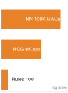
In this MNIST comparison, learned features spend far more arithmetic.
The MNIST running example traced one set of illustrative implementations from ~100 comparisons (rule-based) through ~8,000 operations (HOG) to 109,184 MACs (neural network): a 1,091.8× escalation in the stated operation models, with a corresponding shift toward parallel matrix operations. Table 3 summarizes the tendencies exposed by this comparison.
The comparison matters because each step changes the likely bottleneck: from branch-heavy CPU control, to batch-oriented feature pipelines, to memory-fed matrix parallelism. CPUs remain effective for small networks and latency-sensitive workloads, while large dense operations often map more efficiently to accelerators.
The shift toward parallelism creates new bottlenecks. The central challenge is the memory wall:11 compute throughput has grown faster than off-chip memory bandwidth. Whether a matrix operation is memory or compute bound depends on its arithmetic intensity: large, well-tiled matrix-matrix multiplication can be compute bound, whereas matrix-vector, small, skinny, or low-reuse layers are often limited by bandwidth.12 Hardware responses are examined in Understanding the AI memory wall, while The memory hierarchy details the memory hierarchy.
11 Memory wall: Fast on-chip storage responds in nanoseconds, while larger off-chip memory is orders of magnitude farther away in latency and energy. Neural network weights often exceed the smallest caches, so performance depends on tiling, larger cache levels, on-chip static RAM (SRAM), and high-bandwidth memory (HBM) to reuse values before another off-chip fetch. Insufficient reuse can leave compute units idle even when peak arithmetic throughput is high.
12 Memory-bound operations: Matrix multiplication’s arithmetic intensity (FLOP/byte loaded) determines whether a layer is compute bound or memory bound. Layers that fall below the hardware’s roofline crossover point finish their arithmetic before the next tile of weights arrives from memory. The result: effective hardware utilization can drop sharply, and adding more compute units yields little speedup until memory bandwidth or data reuse improves.
| System Aspect | Traditional Programming | ML with Features | Deep Learning |
|---|---|---|---|
| Computation | Often control-flow oriented | Structured parallel ops | Often matrix-parallel |
| Memory Access | Workload dependent | Commonly batch-oriented | Large tensor working sets |
| Data Movement | Program and input dependent | Feature-pipeline movement | Parameter and activation movement |
| Hardware Needs | Commonly CPU-centric | Often CPU with vector units | Frequently accelerator-friendly |
| Resource Scaling | Input and program dependent | Descriptor and data driven | Driven by width, batch, state, and reuse |
Energy adds a constraint alongside speed. Moving data from main memory to processing units can consume far more energy than a simple arithmetic operation (Horowitz 2014). This energy hierarchy explains why neural network accelerators maximize data reuse: they keep frequently accessed values in local storage and schedule operations to reduce movement. Whether movement or arithmetic dominates depends on precision, reuse, workload shape, and hardware, but the cost of movement motivates specialized architectures from data center GPUs to TinyML accelerators.
Horowitz, Mark. 2014. “1.1 Computing’s Energy Problem (and What We Can Do about It).” 2014 IEEE International Solid-State Circuits Conference Digest of Technical Papers (ISSCC), 10–14. https://doi.org/10.1109/isscc.2014.6757323.
The memory-computation trade-off manifests differently across the cloud-to-edge spectrum introduced in ML Systems. Cloud servers may use more memory and power to pursue throughput, while mobile devices operate within tighter power budgets. Large-batch training commonly emphasizes throughput; latency-sensitive or battery-powered inference may emphasize response time or energy per prediction. The exact priority depends on the deployment workload.
These single-machine constraints compound when scaling across multiple machines: dense layers scale with adjacent dimensions, batches scale activation storage and throughput demand, and training adds backward-pass, activation, and optimizer-state multipliers. Model-compression, hardware-acceleration, and training-system techniques all respond to this pressure by reducing the work, raising the useful machine rate, or changing where state lives.
The infrastructure demands traced earlier (parallelism, memory walls, and energy-dominated data movement) arise from how neural networks compute: weights that change during training, many simple units operating simultaneously, layers that compose low-level features into high-level concepts, and data reuse that minimizes energy-intensive movement. These properties manifest concretely in the fundamental building block of neural computation: the artificial neuron.13 Just as understanding a single transistor reveals how complex processors work, understanding the artificial neuron reveals how million-parameter networks operate.
13 Neuron: McCulloch and Pitts (1943) introduced a mathematical threshold model of nervous activity: inputs combine and an all-or-none output fires when a threshold is met. That logical neuron is an origin point for the artificial-neuron abstraction and for networks built from many simple units. Learned weights, deep hierarchies, and modern fused multiply-add (FMA) accelerator datapaths are later developments that turn this abstraction into the matrix-heavy workloads studied in this chapter.
McCulloch, Warren S., and Walter Pitts. 1943. “A Logical Calculus of the Ideas Immanent in Nervous Activity.” The Bulletin of Mathematical Biophysics 5 (4): 115–33. https://doi.org/10.1007/bf02478259.
The artificial neuron as a computing primitive
The basic unit of neural computation, the artificial neuron (or node), serves as a simplified mathematical abstraction of nervous activity (McCulloch and Pitts 1943). Later digital neural-network implementations adapted this abstraction into a standardized processing unit. This building block enables complex networks to emerge from simple components working together. Compare the biological and artificial neurons side by side in figure 8 to see how this computational model distills biological complexity into a simpler computational form.
\begin{tikzpicture}[line join=round,font=\sffamily\footnotesize]
\tikzset{
  Box/.style={,
    inner xsep=2pt,
    node distance=1.4,
    draw=GreenLine,
    line width=0.75pt,
    rounded corners,
    fill=mygreen!07,
    minimum width=65mm, minimum height=57mm
  },
    Txt/.style={black!50,font=\sffamily\itshape\fontsize {8pt}{7}\selectfont},
  }

\ExplSyntaxOn

\fp_new:N  \l__ctp_angle_fp
\tl_new:N  \l__ctp_spec_tl
\tl_new:N  \l__ctp_name_tl
\int_new:N \g__ctp_shading_int

\keys_define:nn { colour_transition_path }
  {
    angle .fp_set:N  = \l__ctp_angle_fp,
    angle .initial:n = 0,
  }

% Razdvaja stavku:
%   orange      -> boja=orange, pozicija prazna
%   orange/12   -> boja=orange, pozicija=12
\cs_new_protected:Npn \__ctp_split_item:nNN #1#2#3
  {
    \seq_set_split:Nnn \l_tmpa_seq {/} {#1}
    \tl_set:Ne #2 { \tl_trim_spaces:n { \seq_item:Nn \l_tmpa_seq {1} } }
    \int_compare:nNnTF { \seq_count:N \l_tmpa_seq } > {1}
      {
        \tl_set:Ne #3 { \tl_trim_spaces:n { \seq_item:Nn \l_tmpa_seq {2} } }
      }
      {
        \tl_clear:N #3
      }
  }

% Gradi shading specifikaciju.
% Ako pozicija nije data, računa se ravnomerno.
\cs_new_protected:Npn \__ctp_build_shading:n #1
  {
    \tl_clear:N \l__ctp_spec_tl

    \int_step_inline:nn { \clist_count:n {#1} }
      {
        \__ctp_split_item:nNN
          { \clist_item:nn {#1}{##1} }
          \l_tmpa_tl
          \l_tmpb_tl

        \tl_if_blank:VTF \l_tmpb_tl
          {
            \tl_set:Nx \l_tmpb_tl
              { \fp_eval:n { 100*(##1-1)/(\clist_count:n {#1}-1) } }
          }
          { }

        \tl_put_right:Nx \l__ctp_spec_tl
          {
            color(\tl_use:N \l_tmpb_tl bp)=(\tl_use:N \l_tmpa_tl)
          }

        \int_compare:nNnF {##1} = { \clist_count:n {#1} }
          {
            \tl_put_right:Nn \l__ctp_spec_tl { ; }
          }
      }
  }

\cs_new_protected:Npn \__ctp_declare_shading:
  {
    \int_gincr:N \g__ctp_shading_int
    \tl_set:Nx \l__ctp_name_tl
      { colourtransitionpath\int_use:N \g__ctp_shading_int }

    \use:e
      {
        \exp_not:N \pgfdeclarehorizontalshading
          { \tl_use:N \l__ctp_name_tl }
          { 100bp }
          { \tl_use:N \l__ctp_spec_tl }
      }
  }

% #1 = opcije (ugao)
% #2 = lista boja
% #3 = zatvorena putanja, BEZ završnog ;
\NewDocumentCommand \ColourTransitionPath { O{} m m }
  {
    \group_begin:
      \keys_set:nn { colour_transition_path } {#1}
      \clist_set:Nn \l_tmpa_clist {#2}

      \int_compare:nNnTF { \clist_count:N \l_tmpa_clist } = {1}
        {
          % Samo jedna boja
          \__ctp_split_item:nNN
            { \clist_item:Nn \l_tmpa_clist {1} }
            \l_tmpa_tl
            \l_tmpb_tl

          \path[fill=\l_tmpa_tl] #3 ;
        }
        {
          \__ctp_build_shading:n {#2}
          \__ctp_declare_shading:

          \path[
            path~picture={
              \shade[
                shading=\tl_use:N \l__ctp_name_tl,
                shading~angle=\fp_eval:n { -\l__ctp_angle_fp }
              ]
              (path~picture~bounding~box.north~west)
                rectangle
              (path~picture~bounding~box.south~east);
            }
          ] #3 ;
        }
    \group_end:
  }

\ExplSyntaxOff

\draw[black,fill=myorange](-0.81,0)to[out=200,in=330](-1.02,0)
to[out=-210,in=275](-1.13,0.23)to[out=90,in=225](-1.06,0.33)to[out=40,in=255](-0.99,0.43)
to[out=70,in=220](-0.8,0.79)to[out=200,in=70](-1.03,0.49)to[out=250,in=50](-1.11,0.37)
to[out=230,in=270](-1.15,0.4)to[out=100,in=250](-1.16,0.64)to[out=70,in=290](-1.12,1.13)
to[out=270,in=70](-1.205,0.68)to[out=240,in=310](-1.275,0.72)to[out=120,in=280](-1.41,1.07)
to[out=270,in=125](-1.28,0.62)to[out=310,in=100](-1.21,0.32)to[out=270,in=45](-1.26,0.08)
to[out=220,in=5](-1.50,0.0)to[out=175,in=260](-1.55,0.14)to[out=80,in=300](-1.6,0.38)
to[out=120,in=280](-1.73,0.78)to[out=260,in=120](-1.64,0.35)to[out=300,in=85](-1.615,0.09)
to[out=260,in=325](-1.73,0.095)to[out=149,in=315](-2.01,0.3)to[out=115,in=255](-1.967,0.48)
to[out=65,in=295](-1.959,0.77)to[out=265,in=285](-2.1,0.42)to[out=105,in=275](-2.205,0.87)
to[out=260,in=115](-2.14,0.39)to[out=295,in=135](-1.971,0.19)to[out=305,in=00](-2.1,0.166)
to[out=175,in=50](-2.43,0.04)to[out=25,in=170](-2.09,0.11)to[out=345,in=188](-1.91,0.09)
to[out=10,in=150](-1.71,0.02)to[out=-30,in=120](-1.58,-0.1)to[out=285,in=90](-1.57,-0.25)
to[out=280,in=60](-1.57,-0.45)to[out=240,in=20](-1.75,-0.58)to[out=180,in=320](-1.88,-0.48)
to[out=140,in=0](-2.29,-0.37)to[out=340,in=130](-1.85,-0.59)to[out=320,in=20](-1.95,-0.70)
to[out=200,in=90](-2.25,-1.20)to[out=70,in=230](-2.09,-0.87)to[out=45,in=200](-1.73,-0.69)
to[out=25,in=60](-1.68,-0.72)to[out=245,in=70](-1.79,-0.92)to[out=245,in=90](-1.84,-1.18)
to[out=75,in=220](-1.64,-0.83)to[out=55,in=190](-1.49,-0.59)to[out=5,in=120](-1.26,-0.69)
to[out=300,in=60](-1.26,-0.89)to[out=240,in=85](-1.36,-1.19)to[out=270,in=70](-1.42,-1.53)
to[out=40,in=90](-1.32,-1.17)to[out=88,in=230](-1.22,-0.93)to[out=68,in=110](-1.17,-0.93)
to[out=290,in=130](-1.08,-1.16)to[out=298,in=95](-1.06,-1.61)to[out=58,in=95](-1.00,-1.27)
to[out=115,in=125](-0.97,-1.2)to[out=335,in=135](-0.7,-1.36)to[out=95,in=340](-0.97,-1.15)
to[out=150,in=300](-1.06,-1.05)to[out=110,in=280](-1.155,-0.69)to[out=100,in=150](-0.99,-0.54)
to[out=325,in=170](-0.8,-0.62)to[out=-5,in=110](-0.755,-0.72)to[out=280,in=150](-0.455,-1.16)
to[out=130,in=280](-0.71,-0.70)to[out=105,in=180](-0.61,-0.655)to[out=355,in=160](-0.31,-0.73)
to[out=335,in=180](0.07,-0.84)to[out=155,in=330](-0.25,-0.70)to[out=145,in=230](-0.255,-0.643)
to[out=40,in=185](0.13,-0.54)to[out=170,in=45](-0.28,-0.61)to[out=220,in=340](-0.44,-0.62)
to[out=160,in=290](-0.95,-0.36)
to[out=105,in=190](-0.75,-0.11)coordinate(PL1)
to[out=5,in=190](0.10,-0.2)to[out=10,in=200](1.10,0.13)to[out=20,in=170](1.50,0.15)
to[out=345,in=152](1.88,0.01)to[out=325,in=122](1.95,-0.11)to[out=290,in=95](1.985,-0.30)
to[out=270,in=100](2,-0.60)
arc[start angle=110, end angle=430, radius=0.065] %1
to[out=95,in=280](2.031,-0.40)to[out=95,in=130](2.06,-0.395)to[out=305,in=150](2.288,-0.565)
arc[start angle=180, end angle=500, radius=0.065] %2
to[out=145,in=310](2.088,-0.35)to[out=135,in=280](2.03,-0.15)to[out=95,in=300](2.00,-0.06)
to[out=95,in=170](2.10,-0.06)to[out=95,in=170](2.10,-0.06)to[out=345,in=190](2.26,-0.06)
to[out=355,in=150](2.46,-0.21)to[out=320,in=150](2.55,-0.27)
arc[start angle=170, end angle=490, radius=0.065] %3
to[out=160,in=310](2.395,-0.09)to[out=130,in=180](2.42,-0.04)to[out=0,in=170](2.73,-0.03)
arc[start angle=170, end angle=490, radius=0.075] %4
to[out=170,in=10](2.4,0.01)to[out=190,in=350](2.1,0.03)to[out=170,in=330](1.91,0.07)
to[out=170,in=210](1.91,0.12)to[out=30,in=210](2.01,0.17)to[out=20,in=170](2.21,0.21)
to[out=330,in=180](2.41,0.18)to[out=10,in=170](2.52,0.185)
arc[start angle=180, end angle=495, radius=0.07] %5
to[out=190,in=350](2.28,0.23)to[out=160,in=190](2.28,0.28)to[out=35,in=210](2.48,0.41)
to[out=35,in=190](2.55,0.43)
arc[start angle=200, end angle=520, radius=0.07] %6
to[out=195,in=40](2.25,0.32)to[out=215,in=10](2.1,0.25)to[out=195,in=260](2.05,0.30)
to[out=70,in=230](2.185,0.50)
arc[start angle=250, end angle=565, radius=0.055] %7
to[out=215,in=75](1.99,0.25)to[out=255,in=25](1.93,0.2)to[out=205,in=25](1.83,0.161)
to[out=200,in=345](1.73,0.161)to[out=160,in=325](1.57,0.23)to[out=120,in=225](1.62,0.3)
to[out=40,in=235](1.76,0.45)to[out=50,in=215](1.96,0.60)to[out=45,in=210](2.33,0.79)
to[out=30,in=170](2.43,0.8)to[out=335,in=180](2.76,0.74)
arc[start angle=210, end angle=525, radius=0.06] %8
to[out=180,in=340](2.45,0.839)to[out=150,in=220](2.48,0.9)to[out=50,in=210](2.66,1.07)
arc[start angle=220, end angle=545, radius=0.065] %9
to[out=205,in=40](2.4,0.9)to[out=215,in=20](2.1,0.79)to[out=200,in=30](1.97,0.715)
to[out=220,in=250](1.925,0.75)to[out=90,in=245](1.975,0.95)to[out=65,in=225](2.175,1.15)
to[out=50,in=265](2.285,1.37)
arc[start angle=280, end angle=590, radius=0.05] %10
to[out=260,in=45](2.17,1.23)to[out=230,in=55](2.08,1.13)to[out=260,in=275](2.04,1.13)
to[out=100,in=255](2.034,1.44)
arc[start angle=285, end angle=590, radius=0.055] %11
to[out=260,in=105](1.98,1.15)to[out=280,in=55](1.92,0.95)to[out=230,in=90](1.85,0.67)
to[out=250,in=60](1.74,0.55)to[out=230,in=290](1.68,0.55)to[out=100,in=270](1.677,0.78)
to[out=100,in=290](1.65,0.86)to[out=72,in=260](1.767,1.08)to[out=72,in=270](1.78,1.18)
arc[start angle=295, end angle=600, radius=0.05] %12
to[out=272,in=60](1.64,0.95)to[out=252,in=280](1.6,0.95)to[out=112,in=270](1.545,1.25)
arc[start angle=290, end angle=610, radius=0.07] %13
to[out=260,in=100](1.58,0.82)to[out=150,in=300](1.274,1.1)
arc[start angle=320, end angle=620, radius=0.05] %14
to[out=300,in=140](1.35,0.92)to[out=320,in=130](1.55,0.75)to[out=320,in=90](1.58,0.59)
to[out=290,in=50](1.58,0.394)to[out=230,in=0](1.34,0.27)to[out=180,in=20](1.0,0.23)
to[out=200,in=30](0.5,0.03)to[out=210,in=180](-0.05,-0.07)
to[out=180,in=340](-0.45,0.01)to[out=166,in=10]cycle;

\definecolor{col1}{RGB}{131,216,255}
\definecolor{col2}{RGB}{65,167,250}
\definecolor{col3}{RGB}{36,110,173}
\definecolor{col4}{RGB}{0,18,34}
\definecolor{col5}{RGB}{14,60,102}
\definecolor{col6}{RGB}{32,112,180}

\ColourTransitionPath[angle=100]
    {col5,col4,col5,col5,col1,col1,col1}
    {
      (-0.6,0.12)
      to[out=5,in=170](-0.17,0.04)
      to[out=290,in=70](-0.23,-0.29)
      to[out=180,in=330](-0.65,-0.17)
      to[out=90,in=240]cycle
    }

\draw[black](-0.6,0.12)coordinate(1X1)
to[out=5,in=170](-0.17,0.04)
to[out=290,in=70](-0.23,-0.29)coordinate(1X2)
to[out=180,in=330](-0.65,-0.17)
to[out=90,in=240]cycle;

\coordinate(1S1)at($(1X1)!0.5!(1X2)$);
\node[draw=none,ellipse,minimum width=2mm,minimum height=1.2mm,
inner sep=0pt,rotate=-10,fill=col3](EL1)at(1S1){};
\node[draw=none,ellipse,minimum width=1.75mm,minimum height=0.8mm,
inner sep=0pt,rotate=-10,fill=col2,anchor=south]at(EL1.south){};
\node[draw=none,ellipse,minimum width=1.5mm,minimum height=0.4mm,
inner sep=0pt,rotate=-10,fill=col1,anchor=south]at(EL1.south){};
\node[draw=black,ellipse,minimum width=2mm,minimum height=1.2mm,
inner sep=0pt,rotate=-10,fill=none](EL1)at(1S1){};

%the second
\ColourTransitionPath[angle=80]
    {col5,col4,col5,col5,col1,col1,col1}
    {
    (-0.09,0.04)
to[out=0,in=190](0.3,0.09)
to[out=300,in=85](0.39,-0.25)
to[out=200,in=350](-0.09,-0.29)
to[out=97,in=260]cycle;
    }

\draw[black](-0.09,0.04)coordinate(2X1)
to[out=0,in=190](0.3,0.09)
to[out=300,in=85](0.39,-0.25)coordinate(2X2)
to[out=200,in=350](-0.09,-0.29)
to[out=97,in=260]cycle;

\coordinate(2S1)at($(2X1)!0.5!(2X2)$);
\node[draw=none,ellipse,minimum width=2mm,minimum height=1.2mm,
inner sep=0pt,rotate=10,fill=col3](EL2)at(2S1){};
\node[draw=none,ellipse,minimum width=1.75mm,minimum height=0.8mm,
inner sep=0pt,rotate=10,fill=col2,anchor=south]at(EL2.south){};
\node[draw=none,ellipse,minimum width=1.5mm,minimum height=0.4mm,
inner sep=0pt,rotate=10,fill=col1,anchor=south]at(EL2.south){};
\node[draw=black,ellipse,minimum width=2mm,minimum height=1.2mm,
inner sep=0pt,rotate=10,fill=none]at(2S1){};

%The third
\ColourTransitionPath[angle=65]
    {col5,col4,col5,col5,col1,col1,col1}
    {
(0.38,0.1)
to[out=25,in=190](0.76,0.27)
to[out=298,in=95](0.86,-0.04)
to[out=210,in=5](0.48,-0.2)
to[out=117,in=280]cycle;
    }

\draw[black](0.38,0.1)coordinate(3X1)
to[out=25,in=190](0.76,0.27)
to[out=298,in=95](0.86,-0.04)coordinate(3X2)
to[out=210,in=5](0.48,-0.2)
to[out=117,in=280]cycle;

\coordinate(3S1)at($(3X1)!0.5!(3X2)$);
\node[draw=none,ellipse,minimum width=2mm,minimum height=1.2mm,
inner sep=0pt,rotate=25,fill=col3](EL3)at(3S1){};
\node[draw=none,ellipse,minimum width=1.75mm,minimum height=0.8mm,
inner sep=0pt,rotate=25,fill=col2,anchor=south]at(EL3.south){};
\node[draw=none,ellipse,minimum width=1.5mm,minimum height=0.4mm,
inner sep=0pt,rotate=25,fill=col1,anchor=south]at(EL3.south){};
\node[draw=black,ellipse,minimum width=2mm,minimum height=1.2mm,
inner sep=0pt,rotate=25,fill=none]at(3S1){};

%The fourth
\ColourTransitionPath[angle=65]
    {col5,col4,col5,col5,col1,col1,col1}
    {
(0.84,0.285)
to[out=25,in=190](1.26,0.39)
to[out=298,in=95](1.32,0.08)
to[out=185,in=5](0.93,-0.02)
to[out=117,in=280]cycle;
    }

\draw[black](0.84,0.285)coordinate(4X1)
to[out=25,in=190](1.26,0.39)
to[out=298,in=95](1.32,0.08)coordinate(4X2)
to[out=185,in=5](0.93,-0.02)
to[out=117,in=280]cycle;

\coordinate(4S1)at($(4X1)!0.5!(4X2)$);
\node[draw=none,ellipse,minimum width=2mm,minimum height=1.2mm,
inner sep=0pt,rotate=15,fill=col3](EL4)at(4S1){};
\node[draw=none,ellipse,minimum width=1.75mm,minimum height=0.8mm,
inner sep=0pt,rotate=15,fill=col2,anchor=south]at(EL4.south){};
\node[draw=none,ellipse,minimum width=1.5mm,minimum height=0.4mm,
inner sep=0pt,rotate=15,fill=col1,anchor=south]at(EL4.south){};
\node[draw=black,ellipse,minimum width=2mm,minimum height=1.2mm,
inner sep=0pt,rotate=15,fill=none]at(4S1){};

%left

\coordinate(0S1)at(-1.25,-0.26);
\node[draw=none,ellipse,minimum width=3.8mm,minimum height=2.8mm,
inner sep=0pt,rotate=0,fill=col3](EL0)at(0S1){};
\node[draw=none,ellipse,minimum width=3.5mm,minimum height=1.9mm,
inner sep=0pt,rotate=0,fill=col2,anchor=south]at(EL0.south){};
\node[draw=none,ellipse,minimum width=3.1mm,minimum height=1.2mm,
inner sep=0pt,rotate=0,fill=col1,anchor=south]at(EL0.south){};
\node[draw=black,ellipse,minimum width=3.8mm,minimum height=2.8mm,
inner sep=0pt,rotate=0,fill=none]at(0S1){};

\coordinate (P1) at (2.00,-0.60);
\coordinate (N1) at ($(P1)-({0.065*cos(110)},{0.065*sin(110)})$);

\coordinate (P2) at (2.288,-0.565);
\coordinate (N2) at ($(P2)-({0.065*cos(180)},{0.065*sin(180)})$);

\coordinate (P3) at (2.55,-0.27);
\coordinate (N3) at ($(P3)-({0.065*cos(170)},{0.065*sin(170)})$);

\coordinate (P4) at (2.73,-0.03);
\coordinate (N4) at ($(P4)-({0.075*cos(170)},{0.075*sin(170)})$);

\coordinate (P5) at (2.52,0.185);
\coordinate (N5) at ($(P5)-({0.07*cos(180)},{0.07*sin(180)})$);

\coordinate (P6) at(2.55,0.43);
\coordinate (N6) at ($(P6)-({0.07*cos(200)},{0.07*sin(200)})$);

\coordinate (P7) at(2.185,0.5);
\coordinate (N7) at ($(P7)-({0.055*cos(250)},{0.055*sin(250)})$);

\coordinate (P8) at(2.76,0.74);
\coordinate (N8) at ($(P8)-({0.06*cos(210)},{0.06*sin(210)})$);

\coordinate (P9) at(2.66,1.07);
\coordinate (N9) at ($(P9)-({0.065*cos(220)},{0.065*sin(220)})$);

\coordinate (P10) at(2.285,1.37);
\coordinate (N10) at ($(P10)-({0.05*cos(280)},{0.05*sin(280)})$);

\coordinate (P11) at(2.034,1.44);
\coordinate (N11) at ($(P11)-({0.055*cos(285)},{0.055*sin(285)})$);

\coordinate (P12) at(1.78,1.18);
\coordinate (N12) at ($(P12)-({0.05*cos(295)},{0.05*sin(295)})$);

\coordinate (P13) at(1.545,1.25);
\coordinate (N13) at ($(P13)-({0.07*cos(290)},{0.07*sin(290)})$);

\coordinate (P14) at(1.274,1.1);
\coordinate (N14) at ($(P14)-({0.05*cos(320)},{0.05*sin(320)})$);

\foreach \x / \v in {1/1.64pt,2/1.64pt,3/1.64pt,
4/1.94pt,5/1.85pt,6/1.85pt,7/1.4pt,8/1.5pt,9/1.65pt,
10/1.3pt,11/1.4pt,12/1.3pt,13/1.8pt,14/1.3pt
}{
\shade[ball color=cyan!50!blue] (N\x) circle (\v);
}
%Labeling
\draw[](0S1)--++(245:1.65)node[below]{Nucleus};
\draw[](0S1)+(300:0.2)--++(306:1.65)node[below]{\textbf{Cell Body}};
\node[]at(-0.15,0.99){\textbf{Dendrites}};
\draw[red,<-,>=Latex](-2.1,0.9)--++(80:0.65)node[above=0pt,inner sep=0pt]{\textbf{Inputs}};
\node[]at(0.9,-0.4){\textbf{Axon}};
\draw[red,<-,>=Latex](N3)+(270:0.14)--++(256:1.15)node[below]{\textbf{Outputs}};

\begin{scope}[on background layer]
\node[Box](BB1)at(0.25,-0.1){};
\node[Box,right=2.5 of BB1](BB2){};
\end{scope}
\node[below=9pt of BB1.north,GreenLine]{\textbf{Biological Neuron}};
\node[below=9pt of BB2.north,GreenLine]{\textbf{Artificial Neuron}};

\begin{scope}[shift={($(BB2)+(-2.15,1.4)$)}]
 \tikzset{%
  Line/.style={line width=1.0pt,black!50,text=black},
  Box2/.style={inner sep=2pt,
    node distance=0.23,circle,
    draw=VioletLine, line width=0.75pt,
    fill=VioletL2,
    align=flush center,
    minimum width=8mm,
  },
}
%
\node[Box2](B1){$x_{0}$};
\node[Box2,below=of B1](B2){$x_1$};
\node[Box2,below=of B2](B3){$x_2$};
\node[Box2,node distance=0.7,below=of B3](B4){$x_n$};
\node[rotate=90,font=\tiny\sffamily]at($(B3)!0.5!(B4)$){$\bullet$ $\bullet$ $\bullet$};

\node[above=0.1 of B1,font=\sffamily\small](WE){\textbf{Inputs}};
\node[Box2,minimum width=12mm,right=2of $(B1)!0.5!(B4)$,
            fill=VioletL2,draw=VioletLine](B5){};
\draw[VioletLine,dashed,thick](B5.north)--(B5.south);
\node[right=2pt of B5.west]{\textbf{z}};
\node[left=2pt of B5.east]{\textbf{f}};
%
\node[below left=0 and -0.5 of B5.south,align=left]{Linear\\Function};
\node[below right=0 and 0.5 of B5.south,align=left]{Activation\\Function};
\foreach \x in{1,...,4}{
\draw[Line](B\x)--coordinate[pos=0.4](S\x)(B5);
}
\node[right=0pt of B1]{$=1$};
\node[below=0pt of S1]{$b$};
\node[below=0pt of S2]{$w_1$};
\node[below=0pt of S3]{$w_2$};
\node[below=3pt of S4]{$w_n$};
%
\draw[Line,-latex](B5)--node[above,pos=0.8]{$y$}++(1.97,0)
node[below,pos=0.7]{\textbf{Output}};
\end{scope}
%%between
\coordinate(TG)at($(BB1.north east)!0.5!(BB2.north west)$);
\coordinate(TD)at($(BB1.south east)!0.5!(BB2.south west)$);

\draw[black!40,shorten >=4mm,shorten <=4mm](TG)--(TD);

\foreach \x[count =\a]  in {0.14,0.38,0.62,0.85}{
\fill[black!30]($(TG)!\x!(TD)$) circle(2pt)coordinate(Q\a);
}
\node[above=2pt of Q1,Txt]{Dendrites};
\node[below=2pt of Q1,Txt]{= Inputs};

\node[above=2pt of Q2,Txt]{Synapses};
\node[below=2pt of Q2,Txt]{= Weights};

\node[above=2pt of Q3,Txt]{Soma};
\node[below=2pt of Q3,Txt]{= Linear fn(z)};

\node[above=2pt of Q4,Txt]{Axon firing};
\node[below=2pt of Q4,Txt]{= Activation (f)};

\end{tikzpicture}The right panel of figure 8 traces the signal through four stages, each translating a biological structure into a mathematical operation:
- Input Reception (Dendrites → \(x_1, x_2, \dots, x_n\)): The artificial neuron receives a vector of input features \(\mathbf{x}\). In MNIST digit recognition, these represent pixel intensities. The dendrite analogy captures reception of many signals without claiming biological equivalence.
- Weighted Modulation (Synapses → \(w_1, w_2, \dots, w_n\)): Each input is multiplied by a learnable weight \(w_i\), just as synaptic strengths modulate biological signals. These weights act as “gain” controls, determining how much influence each feature has on the final decision. A bias term \(b\) (shown as the top input \(x_0 = 1\) in figure 8) shifts the activation threshold. Across a network, learned behavior is distributed over many such parameters rather than stored in one weight.
- Signal Aggregation (Cell Body → Linear Function \(z\)): The neuron integrates the weighted signals, producing a single scalar value \(z = \sum (x_i \cdot w_i) + b\). This mirrors how a biological cell body sums incoming electrochemical signals to determine whether the neuron has received enough evidence for a particular pattern.
- Nonlinear Activation (Axon → Activation Function \(f\)): The aggregated signal passes through an activation function \(f(z)\), producing the output \(y\). This mirrors the axon’s all-or-nothing firing decision: the nonlinearity determines whether the neuron “fires” a signal to the next layer. Unlike the biological case, \(f\) can produce graded outputs (for example, ReLU passes positive values through, zeroes negatives), but the principle is the same—thresholding followed by propagation. Table 4 formalizes these correspondences.
| Biological Structure | Artificial Component | Mathematical Operation | Engineering Role |
|---|---|---|---|
| Dendrites (receive signals) | Input Vector | \(\mathbf{x} = [x_1, \dots, x_n]\) | Data ingestion from sensors or prior layers |
| Synapses (modulate strength) | Weight Vector | \(\mathbf{w} = [w_1, \dots, w_n]\) | Learnable parameters encoding importance |
| Cell Body (integrates signals) | Linear Function \(z\) | \(z = \sum (x_i \cdot w_i) + b\) | Linear integration of feature signals |
| Axon (fires output) | Activation Function \(f\) | \(a = f(z)\) | Nonlinear thresholding and signal propagation |
From a systems engineering perspective, this translation reveals why neural networks can have demanding computational requirements. A direct scalar evaluation of one neuron performs \(N\) multiply-accumulate (MAC)14 operations and, without reuse, loads \(N\) inputs, \(N\) weights, and a bias before writing the output. Batched and tiled kernels reuse inputs and weights across many neuron evaluations, reducing traffic per MAC. At network scale, performance therefore depends on both the number of operations and how effectively the implementation reuses data.
14 MAC (multiply-accumulate): A core operation in dense and convolutional layers is \(a \leftarrow a + (b \times c)\). Hardware data sheets often report fused multiply-add throughput in FLOPs because one multiply and one add count as two floating-point operations. On that convention, the reported FLOP/s rate is twice the MAC/s rate when a MAC is counted as one multiply-accumulate. Layer and batch choices also create activation, communication, and data-movement costs, so MAC count is necessary but not sufficient for a systems budget.
The transition from individual neurons to integrated systems requires navigating the central trade-off between representational capacity and computational cost. Digital hardware performs arithmetic quickly, but the volume of operations and data movement in deep networks creates bottlenecks that a single-neuron view does not expose.
Replicating intelligent behavior in silicon confronts three interrelated system-level constraints. As models grow, moving parameters and activations can become more limiting than arithmetic throughput. Concurrency clashes with dependency: many operations inside a layer can run in parallel, but layer \(\ell+1\) still depends on layer \(\ell\), placing a lower bound on end-to-end latency. Precision also trades against memory, throughput, and energy: wider representations consume more storage and data movement, while narrower formats require evidence that task quality remains acceptable. Model Compression develops this search for minimum viable precision.
Addressing these constraints requires two complementary strategies. An architectural inductive bias is a built-in structural assumption about the data: convolutional networks assume nearby pixels matter together in images, while recurrent networks assume order matters in sequences. Encoding those assumptions restricts the function class toward structures expected to be useful (Mitchell 1980). Computational scaling supplies additional capacity and optimization effort. Modern AI engineering combines both approaches, using architectural structure to make effective use of available scale.
Mitchell, Tom M. 1980. The Need for Biases in Learning Generalizations. CBM-TR-117. Rutgers University, Department of Computer Science.
Hardware and software requirements
Translating neural concepts to silicon carries a physical cost. Feature extraction can become weighted linear sums followed by nonlinear activations, while dense interactions become matrix operations that hardware must execute efficiently. The mathematical graph, however, does not prescribe an execution plan. Frameworks and compilers must choose kernels, tensor layouts, fusion boundaries, and schedules for a particular processor. Two implementations can therefore compute the same function with the same nominal arithmetic count yet differ substantially in data traffic, temporary storage, and latency. Hardware supplies arithmetic units, memory, and communication links; software determines how the graph uses them. This translation layer decides whether the parallelism visible in the model becomes useful machine utilization.
A neural network’s learned behavior is distributed across parameters stored at ordinary memory addresses. Inference fetches parameters and activations; training adds saved intermediates, gradients, and optimizer state, so storage capacity and bandwidth both matter. Biological synapses combine storage and local processing, whereas digital accelerators move values through a memory hierarchy. The brain consumes about 20 percent of the body’s resting oxygen and calories (Raichle and Gusnard 2002), although direct efficiency comparisons are misleading because biological and artificial systems perform different tasks under different accuracy and latency constraints. The narrower systems lesson is that data movement matters enough to motivate the specialized hardware in Hardware Acceleration and the optimization strategies in Model Compression.
Raichle, Marcus E., and Debra A. Gusnard. 2002. “Appraising the Brain’s Energy Budget.” Proceedings of the National Academy of Sciences 99 (16): 10237–39. https://doi.org/10.1073/pnas.172399499.
These hardware demands did not emerge overnight. The tension between algorithmic ambition and available silicon has shaped the entire trajectory of neural network research, from the earliest perceptrons to today’s trillion-parameter models.
Evolution of neural network computing
The perceptron15 introduced a probabilistic neuron model for learning and information storage (Rosenblatt 1958). Its simple mathematics met a hardware constraint: larger networks needed far more processing and memory. Deep learning evolved through this algorithm-silicon co-evolution; the neuron abstraction remained recognizable while the hardware able to execute it transformed. That co-evolution frames the history that follows: progress required both better methods and better machines.
15 Perceptron: A machine built to execute a learning algorithm, directly linking hardware and software from the start. A single linear-threshold layer cannot represent nonlinearly separable functions such as XOR, regardless of additional input hardware. Multilayer nonlinear networks expand the representable function class, but they also introduce the training and systems costs developed in this chapter.
Rosenblatt, Frank. 1958. “The Perceptron: A Probabilistic Model for Information Storage and Organization in the Brain.” Psychological Review 65 (6): 386–408. https://doi.org/10.1037/h0042519.
16 Backpropagation: Short for “backward propagation of errors,” the algorithm uses the chain rule to compute how the loss is locally sensitive to millions of weights. It does not establish which weights historically caused an error. Werbos applied it to neural networks in 1974 (Werbos 1974), and the 1986 Rumelhart, Hinton, and Williams publication demonstrated practical effectiveness (Rumelhart et al. 1986). The systems cost: backprop requires storing forward-pass activations and additional training state, creating the several-times-higher memory footprint quantified later in the chapter.
The backpropagation16 algorithm was applied to neural networks by Paul Werbos in his 1974 PhD thesis (Werbos 1974), building on Seppo Linnainmaa’s 1970 work on automatic differentiation (Linnainmaa 1970), and was later popularized by Rumelhart, Hinton, and Williams (Rumelhart et al. 1986). Their publication demonstrated the algorithm’s practical effectiveness and brought it to widespread attention in the machine learning community, triggering renewed interest in neural networks. This chapter returns to the algorithm in section 1.3.4; Backpropagation mechanics develops its systems-level implementation. The 1986 demonstration showed that hidden units could learn useful internal features, but it did not resolve the systems problem of scaling training. Larger models multiply forward operations, saved activations, gradient computations, and parameter updates. Practical adoption therefore depended on improvements across the complete stack rather than on the learning rule alone.
This history yields a recurring systems lesson: an algorithm becomes useful only when the complete system can train and evaluate it effectively. The lag between early backpropagation work17 and widespread adoption reflected the maturation of hardware, data, initialization, nonlinearities, optimization, benchmarks, and software infrastructure. An algorithm can therefore be viable in principle long before its surrounding system makes it useful in practice. Deep learning came from this convergence, not from a new mathematical discovery alone.
17 Algorithm-system adoption lag: Backpropagation was available in neural-network form by 1974 (Werbos 1974), while the 1986 Rumelhart, Hinton, and Williams demonstration brought it much wider attention (Rumelhart et al. 1986). Attention mechanisms appeared in neural machine translation in 2014, transformers made them central in 2017, and later TPU- and GPU-scale infrastructure enabled much larger deployments. These histories do not imply that every computationally expensive idea will succeed. They show that an algorithm should be evaluated together with the data, optimization methods, software, hardware, and task regime needed to make it useful.
Werbos, Paul. 1974. “Beyond Regression: New Tools for Prediction and Analysis in the Behavioral Sciences.” PhD thesis, Harvard University.
Rumelhart, David E., Geoffrey E. Hinton, and Ronald J. Williams. 1986. “Learning Representations by Back-Propagating Errors.” Nature 323 (6088): 533–36. https://doi.org/10.1038/323533a0.
The term itself gained prominence in the 2010s, coinciding with advances in computational power and data accessibility. The scale of this computational explosion is difficult to grasp without visualization. Figure 9 plots representative estimates of AI training compute across nearly seven decades on a logarithmic scale, revealing two fitted regimes: total training compute, measured in floating-point operations (FLOPs), followed a comparatively slow pre-2010 trend, then the post-2012 deep-learning frontier accelerated sharply. Large-scale models after 2015 sit orders of magnitude above the pre-2010 trajectory, showing that modern progress reinvests hardware and algorithmic gains into much larger training runs.
Beyond raw compute, this growth carries an energy cost that systems engineers cannot ignore. Under the stated scenario assumptions, a three-day LeNet-1 workstation run would use roughly 54 kWh. Applying an external GPT-4 GPU-day estimate and a data-center-overhead factor yields about 33,600 MWh, comparable to the annual electricity use of roughly 3,200 representative US homes.18 These are order-of-magnitude estimates, not measured utility records, and they vary with accelerator utilization, facility overhead, and the calculation boundary. Even so, the scale makes energy per operation and achieved utilization design concerns alongside peak FLOP/s. The quantitative energy analysis appears in Hardware Acceleration.
18 Training energy scale: The estimate assumes a 750 W workstation for the historical run and uses 10.5 MWh/year as a representative US household electricity budget. The closed-model scenario treats an external GPU-day estimate as A100-equivalent accelerator time and applies a simple data-center overhead. The result illustrates scale; it does not establish the actual energy used to train GPT-4.
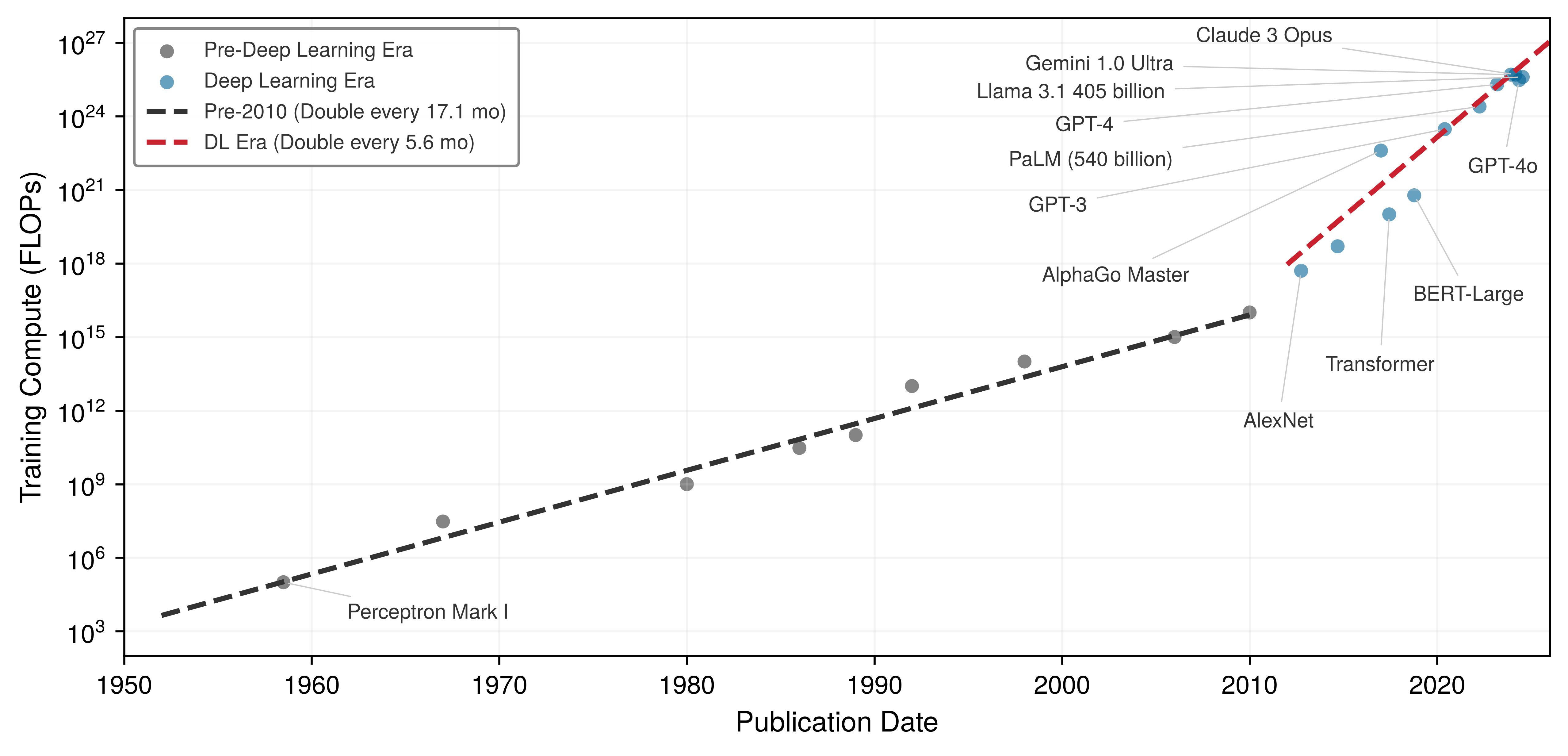
Table 5 grounds these trends in representative systems, showing how parameters, compute, and hardware co-evolved across four decades of neural network development. Three patterns deserve separate treatment. First, the plotted post-2012 training-compute frontier rises on a timescale of months, although the fitted rate depends on the selected systems and on uncertain estimates. Second, algorithmic and systems advances have reduced the compute needed to reach fixed benchmark targets in some domains, so a frontier-compute trend does not describe efficiency at a constant capability. Third, hardware utilization, reduced precision, software maturity, and procurement conditions mediate the relationship between raw compute and monetary cost; they do not guarantee that cost grows more slowly. For systems engineers, these distinctions affect infrastructure timelines, experimental budgets, and build-versus-buy decisions. Planning therefore requires measured efficiency, a stated comparison target, and explicit uncertainty, especially for closed models whose architecture and training configuration are undisclosed.
| Year | System | Params | Train FLOPs | Hardware | Train Time | Error/Task |
|---|---|---|---|---|---|---|
| 1989 | LeNet-1 | ~10K | \(10^{11}\)–\(10^{12}\) | Sun-4/260 workstation | 3 days | 1% at 12.1% rejection (USPS digits) |
| 1998 | LeNet-5 | \(60\text{K} \pm 1\text{K}\) | \(10^{14} \pm 1\text{ OoM}\) | SGI Origin 2000 (200 MHz) | 2–3 days | 0.95% (MNIST) |
| 2012 | AlexNet | ~60M | \(5 \times 10^{17}\) | 2\(\times\) GTX 580 GPUs | 5–6 days | 15.3% (ImageNet) |
| 2015 | ResNet-152 | ~60M | \(10^{19} \pm 0.5\text{ OoM}\) | 8\(\times\) Tesla K80 GPUs | ~3 weeks | 3.6% (ImageNet) |
| 2020 | GPT-3 | 175B (exact) | \(3 \times 10^{23}\) | Undisclosed | Undisclosed | N/A (language) |
| 2023 | GPT-4 | Undisclosed | \(10^{24}\)–\(10^{25}\) (external est.) | Undisclosed | Undisclosed | N/A (language) |
Advances across three dimensions reinforced these trends: data availability, algorithmic innovations, and computing infrastructure. Follow the arrows in figure 10 to see the interaction: faster infrastructure made larger data and models practical, growing datasets created new opportunities and pressures for algorithms, and algorithmic advances changed the demands placed on computing systems. The cycle is enabling rather than automatic: progress in one dimension can expose a bottleneck in another rather than produce an immediate gain.
\begin{tikzpicture}[font=\small\sffamily]

\tikzset{
    Box/.style={draw=none,minimum width=44mm, minimum height=25mm, node distance=16mm},
    Arr/.style={-{Triangle[width=10pt,length=8pt]}, line width=5pt,cyan!40,shorten >=1pt, shorten <=2pt},
 Box2/.style={align=flush center, inner xsep=2pt,draw=none,
  font=\footnotesize\sffamily\bfseries, line width=0.75pt, fill=OrangeL!30, text width=38mm,
    minimum width=44mm, minimum height=7mm},
  Box3/.style = {Box2,draw=none,fill=cyan!10},
  Box4/.style = {Box2,draw=none,fill=GreenFill!60},
LineA/.style = {violet!60,{Circle[line width=1.0pt,fill=white,length=5.5pt]}-,line width=1.5pt,shorten <=-3pt},
    Arr/.style={-{Triangle[width=9pt,length=11pt]}, line width=3pt,mybrown!30,shorten >=1pt, shorten <=2pt},
Txt/.style = {font=\footnotesize\sffamily,black!80,align=center}
}

%cloud ML
\tikzset {
pics/cloudA/.style = {
        code = {
        \pgfkeys{/channel/.cd, #1}
\begin{scope}[local bounding box=CLO,scale=\scalefac, every node/.append style={transform shape}]
\node[draw=\drawcolor!90!red,line width=\Linewidth,minimum width=6mm,minimum height=12mm](VSK)at(0,0.5){};
\node[draw=\drawcolor!90!red,line width=\Linewidth,fill=white,minimum width=9mm,minimum height=4mm](VSKG)at(VSK.north){};
\node[draw=\drawcolor!90!red,line width=\Linewidth,fill=white,minimum width=9mm,minimum height=4mm](VSKC)at(VSK.center){};
\node[draw=\drawcolor!90!red,line width=\Linewidth,fill=white,minimum width=9mm,minimum height=4mm](VSKD)at(VSK.south){};
\draw[fill=\filllcolor,draw=\drawcolor!60,,line width=\Linewidth](0,0)to[out=170,in=180,distance=11](0.1,0.61)
to[out=90,in=105,distance=17](1.07,0.71)
to[out=20,in=75,distance=7](1.48,0.36)
to[out=350,in=0,distance=7](1.48,0)--(0,0);
\draw[draw=\drawcolor!60,,line width=\Linewidth](0.27,0.71)to[bend left=25](0.49,0.96);
\draw[draw=\drawcolor!60,,line width=\Linewidth](0.67,1.21)to[out=55,in=90,distance=13](1.5,0.96)
to[out=360,in=30,distance=9](1.68,0.42);
\node[single arrow, draw=orange,fill=orange,
      minimum width = 10pt, single arrow head extend=3pt,
      minimum height=10mm,
      rotate=270]at(1.05,0) {};
\end{scope}
}
}
}
    % #1 number of teeths
    % #2 radius intern
    % #3 radius extern
    % #4 angle from start to end of the first arc
    % #5 angle to decale the second arc from the first
    % #6 inner radius to cut off
    \tikzset{
      pics/gear/.style args={#1/#2/#3/#4/#5/#6/#7}{
       code={
               \pgfkeys{/channel/.cd, #7}
    \begin{scope}[shift={($(0,0)+(0,0)$)},scale=\scalefac,every node/.append style={transform shape}]
        \pgfmathtruncatemacro{\N}{#1}%
        \def\rin{#2}\def\rout{#3}\def\aA{#4}\def\aOff{#5}\def\rcut{#6}%
        \path[rounded corners=1.5pt,draw=\drawcolor,fill=\filllcolor]
          (0:\rin)
          \foreach \i [evaluate=\i as \n using (\i-1)*360/\N] in {1,...,\N}{%
            arc (\n:\n+\aA:\rin)
            -- (\n+\aA+\aOff:\rout)
            arc (\n+\aA+\aOff:\n+360/\N-\aOff:\rout)
            -- (\n+360/\N:\rin)
          } -- cycle;
          \draw[draw=none,fill=white](0,0) circle[radius=\rcut];
    \end{scope}
      }}
    }

\tikzset {
pics/cloudML/.style = {
        code = {
        \pgfkeys{/channel/.cd, #1}
\begin{scope}[local bounding box=CLO,scale=\scalefac, every node/.append style={transform shape}]
\draw[fill=\filllcolor,draw=\drawcolor!60,,line width=\Linewidth](0,0)to[out=170,in=180,distance=11](0.1,0.61)
to[out=90,in=105,distance=17](1.07,0.71)
to[out=20,in=75,distance=7](1.48,0.36)
to[out=350,in=0,distance=7](1.48,0)--(0,0);
\draw[draw=\drawcolor!60,,line width=\Linewidth](0.27,0.71)to[bend left=25](0.49,0.96);
 \draw[red,rounded corners,line width=\Linewidth,-{Circle[red,fill=yellow,length=6.5pt]}]
(0.3,0.1)--++(0,-8mm)--++(-5mm,0);
 \draw[violet,rounded corners,line width=\Linewidth,-{Circle[violet,fill=yellow,length=6.5pt]}]
(0.7,0.1)--++(0,-10mm);
 \draw[blue,rounded corners,line width=\Linewidth,-{Circle[blue,fill=yellow,length=6.5pt]}]
(1.1,0.1)--++(0,-8mm)--++(5mm,0);
\pic[shift={(0,0)}] at (0.65,0.1) {gear={12/1.5/1.9/8/4/0.8/scalefac=0.35,
drawcolor=mypurple,filllcolor=mypurple}};
\end{scope}
}
}
}
\tikzset {
pics/mobile/.style = {
        code = {
        \pgfkeys{/channel/.cd, #1}
\begin{scope}[local bounding box=MOB,scale=\scalefac, every node/.append style={transform shape}]
\node[rectangle,draw=\drawcolor,minimum height=94,minimum width=47,
            rounded corners=4,thick,fill=white](R1){};
\node[rectangle,draw=\drawcolor,minimum height=67,minimum width=38,thick,fill=\filllcolor](R2){\Large AI};
\node[circle,minimum size=8,below= 2pt of R2,inner sep=0pt,thick,fill=\filllcirclecolor]{};
\node[rectangle,fill=\filllcirclecolor,minimum height=1,minimum width=20,above= 4pt of R2,inner sep=0pt,thick]{};
%
 \end{scope}
     }
  }
}

\tikzset{mycylinder/.style={cylinder, shape border rotate=90, aspect=1.3, draw, fill=white,
minimum width=25mm,minimum height=11mm,line width=\Linewidth,node distance=-0.15},
pics/dataP/.style = {
        code = {
        \pgfkeys{/channel/.cd, #1}
\begin{scope}[local bounding box=STREAMING,scale=\scalefac, every node/.append style={transform shape}]
\node[mycylinder,fill=\filllcolor!50] (A) {};
\node[mycylinder, above=of A,fill=\filllcolor!50] (B) {};
\node[mycylinder, above=of B,fill=\filllcolor!10] (C) {};
\fill[\filllcolor!50!black]($(C.west)!0.12!(C.east)$)circle(3pt);
\fill[\filllcolor!50!black]($(B.west)!0.12!(B.east)$)circle(3pt);
\fill[\filllcolor!50!black]($(A.west)!0.12!(A.east)$)circle(3pt);
%
\draw[draw=\drawcolor,line width=2.5*\Linewidth](B.east)--++(17mm,0);
\node[draw=\drawcolor,line width=\Linewidth,minimum width=9mm,fill=white,minimum height=22mm](BD)at($(B.east)+(8mm,0)$){};
\node[draw=\drawcolor,line width=\Linewidth,minimum width=5mm,minimum height=8mm,fill=white](BDM)at($(BD.east)+(5mm,0)$){};
\node[circle,draw=orange,line width=\Linewidth,minimum size=5mm]at($(BD.north)!0.2!(BD.south)$){};
\node[rectangle,draw=blue,line width=\Linewidth,minimum size=5mm]at($(BD.north)!0.5!(BD.south)$){};
\node[circle,draw=green,line width=\Linewidth,minimum size=5mm]at($(BD.north)!0.8!(BD.south)$){};
\end{scope}
     }
  }
}
%nodes
\tikzset{
pics/nodes/.style = {
        code = {
        \pgfkeys{/channel/.cd, #1}
\begin{scope}[scale=\scalefac,every node/.append style={transform shape}]
\node[draw=white,fill=none,circle,minimum size=0.925*40mm,line width=1pt](CI){};
\draw[step=5mm,draw=white] (-2,-2) grid (2,2);
\foreach \x/\y[count=\a] in {-0.2/0.35,
0.7/0.6,-0.5/1.4,-1.20/-0.8,-0.1/-1.3,-0.4/-0.43,
0.61/-0.3,1/-0.85,0.45/1.2,-0.96/0.63}{
\node[circle,fill=myblue,draw=black,inner sep=0pt,minimum size=3mm](XB\a)at(\x,\y){};
}
\foreach \x/\y[count=\a] in {-2.0/0.1
}{
\node[circle,fill=myred,draw=black,inner sep=0pt,minimum size=3mm](XR\a)at(\x,\y){};
}
\foreach \x/\y[count=\a] in {1.87/0.1
}{
\node[circle,fill=mygreen,draw=black,inner sep=0pt,minimum size=3mm](XG\a)at(\x,\y){};
}
\foreach \x in {1,3,4,6,10}{
\draw[RedLine,line width=0.5pt](XR1) edge  (XB\x);
}
\foreach \x in {1,2,5,8,9}{
\draw[mygreen,line width=0.5pt](XG1) edge  (XB\x);
}
\foreach \x in {2,3,6,9,10}{
\draw[black,line width=0.5pt](XB1) edge  (XB\x);
}
\foreach \x in {4,5,7}{
\draw[black,line width=0.5pt](XB6) edge  (XB\x);
}
\draw[black,line width=0.5pt](XB4) edge  (XB5);
\draw[black,line width=0.5pt](XB3) edge  (XB9);
\foreach \x in {2,8}{
\draw[black,line width=0.5pt](XB7) edge  (XB\x);
}
\end{scope}
    }
  }
}
\tikzset {
pics/infras/.style = {
        code = {
        \pgfkeys{/channel/.cd, #1}
\begin{scope}[local bounding box=CLO,scale=\scalefac, every node/.append style={transform shape}]
\draw[fill=\filllcolor,draw=\drawcolor!60,,line width=\Linewidth](0,0)to[out=170,in=180,distance=11](0.1,0.61)
to[out=90,in=105,distance=17](1.07,0.71)
to[out=20,in=75,distance=7](1.48,0.36)
to[out=350,in=0,distance=7](1.48,0)--(0,0);
\draw[draw=\drawcolor!60,,line width=\Linewidth](0.27,0.71)to[bend left=25](0.49,0.96);
%
\node[draw=black,fill=mygreen!30,line width=\Linewidth,minimum width=7mm,minimum height=6mm](VSK)at(0.7,0.1){};
\node[draw=black,fill=myblue!20,line width=\Linewidth,minimum width=4mm,minimum height=3mm](VSK0)at(0.7,0.1){};
\node[draw=black,fill=mypurple!30,line width=\Linewidth,minimum width=6mm,minimum height=5mm,
below=4.5mm of VSK](VSK1){};
\node[draw=black,fill=myorange!30,line width=\Linewidth,minimum width=6mm,minimum height=5mm,
right=3.0mm of VSK1](VSK2){};
\node[draw=black,fill=myred!40,line width=\Linewidth,minimum width=6mm,minimum height=5mm,
left=3.0mm of VSK1](VSK3){};
\draw[black,shorten >=-2pt,-{Circle[fill=white,length=5.5pt]},
line width=\Linewidth,rounded corners](VSK.240)--++(0,-2mm)-| (VSK3.center);
\draw[black,shorten >=-2pt,-{Circle[fill=white,length=5.5pt]},
line width=\Linewidth,rounded corners](VSK.300)--++(0,-2mm)-| (VSK2.center);
\draw[black,shorten >=-2pt,-{Circle[fill=white,length=5.5pt]},
line width=\Linewidth,rounded corners](VSK.270)-- (VSK1.center);
\end{scope}
}
}
}
\pgfkeys{
  /channel/.cd,
   Depth/.store in=\Depth,
  Height/.store in=\Height,
  Width/.store in=\Width,
  filllcirclecolor/.store in=\filllcirclecolor,
  filllcolor/.store in=\filllcolor,
  drawcolor/.store in=\drawcolor,
  drawcircle/.store in=\drawcircle,
  scalefac/.store in=\scalefac,
  Linewidth/.store in=\Linewidth,
  picname/.store in=\picname,
  filllcolor=BrownLine,
  filllcirclecolor=violet!20,
  drawcolor=black,
  drawcircle=violet,
  scalefac=1,
  Linewidth=0.5pt,
  Depth=1.3,
  Height=0.8,
  Width=1.1,
  picname=C
}
%Data Available
\node[Box, fill=white](B1){};
\pic[shift={(-0.56,-0.6)}] at  (B1){dataP={scalefac=0.56,picname=1,filllcirclecolor=violet!20,filllcolor=myorange, Linewidth=0.7pt}};
\draw[violet,line width=1.5pt](B1.south west)--coordinate(S1)(B1.south east);
\node[Box3,anchor=north,below= 0.2 of B1](T1){Data Availability};
%Algorithmic Innovations
\node[Box, right=of B1](B2){};
 \pic[shift={(0,0)}] at  (B2){nodes={scalefac=0.75,drawcolor=orange,filllcirclecolor=orange!20,filllcolor=orange}};
\draw[violet,line width=1.5pt](B2.south west)--coordinate(S2)(B2.south east);
\node[Box3,anchor=north,below= 0.2 of B2](T2){Algorithmic Innovations};
%Computing Infrastructure
\node[Box, right=of B2](B3){};
\pic[shift={(-0.70,0.1)}] at  (B3){infras={scalefac=1.0,filllcirclecolor=orange!80,drawcolor=BlueLine,
filllcolor=cyan!10,  Linewidth=1.0pt}};
\draw[violet,line width=1.5pt](B3.south west)--coordinate(S3)(B3.south east);
\node[Box3,anchor=north,below= 0.2 of B3](T3){Computing Infrastructure};
%
\draw[Arr](T3)--++(0,-12mm)coordinate(DO)-|(T1);
\begin{scope}[on background layer]
\node[draw=myorange,inner sep=3mm,dashed,line width=1pt,fit=(T1)(B1)(B3)(DO)](F1){};
\node[myorange,anchor=south east,font=\small\sffamily\bfseries]at(F1.north east){Key Breakthroughs};
\end{scope}
%
\draw[Arr](B1)--(B2);
\draw[Arr](B2)--(B3);
\end{tikzpicture}Data availability supplied the volume of examples that learned representations require. The rise of the internet and digital devices created vast new sources of training data: image sharing platforms provided millions of labeled images, digital text collections enabled language processing at scale, and sensor networks generated continuous streams of real-world data. This abundance provided the raw material neural networks needed to learn complex patterns effectively.

Neural-network history is a scale explosion in training energy.
Algorithmic innovations turned that volume into trainable systems. New methods for initializing networks and controlling learning rates made training more stable. Techniques for controlling overfitting improved generalization in measured regimes. Researchers also documented empirical relationships among model size, computation, data quantity, and performance, leading to increasingly ambitious architectures while leaving the useful scaling regime task dependent.
Checkpoint 1.1: Understanding deep learning's emergence
Before connecting this history to its infrastructure consequences, verify your understanding of why deep learning emerged:
If any of these concepts remain unclear, review the relevant sections before continuing. The systems consequences that follow build directly on this conceptual foundation.
The resulting workloads created demand for higher-throughput computing infrastructure, which evolved in response. On the hardware side, GPUs provided the parallel processing capabilities needed for efficient neural network computation, and Tensor Processing Units (TPUs)19 (Jouppi et al. 2023) pushed performance further. High-bandwidth memory systems and fast interconnects addressed data movement challenges. Software advances matched the hardware evolution: frameworks and libraries simplified building and training networks, distributed computing systems enabled training at scale, and tools for optimizing model deployment reduced the gap between research and production.
19 TPU (tensor processing unit): Google’s custom accelerator, first deployed internally in 2015, was optimized specifically for the matrix multiplications that dominate neural network workloads. The TPU v1 achieved 92 TOPS (vendor-reported INT8 tera-operations/s) for inference at 75 W, a power-efficiency point that general-purpose GPUs of the era could not match. The name “Tensor Processing Unit” reflects the design decision to sacrifice general-purpose flexibility for maximum throughput on the operation neural networks need most.
Jouppi, Norm, George Kurian, Sheng Li, Peter Ma, Rahul Nagarajan, Lifeng Nai, Nishant Patil, et al. 2023. “TPU v4: An Optically Reconfigurable Supercomputer for Machine Learning with Hardware Support for Embeddings.” Proceedings of the 50th Annual International Symposium on Computer Architecture, 1–14. https://doi.org/10.1145/3579371.3589350.
The convergence of data availability, algorithmic innovation, and computational infrastructure created the foundation for modern deep learning. The preceding checkpoint consolidates this arc before the chapter returns to the computational operations that drive it.
The historical trajectory from perceptrons through periods of reduced interest to GPU-era deep learning reveals a recurring systems pattern: an algorithm may exist before data, optimization, software, benchmarks, and hardware make it practical. Modern frontier models again press against memory and energy budgets. Understanding the mathematical operations that create those pressures requires examining the computational primitives themselves.
Self-Check: Question
A team replaces a hand-coded digit recognition system (\(\approx 100\) conditional comparisons, \(784\text{ bytes}\) of working state) with a \(784 \to 128 \to 64 \to 10\) MLP (\(\approx 109{,}184\text{ MACs}\), \(\approx 438\text{ KB}\) of weights) on the same MNIST input. Which systems consequence should they expect when deploying this new model on a commodity CPU?
- The workload becomes dominated by branch mispredictions because artificial neurons execute frequent if-then branching decisions.
- The workload transitions from branch-heavy scalar code to dense matrix arithmetic whose weight footprint exceeds L1 cache capacity, generating cache-level memory traffic absent in the rule-based system.
- Execution memory traffic drops to zero because the \(438\text{ KB}\) weight footprint fits entirely within standard CPU register files.
- The model executes without using arithmetic logic units (ALUs) because learned representations bypass hardware compute pipelines.
A hardware vendor claims that increasing single-threaded CPU clock frequencies by \(5\times\) will eliminate the necessity of specialized accelerators (such as GPUs or TPUs) for deep neural networks. Based on the computational profile of neural networks, what is the strongest technical refutation of this claim?
- Deep learning is dominated by massive parallel matrix multiplications bounded by arithmetic throughput and memory bandwidth, which benefit from thousands of parallel SIMD/tensor units rather than higher scalar clock speeds.
- Higher CPU clock frequencies force the loss function to become non-convex, destabilizing gradient descent.
- Modern neural networks require asynchronous analog circuits that cannot be simulated on digital CPU cores.
- Increasing CPU clock frequencies reduces the numerical precision of floating-point registers to 4-bit integers.
A computer vision team evaluates two approaches for a multi-class recognition task: (a) a handcrafted feature pipeline (e.g. HOG + SVM) and (b) an end-to-end convolutional neural network. Compare the systems engineering trade-offs between these two approaches when the product must scale from 2 initial categories to 50 diverse object categories.
Explain the systems-level concept of the ‘algorithm-hardware adoption lag’ using the historical trajectory of backpropagation (Werbos 1974 / Rumelhart et al. 1986) and modern deep learning. What three converging factors were necessary for the algorithm to achieve widespread practical viability?
True or False: The artificial neuron is an exact biological model that reproduces the electrochemical ion channels and temporal spike-timing dynamics of human cortical neurons in digital silicon.
Order the historical evolution of pattern-computing paradigms and milestones from earliest to latest: (1) Deep learning with automatic hierarchical feature discovery on parallel accelerators, (2) Rule-based programming with explicit hand-authored logical branches, (3) The Rosenblatt single-layer Perceptron, (4) Classical machine learning pairing hand-engineered feature extractors (e.g. HOG/SIFT) with statistical classifiers.
Neural Network Fundamentals
The question now is why the computational demands can become so extreme. For suitable neural workloads, a GPU can outperform a CPU because it provides high parallel throughput and data reuse for matrix and tensor operations, not simply because of clock speed. The structure of these network primitives—neurons, layers, and nonlinear activations—determines how data flows through hardware and how memory demands scale during training and inference. Understanding these operations reveals how simple arithmetic on individual neurons compounds into the infrastructure requirements that shaped modern AI.
The concepts here apply to the feed-forward neural networks that anchor this chapter and recur in many larger architectures. Their common fundamentals are weighted sums, nonlinear activations, and gradient-based learning. Mastering these operations and their computational characteristics provides a basis for reasoning about more specialized networks, while later chapters introduce operators and execution patterns that this simple model does not contain.
Why depth matters: The power of hierarchical representations
A single-layer network attempting to classify handwritten digits must map raw pixels directly to labels. A deeper network can instead exploit hierarchical structure when the target function is compositional. The question is why depth can provide such representational advantages, and the answer grounds all the mathematical development that follows.
Deep networks can exploit compositionality: complex patterns may decompose into simpler patterns that themselves decompose further. In image recognition, learned representations can progress from local edges and textures toward parts and objects. Such hierarchical regularities occur in many datasets and motivate layered models, although a trained network need not recover this exact sequence.
Consider recognizing the digit “seven” in the MNIST example. A single-layer network maps all 784 pixel values directly to a decision. When the task has compositional structure, a deep network can compute the decision more parameter-efficiently by reusing intermediate features:
- Layer 1 learns simple edge detectors: vertical lines, horizontal lines, diagonal strokes
- Layer 2 combines edges into shapes: the horizontal top stroke of a “seven,” the diagonal downstroke
- Layer 3 combines shapes into complete digit patterns
Each layer builds on the previous, allowing later computations to reuse earlier features. This hierarchy can be much more parameter-efficient than a shallow representation when the task has suitable compositional structure. The same edge detectors learned for “seven” can also contribute to recognizing “one,” “four,” and other digits. This parameter reuse helps explain why depth is an effective design choice without implying a fixed parameter advantage for every task. However, the choice between adding layers and widening existing ones is not symmetric: depth and width contribute to representational capacity through different mechanisms.
Layered processing in biological vision helped motivate hierarchical models, without implying that artificial networks reproduce the same mechanisms. The architectures examined in Network Architectures encode different structural assumptions for images, sequences, and other data types. Depth explains why layered representations can be useful; the remaining mechanics explain how the hierarchy is implemented. The following sections develop those mechanics: how neurons compute, how layers connect, and how information flows from input to output.
Systems Perspective 1.2: The depth vs. width trade-off
For certain function classes, depth provides an exponential representational advantage: a network with \(N_L\) layers can represent functions that require exponentially more units in a shallow network (Telgarsky 2016). This restricted theoretical result explains why nonlinear composition can be parameter-efficient; it is not a universal guarantee for every task.
However, depth introduces three engineering challenges with each additional layer:
- Adds sequential dependencies (layer \(\ell+1\) waits for layer \(\ell\)), limiting parallelism
- Increases gradient path length, risking vanishing/exploding gradients
- Requires storing intermediate activations for backpropagation
Modern architectures balance depth against width. A network with ten layers of 100 neurons has the same 1,000 total hidden units as one with two layers of 500, but not the same parameter count, function class, or execution graph. Both expose parallelism within each layer; the deeper network adds sequential dependencies and may represent some compositional functions more efficiently.
Telgarsky, Matus. 2016. “Benefits of Depth in Neural Networks.” Proceedings of the 29th Annual Conference on Learning Theory, 1517–39.
Network architecture fundamentals
A neural network’s architecture determines how information flows from input to output. Modern networks can be enormously complex, but they all build on a few organizational principles that shape both implementation and the computational infrastructure they demand.
Handwritten digit recognition grounds these concepts in a concrete example, specifically the task of classifying images from the MNIST dataset (LeCun et al. 1998). This seemingly simple task reveals all the core principles of neural networks while providing intuition for more complex applications.
Each architectural choice, from how neurons are connected to how layers are organized, creates specific computational patterns that must be efficiently mapped to hardware. This mapping between network architecture and computational requirements is essential for building scalable ML systems.
Example 1.1: Running example: MNIST digit recognition
Scenario: Deploying a basic handwritten digit classifier on \(28{\times}28\) grayscale images across 10 output classes.
Diagnosis: The chapter’s running architecture maps 784 raw pixel features through 128 and 64 hidden units to 10 outputs, creating roughly 100K parameters.
Systems lesson: Inspecting input vector dimensions and layer parameters on a compact dataset establishes baseline compute and memory bandwidth requirements before scaling to high-dimensional production workloads.
The perceptron’s weighted sum
The computational machinery within each dense layer is a perceptron-style artificial neuron whose signal path (inputs, weights, bias, aggregation, activation) section 1.1.5 traced through its biological origins. What remains is to formalize that path mathematically, because this repeated operation becomes the layer-level kernel that hardware executes. In the MNIST network, a first-layer unit combines all 784 pixel intensities into one activation that may respond to a learned pattern, such as a vertical edge shared by “one” and “seven.” Follow figure 11 from left to right: each input \(x_i\) is multiplied by its corresponding weight \(w_{ij}\), the products are accumulated with a bias, and an activation function transforms the resulting score. Different neurons repeat the same structure with different learned weights, allowing one layer to test many patterns against the same input.
\scalebox{0.85}{
\begin{tikzpicture}[font=\sffamily]
\tikzset{%
  Line/.style={line width=1.0pt,black!50,text=black},
  Box/.style={inner xsep=3pt,
    node distance=0.4,
    circle,
    draw=GreenLine, line width=0.75pt,
    fill=GreenL,
    align=flush center,
    minimum width=8mm,
  },
}
%
\node[Box](B1){$w_{1j}$};
\node[Box,below=of B1](B2){$w_{2j}$};
\node[Box,below=of B2](B3){$w_{3j}$};
\node[Box,node distance=1.0,below=of B3](B4){$w_{ij}$};
\node[rotate=90,font=\tiny\sffamily]at($(B3)!0.5!(B4)$){$\bullet$ $\bullet$ $\bullet$};
\foreach \x in{1,...,3}{
\draw[Line,latex-](B\x)--++(180:2)node[left](X\x){$x_\x$};
}
\node[above=0.1 of B1,font=\sffamily\small](WE){Weights};
\path[](WE)-|coordinate(IN)(X1);
\node[font=\sffamily\small]at(IN){Inputs};

\draw[Line,latex-](B4)--++(180:2)node[left](X4){$x_i$};
\node[rotate=90,font=\tiny\sffamily]at($(X3)!0.5!(X4)$){$\bullet$ $\bullet$ $\bullet$};
\node[Box,minimum width=12mm,right=2of $(B1)!0.5!(B4)$,
            fill=RedL,draw=RedLine](B5){$\sum$};
\foreach \x in{1,...,4}{
\draw[Line,-latex](B\x)--(B5);
}
%
\node[Box,node distance=1.3,rectangle, right=of B5,fill=BlueL,
            draw=BlueLine, minimum width=11mm, minimum height=11mm,
            font=\sffamily\huge](SI){$\sigma$};
\draw[Line,-latex](B5)--node[above]{$z$}(SI);
\draw[Line,latex-,font=\sffamily\small](B5)--
           node[right]{$b$}++(270:1.75)node[below,]{Bias};
\draw[Line,-latex](SI)--++(0:1.75)node[right](OU){$\hat{y}$};
\node[above=0.1 of OU,font=\sffamily\small]{Output};
\node[below=0.3 of SI,font=\sffamily\small,align=center]{Activation\\ function};
\end{tikzpicture}}Each input \(x_i\) has a corresponding weight \(w_{ij}\), and the perceptron multiplies each input by its matching weight. The intermediate output, \(z\), is computed as the weighted sum of inputs in equation 1: \[ z = \sum (x_i \cdot w_{ij}) \tag{1}\]
Here, \(j\) identifies the receiving neuron once perceptrons are assembled into a layer, and the sum runs over all input indices \(i\). In plain terms, each input feature is scaled by how important it is (its weight), and the results are summed into a single score. This is the dot product of two vectors—the fundamental operation that hardware accelerators are designed to execute at maximum throughput, and the reason neural network performance is measured by the number of MAC operations completed per second.
A bias term \(b\) shifts the linear output up or down, giving the model additional flexibility to fit the data. Thus, the intermediate linear combination computed by the perceptron including the bias becomes equation 2: \[ z = \sum (x_i \cdot w_{ij}) + b \tag{2}\]
With this weighted sum in hand, a suitable output activation and loss can support regression or classification. A binary linear-threshold classifier selects one of two classes around a threshold; multiclass networks instead produce several scores and commonly normalize them with softmax.
Under the direct scalar, no-reuse accounting established earlier, one neuron performs \(N\) multiply-accumulate operations and moves its inputs, weights, bias, and output. What the formalization adds is the layer view. A dense layer of \(M\) neurons repeats the weighted sum \(M\) times, so its arithmetic cost is \(M \times N\) MACs—exactly the matrix multiplication \(\mathbf{x}\mathbf{W}\) that hardware must execute, and the form in which the rest of this chapter counts work.
Nonlinear activation functions
Activation functions are where expressiveness, gradient flow, and hardware cost meet. They convert linear weighted sums into nonlinear outputs; without them, multiple linear layers would collapse into a single linear transformation, severely limiting the network’s expressive power. Figure 12 compares three commonly used element-wise activation functions and one vector-level function (softmax), each with mathematical characteristics that shape both learning behavior and execution cost.
\begin{tikzpicture}[line join=round,font=\sffamily\small]
\pgfplotsset{
    compat=1.15,
    MyStyle/.style={
        title style={yshift=-1mm},
        legend style={at={(0.17,0.88)}, anchor=south},
        legend cell align={left},
        axis x line=bottom,
        axis y line*=left,
        axis line style={thick},
        width=10cm,
        height=7cm,
        grid = major,
        major grid style={dashed},
        xlabel = {},
        tick style = {line width=1.0pt},
        tick align = inside,
        tick label style={/pgf/number format/assume math mode=true},
        ticklabel style={font=\footnotesize\sffamily,
},
   yticklabel style={ font=\footnotesize\sffamily,
  /pgf/number format/fixed,
  /pgf/number format/fixed zerofill,
  /pgf/number format/precision=2
},
    },
}

 \begin{scope}[local bounding box=GR1,shift={($(0,0)+(0,0)$)}]
 \begin{axis}[
        title = {Sigmoid Activation Function},
        MyStyle,
        ymin=-0.05, ymax=1.05,
        xmin=-10.5,xmax=10.75,
        xtick={-10.0,-7.5,-5,0,-2.5,0.0,2.5,5.0,7.5,10.0},]
        \addplot[
BlueLine,line width=2pt,
            domain = -10:10,
            samples = 100
        ]
            {1/(1+exp(-x))};
            \addlegendentry{Sigmoid}
    \end{axis}
    \end{scope}
 %
\begin{scope}[local bounding box=GR2,shift={($(0,0)+(10.5,0)$)}]
 \begin{axis}[
        title = {Tanh Activation Function},
        MyStyle,
        ymin=-1.1, ymax=1.1,
        xmin=-10.5,xmax=10.75,
        xtick={-10.0,-7.5,-5,0,-2.5,0.0,2.5,5.0,7.5,10.0},
        ytick={-1.00,-0.75,-0.5,-0.25,0.0,0.25,0.50,0.75,1.00},
    ]
        \addplot[
            OrangeLine,line width=2pt,
            domain = -10:10,
            samples = 100
        ]
           {tanh(x)};
           \addlegendentry{Tanh}
    \end{axis}
    \end{scope}
 %
 \begin{scope}[local bounding box=GR3,shift={($(0,0)+(0,-7)$)}]
 \begin{axis}[
        title = {ReLU Activation Function},
        MyStyle,
        ymin=-0.5, ymax=10.5,
        xmin=-10.5,xmax=10.75,
        xtick={-10.0,-7.5,-5,0,-2.5,0.0,2.5,5.0,7.5,10.0},
        ytick={0,2,4,6,8,10},
    ]
        \addplot[
            red,line width=2pt,
            domain = -10:10,
            samples = 100
        ]
          {max(0, x)};
          \addlegendentry{ReLU}
    \end{axis}
    \end{scope}
     %
 \begin{scope}[local bounding box=GR4,shift={($(0,0)+(10.5,-7)$)}]
 \begin{axis}[
        title = {Softmax Activation Function},
        MyStyle,
        ymin=-0.002, ymax=0.052,
        xmin=-10.5,xmax=10.75,
        xtick={-10.0,-7.5,-5,0,-2.5,0.0,2.5,5.0,7.5,10.0},
        ytick={0.000,0.005,0.010,0.015,0.020,0.025,0.030,0.035,0.040,0.045,0.050},
        scaled y ticks = false,
   yticklabel style={/pgf/number format/precision=3},
    ]
        \addplot[
            green!70!black,line width=2pt,
            domain = -10:10,
            samples = 100
        ]
           {exp(x)/(exp(13)+exp(0)+exp(x))};
           \addlegendentry{Softmax}
    \end{axis}
    \end{scope}
\end{tikzpicture}The choice of activation function affects both learning and computational efficiency, revealing how systems constraints shape algorithmic design. ReLU (\(\max(0, x)\)) became a common hidden-layer activation for feed-forward networks because it is inexpensive, has local derivative one for positive inputs, and can produce sparse activations. Earlier differentiable deep networks often used sigmoid or tanh. Their smooth S-curves can saturate, causing gradients to shrink across many layers and impeding early-layer learning. That contrast is not a simple ranking: sigmoid remains appropriate for some binary outputs, tanh remains useful when bounded zero-centered activations are desired, and modern architectures use additional activation families. The relevant design question is which function supplies the required output semantics and gradient behavior at an acceptable execution cost. Understanding those roles explains ReLU’s adoption without turning it into a universal default.
Sigmoid
The logistic sigmoid function20 squashes continuous inputs onto the open interval \((0,1)\) (equation 3): \[ \sigma(x) = \frac{1}{1 + e^{-x}} \tag{3}\]
20 Sigmoid: From Greek sigma + eidos (“sigma-shaped”), referring to the S-curve that maps inputs to the bounded (0, 1) range. The mapping requires an exponential approximation, commonly implemented through specialized instructions, lookup tables, or polynomial methods. It is generally more expensive than ReLU’s comparison-and-selection operation, although the measured gap depends on precision, vectorization, and hardware. ReLU’s adoption reflected both easier gradient flow on its positive branch and cheaper execution.
The S-shaped curve maps logits to \((0,1)\), so sigmoid can parameterize a binary probability. It approaches one for large positive inputs and zero for large negative inputs. Although sigmoid is smooth and differentiable everywhere, gradient-based learning need not be: ReLU uses an assigned subgradient at zero.
Sigmoid has a significant limitation: for inputs with large absolute values (far from zero), the gradient becomes extremely small, a phenomenon called the vanishing gradient problem.21 During backpropagation, these small gradients multiply together across layers, causing gradients in early layers to become exponentially tiny. This effectively prevents learning in deep networks, as weight updates become negligible.
21 Vanishing gradient problem: The chain rule’s multiplication of Jacobian factors across layers can cause gradients to shrink. Sigmoid’s derivative is at most 0.25, so along a simplified 10-layer path the activation-derivative factors alone contribute at most \(0.25^{10} \approx 10^{-6}\). The complete gradient also includes weights and other operations, but repeated saturated activation derivatives can still make early-layer updates negligible.
Sigmoid outputs are not zero-centered. When the inputs feeding a parameter update are also nonnegative, their weight gradients can become correlated in sign, producing less direct optimization trajectories. The complete gradient still depends on upstream errors and is not universally one-signed.
Tanh
The hyperbolic tangent22 centers output activations around zero over the interval \((-1,1)\) (equation 4): \[ \tanh(x) = \frac{e^x - e^{-x}}{e^x + e^{-x}} \tag{4}\]
22 Tanh (hyperbolic tangent): By centering its output range on zero, tanh can reduce the correlated-update behavior associated with all-positive activations. Its computational cost is similar to sigmoid because it also depends on exponential approximations, while its saturation behavior still permits vanishing gradients.
Tanh produces an S-shaped curve similar to sigmoid but centered at zero: negative inputs map to negative outputs and positive inputs to positive outputs. This symmetry balances gradient flow during training, often yielding faster convergence than sigmoid.
Like sigmoid, tanh is smooth and differentiable everywhere, and it still suffers from the vanishing gradient problem for inputs with large magnitudes. When the function saturates (approaches -1 or 1), gradients shrink toward zero. Despite this limitation, tanh’s zero-centered outputs make it preferable to sigmoid for hidden layers in many architectures, particularly in recurrent neural networks where maintaining balanced activations across time steps is important.
Both sigmoid and tanh share a critical limitation: gradient saturation at extreme input values. The search for an activation function that avoids this problem while remaining computationally efficient led to one of deep learning’s most important innovations.
ReLU
ReLU23 sets negative values to zero while maintaining linear identity for positive inputs (equation 5): \[ \text{ReLU}(x) = \max(0, x) = \begin{cases} x & \text{if } x > 0 \\ 0 & \text{if } x \leq 0 \end{cases} \tag{5}\]
23 ReLU (rectified linear unit): Unlike the costly exponential operations in prior activation functions, ReLU’s max(0, x) operation maps to a simple comparison and selection. This efficiency, together with better gradient flow for positive activations, helped make the deep architectures of the AlexNet era computationally tractable (Nair and Hinton 2010; Krizhevsky et al. 2012).
Nair, Vinod, and Geoffrey E. Hinton. 2010. “Rectified Linear Units Improve Restricted Boltzmann Machines.” Proceedings of the 27th International Conference on Machine Learning (ICML-10), 807–14.
24 Dropout: Randomly deactivating neurons during training forces a network to learn redundant representations, a regularization technique used in the AlexNet-era shift toward deep vision models (Srivastava et al. 2014; Krizhevsky et al. 2012). This creates a systems-level divergence between the computational graphs for training (stochastic) and inference (deterministic). Failing to switch from the training to the inference graph is a common bug that can silently degrade accuracy.
Srivastava, Nitish, Geoffrey E. Hinton, Alex Krizhevsky, Ilya Sutskever, and Ruslan Salakhutdinov. 2014. “Dropout: A Simple Way to Prevent Neural Networks from Overfitting.” Journal of Machine Learning Research 15 (1): 1929–58.
Krizhevsky, Alex, Ilya Sutskever, and Geoffrey E. Hinton. 2012. “ImageNet Classification with Deep Convolutional Neural Networks.” Advances in Neural Information Processing Systems (NeurIPS) 25.
ReLU’s characteristic shape—a straight line for positive inputs and zero for negative inputs—provides three advantages. First, its local derivative is one for positive inputs, avoiding activation saturation on that branch; the complete network gradient can still shrink or grow through weights and other operations. Second, ReLU introduces deterministic activation sparsity by zeroing negative values; this differs from dropout’s stochastic masking.24 Zero values do not automatically produce a speedup, because ordinary dense kernels still process their positions unless the implementation exploits sparsity. Third, ReLU uses a comparison and selection, output = (input > 0) ? input : 0, rather than an exponential approximation. These are local properties of the operator, while end-to-end performance depends on how it is fused with neighboring work.
ReLU is not without drawbacks. The dying ReLU problem—neurons that permanently output zero and cease learning—occurs when neurons become stuck in the inactive state. If a neuron’s weights evolve during training such that the preactivation \(z = \mathbf{w}^T\mathbf{x} + b\) is consistently negative across all training examples, the neuron outputs zero for every input. Since ReLU’s gradient is also zero for negative inputs, no gradient flows back through this neuron during backpropagation: the weights cannot update, and the neuron remains dead. This can happen with large learning rates that push weights into unfavorable regions. From a systems perspective, dead neurons represent wasted capacity: parameters that consume memory and compute during inference but contribute nothing to the output. Careful initialization (He et al. 2015), moderate learning rates, and leaky ReLU variants help mitigate dying ReLUs. Batch normalization25 instead stabilizes layer inputs and permits higher learning rates (Ioffe and Szegedy 2015).
25 Batch normalization systems cost: BatchNorm adds two learned parameters per feature (scale \(\gamma\) and shift \(\beta\)) and behaves differently during training and inference: training uses live mean and variance from the mini-batch, while inference uses frozen running statistics; by keeping activation distributions better scaled, it stabilizes training and can permit higher learning rates, but it also makes the layer depend on batch statistics. Small batches can produce noisy mean and variance estimates, so a mathematical stabilizer becomes a systems choice about batch size, activation memory, and training-serving parity. Later architectures and large-scale training settings introduce further variants of the same batch-statistics trade-off.
Ioffe, Sergey, and Christian Szegedy. 2015. “Batch Normalization: Accelerating Deep Network Training by Reducing Internal Covariate Shift.” Proceedings of the 32nd International Conference on Machine Learning (ICML) 37: 448–56.
Softmax
Unlike element-wise activation functions that operate independently on each value, softmax26 is a vector-level function: it considers all values simultaneously to produce a probability distribution. In simple classifiers, softmax is commonly used in the output layer rather than as an element-wise hidden activation; it also normalizes learned importance-score vectors in attention architectures. The softmax function is defined in equation 6: \[ \text{softmax}(z_i) = \frac{e^{z_i}}{\sum_{j=1}^K e^{z_j}} \tag{6}\]
26 Softmax: The name reflects its role as a “soft” or differentiable version of argmax, a function that must evaluate an entire vector to find its maximum value. This vector-wise operation is not used as a drop-in replacement for element-wise nonlinearities such as ReLU, but it is central whenever a model must normalize a vector of scores, including classification heads and attention layers. Direct exponentiation can overflow in 32-bit floating point. Stable implementations subtract the largest logit before exponentiating; the shift leaves every softmax probability unchanged while making the largest exponent equal to one.
27 Logits: In multiclass neural classifiers, logits are unnormalized output scores. Score differences correspond to log probability ratios after softmax, while an individual multiclass logit is not itself a calibrated log-odds quantity. Because argmax over logits and argmax over softmax probabilities select the same class, inference can skip softmax when only the top class is needed.
For a vector of \(K\) values (often called logits27), softmax transforms them into \(K\) probabilities that sum to 1. One component of the softmax output appears in figure 12 (bottom-right); in practice, softmax processes entire vectors where each element’s output depends on all input values.
In multiclass classifiers, softmax is commonly used in the output layer. It converts arbitrary real-valued logits into normalized predicted probabilities, but those values are not necessarily calibrated confidence estimates. The class with the highest probability becomes the predicted class, and larger logits receive disproportionately higher probabilities.
The mathematical relationship between input logits and output probabilities is differentiable, allowing gradients to flow back through softmax during training. When combined with cross-entropy loss (discussed in section 1.3.3), softmax produces particularly clean gradient expressions that guide learning effectively. Beyond their mathematical properties, the choice of activation functions has direct consequences for hardware efficiency.
Systems Perspective 1.3: Activation functions and hardware
ReLU’s widespread adoption comes from hardware efficiency, alongside its avoidance of vanishing gradients. Computing \(\max(0,x)\) requires a single comparison operation, while sigmoid and tanh require computing exponentials—operations that are much more expensive in both time and energy. The transistor-tax calculation in section 1.2.2.3 models this gap as a logic-cost ratio, and Hardware Acceleration covers the broader benchmark and accelerator-implementation implications.
The transistor tax: Logic unit cost
The activation decision has a second cost beyond gradient behavior: silicon area. In computer architecture, we measure the logic unit cost in terms of transistor count and energy per operation.
A ReLU datapath can be implemented with comparison and selection logic, while sigmoid or tanh requires an approximation to a transcendental function, such as a lookup table or polynomial evaluation. The illustrative assumptions here assign 50 transistor-equivalents to ReLU and 2,500 to a high-precision exponential datapath. Actual area, latency, and energy depend on precision, approximation method, sharing, throughput target, and hardware technology.
This illustrative disparity is the transistor tax: under the stated assumptions, the modeled silicon “price” of sigmoid is 50× that of ReLU. The exact ratio is not a hardware constant. The durable systems lesson is that simple piecewise-linear activations are generally cheaper to implement than transcendental functions, while ReLU’s adoption also reflects its optimization behavior and gradient flow.

An illustrative logic model shows why ReLU is generally cheaper to implement.
These transformations convert the linear input sum into a nonlinear output, yielding the generic artificial-neuron computation in equation 7: \[ \hat{y} = f(z) = f\left(\sum (x_i \cdot w_{ij}) + b\right) \tag{7}\]
This nonlinearity expands what multilayer networks can represent. Without it, a stack of linear layers collapses algebraically into one linear transformation, regardless of how many intermediate matrices the implementation evaluates. In figure 13, the left panel shows a linear boundary that cannot separate the classes, while the right shows one curved boundary that a multilayer network with nonlinear activations and suitable learned parameters can represent. The figure illustrates representational possibility rather than a guarantee that training will discover that boundary. Optimization, data coverage, and architecture still determine which function the learned parameters produce.
\scalebox{0.7}{
 \begin{tikzpicture}[line join=round,font=\sffamily]
\newcounter{point}
\tikzset{
  circ/.pic={
    \pgfkeys{/circ/.cd, #1}
%red
\foreach \x/\y in{0.4/0.77,0.39/1.46,0.39/2.02,0.37/2.52,0.37/2.95,0.47/3.35,
0.84/0.42,0.68/1.09,0.7/1.72,0.74/2.36,0.77/2.78,0.85/3.18,1.16/3.44,
1.37/0.36,1.14/0.82,1.08/1.47,1.02/1.97,1.45/2.10,1.16/2.39,1.26/2.9,1.56/3.3,
1.89/2.37,1.64/2.7,2.09/2.96,2.00/3.37,
2.57/2.33,3.08/2.2,3.42/2.42,3.25/3.06,2.96/2.75,2.48/2.73,2.71/3.13,
2.44/3.44,3.07/3.48
}{
 \stepcounter{point} % We increment the counter for each iteration
\fill[draw=none,fill=\bballcolor](\x,\y)circle[radius=5.5pt];
%\node[font=\tiny\sffamily,blue] at (\x,\y) {C\arabic{point}};
\coordinate(C\arabic{point})at(\x,\y);
}
%blue
\foreach \x/\y in {1.83/0.36,2.29/0.35,2.71/0.35,3.38/0.35,
3.4/0.8,3.39/1.35,3.41/1.90,3.07/1.62,2.59/1.82,2.19/1.98,
1.79/1.67,1.52/1.25,1.66/0.80,2.13/0.72,2.63/0.74,3.04/0.59,
3.02/0.99,2.72/1.28,2.29/1.48,1.95/1.15,2.36/1.07}
{
    \stepcounter{point} %We increment the counter for each iteration
\fill[draw=none,fill=\bballcolorr](\x,\y)circle[radius=5.5pt];
%\node[font=\tiny\sffamily,red] at (\x,\y) {P\arabic{point}};
\coordinate(P\arabic{point})at(\x,\y);
}
  } }

\pgfkeys{
  /circ/.cd,
  bballcolor/.store in=\bballcolor,
  bballcolorr/.store in=\bballcolorr,
  bballcolor=red,      % default ball1 color
  bballcolorr=blue,      % default ball2 color
}
%LEFT
\begin{scope}[local bounding box=CIRC1,shift={(0,0)}]
\pic at (0,0) {circ={bballcolor=Cerulean,bballcolorr=LimeGreen}};
%fitting
\node[draw=black,inner xsep=4mm,inner ysep=3mm,
fill=none,fit=(C6)(P38)(C34),line width=1.75pt](BB1){};
\draw[red,line width=2pt]($(BB1.south west)!0.18!(BB1.south east)$)--
             ($(BB1.north east)!0.12!(BB1.south east)$);
\node[align=center,below=0.1 of BB1]{NN without Activation Function};
\end{scope}
%RIGHT
\begin{scope}[local bounding box=CIRC2,shift={(6,0)}]
\pic at (0,0) {circ={bballcolor=Cerulean,bballcolorr=LimeGreen}};
%fitting
\node[draw=black,inner xsep=4mm,inner ysep=3mm,
yshift=0mm,fill=none,fit=(C61)(P93)(C89),line width=1.75pt](BB2){};
\draw[red,line width=2pt]($(BB2.south west)!0.4!(BB2.south east)$)
to[out=90,in=270]($(C69)!0.5!(P90)$)
to[out=90,in=280]($(C70)!0.5!(P102)$)
to[out=110,in=240]($(C71)!0.5!(P101)$)
to[out=70,in=220]($(C73)!0.5!(P100)$)
to[out=30,in=200]($(C77)!0.5!(P99)$)
to[out=30,in=160]($(C81)!0.5!(P98)$)
to[out=340,in=220]($(C82)!0.5!(P96)$)
to[out=60,in=210]($(C83)!0.5!(P96)$)
to($(BB2.north east)!0.4!(BB2.south east)$);
\node[align=center,below=0.1 of BB2]{NN with Activation Function};
\end{scope}
\end{tikzpicture}}The universal approximation theorem28 establishes that sufficiently wide networks with suitable activation functions can approximate broad classes of functions arbitrarily well. This theoretical foundation, combined with the computational and optimization characteristics of specific activation functions like ReLU and sigmoid, explains neural networks’ practical effectiveness in complex tasks. The theorem, however, states a pure existence result under the assumption of unlimited width; it says nothing about the accelerator executing the computation. Physical ML systems impose hard limits on both dimensions of the width-vs.-depth trade-off: a single hidden layer wide enough to approximate a complex function requires parameter storage and activation memory that can exhaust accelerator VRAM entirely, and a network too deep to fit its activations in memory stalls the backward pass on the same constraint. The engineering problem is therefore not whether a network of sufficient width or depth exists but whether it fits within the memory and bandwidth envelope of the target hardware.
28 Universal approximation theorem: Under conditions on the activation, target function, compact domain, and approximation tolerance, a sufficiently wide single-hidden-layer network can approximate the target arbitrarily well. This existence result is nonconstructive: it does not specify how to find the weights or how many neurons practical training will require. For some function classes, depth provides an exponential representational advantage over shallow networks, but this separation is not universal.
Layers and connections
Individual neurons compute weighted sums, apply bias terms, and pass results through activation functions. The power of neural networks, however, comes from organizing these neurons into layers. A layer is a collection of neurons that process information in parallel. Each neuron in a layer operates independently on the same input but with its own set of weights and bias, allowing the layer to learn different features from the same input data.
In a typical neural network, three layer types form the hierarchy:
- Input layer: Receives the raw data features
- Hidden layers: Process and transform the data through multiple stages
- Output layer: Produces the final prediction or decision
In figure 14, data enters at the input layer, passes through multiple hidden layers that progressively extract more abstract features, and emerges at the output layer as a prediction. Each successive layer transforms the representation, building increasingly complex features—a hierarchical processing pipeline that gives deep neural networks their ability to learn complex patterns.
\begin{tikzpicture}[line join=round,font=\sffamily\small]
\tikzset{%
Line/.style={line width=0.35pt,black!60,-latex}
}

\tikzset{
  box/.pic={
    \pgfkeys{/box/.cd, #1}
\foreach \x in {1,...,\columns}{
    \foreach \y in {1,...,\rows}{
        %
        \node[draw=black, fill=\ffill, minimum width=\cellsize,
                    minimum height=\cellheight, line width=\Linewidth] (cell-\x-\y\br) at (\x*\cellsize,-\y*\cellheight) {};
    }
}
 } }

\pgfkeys{
  /box/.cd,
  cellsize/.store in=\cellsize,
  linewidth/.store in=\Linewidth,
  cellheight/.store in=\cellheight,
  columns/.store in=\columns,
  br/.store in=\br,
  ffill/.store in=\ffill,
  rows/.store in=\rows,
  columns=1,
  rows=3,
  br=A,
  ffill=red,
  cellsize=5mm,
  cellheight=5mm,
  linewidth=0.75pt
}

\pic at (0,0) {box={columns=1,rows=4,br=A,ffill=Thistle!30,linewidth=1.5pt}};
\pic at (3.0,16mm) {box={columns=1,rows=10,br=B,ffill=Dandelion!40}};
\pic at (6,11mm) {box={columns=1,rows=8,br=C,ffill=red!20}};
\pic at (9.0,21mm) {box={columns=1,rows=12,br=D,ffill=Cerulean!40}};
\pic at (12,11mm) {box={columns=1,rows=8,br=E,ffill=green!30}};
\pic at (15,-4mm) {box={columns=1,rows=2,br=F,ffill=Thistle!30,linewidth=1.5pt}};

\foreach \x in {1,...,4}{
    \foreach \y in {1,...,10}{
\draw[Line](cell-1-\x A.east)--(cell-1-\y B.west);
}}

\foreach \x in {1,...,10}{
    \foreach \y in {1,...,8}{
\draw[Line](cell-1-\x B.east)--(cell-1-\y C.west);
}}

\foreach \x in {1,...,8}{
    \foreach \y in {1,...,12}{
\draw[Line](cell-1-\x C.east)--(cell-1-\y D.west);
}}

\foreach \x in {1,...,8}{
    \foreach \y in {1,...,2}{
\draw[Line](cell-1-\x E.east)--(cell-1-\y F.west);
}}

\node[font=\Large]at($(cell-1-6D.south east)!0.5!(cell-1-4E.south west)$){$\bullet$ $\bullet$ $\bullet$};
\path[](cell-1-1B.north west)--++(90:0.5)coordinate(L)-|coordinate(D)(cell-1-1E.north east);
\draw[thick,decoration={brace,amplitude=11pt},decorate](L)--node[above=9pt](HL){Hidden layers}(D);

\path(HL)-|node[]{Input layer}(cell-1-1A);
\path(HL)-|node[]{Output layer}(cell-1-1F);
\end{tikzpicture}As data flows through the network, it is transformed at each layer to extract meaningful patterns. The weighted summation and activation process introduced for individual neurons scales up: each layer applies these operations in parallel across all its neurons, with outputs from one layer becoming inputs to the next. This creates a hierarchical pipeline where simple features detected in early layers combine into increasingly complex patterns in deeper layers—enabling neural networks to learn sophisticated representations from raw data.
Parameters and connections
The learnable parameters29 of neural networks, weights and biases, determine how information flows through the network and how transformations are applied to input data. Their organization directly impacts both learning capacity and computational requirements.
29 Parameter memory cost: Parameter count is a misleading proxy for memory importance; some layers add small learned scale or shift parameters that barely affect byte budgets but can strongly affect model behavior when training choices change. Conversely, the bulk of parameters in dense weight matrices require extra state during training: gradients plus optimizer bookkeeping beyond the stored weights themselves. A model that fits in memory for inference may therefore require several times more memory for training, a cost quantified later in the training memory budget.
Weight matrices
Weights determine how strongly inputs influence neuron outputs. In dense layers, these weights organize into matrices that map efficiently to linear-algebra kernels. In a layer with \(n\) input features and \(m\) neurons, the weights form a matrix \(\mathbf{W} \in \mathbb{R}^{n \times m}\), where each column represents the weights for a single neuron. A matrix-vector product processes one input, while a matrix-matrix product processes a batch of inputs and can expose more parallel work and data reuse.
Recall that for a single neuron, we computed \(z = \sum_{i=1}^n (x_i \cdot w_{ij}) + b\). When we have a layer of \(m\) neurons, we could compute each neuron’s output separately, but matrix operations provide a much more efficient approach. Rather than computing each neuron individually, matrix multiplication enables us to compute all \(m\) outputs simultaneously (equation 8): \[ \mathbf{z} = \mathbf{x}\mathbf{W} + \mathbf{b} \tag{8}\]
This equation computes every neuron’s preactivation for one input: the vector \(\mathbf{x}\) multiplied by the weight matrix \(\mathbf{W}\) produces all \(m\) values, and the bias vector \(\mathbf{b}\) shifts each one. For a batch, the input becomes a matrix and the same layer becomes a matrix-matrix product. These kernels account for much of the work in dense feed-forward networks, but whether they dominate runtime—and whether they are compute bound or memory bound—depends on their dimensions, batch size, precision, implementation, and target hardware.
This matrix organization is more than mathematical convenience; it reflects how modern neural networks are implemented for efficiency. Each weight \(w_{ij}\) represents the strength of the connection between input feature \(i\) and neuron \(j\) in the layer.
The canonical case studied here connects each neuron in a layer to every neuron in the previous layer, forming a “dense” or “fully-connected” layer. This pattern allows each neuron to use all features from the previous layer. Fully connected layers establish the mathematical principles needed here, while alternative connectivity patterns (explored in Network Architectures) exploit structure in the data and can reduce work or improve statistical efficiency.
Figure 15 makes the dense pattern explicit by laying out a small three-layer network with every connection weight labeled. Every input connects to every hidden neuron, and every hidden neuron connects to every output. Each labeled edge represents one learnable weight, making the parameter count and arithmetic structure visible. Read one destination neuron at a time: its incoming edges form one column of the preceding weight matrix, and its bias shifts the resulting weighted sum. Reading all destinations together reveals the matrix operation. The numerical labels are illustrative rather than a worked forward pass; the important relationship is the matrix shape. For layers of sizes \((n_1, n_2, n_3)\), the weight matrices are \(\mathbf{W}^{(1)} \in \mathbb{R}^{n_1 \times n_2}\) and \(\mathbf{W}^{(2)} \in \mathbb{R}^{n_2 \times n_3}\), requiring \(n_1n_2+n_2n_3\) weights before biases.
\scalebox{0.78}{\begin{tikzpicture}[font=\small\sffamily]
\definecolor{Blue}{RGB}{0,195,240}
  \tikzstyle{neuron}=[rectangle,draw=none,fill=BlueFill,minimum size=10mm,inner sep=0pt]
  \tikzstyle{input neuron}=[neuron, fill=GreenFill];  \tikzstyle{output neuron}=[neuron, fill=red!50];
  \tikzstyle{hidden neuron}=[neuron, fill=Blue,node distance=0.9];
  \tikzstyle{annot} = [sloped,text centered,text=black,midway,fill=white,inner sep=2pt,
                    font=\fontsize{7pt}{7}\selectfont\sffamily]
  \tikzstyle{arrowR} = [line width=1.0pt,-latex,olive]
  \tikzstyle{arrowB} = [line width=1.0pt,-latex,RedLine]
  \tikzstyle{unutra} = [draw=yellow,regular polygon,line width=0.75pt, regular polygon sides=7,
                                     minimum size=10mm]
\tikzstyle{arrowC} = [line width=1.0pt,latex-,olive]
%
\node[hidden neuron] (H1) {.8337};
\node[hidden neuron,below=of H1] (H2) {.8764};
\node[hidden neuron,below=of H2] (H3) {.9087};
\node[hidden neuron,below=of H3] (H4) {.9329};
\node[input neuron,left=5 of $(H1)!0.25!(H2)$] (0H1) {1.0};
\node[input neuron,left=5 of $(H2)!0.5!(H3)$] (0H2) {5.0};
\node[input neuron,left=5 of $(H3)!0.75!(H4)$] (0H3) {9.0};

\node[output neuron,right=5 of $(H1)!0.5!(H2)$] (3H1) {.4886};
\node[output neuron,right=5 of $(H3)!0.5!(H4)$] (3H2) {.5114};
%
\draw[arrowR](0H1)--node[annot]{$w^{(1)}_{00}=0.01$} (H1);
\draw[arrowR](0H1)--node[annot,pos=0.15]{0.02}(H2);
\draw[arrowR](0H1)--node[annot,pos=0.15]{0.03}(H3);
\draw[arrowR](0H1)--node[annot,pos=0.1]{0.04}(H4);
%
\draw[arrowR](0H2)--node[annot,pos=0.12]{0.05}(H1);
\draw[arrowR](0H2)--node[annot,pos=0.15]{0.06}(H2);
\draw[arrowR](0H2)--node[annot,pos=0.15]{0.07}(H3);
\draw[arrowR](0H2)--node[annot,pos=0.12]{0.08}(H4);
%
\draw[arrowR](0H3)--node[annot,pos=0.12]{0.09}(H1);
\draw[arrowR](0H3)--node[annot,pos=0.12]{0.10}(H2);
\draw[arrowR](0H3)--node[annot,pos=0.12]{0.11}(H3);
\draw[arrowR](0H3)--node[annot,pos=0.5]{$w^{(1)}_{23}=0.12$}(H4);
%
\draw[arrowB](H1)--node[annot]{$w^{(2)}_{00}=0.17$} (3H1);
\draw[arrowB](H1)--node[annot,pos=0.12]{0.18} (3H2);
%
\draw[arrowB](H2)--node[annot,pos=0.12]{0.19} (3H1);
\draw[arrowB](H2)--node[annot,pos=0.12]{0.20} (3H2);
%
\draw[arrowB](H3)--node[annot,pos=0.12]{0.21} (3H1);
\draw[arrowB](H3)--node[annot,pos=0.12]{0.22} (3H2);
%
\draw[arrowB](H4)--node[annot,pos=0.12]{0.23} (3H1);
\draw[arrowB](H4)--node[annot,pos=0.5]{$w^{(2)}_{31}=0.24$} (3H2);
%%
\draw[arrowC](H1.150)--++(160:0.35)
   node[left,inner sep=1pt,text=black,
    font=\fontsize{7pt}{7}\selectfont\sffamily]{$b^{(1)}_0=0.13$};
\draw[arrowC](H2.80)--++(130:0.35)
   node[above,inner sep=1pt,text=black,
    font=\fontsize{7pt}{7}\selectfont\sffamily]{0.14};
\draw[arrowC](H3.80)--++(130:0.35)
    node[above,inner sep=1pt,text=black,
     font=\fontsize{7pt}{7}\selectfont\sffamily]{0.15};
\draw[arrowC](H4.210)--++(200:0.35)
    node[left,inner sep=1pt,text=black,
     font=\fontsize{7pt}{7}\selectfont\sffamily]{$b^{(1)}_3=0.16$};
%
\draw[arrowC,RedLine](3H1.70)--++(60:0.35)
              node[above,inner sep=1pt,text=black,
               font=\fontsize{7pt}{7}\selectfont\sffamily]{$b^{(2)}_0=0.25$};
\draw[arrowC,RedLine](3H2.70)--++(60:0.35)
              node[above,inner sep=1pt,text=black,
               font=\fontsize{7pt}{7}\selectfont\sffamily]{$b^{(2)}_1=0.26$};
%
\node[above=0.3 of H1,BlueLine](HL){Hidden layer};
\path[red](HL)-|coordinate(OL)(3H1);
\path[red](HL)-|coordinate(IL)(0H1);
\node[green!40!black!90]at(IL){Input layer};
\node[red]at(OL){Output layer};
\end{tikzpicture}}Bias terms
Each neuron in a layer also has an associated bias term30. While weights determine the relative importance of inputs, biases allow neurons to shift their activation functions. This shifting is important for learning, as it gives the network flexibility to fit more complex patterns.
30 Bias terms: Biases add one parameter per neuron, compared with \(n\) weights for a neuron with \(n\) inputs, so they account for \(1/(n+1)\) of that layer’s parameters. Their model-wide share and effect on accuracy depend on layer widths, architecture, and normalization. Some modern architectures omit biases in layers followed by batch normalization because the normalization transform includes a learned shift.
For a layer with \(m\) neurons, the bias terms form a vector \(\mathbf{b} \in \mathbb{R}^m\). When we compute the layer’s output, this bias vector is added to the weighted sum of inputs (the same form as equation 8), where the bias terms effectively allow each neuron to have a different “threshold” for activation, making the network more expressive: \[ \mathbf{z} = \mathbf{x}\mathbf{W} + \mathbf{b} \]
The organization of weights and biases across a feed-forward network follows a systematic pattern. For each parameterized affine layer \(\ell\), three components define its computation; the weights and biases are learned, while the activation function is usually chosen by the designer:
- A weight matrix \(\mathbf{W}^{(\ell)}\)
- A bias vector \(\mathbf{b}^{(\ell)}\)
- An activation function \(f^{(\ell)}\)
This yields the complete layer computation in equation 9: \[ \mathbf{a}^{(\ell)} = f^{(\ell)}(\mathbf{z}^{(\ell)}) = f^{(\ell)}(\mathbf{a}^{(\ell-1)}\mathbf{W}^{(\ell)} + \mathbf{b}^{(\ell)}) \tag{9}\]
Here, \(\mathbf{a}^{(\ell)}\) (written as \(\mathbf{A}^{(\ell)}\) for batches) represents the layer’s activation output. The row-vector convention is adopted throughout: each sample is a row, and the weight matrix \(\mathbf{W}^{(\ell)} \in \mathbb{R}^{n_{\ell-1} \times n_\ell}\) maps from the previous layer’s width to the current layer’s width. With this equation in place, the core architecture concepts are complete enough to proceed.
Checkpoint 1.2: Neural network architecture fundamentals
Before proceeding to network topology and training, verify your understanding of the foundational concepts:
Use the MNIST architecture 784 → 128 → 64 → 10 as the running check.
If any of these feel unclear, review the earlier sections on neural network fundamentals, artificial neurons, and parameters before continuing. The upcoming sections on training and optimization build directly on these foundations.
Architecture design
Architecture design determines how individual neurons, activation functions, and weight matrices connect to solve problems that no single layer can handle. That design has direct systems consequences, because each topological choice (adding a layer, widening a hidden dimension, changing connectivity) changes the parameter count, memory footprint, and arithmetic cost.
Network topology describes how individual neurons organize into layers and connect to form complete neural networks. Building intuition begins with a simple problem that became famous in AI history.31
31 XOR problem: XOR is the canonical example of why network topology matters. A single linear-threshold layer cannot represent this nonlinearly separable function, regardless of how many units it contains, whereas a small network with a nonlinear hidden layer can. The exact number of units required depends on the activation and representation conventions; the durable lesson is that adding nonlinear depth changes the class of functions the network can express.
The XOR example motivates a network with a hidden layer, but real-world networks require systematic consideration of design constraints and computational scale. Recognizing handwritten digits using the MNIST (LeCun et al. 1998) dataset illustrates how problem structure determines network dimensions while hidden layer configuration remains an important design decision.
Example 1.2: Building intuition: The XOR problem
Consider a network learning the XOR function, a classic problem that requires nonlinearity. With inputs \(x_1\) and \(x_2\) that can be 0 or 1, XOR outputs 1 when inputs differ and 0 when they are the same.
Setup: Two inputs → two hidden neurons → one output
Example: For inputs \((1, 0)\):
- Hidden neuron one: \(h_1 = \text{ReLU}(1 \cdot w_{11} + 0 \cdot w_{12} + b_1)\)
- Hidden neuron two: \(h_2 = \text{ReLU}(1 \cdot w_{21} + 0 \cdot w_{22} + b_2)\)
- Output: \(y = \text{sigmoid}(h_1 \cdot w_{31} + h_2 \cdot w_{32} + b_3)\)
Systems insight: Hidden layers do not merely add capacity; they change the class of functions the system can represent. XOR is the small example that makes depth a structural requirement rather than a decorative design choice (Minsky and Papert 1969).
Minsky, Marvin, and Seymour A. Papert. 1969. Perceptrons: An Introduction to Computational Geometry. The MIT Press.
Feedforward network architecture
Applying the three-layer architecture to MNIST reveals how data characteristics and task requirements constrain network design. Compare the two panels in figure 16 to see this architecture from both perspectives: panel (a) schematically represents a \(28{\times}28\) pixel grayscale image connected to the hidden and output layers, while panel (b) shows the same values reshaped into a 784-dimensional feature vector. Matrix multiplication can operate on multidimensional arrays, but this fully connected layer defines one weight per input feature and hidden unit, so the image axes are not preserved in its parameterization. Convolutional architectures, explored in Network Architectures, instead encode spatial locality directly.
The input layer’s width is directly determined by the data format. For a 28 by 28 pixel image, each pixel becomes an input feature, requiring 784 input neurons. Equivalently, 28 rows and 28 columns flatten into 784 values. We can think of this either as a 2D grid of pixels or as a flattened vector, where each value represents the intensity of one pixel.
The output layer’s structure is determined by the task requirements. For digit classification, we use 10 output neurons, one for each possible digit (0–9). When presented with an image, the network produces a score for each output neuron; a softmax can then convert those logits into predicted class probabilities.
Between these fixed input and output layers, there is flexibility in designing the hidden layer topology. The choice of hidden layer structure, including the number of layers to use and their respective widths, represents one of the key design decisions in neural networks. Additional layers increase the network’s depth, allowing it to learn more abstract features through successive transformations. The width of each layer provides capacity for learning different features at each level of abstraction.
Widening hidden layers from 100 to 1000 neurons increases parameters from ~89.6K to ~1.8M (~358 KB vs. ~7 MB in FP32). Whether the wider network improves accuracy requires training and evaluation; the storage increase alone already matters for mobile deployment budgets.
\begin{tikzpicture}[line join=round,font=\sffamily]
 \tikzset{%
   mycycleR/.style={circle, draw=none, fill=Red, minimum width=8mm,node distance=0.4},
   LineA/.style={line width=2pt,violet!30,text=black,{Triangle[width=1.1*6pt,length=2.0*6pt]}-{Triangle[width=1.1*6pt,length=2.0*6pt]}},
   Line/.style={line width=0.5pt,BrownLine!50}
}
%circles sty
\tikzset{
  circles/.pic={
    \pgfkeys{/channel/.cd, #1}
\node[circle,draw=\channelcolor,line width=1pt,fill=\channelcolor!10,
minimum size=3mm](\picname){};
        }
}

\tikzset{
  channel/.pic={
    \pgfkeys{/channel/.cd, #1}
\begin{scope}[yscale=\scalefac,xscale=\scalefac,every node/.append style={scale=\scalefac}]
\node[rectangle,draw=\drawchannelcolor,line width=1pt,fill=\channelcolor!10,
minimum width=46,minimum height=56](\picname){};
\end{scope}
        }
}

\pgfkeys{
  /channel/.cd,
  channelcolor/.store in=\channelcolor,
  drawchannelcolor/.store in=\drawchannelcolor,
  scalefac/.store in=\scalefac,
  picname/.store in=\picname,
  channelcolor=BrownLine,
  drawchannelcolor=BrownLine,
  scalefac=1,
  picname=C
}
  \def\data{
    % 28-by-28 = 784 pixel values (shown here as a 20-row excerpt)
       0,0,0,0,0,0,0,0,0,0,0,0,0,0,0,0,0,0,0,0,0,0,0,0,0,0,0,0,0,
       0,0,0,0,0,0,0,0,0,0,0,0,0,0,0,0,0,0,0,0,0,0,0,0,0,0,0,0,0,
       0,0,0,0,0,0,0,0,0,0,0,0,0,0,0,0,0,0,0,0,0,0,0,0,0,0,0,0,0,
       0,0,0,0,0,0,255,255,255,255,255,255,255,255,255,255,255,255,255,255,255,255,0,0,0,0,0,0,0,
       0,0,0,0,0,0,255,255,255,255,255,255,255,255,255,255,255,255,255,255,255,255,0,0,0,0,0,0,0,
       0,0,0,0,0,0,255,255,0,0,0,0,0,0,0,0,0,0,255,255,255,255,0,0,0,0,0,0,0,
       0,0,0,0,0,0,0,0,0,0,0,0,0,0,0,0,0,255,255,255,255,0,0,0,0,0,0,0,0,
       0,0,0,0,0,0,0,0,0,0,0,0,0,0,0,0,255,255,255,255,0,0,0,0,0,0,0,0,0,
       0,0,0,0,0,0,0,0,0,0,0,0,0,0,0,255,255,255,255,0,0,0,0,0,0,0,0,0,0,
       0,0,0,0,0,0,0,0,0,0,0,0,0,0,255,255,255,255,0,0,0,0,0,0,0,0,0,0,0,
       0,0,0,0,0,0,0,0,0,0,0,0,0,255,255,255,255,0,0,0,0,0,0,0,0,0,0,0,0,
       0,0,0,0,0,0,0,0,0,0,0,0,255,255,255,255,0,0,0,0,0,0,0,0,0,0,0,0,0,
       0,0,0,0,0,0,0,0,0,0,0,255,255,255,255,0,0,0,0,0,0,0,0,0,0,0,0,0,0,
       0,0,0,0,0,0,0,0,0,0,255,255,255,255,0,0,0,0,0,0,0,0,0,0,0,0,0,0,0,
       0,0,0,0,0,0,0,0,0,255,255,255,255,0,0,0,0,0,0,0,0,0,0,0,0,0,0,0,0,
       0,0,0,0,0,0,0,0,255,255,255,255,0,0,0,0,0,0,0,0,0,0,0,0,0,0,0,0,0,
       0,0,0,0,0,0,0,255,255,255,255,0,0,0,0,0,0,0,0,0,0,0,0,0,0,0,0,0,0,
       0,0,0,0,0,0,255,255,255,255,0,0,0,0,0,0,0,0,0,0,0,0,0,0,0,0,0,0,0,
       0,0,0,0,0,0,255,255,255,255,0,0,0,0,0,0,0,0,0,0,0,0,0,0,0,0,0,0,0,
       0,0,0,0,0,0,0,0,0,0,0,0,0,0,0,0,0,0,0,0,0,0,0,0,0,0,0,0,0
  }
%%%%
\begin{scope}[local bounding box=AFIG]
\begin{scope}[local bounding box=BIT,scale=7.5]
  \pgfmathsetmacro{\w}{29} % width
  \pgfmathsetmacro{\h}{20} % height
  \foreach \i [count=\n from 0] in \data {
    \pgfmathtruncatemacro{\x}{mod(\n,\w)}
    \pgfmathtruncatemacro{\y}{\h - 1 - int(\n/\w)}
    \pgfmathsetmacro{\percent}{100 - (\i / 255.0 * 100)} % skala u [0,100]
    %\fill[black!\percent!white] (\x,\y) rectangle ++(1,-1);
\def\px{0.01} % pixel width
\def\py{0.013} % pixel height

\fill[black!\percent!white] ({\x*\px},{\y*\py}) rectangle ++(\px,-\py)coordinate(P\n);
  }

\fill[green](P39)circle(0.1pt);
\end{scope}

\draw[LineA,shorten <=-3mm,shorten >=-3mm]([yshift=5mm]BIT.north west)--node[above]{28 px}([yshift=5mm]BIT.north east);
\draw[LineA,shorten <=-3mm,shorten >=-3mm]([xshift=-5mm]BIT.north west)--node[left]{28 px}([xshift=-5mm]BIT.south west);

\begin{scope}[local bounding box=CIRCLES1,shift={($(0,0)+(3.3,0.4)$)}]
\foreach \i in {1,...,20} {
  \pgfmathsetmacro{\y}{(11.5-\i)*0.5}
  \pic at (0,\y) {circles={channelcolor=VioletLine,picname=1CI\i,}};
}
\end{scope}

\begin{scope}[local bounding box=CIRCLES1,shift={($(0,0)+(6.5,0)$)}]
\foreach \i in {1,...,10} {
  \pgfmathsetmacro{\y}{(6.5-\i)*0.5}
  \pic at (0,\y) {circles={channelcolor=VioletLine,picname=2CI\i}};
}
\foreach \i in {1,...,7,9,10} {
 \node[right=1mm of 2CI\i]{0};
  \node[right=1mm of 2CI8]{1};
 }
\end{scope}

\foreach \i in {1,...,20} {
\foreach \j in {1,...,10} {\draw[Line](1CI\i)--(2CI\j);
}}
\end{scope}
\node[below=2mm of AFIG,font=\Large]{a)};
%%%%%%%%%%%
%RIGHT
%%%%%%%%%%%

\begin{scope}[local bounding box=BFIG,shift={($(AFIG)+(10.50,0)$)}]
 \begin{scope}[local bounding box=PIXG,shift={(0,5)}]
 \def\rows{18}
  \def\cols{0}
  \def\lastrows{18}  % number of rows in last column
  \def\xsize{0.55}
  \def\ysize{0.4}

  \foreach \j in {0,...,\cols} {
      \foreach \i in {0,...,\rows} {
        % Random blend: 30–60
        \pgfmathsetmacro\blend{rnd*99 + 0}
        %
          \draw[draw=black,fill=black!\blend!white] (\j*\xsize, -\i*\ysize) rectangle ++(\xsize, -\ysize);
    }
  }
 \coordinate (1topLeft) at (0, 0);
\pgfmathsetmacro\ycoord{-\rows*\ysize - \ysize}
\pgfmathsetmacro\xcoord{\cols*\xsize + \xsize}
\coordinate (1bottomLeft) at (0,{\ycoord});
\coordinate (1topRight) at ({\xcoord},0);
\coordinate (1bottomRight) at (\xcoord,\ycoord);
\end{scope}
 \begin{scope}[local bounding box=PIXD,shift={(0,-3.5)}]
 \def\rows{3}
  \def\cols{0}
  \def\lastrows{19}
  \def\xsize{0.55}
  \def\ysize{0.4}

  \foreach \j in {0,...,\cols} {
      \foreach \i in {0,...,\rows} {
        % Random blend: 0–99
        \pgfmathsetmacro\blend{rnd*99 + 0}
        %
          \draw[draw=black,fill=black!\blend!white] (\j*\xsize, -\i*\ysize) rectangle ++(\xsize, -\ysize);
    }
  }
\coordinate (2topLeft) at (0, 0);
\pgfmathsetmacro\ycoord{-\rows*\ysize - \ysize}
\pgfmathsetmacro\xcoord{\cols*\xsize + \xsize}
\coordinate (2bottomLeft) at (0,{\ycoord});
\coordinate (2topRight) at ({\xcoord},0);
\coordinate (2bottomRight) at (\xcoord,\ycoord);
\end{scope}

\draw[LineA,shorten <=-3mm,shorten >=-3mm]([yshift=3mm]1topLeft)--node[above]{}([yshift=3mm]1topRight);
\draw[LineA,shorten <=-3mm,shorten >=-3mm]([xshift=-5mm]1topLeft)--node[left]{784}([xshift=-5mm]2bottomLeft);
%%
\begin{scope}[local bounding box=CIRCLES2,shift={($(0,0)+(3.3,-0.55)$)}]
\foreach \i in {1,...,20} {
  \pgfmathsetmacro{\y}{(11.5-\i)*0.5}
  \pic at (0,\y) {circles={channelcolor=VioletLine,picname=1CI\i,}};
}
\end{scope}

\begin{scope}[local bounding box=CIRCLES22,shift={($(0,0)+(6.5,0)$)}]
\foreach \i in {1,...,10} {
  \pgfmathsetmacro{\y}{(6.5-\i)*0.5}
  \pic at (0,\y) {circles={channelcolor=VioletLine,picname=2CI\i}};
}
\foreach \i in {1,...,7,9,10} {
 \node[right=1mm of 2CI\i]{0};
  \node[right=1mm of 2CI8]{1};
 }
\end{scope}

\foreach \i in {1,...,20} {
\foreach \j in {1,...,10} {\draw[Line](1CI\i)--(2CI\j);
}}
\end{scope}
\node[below=0.6mm of BFIG,font=\Large]{b)};
\node[single arrow, draw=VioletLine, fill=VioletLine!50,
      minimum width = 10pt, single arrow head extend=3pt,
      minimum height=17mm]at([xshift=-15mm]CIRCLES2){};
\end{tikzpicture}Layer connectivity design patterns
The fully connected architecture in section 1.2.3 maximizes flexibility by connecting every neuron to every neuron in the next layer, but connectivity itself is an engineering decision. Dense, sparse, and skip patterns trade learning flexibility against parameter count, locality, and gradient flow.
Dense connectivity represents the standard pattern where each neuron connects to every neuron in the subsequent layer. In our MNIST example, connecting our 784-dimensional input layer to a hidden layer of 128 neurons requires 100,352 weight parameters (\(784{\times}128\)). This full connectivity enables the layer to learn arbitrary linear combinations of its inputs; nonlinear activations between dense layers extend those combinations to nonlinear relationships. The number of parameters grows as the product of adjacent layer widths, so widening one layer scales them linearly while widening both scales them quadratically.
Sparse connectivity patterns introduce purposeful restrictions in how neurons connect between layers. Rather than maintaining all possible connections, neurons connect to only a subset of neurons in the adjacent layer. This approach draws inspiration from biological neural systems, where neurons typically form connections with a limited number of other neurons. In visual processing tasks like the MNIST example, neurons might connect only to inputs representing nearby pixels, reflecting the local nature of visual features.
As networks grow deeper, the path from input to output becomes longer, potentially complicating the learning process. Skip connections address this by adding direct paths between nonadjacent layers. These connections provide alternative routes for information flow, supplementing the standard layer-by-layer progression. In our digit recognition example, skip connections might allow later layers to reference both high-level patterns and the original pixel values directly.
These connection patterns have direct hardware consequences as well as theoretical ones. Dense connections maximize learning flexibility and map efficiently onto general matrix multiply (GEMM) kernels on tensor-oriented hardware. Sparse connections reduce theoretical parameter counts and FLOPs, but a sparse weight matrix does not automatically execute faster than a dense one on standard hardware—without structured sparsity support (such as 2:4 patterns that hardware can exploit through compressed index formats), the arithmetic reduction does not translate to proportional reductions in execution time. Skip connections help maintain effective information flow in deeper networks while preserving the gradient paths that make very deep architectures trainable.
Model size and computational complexity
How parameters (weights and biases) are arranged determines both learning capacity and computational cost—this is the model’s side of the silicon contract (Iron Law of ML Systems): the parameter count, their numerical precision, and the operations they require collectively define the computational bargain the model strikes with hardware. While topology defines the network’s structure, parameter initialization and organization directly affect learning dynamics and final performance.
Worked example: Training vs. inference memory
A single forward pass through the 784 → 128 → 64 → 10 network costs 109,184 MACs. The memory footprint during training tells a different story. We compute the footprint for this network at batch size 32 in 32-bit (4-byte) floating-point precision, then contrast it with inference requirements, accounting for parameters, activations, gradients, and optimizer state in turn.
The first contribution is the model parameters: table 6 tallies the weights and biases layer by layer, totaling 109,386 parameters at 4 bytes each, occupying 437.5 KB.
| Layer | Weights | Biases | Total Parameters |
|---|---|---|---|
| Input → Hidden1 | \(784{\times}128\) = 100,352 | 128 | 100,480 |
| Hidden1 → Hidden2 | \(128{\times}64\) = 8,192 | 64 | 8,256 |
| Hidden2 → Output | \(64{\times}10\) = 640 | 10 | 650 |
| Total | 109,386 parameters |
Activations are the next contribution. Table 7 records each layer’s activation tensor and its memory cost at batch size 32.
| Layer | Activation Shape | Values | Memory |
|---|---|---|---|
| Input | \(32{\times}784\) | 25,088 | 100.4 KB |
| Hidden1 | \(32{\times}128\) | 4,096 | 16.4 KB |
| Hidden2 | \(32{\times}64\) | 2,048 | 8.2 KB |
| Output | \(32{\times}10\) | 320 | 1.3 KB |
| Total | 31,552 | 126 KB |
Training adds two memory contributions that inference never pays. Gradients occupy the same space as the parameters they update, here 437.5 KB, and the Adaptive Moment Estimation (Adam) optimizer stores momentum and velocity at twice the parameter size, another 875.1 KB. Table 8 summarizes the per-component memory footprint for training vs. inference.
| Component | Training | Inference |
|---|---|---|
| Parameters | 437.5 KB | 437.5 KB |
| Activations | 126 KB | 117 KB |
| Gradients | 437.5 KB | — |
| Optimizer state | 875.1 KB | — |
| Total | ~1.9 MB | ~554 KB |
Scale drives the systems lesson. At batch size 32, training requires 3.4× the inference memory in this simplified ledger. The absolute gap grows with parameter and activation storage; the ratio depends on their balance and on implementation choices such as checkpointing, precision, and workspace reuse.
Lighthouse 1.1: MNIST-to-GPT-2 memory scaling
Our MNIST running example and the GPT-2 lighthouse show how model scale changes the data \((D_{\text{vol}})\) term of the iron law.
- MNIST (running example): 109,386 parameters at 4 bytes each occupy approximately 438 KB. This entire model fits inside the L2 cache of a modern processor.
- GPT-2 (lighthouse): 1,500,000,000 parameters at 4 bytes each occupy approximately 6 GB before activations and runtime workspace. This exceeds cache capacity and places the model in a device-memory or multi-device regime unless precision is reduced.
Systems insight: Moving from ~109.4K to 1.5B parameters is a 13,712.9× jump. The increase represents a phase change in engineering, not merely “more parameters.” MNIST can keep its weights near the processor; GPT-2 serving must manage a much larger memory working set. Whether a particular layer is compute or memory bound still depends on batch size, precision, reuse, and hardware balance.
Parameter count grows with network width and depth. For our MNIST example, consider a network with a 784-dimensional input layer, hidden layers of 128 and 64 neurons, and a 10-neuron output layer (784 → 128 → 64 → 10). The first layer requires 100,352 weights and 128 biases, the second layer 8,192 weights and 64 biases, and the output layer 640 weights and 10 biases, totaling 109,386 parameters. Each must be stored in memory and updated during learning.

MNIST is cache-scale; GPT-2 is VRAM-scale.
The memory requirements summarized in table 8 seem modest for our small MNIST classifier. Scaling to production-sized models transforms these requirements dramatically, changing the hardware regime.
Napkin Math 1.1: Quick estimation for ML engineers
Detailed calculations are essential for design documents, but experienced engineers also develop rapid mental estimation skills. These “napkin math” shortcuts enable quick feasibility checks before committing to detailed analysis.
Memory estimation:
- Parameters → bytes: Multiply by four for 32-bit single precision (FP32), two for 16-bit half precision (FP16) or brain floating point 16 (BF16, the latter with an FP32-like exponent range), or one for 8-bit integer (INT8)
- Fully connected (FC) layer parameters: Input \(\times\) Output (plus Output biases, usually negligible)
- Training state: Parameters, gradients, and optimizer state can require ~3–4\(\times\) the weight-only parameter memory; peak activations and workspace are additional
- Adam optimizer overhead: 2\(\times\) parameter memory (momentum + velocity)
- Max batch size: Approximately (GPU VRAM \(-\) persistent state \(-\) workspace) / peak activations per sample
Compute estimation:
- FC layer FLOPs: \(2 \times d_{\text{in}} \times d_{\text{out}} \times B\) (multiply-add = 2 ops)
- MACs to FLOPs: Multiply by 2
- Compute utilization proxy: \(\text{achieved FLOP/s} / R_{\text{peak}}\)
Example: “Can I train a 100M parameter model on a 16 GB GPU?”
Mental math: 100M parameters at 4 bytes each, with 4 training-memory copies, require 1.6 GB for persistent model state. That leaves about 14.4 GB for activations, temporary workspace, and framework overhead. Answer: the parameters fit, but the training configuration is not yet proven; batch size, activation shape, and kernel workspace determine whether the complete step fits.
Systems insight: A rough persistent-state estimate can reject impossible configurations quickly, but batch size still depends on activation and workspace headroom.
Beyond this model-fit example, table 9 distills three common feasibility questions into one-line formulas an engineer can apply before reaching for a profiler.
| Question | Quick Estimate |
|---|---|
| “Will this model fit in GPU memory?” | \(\text{persistent training state} + \text{peak activations} + \text{workspace} < \text{VRAM}\) |
| “How long per epoch on MNIST?” | \(60\text{K} \times \text{forward-backward FLOPs/image} / \text{achieved FLOP/s}\) |
| “Is this compute bound or memory bound?” | Compare arithmetic intensity with \(R_{\text{peak}}/\text{BW}\) |
The component-level memory ledger in table 8 is explicit but intentionally simplified. In practice, systems engineers work at two levels of fidelity: detailed budgets for design documents and order-of-magnitude estimates for early feasibility gates. The ledger confirms that MNIST fits comfortably in cache while GPT-2 requires a much larger memory tier, before accounting for runtime workspace. A quick mental estimate should reach the same conclusion in seconds, not minutes, and flag any model that cannot physically fit on the target hardware before a single line of profiling code runs.
Feasibility math tells the engineer whether a model fits; it says nothing about whether it will learn. That depends on how the parameters those bytes hold are first set. Parameter initialization is critical to network behavior. Setting all parameters to zero would cause neurons in a layer to behave identically, preventing diverse feature learning. Instead, weights are typically initialized randomly, often using specific strategies like Xavier/Glorot initialization32 (Glorot and Bengio 2010) or He initialization (He et al. 2015), while biases often start at small constant values or zeros. The scale of these initial values matters: values that are too large or too small lead to poor learning dynamics.
32 Xavier/Glorot initialization: For a layer with \(n_{\text{in}}\) inputs and \(n_{\text{out}}\) outputs, a common Glorot choice uses weight variance \(2/(n_{\text{in}}+n_{\text{out}})\) to balance forward activations and backward gradients (Glorot and Bengio 2010). The fix costs zero additional FLOPs; it is purely a matter of setting the random distribution at startup.
The distribution of parameters affects information flow through layers. In digit recognition, if weights are too small, important input details might not propagate to later layers. If too large, the network might amplify noise. Biases help adjust the activation threshold of each neuron, enabling the network to learn optimal decision boundaries.
Different architectures impose specific constraints on parameter organization. Some share weights across network regions to encode position-invariant pattern recognition; others restrict certain weights to zero, implementing sparse connectivity patterns.
Network architecture, neurons, and parameters are now in place, but a central question remains: the mechanism by which these randomly initialized parameters become useful. A randomly wired network produces outputs no better than chance. Architecture answers what the model computes; training answers how it learns. The mechanics reveal systems constraints because training adds backward computation, saved activations, gradients, and optimizer state. Batch size then becomes a joint statistical and hardware choice: it changes gradient noise, activation memory, data reuse, and parallel efficiency. The learning process coordinates these costs while transforming 109,386 parameters from random numbers into a functioning digit classifier.
Self-Check: Question
In a fully connected multilayer perceptron with layer dimensions \(784 \to 128 \to 64 \to 10\), which layer represents the primary parameter storage and computational hotspot, and what is its weight parameter count?
- The \(64 \to 10\) output layer with \(640\) weights, because the softmax denominator forces quadratic parameter expansion.
- The \(128 \to 64\) hidden layer with \(8{,}192\) weights, because it bridges intermediate representations.
- The \(784 \to 128\) input layer with \(100{,}352\) weights (\(784 \times 128\)), accounting for over \(91\%\) of the network’s total weight parameters and forward MACs.
- All three layers have identical parameter counts because linear algebra kernels require static square matrix padding.
From a hardware and systems engineering perspective, why has the Rectified Linear Unit (\(\text{ReLU}(z) = \max(0, z)\)) largely replaced Sigmoid (\(\sigma(z) = \frac{1}{1 + e^{-z}}\)) in deep hidden layers?
- ReLU bounds activation outputs strictly within \([0, 1]\), completely eliminating register overflow.
- ReLU requires only a simple comparison/max operation without expensive transcendental exponentiations and maintains a constant derivative of \(1\) for positive inputs, avoiding gradient saturation in deep networks.
- Sigmoid requires analog neuromorphic circuits, whereas ReLU executes natively on digital ALUs.
- ReLU eliminates the need for backpropagation by calculating parameter updates directly during the forward pass.
Explain why stacking multiple linear layers without nonlinear activation functions (\(\mathbf{y} = \mathbf{x} \mathbf{W}_1 \mathbf{W}_2 \mathbf{W}_3\)) fails to increase the expressive capacity of a neural network, and identify the systems inefficiency caused by such an architecture.
True or False: For compositional target functions where complex patterns decompose hierarchically into reusable sub-patterns, deep networks can represent the function with polynomially many layers and parameters, whereas a shallow two-layer network may require exponentially many neurons to achieve the same expressiveness.
In hardware accelerators for neural networks, calculating transcendental functions such as exponentials and divisions in Sigmoid or Softmax activations requires dedicated multi-cycle approximation units or lookup tables, imposing a silicon area and energy cost often referred to as the silicon ____.
Order the computational and memory staging steps required to execute the forward pass of a single dense hidden layer for a batch of input tokens: (1) Apply the element-wise nonlinear activation function (e.g. ReLU) to preactivations, (2) Load the input activation matrix \(\mathbf{X}\) and layer weight matrix \(\mathbf{W}\) into execution registers/caches, (3) Perform the dense matrix multiplication \(\mathbf{X}\mathbf{W}\), (4) Broadcast and add the bias vector \(\mathbf{b}\) to obtain layer preactivations \(\mathbf{Z}\).
Learning Process
The MNIST network currently holds 109,386 parameters initialized randomly—numbers that encode no knowledge at all. The transformation of these random values into a digit classifier achieving over 95 percent accuracy relies on four operations repeated millions of times: forward propagation computes a prediction, a loss function measures the error, backpropagation computes each parameter’s loss gradient, and an optimizer uses those gradients to update the parameters.
Supervised learning from labeled examples
A randomly initialized network classifies digits no better than random guessing among ten classes (about 10 percent accuracy). Transforming it into a 95 percent-accurate classifier requires supervised learning: showing the network labeled examples and adjusting its weights based on the errors it makes. Consider the MNIST digit recognition task: the dataset contains 60,000 training images, each a \(28{\times}28\) pixel grayscale image paired with its correct digit label. The network must learn the relationship between these images and their corresponding digits through an iterative process of prediction and weight adjustment. Ensuring the quality and integrity of training data is essential to model success (Data Engineering).
The relationship between inputs and outputs drives the training methodology. Training operates as a loop where each iteration processes a subset of training examples called a batch.33 For each batch, the network performs four operations: forward computation through the network layers generates predictions, a loss function evaluates prediction accuracy, weight adjustments are computed based on prediction errors, and network weights are updated to improve future predictions.
33 Batch processing: Batching serves dual purposes. Larger batches average gradient noise across more examples and can improve hardware utilization by turning matrix-vector work into larger matrix-matrix kernels. They also perform more total work and usually increase latency for an individual request; the throughput gain depends on shape and hardware. Each doubling of batch size roughly doubles activation memory, making batch size a joint optimization and systems decision rather than a purely statistical or hardware choice.
The iterative approach can be expressed mathematically. Given an input image \(x\) and its true label \(y\), the network computes its prediction according to equation 10: \[ \hat{y} = f(x; \theta) \tag{10}\]
This equation encapsulates the entire forward pass: the network \(f\) takes an input \(x\) (say, a \(28{\times}28\) digit image) and, using its current parameters \(\theta\) (all the weights and biases we examined earlier), produces a prediction \(\hat{y}\) (a vector of ten probabilities, one per digit). The semicolon notation \(f(x; \theta)\) distinguishes the input \(x\), which changes with every example, from \(\theta\), which remains fixed during inference but evolves during training. The network’s error is measured by a loss function34 \(\mathcal{L}\) (equation 11): \[ \text{loss} = \mathcal{L}(\hat{y}, y) \tag{11}\]
34 Loss function: Formalized by Abraham Wald in statistical decision theory as the “cost” of an incorrect decision, \(\mathcal{L}\) quantifies the gap between prediction \(\hat{y}\) and ground truth \(y\). The choice of loss function shapes the optimization geometry: it determines the gradient landscape that backpropagation must navigate. A loss with flat regions near incorrect predictions produces weak gradients that stall learning, while a loss with steep gradients near the decision boundary accelerates convergence where it matters most—a systems consequence explored in section 1.3.3.
The error measurement drives the adjustment of network parameters through backpropagation, examined in section 1.3.4. In practice, training operates on batches of examples rather than inputs. For the MNIST dataset, each training iteration might process 32, 64, or 128 images simultaneously for reasons developed in section 1.3.4.6. The training cycle continues until the network achieves sufficient accuracy or reaches a predetermined number of iterations. Throughout this process, the loss function serves as a guide, its minimization indicating improved performance. Establishing proper metrics and evaluation protocols is essential for assessing training effectiveness (Benchmarking).
Forward pass computation
An MNIST image becomes ten class scores by moving through weighted layers and nonlinear activations. That computation is forward propagation: input data flows through the network’s layers to generate predictions. During training, those predictions are then compared with the true value; the resulting loss enters the backward-and-update loop shown in figure 17. The forward pass itself underlies both inference and training.
\scalebox{0.7}{\begin{tikzpicture}[font=\sffamily\small]
\definecolor{Red}{RGB}{227,48,103}
\definecolor{Green}{RGB}{102,187,120}
\tikzset{%
  mycycleR/.style={circle, draw=none, fill=Red, minimum width=8mm,node distance=0.4},
  mycycleB/.style={circle, draw=none, fill=Green, minimum width=8mm,node distance=0.4},
  mycycleD/.style={circle, draw=none, fill=BlueLine, minimum width=8mm,node distance=0.4},
  mylineD/.style={line width=0.75pt,draw=black!70,dashed},
  myelipse/.style={ellipse,draw = brown,fill = BlueFill,minimum width = 20mm,
minimum height = 10mm,node distance=0.4,align=center},
%
  Box/.style={
    inner xsep=2pt,
    draw=RedLine,
    line width=0.75pt,
    fill=RedL!20,
    align=flush center,
    text width=22mm,
    minimum width=22mm, minimum height=10mm
  },
%
Line/.style={line width=0.5pt,black!60,text=black},
Line2/.style={line width=0.85pt,black!60,text=black}
}

\begin{scope}[local bounding box = CIRC2]
\node[mycycleR] (2C1) {};
\node[mycycleR,below=of 2C1] (2C2) {};
\node[mycycleR,below=of 2C2] (2C3) {};
\node[mycycleR,below=of 2C3] (2C4) {};
%%
\node[mycycleD,left=1.6 of $(2C1)!0.5!(2C2)$] (1C1) {};
\node[mycycleD,left=1.6 of $(2C2)!0.5!(2C3)$] (1C2) {};
\node[mycycleD,left=1.6 of $(2C3)!0.5!(2C4)$] (1C3) {};
\foreach \x in {1,2,3} {
\draw[latex-,line width=0.75pt](1C\x)--++(180:1)node[left](X\x ){X\textsubscript{\x}};
}
\node[rotate=90,font=\Large\bfseries]at($(X2)!0.5!(X3)$){...};
\end{scope}
\begin{scope}[local bounding box = CIRC3,shift={(2.1,0)}]
\node[mycycleB] (3C1) {};
\node[mycycleB,below=of 3C1] (3C2) {};
\node[mycycleB,below=of 3C2] (3C3) {};
\node[mycycleB,below=of 3C3] (3C4) {};
\end{scope}
  \foreach \i in {1,2,3,4} {
        \foreach \j in {1,2,3,4} {
            \draw[Line,-latex] (2C\i) -- (3C\j);
        }
    }
      \foreach \i in {1,2,3} {
        \foreach \j in {1,2,3,4} {
            \draw[Line,-latex] (1C\i) --node(L\i\j){} (2C\j);
        }
    }
%
\node[mycycleD,fill=violet,right=1.5 of $(3C2)!0.5!(3C3)$] (4C1) {};
        \foreach \i in {1,2,3,4} {
            \draw[Line,-latex] (3C\i) --(4C1);
        }
\node[Box,right=1.95of 4C1](B1){Prediction\\ $(\hat{y})$};
\node[Box,right=of B1,fill=VioletL2,draw=VioletLine2](B2){True Value\\ $(y)$};
\node[myelipse,below=1.5 of $(B1)!0.5!(B2)$,fill=BlueL,draw=BlueLine,
            ](B3){Loss\\ Function $\mathcal{L}$};
\node[Box,below left=0.25 and 0.25 of B3,fill=BrownL,draw=BrownLine](B4){Parameter\\ Gradients};
\node[myelipse,left=0.8 of B4,fill=BlueL,draw=BlueLine](B5){Optimizer};
\node[Box,left=2.3 of B5,fill=BrownL,draw=BrownLine](B6){Weights\\ \& bias};
%
\draw[Line2,-latex](4C1)--(B1);
\draw[Line2,-latex](B1)--(B3);
\draw[Line2,-latex](B2)--(B3);
\draw[Line2,-latex](B3)|-node[pos=0.55,below,font=\scriptsize\sffamily]{Backpropagation}(B4);
\draw[Line2,-latex](B4)--(B5);
\draw[Line2,-latex](B5)--node[above]{Parameters}node[below]{update}(B6);
\draw[mylineD,-latex,shorten >=2pt](B6)--(L34.10);
\draw[mylineD,-latex,shorten >=2pt](B6)--(L33.180);
%%
\path[](1C1.west)--++(90:1.35)coordinate(A)-|coordinate(B)(4C1.east);
\path[](1C3.west)--++(270:2.9)coordinate(C)-|coordinate(D)(4C1.east);

\draw[RedLine, -{Triangle[width = 12pt, length = 5pt]}, line width = 5pt]
(A)--node[above,text=black]{Forward Propagation}(B);
\draw[OrangeLine, -{Triangle[width = 12pt, length = 5pt]}, line width = 5pt]
(D)--node[below,text=black]{Backpropagation}(C);
\end{tikzpicture}}Data moves forward through the layers (the red arrow in figure 17), while gradients flow backward to update weights (the orange arrow). The figure reveals an important asymmetry: forward propagation produces model outputs, while backward propagation computes gradients for the parameters. This dependence is why training retains the operation-specific forward values needed by the backward pass.
When an image of a handwritten digit enters the network, it undergoes a series of transformations through the layers. Each transformation combines the weighted inputs with learned patterns to progressively extract relevant features. For the 784-128-64-10 digit classifier, a \(28{\times}28\) pixel image is processed through multiple layers to ultimately produce probabilities for each possible digit (0–9).
The process begins with the input layer, where each pixel’s grayscale value becomes an input feature. For MNIST, this means 784 input values (\(28{\times}28\) = 784), each normalized between 0 and 1. These values then propagate forward through the hidden layers, where each neuron combines its inputs according to its learned weights and applies a nonlinear activation function.
Each forward pass through the MNIST network (784-128-64-10) requires substantial matrix operations. The first layer alone performs 100,352 MACs per sample. When processing multiple samples in a batch, these operations multiply accordingly, requiring careful management of memory bandwidth and computational resources. Specialized hardware like GPUs executes these operations efficiently through parallel processing.
Individual layer processing
The forward computation through a neural network proceeds systematically, with each layer transforming its inputs into increasingly abstract representations. The digit classifier illustrates this: its transformation process occurs in distinct stages. At each layer, the computation involves two key steps: a linear transformation of inputs followed by a nonlinear activation. The linear transformation applies the same weighted sum operation defined in equation 2, but now using notation that tracks layer indices (equation 12): \[ \mathbf{Z}^{(\ell)} = \mathbf{A}^{(\ell-1)}\mathbf{W}^{(\ell)} + \mathbf{b}^{(\ell)} \tag{12}\]
Here, \(\mathbf{A}^{(\ell-1)}\) contains the activations from the previous layer (the outputs after applying activation functions), \(\mathbf{W}^{(\ell)} \in \mathbb{R}^{n_{\ell-1} \times n_\ell}\) is the weight matrix for layer \(\ell\), and \(\mathbf{b}^{(\ell)}\) is the bias vector (broadcast across the batch). The superscript \((\ell)\) keeps track of which layer each parameter belongs to. This row-vector convention matches the single-sample equation in equation 2: each row of \(\mathbf{A}\) is one sample, and right-multiplying by \(\mathbf{W}\) transforms it to the next layer’s width.
Following this linear transformation, each layer applies a nonlinear activation function \(f\) (here, \(f\) or \(f^{(\ell)}\) denotes a generic activation function at layer \(\ell\); in section 1.2.2.1, \(\sigma\) referred specifically to the sigmoid function), as expressed in equation 13: \[ \mathbf{A}^{(\ell)} = f(\mathbf{Z}^{(\ell)}) \tag{13}\]
This process repeats at each layer, creating a chain of transformations: \[ \text{Input} \rightarrow \text{Linear Transform} \rightarrow \text{Activation} \rightarrow \text{Linear Transform} \rightarrow \text{Activation} \rightarrow \cdots \rightarrow \text{Output} \]
Returning to digit recognition, the pixel values first undergo a transformation by the first hidden layer’s weights, converting the 784-dimensional input into an intermediate representation. Each subsequent layer further transforms this representation, ultimately producing a 10-dimensional vector of class scores, one for each possible digit.
Matrix multiplication formulation
The complete forward propagation process can be expressed as a composition of functions, each representing a layer’s transformation. Formalizing this mathematically builds on the MNIST example.
For a network with \(N_L\) layers, we can express the full forward computation as equation 14: \[ \mathbf{A}^{(N_L)} = f^{(N_L)}\!\Big(\cdots f^{(2)}\!\Big(f^{(1)}(\mathbf{X}\mathbf{W}^{(1)} + \mathbf{b}^{(1)})\mathbf{W}^{(2)} + \mathbf{b}^{(2)}\Big)\cdots \mathbf{W}^{(N_L)} + \mathbf{b}^{(N_L)}\Big) \tag{14}\]

Matrix multiplication exceeds 90 percent of this dense network’s forward-pass FLOPs.
This composition reveals that forward propagation is, at its core, a chain of matrix multiplications interleaved with nonlinear activations. Understanding why matrix multiplication dominates AI computation requires examining the arithmetic intensity of each operation.
The nested expression unfolds layer by layer, each step consuming the previous layer’s activations as its input:
First layer: \[\begin{gather*} \mathbf{Z}^{(1)} = \mathbf{X}\mathbf{W}^{(1)} + \mathbf{b}^{(1)} \\[0.2ex] \mathbf{A}^{(1)} = f^{(1)}(\mathbf{Z}^{(1)}) \end{gather*}\]
Hidden layers \((\ell = 2,\ldots, N_L-1)\): \[\begin{gather*} \mathbf{Z}^{(\ell)} = \mathbf{A}^{(\ell-1)}\mathbf{W}^{(\ell)} + \mathbf{b}^{(\ell)} \\[0.2ex] \mathbf{A}^{(\ell)} = f^{(\ell)}(\mathbf{Z}^{(\ell)}) \end{gather*}\]
Output layer: \[\begin{gather*} \mathbf{Z}^{(N_L)} = \mathbf{A}^{(N_L-1)}\mathbf{W}^{(N_L)} + \mathbf{b}^{(N_L)} \\[0.2ex] \mathbf{A}^{(N_L)} = f^{(N_L)}(\mathbf{Z}^{(N_L)}) \end{gather*}\] In the MNIST example, the operation dimensions for a batch of \(B\) images are as follows:
- Input \(\mathbf{X}\): \(B{\times}784\)
- First layer weights \(\mathbf{W}^{(1)}\): \(784{\times}n_1\)
- Hidden layer weights \(\mathbf{W}^{(\ell)}\): \(n_{\ell-1}{\times}n_\ell\)
- Output layer weights \(\mathbf{W}^{(N_L)}\): \(n_{N_L-1}{\times}10\)
Arithmetic intensity determines whether a kernel is compute or memory bound. Tiled dense matrix multiplication reuses values, whereas an unfused element-wise operation does little work per byte. Table 10 compares their idealized intensities.
| Operation | Operation Count (\(O\)) | Minimum Data Movement | Idealized Intensity | Typical Optimization |
|---|---|---|---|---|
| Matrix Mul \((N{\times}N)\) | \(2N^3\) | \(3N^2s\) bytes | \(\approx 2N/(3s)\) | Tiling on CPU/GPU/TPU |
| Element-wise (ReLU) | \(N^2\) | \(2N^2s\) bytes | \(1/(2s)\) | Vectorization and fusion |
Systems Perspective 1.4: Why matrix multiplication dominates AI
Modern accelerators have large compute arrays relative to off-chip memory bandwidth. They approach peak arithmetic throughput only when operations expose enough reuse and parallel work. Dense and convolutional layers map well to optimized kernels; custom element-wise sequences are often fused so that their intermediate values remain on chip.
For one sample, the expression \(\mathbf{x}\mathbf{W}\) is a General Matrix-Vector Multiply (GEMV); batching samples turns the same computation into \(\mathbf{X}\mathbf{W}\), a GEMM. Multidimensional operations like 2D/3D convolutions map onto this same GEMM core through lowering transformations (such as im2col), which expand overlapping sliding receptive fields into 2D matrix columns so optimized vendor Basic Linear Algebra Subprograms (BLAS) libraries can execute them at peak hardware efficiency. Matrix operations account for over 90 percent of the floating-point operations in this chapter’s dense-network example and dominate many important neural workloads, although the fraction depends on architecture and execution regime. To improve performance, engineers use techniques like blocking and tiling to increase cache or on-chip-memory reuse. This hardware-software co-design principle, designing model architectures around operations that specialized hardware can execute efficiently, is central to modern deep learning. General matrix multiply (GEMM) provides the detailed treatment of GEMM arithmetic intensity, sparse matrix formats, and the computational complexity of common layer types needed to optimize these operations in practice.
Step-by-step computation sequence
Understanding how these mathematical operations translate into actual computation requires examining the forward propagation process for a batch of MNIST images. This process illustrates how data transforms from raw pixel values to digit predictions.
Consider a batch of 32 images entering the network. Each image starts as a \(28{\times}28\) grid of pixel values, which flattens into a 784-dimensional vector. For the entire batch, this yields an input matrix \(\mathbf{X}\) of size \(32{\times}784\), where each row represents one image. The values are typically normalized to lie between 0 and 1.
The transformation at each layer proceeds as a shape-changing sequence; the shapes determine both kernel choice and activation storage. The network first takes the input matrix \(\mathbf{X}\) (\(32{\times}784\)) and transforms it using the first layer’s weights. If the first hidden layer has 128 neurons, \(\mathbf{W}^{(1)}\) is a \(784{\times}128\) matrix, so the computation \(\mathbf{X}\mathbf{W}^{(1)}\) produces a \(32{\times}128\) matrix. Each element in this matrix then has its corresponding bias added and passes through an activation function. For example, with a ReLU activation, any negative values become zero while positive values remain unchanged. This nonlinear transformation enables the network to learn complex patterns in the data. The final layer transforms its inputs into a \(32{\times}10\) matrix, where each row contains 10 class scores. Let \(z_j\) denote the raw score (logit) for digit \(j\) and let \(z_k\) range over all 10 digits. Often, these scores are converted to probabilities using the softmax function in equation 6: \[ p(\text{digit } j) = \frac{e^{z_j}}{\sum_{k=1}^{10} e^{z_k}} \]
For each image in the batch, this produces a probability distribution over the possible digits. The digit with the highest probability represents the network’s prediction.
Napkin Math 1.2: Counting operations in forward pass
Problem: What is the total arithmetic operation count (\(O\)) for one forward pass through the MNIST network (784 → 128 → 64 → 10) with batch size 32?
Background: A matrix multiplication of dimensions \((M{\times}K) \times (K{\times}N)\) requires \(2 \times M \times K \times N\) FLOPs (one multiply and one add per output element, summed over \(K\) terms). Bias addition adds \(M \times N\) floating-point additions. ReLU activation adds \(M \times N\) comparisons, so the table reports total operation-equivalent work rather than pure FLOPs for activation rows.
Solution: Table 11 breaks down the operation count layer by layer. The total comes to ~7 MOp, or 7 MOp ÷ 32 = ~219 KOp per image.
Systems insight:
- Layer 1 dominates: The first layer accounts for 91.9 percent of all operations because it processes the largest input (784 dimensions). This is why dimensionality reduction in early layers is so impactful.
- Compute vs. memory: At batch 1, 219 KOp must amortize a parameter read for only one image, giving an arithmetic intensity of ~0.5 FLOP/byte under this traffic model. At batch 32, one read of the parameters plus one pass through the batch activations moves at least ~564 KB and raises the intensity to ~12.4 FLOP/byte. Additional cache misses and intermediate traffic can lower the realized value. The comparison shows why batching improves reuse, but memory- or compute-bound behavior still depends on the machine balance introduced in The Roofline model.
- Scaling intuition: Doubling the hidden layer widths (784 → 256 → 128 → 10) increases the operation count by about 2.1× to about 15 MOp. This comes from recomputing each layer: layers 1 and 3 double, layer 2 quadruples, so the total grows by about 2.15× rather than four times.
| Layer | Operation | Dimensions | Operations |
|---|---|---|---|
| Layer 1 | MatMul | (\(32{\times}784\)) \(\times\) (\(784{\times}128\)) | \(2 \times 32 \times 784{\times}128\) = 6,422,528 |
| Layer 1 | Bias + ReLU | \(32{\times}128\) | \(2{\times}4,096\) = 8,192 |
| Layer 2 | MatMul | (\(32{\times}128\)) \(\times\) (\(128{\times}64\)) | \(2 \times 32 \times 128{\times}64\) = 524,288 |
| Layer 2 | Bias + ReLU | \(32{\times}64\) | \(2{\times}2,048\) = 4,096 |
| Layer 3 | MatMul | (\(32{\times}64\)) \(\times\) (\(64{\times}10\)) | \(2 \times 32 \times 64{\times}10\) = 40,960 |
| Layer 3 | Bias + Softmax | \(32{\times}10\) | ~640 (simplified) |
| Total | ~7 MOp |
Implementation and optimization considerations
Forward propagation is easy to state mathematically, but its implementation is constrained by activation storage, batch size, memory layout, and hardware fit. Memory management plays a central role during forward propagation because each layer’s activations must be stored for the backward pass during training. For the MNIST example (784-128-64-10) with a batch size of 32, the activation storage requirements are:
- Input layer: \(32{\times}784\) = 25,088 values
- First hidden layer: \(32{\times}128\) = 4,096 values
- Second hidden layer: \(32{\times}64\) = 2,048 values
- Output layer: \(32{\times}10\) = 320 values
This produces a total of 31,552 values that must be maintained in memory for each batch during training, consistent with the worked example in section 1.2.4.3. The memory requirements scale linearly with batch size and become substantial for larger networks.
Batch processing introduces important trade-offs. Larger batches enable more efficient matrix operations and better hardware utilization but require more memory. For example, doubling the batch size to 64 would double the memory requirements for activations. This relationship between batch size, memory usage, and computational efficiency guides the choice of batch size in practice.
The organization of computations also affects performance. Matrix operations can be optimized through careful memory layout and specialized libraries. The choice of activation functions affects both the network’s learning capabilities and computational efficiency, as some functions (like ReLU) require less computation than others (like tanh or sigmoid).
The computational characteristics of neural networks favor parallel processing architectures. While traditional CPUs can execute these operations, GPUs designed for parallel computation can be substantially faster for large dense matrix operations. Specialized AI accelerators achieve even better efficiency through reduced precision arithmetic, specialized memory architectures, and dataflow optimizations tailored for neural network computation patterns.
Energy per inference can vary substantially across hardware platforms. CPUs offer flexible execution, GPUs provide high throughput through parallelism, and specialized edge accelerators trade generality for efficient execution of selected operators. Power alone does not determine energy: the relevant quantity is power integrated over execution time for the same workload and quality target. Memory hierarchy and data movement often explain much of the difference. These considerations recur throughout subsequent chapters, particularly in Network Architectures where architecture-specific optimizations introduce additional trade-offs.
Forward propagation transforms inputs into predictions, but a prediction alone is useless for learning. The training loop requires a way to measure how wrong that prediction is in a form that guides weight adjustments. Loss functions fill this role: they translate the gap between prediction and reality into a single number that optimization can minimize.
Loss functions
The forward propagation process described in section 1.3.2 suffices for inference, using a pretrained model to make predictions. To train a model, however, we need a way to measure how well those predictions match reality. Loss functions quantify these errors, serving as the feedback mechanism that guides learning. They convert the abstract goal of “making good predictions” into a concrete optimization problem.
Continuing with the MNIST digit recognition example: when the network processes a handwritten digit image, it outputs ten class scores, often converted to predicted probabilities for digits 0–9. The loss function measures those predictions against the target. If an image displays a “seven,” cross-entropy penalizes the model when it assigns too little probability to digit seven. A higher loss indicates a worse value of the chosen objective on that example; it does not by itself diagnose the cause or establish that every task metric is worse.
Error measurement fundamentals
A loss function assigns a scalar cost to a prediction and target under a chosen objective. Lower loss indicates a better value of that objective on the evaluated examples, but it is not the same as higher accuracy: confidence and calibration can change while the predicted class remains unchanged. During training, gradients of the loss guide parameter updates. In handwritten-digit recognition, cross-entropy penalizes predictions that assign low probability to the correct digit.
Mathematically, a loss function \(\mathcal{L}\) takes two inputs: the network’s predictions \(\hat{y}\) and the true values \(y\). For a single training example in digit classification, the loss measures the discrepancy between prediction and truth. When training with batches of data, we typically compute the average loss across all examples in the batch (equation 15): \[ \mathcal{L}_{\text{batch}} = \frac{1}{B}\sum_{i=1}^B \mathcal{L}(\hat{y}_i, y_i) \tag{15}\] where \(B\) is the batch size and \((\hat{y}_i, y_i)\) represents the prediction and truth for the \(i\)-th example. Averaging keeps the loss and mean-gradient scale comparable across batch sizes, although the best learning rate can still change with batch size and optimization regime. The summation also maps naturally to parallel hardware: each example’s loss can be computed independently before a reduction combines them.
The choice of loss function depends on the type of task. For digit classification, the loss function must handle probability distributions over multiple classes, provide meaningful gradients that guide learning, penalize wrong predictions in proportion to their severity, and scale efficiently with batch processing. Cross-entropy loss satisfies all four requirements.
Cross-entropy and classification loss functions
For classification tasks like MNIST digit recognition, cross-entropy loss is a common way to compare predicted probability distributions with true class labels. The information-theoretic idea of entropy traces to Shannon (Shannon 1948); in supervised classification, cross-entropy penalizes low probability assigned to the correct class.
Shannon, Claude E. 1948. “A Mathematical Theory of Communication.” Bell System Technical Journal 27 (3): 379–423. https://doi.org/10.1002/j.1538-7305.1948.tb01338.x.
The logarithm gives cross-entropy loss its optimization behavior because probabilities near zero for the correct class incur increasingly large penalties. This shape produces strong gradients for confidently wrong predictions and makes the correct-class probability the objective’s central quantity.
For a single digit image, the network outputs a probability distribution over the 10 possible digits. We represent the true label as a one-hot vector35 where all entries are 0 except for a one at the correct digit’s position. For instance, if the true digit is “seven”, the label would be \(y = \big[0, 0, 0, 0, 0, 0, 0, 1, 0, 0\big]\).
35 One-hot encoding: Representing \(K\) classes as \(K\)-dimensional binary vectors where exactly one element is 1; this encoding is sparse by construction: for MNIST’s 10 classes, 90 percent of each label vector is zeros. Implementations commonly store an integer class index instead of materializing that vector. For very large output spaces, methods such as sampled softmax can also reduce the output computation.
The cross-entropy loss for this example is defined in equation 16: \[ \mathcal{L}(\hat{y}, y) = -\sum_{j=1}^{10} y_j \log(\hat{y}_j) \tag{16}\] where \(\hat{y}_j\) represents the network’s predicted probability for digit \(j\). Given our one-hot encoding, this simplifies to equation 17: \[ \mathcal{L}(\hat{y}, y) = -\log(\hat{y}_c) \tag{17}\] where \(c\) is the index of the correct class. The loss therefore depends only on the predicted probability for the correct digit; the network is penalized based on how confident it is in the right answer.
For example, if the network predicts the following probabilities for an image of “seven”:
Predicted: [0.1, 0.0, 0.0, 0.0, 0.0, 0.0, 0.0, 0.8, 0.0, 0.1]
True: [0, 0, 0, 0, 0, 0, 0, 1, 0, 0]
The loss would be \(-\log(0.8)\), which is approximately 0.223. If the network were more confident and predicted 0.9 for the correct digit, the loss would decrease to approximately 0.105.
Batch loss calculation methods
The practical computation of loss involves considerations for both numerical stability and batch processing. When working with batches of data, we compute the average loss across all examples in the batch.
For a batch of \(B\) examples, the cross-entropy loss becomes equation 18: \[ \mathcal{L}_{\text{batch}} = -\frac{1}{B}\sum_{i=1}^B \sum_{j=1}^{10} y_{ij} \log(\hat{y}_{ij}) \tag{18}\]
Here, \(i\) indexes examples in the batch, \(j\) indexes the ten output classes, \(y_{ij}\) is the one-hot target indicator for class \(j\) on example \(i\), and \(\hat{y}_{ij}\) is the predicted probability for that class. Averaging over \(B\) keeps the loss scale comparable as batch size changes.
Computing this loss efficiently requires careful consideration of numerical precision. The dangerous case is not an ordinary small probability, but a probability that an unstable softmax rounds to zero. If the correct-class probability becomes 0, then \(\log(0)\) becomes \(-\infty\) and subsequent arithmetic can produce a not-a-number value (NaN).
Stable implementations avoid materializing a numerically fragile probability before taking its logarithm:
- Shift logits before exponentiation, the core of the log-sum-exp trick (Logits and numerical stability), as shown in equation 19: \[ \text{softmax}(z_i) = \frac{\exp\big(z_i - \max(z)\big)}{\sum_j \exp\big(z_j - \max(z)\big)} \tag{19}\]
Subtracting the same \(\max(z)\) from every logit leaves the softmax probabilities unchanged because the common factor cancels between numerator and denominator. The numerical effect is decisive: the largest shifted logit becomes zero, so the largest exponential is \(\exp(0)=1\) rather than a potentially overflowing value.
- Prefer fused cross-entropy from logits. For target class \(c\) and \(m=\max(z)\), a stable implementation evaluates \[ \mathcal{L} = -(z_c-m) + \log\!\sum_j \exp(z_j-m) \tag{20}\] Equation 20 is mathematically equivalent to \(-\log p_c\) but never rounds a tiny softmax probability to zero first. Clamping a probability or adding \(\epsilon\) can be a defensive fallback, but it changes the objective and should not replace the stable formulation.
Impact on learning dynamics
With a batch size of 32 and 10 output classes, each training step processes 32 sets of 10 scores, computes a loss for each example, and averages them into one batch loss. During training, that value serves two roles. Its gradient supplies the update direction, and its trend helps diagnose whether optimization is progressing, stalling, or diverging. Task accuracy, calibration, and other evaluation metrics must still be measured separately on held-out data.
For the MNIST classifier, training loss often begins near \(\log(10) \approx 2.3\) when class probabilities are close to uniform, falls rapidly during early optimization, and then improves more slowly. A low training loss indicates confidence on the training examples, not proof of generalization. Validation loss and task metrics determine whether the learned behavior transfers to held-out data.
The loss function’s gradients with respect to the network’s output logits provide the initial error signal that drives backpropagation. When softmax and cross-entropy are combined, each logit gradient has a particularly simple form: the difference between the predicted and target probabilities, \(p-y\). This mathematical property makes cross-entropy loss especially suitable for classification tasks, as it provides strong gradients even when predictions are far from the target.
The choice of loss function also influences other training decisions. Gradient scale interacts with the learning rate, while loss averaging across batches affects gradient noise and thus the useful batch-size regime. Curvature influences optimizer behavior, and convergence decisions require validation metrics and a stopping rule rather than the training-loss trajectory alone.
Loss functions quantify prediction error, but the error signal alone does not tell the system how sensitive that loss is to each parameter. With 109,386 parameters in the MNIST network, estimating every derivative through independent perturbations would be computationally prohibitive. This is the credit assignment problem: connecting the final error to the parameters and intermediate values that can change it. The next section introduces backpropagation, which applies the chain rule to compute all of those local sensitivities efficiently.
Gradient computation and backpropagation
Definition 1.2: Backpropagation
Backpropagation is the gradient-computation algorithm training systems use to apply the chain rule to a computational graph, using recorded operations and saved or recomputed forward-pass values to compute the gradient of the loss with respect to every parameter in a single backward traversal.
- Significance: For dense layers, the backward pass is often on the order of twice the forward-pass FLOPs and requires retaining or recomputing the intermediate values needed by the chain rule. For a model with \(N_L\) layers, batch size \(B\), and layer widths \(n_1,\ldots,n_{N_L}\), a simplified activation ledger scales as \(\mathcal{O}\!\left(B\sum_{\ell=1}^{N_L} n_\ell\right)\). Gradients and optimizer state add further memory, so a model that fits on one accelerator for inference may not fit there for training.
- Distinction: Numerical differentiation requires a perturbed evaluation for each of \(P\) parameters. Reverse-mode automatic differentiation computes all \(P\) gradients in one backward traversal whose cost is proportional to the computational graph, avoiding \(P\) separate forward passes.
- Common pitfall: A frequent misconception is that backpropagation is learning. It is a gradient computation algorithm; gradient descent performs the actual parameter update. Confusing the two obscures the systems-level separation: backpropagation determines memory requirements (activation storage), while the optimizer determines additional state requirements (momentum, variance buffers).
A car factory gives a concrete version of the same credit-assignment problem. Vehicles pass through four stations: frame installation (A), engine mounting (B), wheel attachment (C), and final assembly (D). When inspectors find a defective car, they must determine which station caused the problem.
The solution works backward. Starting from the defect, inspectors trace responsibility through each station: how much D’s assembly contributed vs. what it received from C, and how much C’s work contributed vs. what came from B. Each station receives adjustment feedback proportional to its contribution. If Station B’s engine mounting was the primary cause, it receives the strongest signal to change.
Backpropagation follows an analogous backward trace, but it computes sensitivity rather than causal blame. Starting from the loss, it evaluates how a small change in each layer’s inputs would change that loss and propagates those derivatives backward. The optimizer later converts the resulting parameter gradients into actual updates.
In neural networks, each layer acts like a station on the assembly line, and backpropagation determines the sensitivity of the final loss to each connection. Translating this intuition into mathematics requires the chain rule of calculus. In the factory analogy, “Station D’s adjustment signal” corresponds to the gradient at the output layer, local sensitivity maps to a partial derivative, and “sending feedback backward” describes the chain-rule multiplication that propagates gradients through the network.
The sensitivity is local to the current parameter values, input batch, and loss. It answers a counterfactual question—how an infinitesimal change here would change this loss—not whether a weight is permanently important or historically caused the prediction. The computational graph makes that question operational. Each node records an operation, and its backward rule maps an incoming loss gradient to gradients for its inputs. The reverse traversal begins at the scalar loss, applies those local rules in reverse dependency order, and accumulates contributions when one value influences the loss through several downstream paths. This accumulation is why backpropagation is more than sending one error signal down a chain: the runtime must respect graph dependencies and combine every relevant path before a gradient is complete. The algorithm below turns that graph-level description into a layer-by-layer procedure.
Backpropagation algorithm steps
While forward propagation computes predictions, backward propagation computes the gradients that an optimizer uses to adjust the weights. Consider the running example where the network predicts a “three” for an image of “seven”. Backward propagation systematically calculates how the loss would respond to a small change in each weight at the current parameter values.
The process begins at the network’s output, where the predicted digit probabilities are compared with the true label. The resulting loss gradient then flows backward through the network, giving the local sensitivity of the loss to each layer’s values and weights. The computation follows the chain rule of calculus, breaking down the relationship between weights and loss into manageable steps.
The mathematical foundations of backpropagation provide the theoretical basis for training neural networks, but practical implementation requires software support. Wengert presented automatic numerical derivative evaluation without requiring analytical derivative expressions (Wengert 1964). Modern frameworks expose this capability through automatic differentiation systems that handle gradient computation automatically. The chain rule and automatic differentiation derives the chain rule formally and shows why reverse-mode automatic differentiation computes all parameter gradients in a single backward pass, and The backpropagation algorithm walks through the backward-pass algorithm step by step and explains why it costs roughly twice the FLOPs of the forward pass. Framework implementation of automatic differentiation later examines the systems engineering aspects of these frameworks. The core implementation contract appears in algorithm 1: the forward pass must save the values that the backward pass will need.
Wengert, Ralph E. 1964. “A Simple Automatic Derivative Evaluation Program.” Communications of the ACM 7 (8): 463–64. https://doi.org/10.1145/355586.364791.
\begin{algorithm} \caption{Backpropagation training step} \begin{algorithmic} \Require mini-batch inputs $\mathbf{X}$, labels $\mathbf{y}$; $N_L$ layers with parameters $\{\mathbf{W}^{(\ell)}, \mathbf{b}^{(\ell)}\}_{\ell=1}^{N_L}$; loss $\mathcal{L}$ \Ensure parameter gradients $\{\nabla_{\mathbf{W}^{(\ell)}}\mathcal{L}, \nabla_{\mathbf{b}^{(\ell)}}\mathcal{L}\}$ for the optimizer \State $\mathbf{A}^{(0)} \gets \mathbf{X}$ \For{$\ell = 1$ to $N_L$} \Comment{forward pass} \State compute $\mathbf{Z}^{(\ell)}, \mathbf{A}^{(\ell)}$; save the values its derivative needs \EndFor \State compute loss $\mathcal{L}(\mathbf{A}^{(N_L)}, \mathbf{y})$; seed the output gradient $\nabla_{\mathbf{A}^{(N_L)}}\mathcal{L}$ \For{$\ell = N_L$ down to $1$} \Comment{same local rule repeats} \State use the saved forward values to compute $\nabla_{\mathbf{W}^{(\ell)}}\mathcal{L}, \nabla_{\mathbf{b}^{(\ell)}}\mathcal{L}$ \State propagate $\nabla_{\mathbf{A}^{(\ell-1)}}\mathcal{L}$ to the previous layer \EndFor \State \Return the accumulated parameter gradients \end{algorithmic} \end{algorithm}
Saving activations in the forward loop of algorithm 1 is where the systems cost enters: each activation stays live until the backward pass reaches its layer, so activation memory scales with batch size, layer count, and activation width. This is why training can exceed inference memory even when the parameter count is unchanged.
Error signal propagation
The flow of gradients through a neural network follows a path opposite to forward propagation. Starting from the loss at the output layer, gradients propagate backward, computing how the loss is locally sensitive to each layer and, ultimately, each weight.
Consider what happens when the digit classifier misclassifies a “seven” as a “three”. The loss function generates an initial error signal at the output layer, essentially indicating that the probability for “seven” should increase while the probability for “three” should decrease. This error signal then propagates backward through the network layers.
For a network with \(N_L\) layers, the gradient flow can be expressed mathematically. At each layer \(\ell\), we can express how the layer’s output affected the final loss using the chain rule36 and the schematic Jacobian notation in equation 21: \[ \frac{\partial \mathcal{L}}{\partial \mathbf{A}^{(\ell)}} = \frac{\partial \mathcal{L}}{\partial \mathbf{A}^{(\ell+1)}} \frac{\partial \mathbf{A}^{(\ell+1)}}{\partial \mathbf{A}^{(\ell)}} \tag{21}\]
36 Chain rule: The calculus identity \(\frac{\partial \mathcal{L}}{\partial w} = \frac{\partial \mathcal{L}}{\partial a_n} \cdot \frac{\partial a_n}{\partial a_{n-1}} \cdots \frac{\partial a_1}{\partial w}\) becomes a product of \(n\) terms for an \(n\)-layer network. If each partial derivative is slightly less than one, the product vanishes exponentially; if slightly greater, it explodes. This multiplicative structure is why depth is a systems constraint, not just a design choice: it dictates the numerical precision requirements and initialization strategies (Glorot and Bengio 2010; He et al. 2015) needed to keep training stable.
Glorot, Xavier, and Yoshua Bengio. 2010. “Understanding the Difficulty of Training Deep Feedforward Neural Networks.” Proceedings of the Thirteenth International Conference on Artificial Intelligence and Statistics (AISTATS) 9: 249–56.
He, Kaiming, Xiangyu Zhang, Shaoqing Ren, and Jian Sun. 2015. “Delving Deep into Rectifiers: Surpassing Human-Level Performance on ImageNet Classification.” 2015 IEEE International Conference on Computer Vision (ICCV), 1026–34. https://doi.org/10.1109/iccv.2015.123.
This computation cascades backward through the network, with each layer’s gradients depending on those from the layer above it. The result is a local sensitivity, not causal blame: equivalent parameterizations can represent the same function with differently scaled gradients. Backpropagation supplies these sensitivities, while the optimizer may normalize, accumulate, or otherwise transform them before updating the weights.
This process faces challenges in deep networks. As gradients flow backward through many layers, they can vanish or explode. Repeated multiplication can make gradients exponentially small, particularly with saturated sigmoid or tanh activations. Values below the minimum positive normal number (\(1.18 \times 10^{-38}\) in FP32 or \(6.10 \times 10^{-5}\) in FP16) enter the subnormal range when the format and hardware preserve subnormals; still smaller values underflow to zero, and some accelerator modes flush subnormals to zero for speed. At the other extreme, values beyond the representable maximum can overflow to Inf and propagate NaN, destabilizing training.
Derivative calculation process
Computing gradients involves calculating several partial derivatives at each layer: how changes in weights, biases, and activations affect the final loss. These computations follow directly from the chain rule of calculus but must be implemented efficiently for practical training.
At each layer \(\ell\), we compute three main gradient components. Each serves a distinct purpose in the learning process.
Weight gradients measure the local sensitivity of the final loss to each weight. The optimizer uses these gradients to determine parameter updates (equation 22): \[ \frac{\partial \mathcal{L}}{\partial \mathbf{W}^{(\ell)}} = {\mathbf{A}^{(\ell-1)}}^T \frac{\partial \mathcal{L}}{\partial \mathbf{Z}^{(\ell)}} \tag{22}\]
Bias gradients measure how changing each bias term affects the loss. Since biases shift the activation threshold of neurons, these gradients indicate whether neurons should become more or less easily activated, as expressed in equation 23: \[ \frac{\partial \mathcal{L}}{\partial \mathbf{b}^{(\ell)}} = \mathbf{1}^T \frac{\partial \mathcal{L}}{\partial \mathbf{Z}^{(\ell)}} \tag{23}\]
Here, \(\mathbf{1}\in\mathbb{R}^{B}\) is an all-ones vector, so left multiplication sums the per-example bias gradients across the batch.
Input gradients propagate the error signal backward to the previous layer. Rather than directly updating parameters, these gradients serve as the “adjustment signals” that allow earlier layers to learn from the final prediction error (equation 24): \[ \frac{\partial \mathcal{L}}{\partial \mathbf{A}^{(\ell-1)}} = \frac{\partial \mathcal{L}}{\partial \mathbf{Z}^{(\ell)}} {\mathbf{W}^{(\ell)}}^T \tag{24}\]
These three gradient types interact with a practical systems constraint: a desired effective batch may be larger than what fits in accelerator memory at once. Engineers address this through gradient accumulation: the full batch is split into smaller micro-batches that each fit in memory, and their gradients are accumulated with the appropriate loss normalization before the optimizer step. From the optimizer’s perspective the effective batch size equals the sum across all micro-batches; from the hardware’s perspective each micro-batch is an independent forward-backward pass that stays within the memory budget. For per-example-independent computations, accumulating consistently normalized gradients represents the same batch-gradient sum or mean. Exact numerical equivalence is not universal: floating-point reduction order, batch-dependent operations such as batch normalization, stochastic layers, and batch-dependent losses can make micro-batch execution differ from a single full-batch pass.
Consider the final layer where the network outputs digit probabilities. If the network predicted \([0.1, 0.2, 0.5,\ldots, 0.05]\) for an image of “seven”, the gradient flows backward through three steps:
- Start with the error in these probabilities
- Compute how weight adjustments would affect this error
- Propagate these gradients backward to help adjust earlier layer weights
Systems Perspective 1.5: The memory cost of backprop
Activation retention is one component of a broader training-state budget. Under a simplified single-device accounting that excludes temporary workspaces and framework overhead, equation 25 captures the four principal byte counts: \[ \text{Training Memory} \approx \text{Model Weights} + \text{Gradients} + \text{Optimizer States} + \text{Activations} \tag{25}\]
The derivative equations are also a state-dependency ledger:
- The weight gradient in equation 22 needs the incoming activation \(\mathbf{A}^{(\ell-1)}\).
- The activation derivative may need \(\mathbf{Z}^{(\ell)}\) or a compact mask that records which nonlinear units were active.
- The input gradient in equation 24 needs the layer weights \(\mathbf{W}^{(\ell)}\).
- The optimizer consumes the completed parameter gradients and may add momentum, variance, or other state after backpropagation has produced them.
A training system can retain these values for the fastest backward pass, recompute selected values to save memory, or offload and partition state across memory tiers or devices. None of these choices eliminates cost: recomputation spends additional FLOPs, while offload and partitioning introduce data movement and synchronization. For deep networks with large batches, wide activations, or high-resolution inputs, this trade-off can dominate accelerator capacity. The true cost of training memory provides the complete training-memory equation and a worked analysis of weights, gradients, optimizer state, and activation costs.
A minimal network makes the gradient arithmetic concrete by tracing actual values through backpropagation.
Napkin Math 1.3: Tracing gradients: A worked backpropagation example
Setup: Consider a network with two inputs, a hidden layer of two neurons (ReLU activation), and one output neuron (no activation, for simplicity). Suppose the current weights and biases are:
- Hidden layer: \(\mathbf{W}^{(1)} = \begin{bmatrix} 0.5 & -0.3 \\ 0.8 & 0.2 \end{bmatrix}\), \(\mathbf{b}^{(1)} = \begin{bmatrix} 0 \\ 0 \end{bmatrix}\)
- Output layer: \(\mathbf{W}^{(2)} = \begin{bmatrix} 0.6 \\ -0.4 \end{bmatrix}\), \(\mathbf{b}^{(2)} = 0\)
Given input \(\mathbf{x} = [1.0,\; 0.5]\) and target \(y = 1.0\), applying mean squared error: \(\mathcal{L} = \frac{1}{2}(\hat{y} - y)^2\).
Forward pass (to establish the values backpropagation needs):
- Hidden preactivation: \[\mathbf{z}^{(1)} = \mathbf{x}\mathbf{W}^{(1)} + \mathbf{b}^{(1)} = [1.0 \cdot 0.5 + 0.5 \cdot 0.8,\; 1.0 \cdot (-0.3) + 0.5 \cdot 0.2] = [0.9,\; -0.2]\]
- Hidden activation (ReLU): \(\mathbf{a}^{(1)} = [\max(0, 0.9),\; \max(0, -0.2)] = [0.9,\; 0.0]\)
- Output: \(\hat{y} = \mathbf{a}^{(1)}\mathbf{W}^{(2)} + b^{(2)} = 0.9 \cdot 0.6 + 0.0 \cdot (-0.4) = 0.54\)
- Loss: \(\mathcal{L} = \frac{1}{2}(0.54 - 1.0)^2 = 0.1058\)
Backward pass (applying the chain rule layer by layer):
Step 1: Output layer gradient. The loss gradient with respect to the output is \[\frac{\partial \mathcal{L}}{\partial \hat{y}} = \hat{y} - y = 0.54 - 1.0 = -0.46.\] Step 2: Output weight gradients (applying equation 22). Since the output layer has no activation function \[\frac{\partial \mathcal{L}}{\partial z^{(2)}} = \frac{\partial \mathcal{L}}{\partial \hat{y}} = -0.46, \quad\text{and}\quad \frac{\partial \mathcal{L}}{\partial \mathbf{W}^{(2)}} = {\mathbf{a}^{(1)}}^T \frac{\partial \mathcal{L}}{\partial z^{(2)}} = \begin{bmatrix} 0.9 \\ 0.0 \end{bmatrix} \cdot (-0.46) = \begin{bmatrix} -0.414 \\ 0.0 \end{bmatrix}\] Step 3: Propagate to hidden layer (applying equation 24). The error signal sent backward is: \[\frac{\partial \mathcal{L}}{\partial \mathbf{a}^{(1)}} = \frac{\partial \mathcal{L}}{\partial z^{(2)}} {\mathbf{W}^{(2)}}^T = (-0.46) \cdot [0.6,\; -0.4] = [-0.276,\; 0.184]\]
Step 4: Pass through ReLU. The ReLU derivative is one where \(z > 0\) and 0 otherwise, so \[\frac{\partial \mathcal{L}}{\partial \mathbf{z}^{(1)}} = [-0.276 \cdot 1,\; 0.184 \cdot 0] = [-0.276,\; 0.0].\] The second neuron’s gradient is zeroed because ReLU blocked its forward signal.
Step 5: Hidden weight gradients (applying equation 22): \[\frac{\partial \mathcal{L}}{\partial \mathbf{W}^{(1)}} = \mathbf{x}^T \cdot \frac{\partial \mathcal{L}}{\partial \mathbf{z}^{(1)}} = \begin{bmatrix} 1.0 \\ 0.5 \end{bmatrix} \cdot [-0.276,\; 0.0] = \begin{bmatrix} -0.276 & 0.0 \\ -0.138 & 0.0 \end{bmatrix}\]
Weight updates (with learning rate \(\eta = 0.1\)): Each weight moves opposite to its gradient. For example, \(W^{(1)}_{11}\) updates from \(0.5\) to \(0.5 - 0.1 \cdot (-0.276) = 0.5276\), nudging the network toward the correct output. The second hidden neuron’s weights receive zero updates for this example because ReLU blocked its activation, illustrating the mechanism that can lead to dead neurons if it happens persistently across the training data.
Systems insight: Backpropagation is not only a calculus procedure; it is also a data-dependency graph. Training systems must preserve the forward activations needed by this backward pass, which is why activation memory becomes a first-order systems cost.
While understanding these mathematical details is essential for debugging and optimization, modern practitioners rarely implement gradients manually. The systems breakthrough lies in how frameworks automatically implement these calculations. Consider a simple operation like matrix multiplication followed by ReLU activation: output = relu(input @ weight). The mathematical gradient involves computing the derivative of ReLU (0 for negative inputs, 1 for positive) and applying the chain rule for matrix multiplication. The framework records the operation in a computation graph during the forward pass, stores the pre-ReLU activations needed for gradient computation, attaches the backward rule for each operation, and schedules the reverse traversal to balance correctness, memory usage, and hardware utilization. This automation transforms gradient computation from a manual, error-prone process requiring deep mathematical expertise into a reliable system capability that enables rapid experimentation and deployment.
Computational implementation details
Activation storage is only the first backward-pass cost. As model size scales, training also adds gradient storage, optimizer-state traffic, and scheduling pressure that the forward-pass memory estimate does not capture.
Consider a larger variant of the MNIST network (784 → 512 → 256 → 10) with a batch size of 32. Each layer’s activations must be maintained until the backward pass reaches that layer:
- Input layer: \(32{\times}784\) values (~100 KB using 32-bit numbers)
- Hidden layer 1: \(32{\times}512\) values (~66 KB)
- Hidden layer 2: \(32{\times}256\) values (~33 KB)
- Output layer: \(32{\times}10\) values (~1 KB)
Beyond activations, we must store gradients for each parameter. For this larger network with approximately 535,818 parameters, gradient storage requires a few megabytes. Advanced optimizers like Adam37 roughly triple this by maintaining momentum and velocity terms for every parameter.
37 Adam (adaptive moment estimation): Maintains per-parameter first and second moment estimates, requiring 2\(\times\) additional FP32 memory beyond the parameters themselves (Kingma and Ba 2015). For a 100K-parameter MNIST model this overhead is negligible, but for a 7-billion parameter model it adds ~56 GB, often the difference between fitting on one GPU or requiring partitioning. Adam is widely used because its adaptive updates work robustly across many tasks, but learning rate, schedule, regularization, and memory strategy still require validation.
Kingma, Diederik P., and Jimmy Ba. 2015. “Adam: A Method for Stochastic Optimization.” 3rd International Conference on Learning Representations (ICLR).
Memory bandwidth and footprint compound these capacity requirements. A training step reads parameters, produces gradients, and retains or recomputes the forward-pass values required by each layer’s backward calculation. Saved-activation storage generally grows with batch size and network depth, making peak training memory larger than the inference footprint for the same model and batch. For modest networks like the MNIST example, this traffic remains manageable. As models grow, memory bandwidth and activation storage can become binding constraints, motivating high-bandwidth memory, mixed precision, partitioning, and activation checkpointing.
The computational pattern of backward propagation follows a strict sequence: compute gradients at the current layer, update stored gradients, propagate the error signal to the previous layer, and repeat until the input layer is reached. For batch processing, these computations are performed simultaneously across all examples in the batch, enabling efficient use of matrix operations and parallel processing capabilities.
Modern frameworks handle these computations through sophisticated autograd38 engines. Dynamic computation graphs record operations as they execute, while static computation graphs defer execution to expose more optimization opportunities. When a training script asks for gradients, the framework automatically manages memory allocation, operation scheduling, and gradient accumulation across the computation graph. The system tracks which tensors require gradients and schedules operations so that the backward pass follows the dependencies created during the forward pass. This automated management allows practitioners to focus on model design rather than the intricate details of gradient computation implementation.
38 Autograd (automatic differentiation): Reverse-mode automatic differentiation traces back to Linnainmaa’s work on differentiating computer programs (1970). Modern autograd engines record forward-pass operations into a directed acyclic graph (DAG), then traverse it backward using the chain rule to compute gradients automatically. The key systems trade-off is that more flexible execution captures exactly what happened in each iteration, while more fixed execution exposes more opportunities for ahead-of-time optimization. ML Frameworks develops this framework design choice in detail.
Linnainmaa, Seppo. 1970. “The Representation of the Cumulative Rounding Error of an Algorithm as a Taylor Expansion of the Local Rounding Errors.” Master's thesis, University of Helsinki.
Checkpoint 1.3: Backpropagation
The credit assignment problem asks how the loss depends on parameters throughout the network. Backpropagation computes those gradients via the chain rule; verify that the mechanism is clear:
Mechanism
Training vs. inference
Backpropagation computes the local gradient of the loss with respect to each weight; the optimizer converts that signal into the actual parameter update. The step size, direction refinement, and momentum across iterations are governed by the optimizer. No optimizer is universally best across all possible problems (Wolpert and Macready 1997), so neural-network training depends on choosing update rules and hyperparameters that match the model, data, and hardware constraints.
Wolpert, D. H., and W. G. Macready. 1997. “No Free Lunch Theorems for Optimization.” IEEE Transactions on Evolutionary Computation 1 (1): 67–82. https://doi.org/10.1109/4235.585893.
Parameter update algorithms
Definition 1.3: Gradient descent
Gradient descent is the iterative optimization algorithm that updates model parameters in the direction of the negative gradient, \(\theta \leftarrow \theta - \eta \nabla_\theta \mathcal{L}\), trading computational steps \((O)\) for loss reduction.
- Significance: Optimizer choice contributes to training memory. In a simplified FP32 ledger, stochastic gradient descent (SGD) needs each weight and gradient (8 bytes per parameter), while Adam adds two moment buffers, bringing those four tensors to 16 bytes per parameter. Mixed-precision training may retain selected FP32 master values while storing other tensors more narrowly; Model Training develops the complete accounting. Optimizer state, saved activations, gradients, temporary workspaces, and communication buffers together determine how many accelerators training requires.
- Distinction: Backpropagation computes gradients (the “what to change” signal); an optimizer applies updates (the “change it” action). The backward pass determines which forward values must remain available, while the optimizer adds its own state and update computation.
- Common pitfall: A frequent misconception is that gradient descent finds the global minimum. Neural network loss landscapes are nonconvex with many local minima, saddle points, and plateaus. In practice, SGD and its variants converge to regions of low loss that generalize well, but the path depends on the learning rate schedule, batch size, and initialization.
The optimization process now needs an update rule that turns the backpropagated gradient into parameter changes. This iterative process uses each weight’s local loss sensitivity to update parameters, seeking to reduce loss over successive steps. The fundamental update rule combines backpropagation’s gradient computation with parameter adjustment, as defined in equation 26: \[ \theta_{\text{new}} = \theta_{\text{old}} - \eta \nabla_{\theta}\mathcal{L} \tag{26}\] where \(\theta\) represents the collection of network parameters (weights and biases), \(\eta\) is the learning rate, and \(\nabla_{\theta}\mathcal{L}\) is the gradient computed through backpropagation.
For the digit classifier, this means adjusting weights to improve classification accuracy. If the network frequently confuses “seven”s with “one”s, gradient descent will modify weights to better distinguish between these digits. The learning rate \(\eta\)39 controls adjustment magnitude: too large values cause overshooting optimal parameters, while too small values result in slow convergence.
39 Learning rate: This scalar has an outsized impact on training infrastructure because scaling batch size can require retuning the optimization schedule. The linear scaling rule increased learning rate with batch size for a specific large-batch ImageNet training regime (Goyal et al. 2017), but the best policy depends on the model, optimizer, data, and scale. Applying a scaling rule outside its validated regime can cause divergence when moving from single-GPU to multi-GPU training.
Goyal, Priya, Piotr Dollár, Ross Girshick, Pieter Noordhuis, Lukasz Wesolowski, Aapo Kyrola, Andrew Tulloch, Yangqing Jia, and Kaiming He. 2017. “Accurate, Large Minibatch SGD: Training ImageNet in 1 Hour.” arXiv Preprint arXiv:1706.02677 abs/1706.02677.
Frankle, Jonathan, and Michael Carbin. 2019. “The Lottery Ticket Hypothesis: Finding Sparse, Trainable Neural Networks.” International Conference on Learning Representations (ICLR).
Neyshabur, Behnam, Srinadh Bhojanapalli, David McAllester, and Nati Srebro. 2017. “Exploring Generalization in Deep Learning.” Advances in Neural Information Processing Systems 30.
Nakkiran, Preetum, Gal Kaplun, Yamini Bansal, Tristan Yang, Boaz Barak, and Ilya Sutskever. 2019. “Deep Double Descent: Where Bigger Models and More Data Hurt.” arXiv Preprint arXiv:1912.02292.
Despite neural network loss landscapes being highly nonconvex, gradient-based methods often find useful solutions when the model, data, initialization, and optimization regime are well matched. The theoretical reasons, involving concepts like the Lottery Ticket Hypothesis (Frankle and Carbin 2019), implicit bias (Neyshabur et al. 2017), and overparameterization benefits (Nakkiran et al. 2019), remain active research areas. For practical ML systems engineering, the key insight is empirical: learning rates, initialization, regularization, and the training configuration must be validated together.
Mini-batch gradient updates
Neural networks typically process multiple examples simultaneously during training, an approach known as mini-batch gradient descent. Rather than updating weights after each individual image, the average gradient over a batch of examples is computed before performing the update.
For a batch of size \(B\), let \(\mathcal{L}_i\) denote the loss for example \(i\); the mean loss gradient becomes equation 27: \[ \nabla_{\theta}\mathcal{L}_{\text{batch}} = \frac{1}{B}\sum_{i=1}^B \nabla_{\theta}\mathcal{L}_i \tag{27}\]
With a typical batch size of 32, the system performs one forward pass over 32 images, computes 32 per-example losses, averages their gradients, and applies a single weight update. That average smooths noisy per-example gradients, but it also means the accelerator must keep the batch’s activations available until the backward pass consumes them. Batch size therefore influences available parallelism and utilization together with model shape, kernel implementation, and hardware.
Iterative learning process
The complete training process combines forward propagation, backward propagation, and weight updates into a systematic training loop. This loop repeats until the network achieves satisfactory performance or reaches a predetermined number of iterations.
A single pass through the entire training dataset is called an epoch.40 For MNIST, with 60,000 training images and a batch size of 32, each epoch consists of 1,875 batch iterations. Algorithm 2 lays out the mini-batch SGD loop: each epoch shuffles the data, steps through it one mini-batch at a time with a forward and backward pass, and applies a single parameter update per batch.
40 Epoch: One complete pass through a training dataset. The number of passes is a direct multiplier on total work: a 100-epoch MNIST run executes 100\(\times\) more forward and backward passes than a single epoch. Large language-model training is often specified by a token budget rather than a simple epoch count because data sources may be mixed and sampled at different rates. The same accounting still applies: every additional training token adds another forward and backward computation.
\begin{algorithm} \caption{Mini-batch stochastic gradient descent} \begin{algorithmic} \Require training set $\{(x_i,y_i)\}_{i=1}^{D}$; rate $\eta$; batch size $B$; epochs $E$; initial $\theta_0$ \Ensure trained parameters $\theta$ \State $\theta \gets \theta_0$ \For{$e = 1$ to $E$} \State shuffle the training set \Comment{reduce order-dependent patterns} \For{each mini-batch $\mathcal{M}$ of size $B$} \State $\hat{y}_i \gets f_\theta(x_i)$ for all $(x_i,y_i) \in \mathcal{M}$ \State $\mathcal{L}_{\mathcal{M}} \gets \tfrac{1}{B}\sum_{(x_i,y_i)\in \mathcal{M}} \mathcal{L}(\hat{y}_i, y_i)$ \State $\theta \gets \theta - \eta\, \nabla_\theta \mathcal{L}_{\mathcal{M}}$ \Comment{backpropagate, then update} \EndFor \State evaluate on validation; stop if the convergence criterion is met \EndFor \State \Return $\theta$ \end{algorithmic} \end{algorithm}
The mini-batch loop makes the batch size \(B\) a hardware unit of work: a larger \(B\) can improve matrix utilization and accelerator occupancy but raises activation memory, and because the update fires once per batch rather than once per example, \(B\) also sets the gradient-update cadence. The inner loop in algorithm 2 is the unit that the hardware repeatedly executes. Forward propagation creates activations for every example in the current mini-batch, backward propagation consumes the required saved values to compute gradients, and the optimizer mutates the parameters once per batch. Training loss tracks the optimization objective on recent batches, while validation accuracy measures task performance on a separate held-out validation set. The test set remains reserved for final evaluation after model and hyperparameter choices are fixed.
Convergence and stability considerations
A network that achieves 99.5 percent accuracy on training data but only 85 percent on relevant unseen data exhibits a large generalization gap, a strong sign of overfitting. The model may have learned useful patterns while also specializing too closely to the training sample.
Definition 1.4: Overfitting
Overfitting is a generalization failure in which performance on the training sample improves while performance on relevant unseen data does not.
- Significance: The diagnostic signature is measurable: training loss continues to fall while validation loss rises or the relevant validation metric plateaus, creating a widening generalization gap. Parameter count alone does not determine this behavior; data coverage, architecture, optimization, regularization, and the relationship between train and deployment distributions all matter.
- Distinction: Unlike underfitting (where the model lacks the capacity to capture the target function and both training and validation error remain high), overfitting produces low training error but high validation error, indicating that the model has specialized to the training sample rather than learning the underlying distribution.
- Common pitfall: More data helps only when it is representative of the behavior the system must generalize to. Additional examples, augmentation, regularization, and early stopping are possible interventions, but each must be evaluated on held-out data from the relevant operating regime.
Learning rate selection strongly influences training dynamics. A rate that is too large for the optimizer, batch size, normalization, and schedule can make loss oscillate or diverge; one that is too small can waste epochs making negligible progress. There is no universal “moderate” value, so engineers test rates within the intended training configuration and monitor both optimization stability and validation performance.
Convergence monitoring provides essential feedback during training and continues into production deployment, as covered in ML Operations. A flattening training-loss curve signals slowing optimization, but it does not identify the cause: the run may be approaching a useful solution, encountering an optimization limit, or underfitting. A validation plateau is similarly diagnostic rather than conclusive. The gap between training and validation performance helps distinguish overfitting from improvements that transfer to held-out examples. The interplay between batch size, available memory, and computational resources requires careful balancing to achieve efficient training within hardware constraints, the same memory-computation trade-offs established earlier in this section.
Checkpoint 1.4: Neural network learning process
You have now covered the complete training cycle, the mathematical machinery that enables neural networks to learn from data. Before moving to inference and deployment, verify your understanding:
Use the MNIST network (784 → 128 → 64 → 10) and a batch size of 32 as the running check.
If any concepts feel unclear, review the earlier sections on forward passes, loss functions, backpropagation, and learning before continuing. These mechanisms form the foundation for the training-vs.-inference distinction that follows.
Selecting a stopping point requires periodically evaluating the model on the validation set and saving its weights to durable storage, a practice called checkpointing. For a small model like the MNIST network, writing a checkpoint costs a negligible amount of time. For a model whose parameters occupy tens to hundreds of gigabytes, a synchronous checkpoint write can stall the training loop while those bytes are serialized to disk or object storage; asynchronous and distributed checkpointing reduce that pause but still consume memory, network, and storage bandwidth. Running validation itself requires a full forward pass over the held-out dataset, which at large scale consumes meaningful accelerator time that would otherwise go to training. Checkpointing and validation are therefore not free statistical observations: they impose recurring I/O and compute costs whose frequency must be balanced against recovery and model-selection needs. Saving too infrequently risks losing useful weights after a failure or later degradation; saving too frequently stresses storage bandwidth and adds overhead. This is why convergence monitoring, while conceptually straightforward, becomes a systems infrastructure problem at scale.
The complete training pipeline runs from forward propagation through loss computation to gradient-based weight updates. Training, however, is preparation, not the end goal—once parameters are optimized, deploying the model for real-time predictions changes the resource profile entirely.
Self-Check: Question
A classification model trained with softmax cross-entropy outputs a predicted probability \(\hat{y}_c = 0.99\) for the correct target class on Example 1, and outputs \(\hat{y}_c = 0.01\) for the correct class on Example 2. Based on the definition of cross-entropy loss (\(\mathcal{L} = -\log(\hat{y}_c)\)) and the combined softmax cross-entropy logit gradient (\(\frac{\partial \mathcal{L}}{\partial z_c} = \hat{y}_c - 1\)), what are the relative loss values and gradient magnitudes for these two examples?
- Example 1 produces loss \(\approx 4.61\) and logit gradient \(-0.99\), while Example 2 produces loss \(\approx 0.01\) and logit gradient \(-0.01\).
- Both examples generate identical gradient magnitudes because softmax normalization forces the sum of class gradients to equal zero.
- Example 2 produces negative loss because probabilities below \(0.5\) invert the sign of the cross-entropy objective.
- Example 2 produces high loss (\(-\log(0.01) \approx 4.61\)) and an error gradient of \(0.01 - 1 = -0.99\), while Example 1 produces near-zero loss (\(-\log(0.99) \approx 0.01\)) and an error gradient of \(0.99 - 1 = -0.01\), yielding an error signal roughly \(99\times\) stronger on the misclassified example.
What is the primary computational complexity advantage of reverse-mode automatic differentiation (backpropagation) over numerical differentiation (finite differences) when training a neural network with \(P\) parameters?
- Backpropagation computes exact gradients for all \(P\) parameters in a single reverse graph traversal costing approximately \(2\times\) forward-pass FLOPs, whereas numerical differentiation requires \(P\) separate forward passes costing \(\mathcal{O}(P \times \text{graph})\).
- Numerical differentiation is unstable for integer parameters, while backpropagation converts all tensors to complex numbers.
- Backpropagation eliminates the requirement to store or cache intermediate activations from the forward pass.
- Reverse-mode automatic differentiation executes without using the mathematical chain rule.
Distinguish between backpropagation and gradient descent (the optimizer) in terms of their computational roles and memory requirements during training.
Explain why the peak memory footprint during model training significantly exceeds the memory footprint during inference for the same model architecture and batch size. Identify the three major tensor categories present during training that are absent during inference.
True or False: In deep neural networks, vanishing gradients occur when multiplying chains of layer-wise Jacobian matrices and activation derivatives during backpropagation, causing early-layer gradients to diminish exponentially as network depth increases.
Order the computational phases executed within a single supervised mini-batch training step: (1) Update model weights using the optimizer update rule, (2) Evaluate the loss function by comparing predictions to ground-truth labels, (3) Perform the forward pass to compute layer activations and predictions, (4) Execute backpropagation via the chain rule to compute parameter gradients.
Inference Pipeline
Training transforms randomly initialized weights into parameters that encode useful patterns, but deployment uses those parameters under a different resource profile. During inference,41 the same mathematical operators face different constraints: latency rather than training throughput, no gradient state, and hardware ranging from edge devices to GPU clusters. Understanding this change is essential for practical systems design.
41 Inference: From Latin inferre (“to bring in, to conclude”), borrowed from logic where it means deriving conclusions from premises. The ML usage marks a systems boundary: training executes forward and backward passes and maintains optimizer state, while ordinary inference executes the forward graph with frozen parameters. Removing gradients, optimizer state, and most saved activations can reduce memory and computation substantially, but the ratio depends on architecture, batch size, precision, runtime workspace, and serving strategy.
Production deployment and prediction pipeline
Suppose a model that achieved 99 percent accuracy on its test set begins producing nonsensical outputs three months after deployment, although no code has changed. The weights are frozen and the inference pipeline runs without error. One possible cause is that the operating world moved while the model stood still.
The transition from training to inference limits how a fixed deployed model can adapt. Trained models generalize to unseen inputs through learned statistical patterns, but their parameters do not change during ordinary inference. When operational data diverges from the training distribution, the model continues applying those learned patterns. Consider an autonomous vehicle perception system: if construction zones become more frequent or novel vehicle configurations appear, its responses still reflect the training evidence. Systems that do not update parameters online adapt through monitored data collection, validation, and retraining, a deliberate engineering process detailed in Model Training.
Operational phase differences
Neural network operation divides into two distinct phases with markedly different computational requirements. Figure 18 contrasts these phases visually. Inference performs only the forward pass, processing inputs through learned parameters with batch sizes that vary according to demand. Training adds the backward pass for gradient computation and parameter updates, uses batches chosen for optimization and throughput, and must store activations, gradients, and optimizer state simultaneously, consuming significantly more memory.42 The learned model may be the same, but execution mode, retained state, and sometimes the deployed graph differ because training-only operations can be removed and inference operations fused or quantized.
42 Training GPU power budget: The “high-memory” requirement is driven by the need to hold parameters, gradients, optimizer state, and activations simultaneously. The corresponding power draw dictates the “substantial cooling infrastructure,” as a single high-end training GPU consumes 400 W–700 W. Even compared with a 4 W mobile inference chip, that is at least 100× the power budget.
\scalebox{0.85}{%
\begin{tikzpicture}[line join=round,font=\sffamily]
\tikzset{
 Line/.style={line width=0.75pt,black!50,text=black},
 LineD/.style={line width=0.5pt,black!50,text=black},
 LineE/.style={line width=1.95pt,brown!50,text=black}
}
\makeatletter
\newif\ifboxdashed
\boxdashedfalse % default: not dashed

\tikzset{
  circles/.pic={
    \pgfkeys{/channel/.cd, #1}
\node[circle,draw=\channelcolor,line width=1pt,fill=\channelcolor!10,
minimum size=4.5mm,\ifboxdashed dashed\fi](\picname){};
        }
}

\tikzset{
  channel/.pic={
    \pgfkeys{/channel/.cd, #1}
\node[rectangle,draw=\drawchannelcolor,line width=1pt,fill=\channelcolor!10,
minimum height=13mm,minimum width=22mm,\ifboxdashed dashed\fi](\picname){};
        }
}

\pgfkeys{
  /channel/.cd,
  channelcolor/.store in=\channelcolor,
  drawchannelcolor/.store in=\drawchannelcolor,
  scalefac/.store in=\scalefac,
  picname/.store in=\picname,
  channelcolor=BrownLine,
  drawchannelcolor=BrownLine,
  scalefac=1,
  dashed/.code={\boxdashedtrue},
  picname=C
}
\makeatother
\tikzset{
  man/.pic={
  \pgfkeys{/man/.cd, #1}
     % tie
    \draw[draw=\tiecolor,fill=\tiecolor] (0.0,-1.1)--(0.16,-0.87)--(0.09,-0.46)--(0.13,-0.37)--(0.0,-0.28)
                   --(-0.13,-0.37)--(-0.09,-0.46)--(-0.16,-0.87)--cycle;
    % ears
    \draw[fill=black] (0.74,0.95) to[out=20,in=80](0.86,0.80) to[out=250,in=330](0.65,0.65) to[out=70,in=260] cycle;
    \draw[fill=black] (-0.76,0.96) to[out=170,in=110](-0.85,0.80) to[out=290,in=190](-0.65,0.65) to[out=110,in=290] cycle;

    % head
    \fill[fill=black] (0,0) to[out=180,in=290](-0.72,0.84) to[out=110,in=190](-0.56,1.67)
                      to[out=70,in=110](0.68,1.58) to[out=320,in=80](0.72,0.84) to[out=250,in=0] cycle;
    % face
    \fill[fill=white] (0,0.11) to[out=175,in=290](-0.53,0.65) to[out=110,in=265](-0.61,1.22)
                      to[out=80,in=235](-0.50,1.45) to[out=340,in=215](0.50,1.47)
                      to[out=310,in=85](0.60,0.92) to[out=260,in=2] cycle;
    \draw[fill=black] (-0.50,1.45) to[out=315,in=195](0.40,1.25) to[out=340,in=10](0.37,1.32)
                      to[out=190,in=310](-0.40,1.49) -- cycle;
    % neck
    \draw[line width=1.25pt] (-0.62,-0.2) to[out=50,in=290] (-0.5,0.42);
    \draw[line width=1.25pt] (0.62,-0.2) to[out=130,in=250] (0.5,0.42);
    % body
    \draw[draw=\bodycolor,fill=\bodycolor] (0.0,-1.0) to[out=150,in=290](-0.48,-0.14) to[out=200,in=50](-1.28,-0.44)
                   to[out=240,in=80](-1.55,-1.76) -- (1.55,-1.76)
                   to[out=100,in=300](1.28,-0.44) to[out=130,in=340](0.49,-0.14)
                   to[out=245,in=30] cycle;
    % right stet
    \draw[line width=2pt,\stetcolor] (0.8,-0.21) to[bend left=7](0.78,-0.64)
         to[out=350,in=80](0.98,-1.35) to[out=250,in=330](0.72,-1.60);
    \draw[line width=2pt,\stetcolor] (0.43,-1.53) to[out=180,in=240](0.3,-1.15)
         to[out=60,in=170](0.78,-0.64);
    % left stet
    \draw[line width=2pt,\stetcolor] (-0.75,-0.21) to[bend right=20](-0.65,-1.45);
    \node[fill=\stetcolor,circle,minimum size=5pt] at (-0.65,-1.45) {};
    % eyes
    \node[circle,fill=black,inner sep=2pt] at (0.28,0.94) {};
    \node[circle,fill=black,inner sep=2pt] at (-0.28,0.94) {};
     % mouth
    \draw[line width=1.0pt] (-0.25,0.5) to[bend right=\emotion](0.25,0.5);
  },
}
\pgfkeys{
  /man/.cd,
  tiecolor/.store in=\tiecolor,
  bodycolor/.store in=\bodycolor,
  stetcolor/.store in=\stetcolor,
  emotion/.store in=\emotion,
  emotion=40,
  tiecolor=red,      % default tie color
  bodycolor=blue!30,  % default body color
  stetcolor=green,  % default stet color
}
%%%%
\begin{scope}[local bounding box=DOWN,shift={(0,0)}]
\begin{scope}[local bounding box=CHANEL1,shift={(0,0)}]
\foreach \i/\clr/\da in {1/BrownLine/dashed,2/BrownLine/dashed,3/BrownLine/dashed,4/BrownLine/,5/green/} {
\pic at ({-\i*0.17}, {-0.17*\i}) {channel={picname=\i-CH1,channelcolor=\clr,\da}};
}
\end{scope}
\node[below=0.1 of 5-CH1]{\textbf{Inference}};
\draw[Line,latex-latex]([xshift=3mm]5-CH1.south east)--node[pos=0.37, right=12pt, align=left] {Smaller,\ varied batch}
([xshift=3mm]1-CH1.south east);

\begin{scope}[local bounding box=MAN,shift={($(5-CH1.north west)!0.5!(5-CH1.south east)$)},scale=0.3, every node/.append style={transform shape}]
\pic at (0,0) {man={tiecolor=brown, bodycolor=BlueLine,stetcolor=BlueLine,emotion=50}};
\end{scope}

\begin{scope}[local bounding box=CIRCLE1,shift={($(CHANEL1)+(7.5,-0.3)$)}]
\foreach \i in {1,...,5} {
  \pgfmathsetmacro{\y}{(2-\i)*0.6+0.7}
  \pic at (0,\y) {circles={channelcolor=RedLine,picname=1CD\i}};
}
%middle -3 neurons
\foreach \j in {1,2,3} {
  \pgfmathsetmacro{\y}{(1-\j)*0.6 + 0.7}
  \pic at (1.5,\y) {circles={channelcolor=RedLine,picname=2CD\j}};
}
%right -3 neurons
\foreach \j in {1,2,3} {
  \pgfmathsetmacro{\y}{(1-\j)*0.6 + 0.7}
  \pic at (3.0,\y) {circles={channelcolor=RedLine,picname=3CD\j}};
}
\end{scope}
\coordinate(DL)at($(1CD3)+(-2,0)$);
\coordinate(DD)at($(3CD2)+(2.5,0)$);
\foreach \i in {1,2,3,4,5}{
  \foreach \j in {1,2,3}{\draw[LineD](1CD\i)--(2CD\j);
}}

\foreach \i in {1,2,3}{
  \foreach \j in {1,2,3}{\draw[LineD](2CD\i)--(3CD\j);
}}

\draw[LineE,-latex](DL)--(DD)node[above left]{forward}node[right]{"person"};
\end{scope}
%%%%%%%%%%
%ABOVE
%%%%%%%%%%
\begin{scope}[local bounding box=ABOVE,shift={(0,3.28)}]
\begin{scope}[local bounding box=CHANEL1,shift={(0.6,0)}]
\foreach \i/\clr/\da in {1/BrownLine/,2/BrownLine/,3/BrownLine/,4/BrownLine/,5/BrownLine/,6/BrownLine/,7/yellow!70!/} {
\pic at ({-\i*0.17}, {-0.17*\i}) {channel={picname=\i-CH1,channelcolor=\clr,\da}};
}
\end{scope}
\node[below=0.1 of 7-CH1]{\textbf{Training}};
\draw[Line,latex-latex]([xshift=3mm]7-CH1.south east)--node[pos=0.37, right=12pt, align=left] {Large batch}
([xshift=3mm]1-CH1.south east);
%person
\begin{scope}[local bounding box=MAN,shift={($(7-CH1.north west)!0.5!(7-CH1.south east)$)},scale=0.3, every node/.append style={transform shape}]
\pic at (0,0) {man={tiecolor=GreenLine, bodycolor=VioletLine,stetcolor=VioletLine,emotion=-50}};
\end{scope}

\begin{scope}[local bounding box=CIRCLE1,shift={($(CHANEL1)+(7.0,-0.1)$)}]
\foreach \i in {1,...,5} {
  \pgfmathsetmacro{\y}{(2-\i)*0.6+0.7}
  \pic at (0,\y) {circles={channelcolor=RedLine,picname=1CD\i}};
}
%middle -3 neurons
\foreach \j in {1,2,3} {
  \pgfmathsetmacro{\y}{(1-\j)*0.6 + 0.7}
  \pic at (1.5,\y) {circles={channelcolor=RedLine,picname=2CD\j}};
}
%right -3 neurons
\foreach \j in {1,2,3} {
  \pgfmathsetmacro{\y}{(1-\j)*0.6 + 0.7}
  \pic at (3.0,\y) {circles={channelcolor=RedLine,picname=3CD\j}};
}
\end{scope}
\coordinate(DL)at($(1CD2)+(-2,0)$);
\coordinate(DD)at($(3CD1)+(2.5,0)$);
\coordinate(DL2)at($(1CD4)+(-2,0)$);
\coordinate(DD2)at($(3CD3)+(2.5,0)$);
\foreach \i in {1,2,3,4,5}{
  \foreach \j in {1,2,3}{\draw[LineD](1CD\i)--(2CD\j);
}}

\foreach \i in {1,2,3}{
  \foreach \j in {1,2,3}{\draw[LineD](2CD\i)--(3CD\j);
}}

\draw[LineE,-latex](DL)--(DD)node[above left]{forward}node(PE)[right]{"person"};
\draw[LineE,latex-](DL2)--(DD2)node[below left]{backward}node[right]{};
\draw[LineE,-latex,red](PE)|-node[fill=white,pos=0.2]{error}(DD2);
\end{scope}
\end{tikzpicture}}These computational differences manifest directly in hardware requirements and deployment strategies. Training environments typically employ high-memory accelerators with substantial cooling infrastructure. Inference deployments on constrained hardware prioritize latency and energy efficiency across diverse platforms: mobile devices use low-power neural processors (typically 2–4 W), edge servers use specialized inference accelerators,43 and cloud services often use reduced numerical precision for increased throughput.44 Production inference systems serving millions of requests daily require infrastructure concerns, such as request routing and failure handling, that are usually absent from a single training run. At the memory level, training preserves activations for backpropagation, while inference releases layer buffers as soon as possible; table 12 turns that difference into a resource profile.
43 Edge inference accelerators: The Edge TPU (Google Coral) operates in the mobile/embedded tier at about 2 W, delivering 4 TOPS through an INT8 datapath. Edge servers sit in a different tier: Jetson AGX Orin reaches 275 TOPS at 15 W–60 W, about 68.8× more throughput but with wired-power assumptions.
44 Quantization: Moving from FP32 to INT8 reduces parameter storage by 4\(\times\) and can increase throughput on hardware with efficient INT8 datapaths, although the realized speedup depends on kernel support, memory traffic, and workload shape. Inference often permits lower precision than training because it does not need to represent small gradients or optimizer updates across repeated learning steps. The trade-off is not free: aggressive quantization can degrade accuracy, especially on rare or poorly represented inputs, so calibration and task-level evaluation must establish the safe precision for each deployment. Model Compression develops quantization techniques in detail.
| Characteristic | Training Forward Pass | Inference Forward Pass |
|---|---|---|
| Activation Storage | Retains values required by the backward pass | Retains the current input and output buffers |
| Memory Pattern | Saves or recomputes selected intermediate states | Reuses buffers as successive layers complete |
| Computational Flow | Structured for gradient computation preparation | Optimized for direct output generation |
| Resource Profile | Higher memory requirements for training operations | Minimized memory footprint for efficient execution |
Memory and computational resources
Neural networks consume computational resources differently during inference than during training. Inference has two memory obligations. The first is persistent: the trained weights and biases must remain available for every request. The second is transient: each layer produces an activation buffer that is needed only until the next layer consumes it. This distinction is the reason inference can be much leaner than training, even though the arithmetic in the forward pass is the same.
For the canonical MNIST network (784 → 128 → 64 → 10), the persistent parameter block contains 109,386 parameters, or about 438 KB at 32-bit floating point precision. The layer-level counts in table 13 show why: each fully connected layer performs one multiply-add for each weight, so parameter memory and arithmetic scale together.
| Layer | Weights | Biases | Multiply-Adds |
|---|---|---|---|
| Layer 1 | \(784{\times}128\) = 100,352 | 128 | 100,352 |
| Layer 2 | \(128{\times}64\) = 8,192 | 64 | 8,192 |
| Output | \(64{\times}10\) = 640 | 10 | 640 |
| Total | 109,386 parameters | Included in total | 109,184 |
This persistent-plus-rolling-buffer model also explains the deployment optimizations that follow. Batching can increase arithmetic reuse and hardware occupancy but expands activation storage. Lower numerical precision can shrink the persistent parameter block and activation buffers,45 but only if task quality survives the smaller representation. Hardware-specific layouts can improve cache reuse by keeping working data close to the compute units. Inference makes these optimizations easier to plan because parameters are fixed and many activations have short lifetimes.
45 FP32 (single precision): The IEEE 754 binary32 format uses 32 bits: 1 sign bit, 8 exponent bits, and 23 explicitly stored fraction bits. It remains a common numerical baseline for neural-network computation because its exponent range accommodates values that narrower formats may overflow or underflow. Moving stored tensors from FP32 to FP16 or BF16 halves their byte footprint, while INT8 quarters it. Throughput improves only when the hardware and kernels execute the narrower format efficiently, and integer inference generally requires calibration or quantization-aware training to preserve task quality. See Numerical Representations for a detailed comparison of numerical formats and their precision-throughput trade-offs.
Performance enhancement techniques
The fixed nature of inference computation presents optimization opportunities unavailable during training. Once parameters are frozen, the predictable computation pattern allows systematic improvements in both memory usage and computational efficiency.
Batch size selection represents a key inference trade-off. During training, large batches stabilized gradient computation, but inference offers more flexibility. Processing single inputs minimizes latency, making it ideal for real-time applications requiring immediate responses. Batch processing, however, improves throughput by using parallel computing capabilities more effectively. For the MNIST network, processing a single image requires storing 202 layer-output activation values (986 values including the input buffer), while a batch of 32 requires 6,464 layer-output activation values but can process more images per unit time on parallel hardware.
Memory management during inference is far more efficient than during training. Since intermediate values serve only forward computation, memory buffers can be reused aggressively. Activation values from each layer need only exist until the next layer’s computation completes, enabling in-place operations that reduce the total memory footprint. The fixed nature of inference allows precise memory alignment and access patterns optimized for the underlying hardware architecture.
Hardware-specific optimizations become particularly important during inference. On CPUs, computations can be organized to improve cache utilization and exploit SIMD parallelism. Accelerator deployments benefit from optimized matrix multiplication routines and efficient memory transfer patterns. These optimizations can also reduce energy use and improve hardware utilization, critical factors in real-world deployments.
The predictable nature of inference also enables optimizations like reduced numerical precision. While training typically requires enough floating-point precision to maintain stable learning, inference can often operate with reduced precision while maintaining acceptable accuracy. For the MNIST network, halving the storage width would halve the parameter and activation byte footprint; any speedup would still depend on hardware and kernel support.
These optimization principles, while illustrated through the simple MNIST feedforward network, represent only the foundation of neural network optimization. More sophisticated architectures introduce additional considerations and opportunities, including specialized designs for spatial data, sequences, and context-dependent computation. These architectural variations and their optimizations are explored in Network Architectures and Model Compression. Production deployment considerations, including batching strategies and runtime optimization, are covered in Throughput Optimization and ML Operations.
Output interpretation and decision making
Neural network outputs become useful only after they are converted back into decisions a conventional system can act on. Preprocessing bridges real-world data into tensor form; postprocessing maps neural outputs into labels, decision thresholds, validation logic, error handling, and downstream messages. In the MNIST running example, logits are not enough: a digit-recognition system needs the most likely digit, a score whose reliability has been evaluated, and a route for uncertain cases to human review or a secondary recognizer.
Those steps have a different performance shape from the forward pass. Inference benefits from batched matrix operations on accelerators, while thresholding, formatting, validation, and exception handling often run as sequential CPU logic. If that surrounding code is ignored, preprocessing and postprocessing can dominate end-to-end latency even when the neural network itself is fast.
The complete neural network lifecycle, from architecture design through training to inference deployment, is a set of mathematical operations with quantifiable resource costs. These operations have so far lived in the controlled environment of our MNIST running example, where data is clean, latency is unconstrained, and hardware is unchallenged. The historical case study tests them against a production deployment, where none of those conditions holds.
Checkpoint 1.5: Complete neural network system
Before examining how these concepts integrate in a real-world deployment, verify your understanding of the complete neural network lifecycle:
Use the MNIST classifier (784 → 128 → 64 → 10) as the running production system.
Handwritten digit recognition shows how architectural choices, preprocessing, decision thresholds, and human review combine in a working document-processing pipeline.
Self-Check: Question
A real-time voice transcription service has a strict p99 end-to-end latency budget of \(50\text{ ms}\). In configuring the serving infrastructure for the acoustic model, which batching strategy best aligns with this requirement?
- Batch size 512, because maximizing accelerator compute utilization is the primary metric for latency-critical SLOs.
- Dynamic queueing that buffers incoming audio requests until at least 64 concurrent streams are assembled.
- Batch size 1 (single-item serving) or very small micro-batches, trading lower hardware utilization for minimal request queueing delay.
- Asynchronous gradient accumulation that processes inputs in the background.
Why can an inference serving runtime for a sequential feed-forward network achieve a significantly smaller memory footprint than a training runtime for the exact same model architecture, beyond the omission of optimizer states and gradients?
- Inference converts all parameter tensors into single-bit binary hash tables.
- Inference requires no backward pass, allowing intermediate activation buffers to be immediately recycled or overwritten once their single downstream consumer layer finishes execution.
- Inference executes all network layers simultaneously in parallel, eliminating the need for intermediate buffers.
- Inference executes exclusively within on-chip CPU registers, bypassing main memory completely.
Why is reduced numerical precision (such as 8-bit integer quantization, INT8) generally much more practical to deploy during inference than during model training?
- Inference performs a single forward evaluation without weight updates, so rounding errors do not compound, whereas training accumulates gradient precision errors across tens of thousands of iterative parameter updates.
- Quantization increases model parameter counts to compensate for reduced numerical precision.
- INT8 arithmetic is slower than FP32 on modern tensor accelerators, making it undesirable during training.
- Quantization replaces nonlinear activation functions with linear identity mappings.
A computer vision inference service has a target p99 latency SLO of \(100\text{ ms}\). Profiling reveals: image JPEG decoding takes \(45\text{ ms}\), resizing and normalization take \(30\text{ ms}\), neural network inference takes \(15\text{ ms}\), and JSON response serialization takes \(25\text{ ms}\) (total \(115\text{ ms}\)). Explain why compressing the neural model by \(2\times\) will fail to meet the SLO, and state the highest-leverage engineering intervention.
True or False: Applying the softmax function \(\hat{y}_i = \frac{e^{z_i}}{\sum_j e^{z_j}}\) to raw neural network output logits alters the argmax classification decision, meaning the class with the highest raw logit is not guaranteed to have the highest predicted probability.
In high-reliability inference pipelines, when the model’s highest predicted probability falls below a predetermined confidence ____, the system triggers an abstention or routes the transaction to human review to prevent automated errors.
Handwritten Digit Recognition
In the late 1980s, LeCun and colleagues demonstrated backpropagation-based recognition of handwritten ZIP-code digits from USPS-supplied images (LeCun et al. 1989). Related convolutional document-recognition work later supported commercially deployed bank-check readers (LeCun et al. 1998). These were distinct systems, but they exposed the same engineering pattern: preprocessing normalized variable handwriting, neural inference produced candidate digits, rejection thresholds sent uncertain predictions to human review, and downstream logic converted accepted predictions into operational decisions. This section uses that shared pattern as a systems case study rather than attributing the complete pipeline to one USPS deployment.
The document-recognition challenge
Handwritten ZIP codes provided an early postal research task, while bank checks supplied a documented large-scale deployment setting. Both required models to handle variation in writing style, pen type, stroke thickness, and character formation. Errors carried operational costs, so accuracy alone was insufficient: the system also needed decision scores and validated rejection thresholds that could route uncertain items to human operators. The samples in figure 19 illustrate the variability that preprocessing and recognition had to absorb.
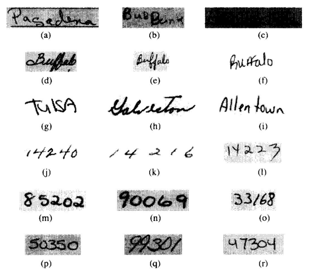
The durable systems lesson lies in the pipeline shared by these applications. Image capture and preprocessing constrained the model input, inference produced class scores, rejection thresholds traded automation coverage against error, and human review handled cases outside the accepted confidence range.
Engineering process and design decisions
Recognizing a clean, centered digit is straightforward. Recognizing handwriting amid variable backgrounds, scale, alignment, and image quality requires engineering decisions at every stage from data preparation to deployment.
The dataset histories must remain separate. Early ZIP-code research used postal digit images supplied for that task (LeCun et al. 1989). MNIST was later constructed from National Institute of Standards and Technology (NIST) handwritten-digit databases and standardized into size-normalized benchmark images (LeCun et al. 1998). It did not arise from collecting live envelopes under varying colors, textures, lighting, and orientations. Across both datasets, however, the engineering requirement was the same: preprocessing had to reduce irrelevant variation without erasing the stroke information needed for recognition.
Architecture design balances accuracy, processing time, and memory cost. For the chapter’s standardized \(28{\times}28\) digit input, the central question is how much model capacity the available latency and hardware budget can support.
Training must cover handwriting variation rather than optimize only for a curated test set. Preprocessing normalizes size and orientation, while augmentation can expose the model to additional plausible variation. Evaluation must then measure performance across relevant writing styles and operating conditions, following the systematic workflow described in ML Workflow.
Confidence thresholds determine the division of labor between automation and human review. A high threshold rejects more items for manual handling; a low threshold accepts more model errors. An expected-cost rule chooses threshold \(t\) to minimize \(\text{manual\_rate}(t)C_{\text{manual}} + \text{error\_rate}(t)C_{\text{error}}\) subject to throughput and latency constraints.
Shared pipeline architecture
Postal ZIP-code research and deployed bank-check readers used different operational systems, but both fit the pattern in figure 20. Image acquisition and conventional preprocessing prepare the input, neural inference produces digit scores, and postprocessing either accepts the result or routes an uncertain item for review. The figure presents this shared architecture as a composite systems pattern.
\begin{tikzpicture}[font=\small\sffamily, >=stealth]
\tikzset{
Box/.style={align=center, inner xsep=2pt,draw=GreenLine, line width=1pt,fill=none,
minimum width=24mm, minimum height=25mm,node distance=1.0},
LineA/.style={BrownLine!70,line width=4.0pt,{-{Triangle[width=1.5*6pt,length=2.0*5pt]}},shorten <=1pt,shorten >=1pt},
ALine/.style={black!50, line width=1.1pt,{{Triangle[width=0.9*6pt,length=1.2*6pt]}-}},
Larrow/.style={fill=violet!50, single arrow,  inner sep=2pt, single arrow head extend=3pt,
            single arrow head indent=0pt,minimum height=10mm, minimum width=3pt}
}
%inbox
\tikzset{%
 pics/inbox/.style = {
        code = {
        \pgfkeys{/channel/.cd, #1}
\begin{scope}[local bounding box=INBOX,scale=\scalefac, every node/.append style={transform shape}]
\node[line width=\Linewidth,draw=\drawcolor,fill=\filllcolor!50,
rectangle,rounded corners=3pt,minimum width=14mm,minimum height=10mm]at(0,0.3){};
\node[line width=\Linewidth,draw=\drawcolor,fill=\filllcolor,
rectangle,rounded corners=3pt,minimum width=15mm,minimum height=10mm]at(0,0.1){};
\node[line width=\Linewidth,draw=\drawcolor,fill=\filllcolor!50,
,rectangle,rounded corners=3pt,minimum width=17mm,minimum height=10mm]
at(0,-0.1){};
\draw[line width=\Linewidth,draw=\drawcolor,fill=\filllcirclecolor,,rounded corners=2pt](-0.92,0.05)--
(-0.92,-0.78)--(0.92,-0.78)--(0.92,0.05)--(0.40,0.05)--(0.32,-0.2)--(-0.29,-0.2)--(-0.40,0.05)--cycle;

\node[single arrow, line width=\Linewidth,draw=black,fill=cyan!90!black!30, rotate=270,
      minimum width = 15pt, single arrow head extend=6pt,
      minimum height=10mm]at(0,0.5) {}; % length of arrow
 \end{scope}
     }
  }
}
%brain
\tikzset{pics/brain/.style = {
        code = {
        \pgfkeys{/channel/.cd, #1}
\begin{scope}[local bounding box=BRAIN,scale=\scalefac, every node/.append style={transform shape}]
\fill[fill=\filllcolor!50](0.1,-0.5)to[out=0,in=180](0.33,-0.5)
to[out=0,in=270](0.45,-0.38)to(0.45,-0.18)
to[out=40,in=240](0.57,-0.13)to[out=110,in=310](0.52,-0.05)
to[out=130,in=290](0.44,0.15)to[out=90,in=340,distance=8](0.08,0.69)
to[out=160,in=80](-0.42,-0.15)to (-0.48,-0.7)to(0.07,-0.7)to(0.1,-0.5)
(-0.10,-0.42)to[out=310,in=180](0.1,-0.5);
\draw[draw=\drawcolor,line width=\Linewidth](0.1,-0.5)to[out=0,in=180](0.33,-0.5)
to[out=0,in=270](0.45,-0.38)to(0.45,-0.18)
to[out=40,in=240](0.57,-0.13)to[out=110,in=310](0.52,-0.05)
to[out=130,in=290](0.44,0.15)to[out=90,in=340,distance=8](0.08,0.69)
(-0.42,-0.15)to (-0.48,-0.7)
(0.07,-0.7)to(0.1,-0.5)
(-0.10,-0.42)to[out=310,in=180](0.1,-0.5);
\draw[fill=\filllcolor,line width=\Linewidth](-0.3,-0.10)to(0.08,0.60)
to[out=60,in=50,distance=3](-0.1,0.69)to[out=160,in=80](-0.26,0.59)to[out=170,in=90](-0.46,0.42)
to[out=170,in=110](-0.54,0.25)to[out=210,in=150](-0.54,0.04)
to[out=240,in=130](-0.52,-0.1)to[out=300,in=240]cycle;
\draw[fill=\filllcolor,line width=\Linewidth]
(-0.04,0.64)to[out=120,in=0](-0.1,0.69)(-0.19,0.52)to[out=120,in=330](-0.26,0.59)
(-0.4,0.33)to[out=150,in=280](-0.46,0.42)
%
(-0.44,-0.03)to[bend left=30](-0.34,-0.04)
(-0.33,0.08)to[bend left=40](-0.37,0.2) (-0.37,0.12)to[bend left=40](-0.45,0.14)
(-0.26,0.2)to[bend left=30](-0.24,0.13)
(-0.16,0.32)to[bend right=30](-0.27,0.3)to[bend right=30](-0.29,0.38)
(-0.13,0.49)to[bend left=30](-0.04,0.51);

\draw[rounded corners=0.8pt,\drawcircle,-{Circle[fill=\filllcirclecolor,length=2.5pt]}](-0.23,0.03)--(-0.15,-0.03)--(-0.19,-0.18)--(-0.04,-0.28);
\draw[rounded corners=0.8pt,\drawcircle,-{Circle[fill=\filllcirclecolor,length=2.5pt]}](-0.17,0.13)--(-0.04,0.05)--(-0.06,-0.06)--(0.14,-0.11);
\draw[rounded corners=0.8pt,\drawcircle,-{Circle[fill=\filllcirclecolor,length=2.5pt]}](-0.12,0.23)--(0.31,0.0);
\draw[rounded corners=0.8pt,\drawcircle,-{Circle[fill=\filllcirclecolor,length=2.5pt]}](-0.07,0.32)--(0.06,0.26)--(0.16,0.33)--(0.34,0.2);
\draw[rounded corners=0.8pt,\drawcircle,-{Circle[fill=\filllcirclecolor,length=2.5pt]}](-0.01,0.43)--(0.06,0.39)--(0.18,0.51)--(0.31,0.4);
\end{scope}
     }
  }
}
%llm
\tikzset{
pics/llm/.style = {
        code = {
        \pgfkeys{/channel/.cd, #1}
\begin{scope}[shift={($(0,0)+(0,0)$)},scale=\scalefac,every node/.append style={transform shape}]
\node[circle,minimum size=12mm,draw=\drawcolor, fill=\filllcolor!70,line width=0.5*\Linewidth](C\picname) at (0,0){};
\def\startangle{90}
\def\radius{1.15}
\def\radiusI{1.1}
\foreach \i [evaluate=\i as \j using \i+1] [count =\k] in {0,2,4,6,8} {
\pgfmathsetmacro{\angle}{\startangle - \i * (360/8)}
\draw[draw=black,-{Circle[black ,fill=\filllcirclecolor,length=5.5pt,line width=0.5*\Linewidth]},line width=1.5*\Linewidth](C\picname)--++(\startangle - \i*45:\radius) ;
\node[circle,draw=black,fill=\filllcirclecolor!80!red!50,inner sep=3pt,line width=0.5*\Linewidth](2C\k)at(\startangle - \j*45:\radiusI) {};
}
\draw[line width=1.5*\Linewidth](2C1)--++(-0.5,0)|-(2C2);
\draw[line width=1.5*\Linewidth](2C3)--++(0.5,0)|-(2C4);
\node[circle,,minimum size=12mm,draw=\drawcolor, fill=\filllcolor!70,line width=0.5*\Linewidth]at (0,0){};
\node[draw,rectangle,rounded corners=1pt,minimum width=7mm,minimum height=4mm,fill=orange!10](R1)at(0.1,0.1){};
\draw[BrownLine,shorten <=2pt,shorten >=2pt ]($(R1.north west)!0.35!(R1.south west)$)--($(R1.north east)!0.35!(R1.south east)$);
\draw[BrownLine,shorten <=2pt,shorten >=2pt ]($(R1.north west)!0.7!(R1.south west)$)--($(R1.north east)!0.7!(R1.south east)$);
\node[draw,rectangle,rounded corners=1pt,minimum width=6mm,minimum height=4mm,fill=orange!10](R2)at(-0.05,-0.15){};
\draw[BrownLine,shorten <=2pt,shorten >=2pt ]($(R2.north west)!0.35!(R2.south west)$)--($(R2.north east)!0.35!(R2.south east)$);
\draw[BrownLine,shorten <=2pt,shorten >=2pt ]($(R2.north west)!0.7!(R2.south west)$)--($(R2.north east)!0.7!(R2.south east)$);
\end{scope}
    }
  }
}
%funnel
\tikzset{%
 pics/funnel/.style = {
        code = {
        \pgfkeys{/channel/.cd, #1}
\begin{scope}[local bounding box=FUNNEL,scale=\scalefac, every node/.append style={transform shape}]
\draw[fill=\filllcolor,line width=\Linewidth,draw=\drawcolor](-0.12,-0.81)--(-0.19,-0.25)--(-0.7,0.41)--(0.7,0.41)--(0.19,-0.25)--(0.12,-0.81)--cycle;
\draw[fill=\filllcolor,line width=\Linewidth,draw=\drawcolor](-0.19,-0.25)--(0.08,-0.25);
\draw[fill=\filllcolor,line width=\Linewidth,draw=\drawcolor](0.16,-0.09)--(0.41,0.31);
%
\node[line width=\Linewidth,draw=\drawcolor,fill=\filllcolor,inner sep=1pt,
rectangle,rounded corners=2pt,minimum width=16mm,minimum height=5pt]at(0,0.5){};
%
\foreach \i in{-0.5,0,0.5}{
\node[single arrow, line width=0.8*\Linewidth,draw=black,fill=\filllcirclecolor, rotate=270,inner sep=1pt,
      minimum width =9pt, single arrow head extend=2pt,
      minimum height=5mm]at(\i,0.9) {}; % length of arrow
   }
\node[single arrow,line width=0.8*\Linewidth,draw=black,fill=\filllcirclecolor, rotate=270,inner sep=1pt,
      minimum width =11pt, single arrow head extend=2pt,
      minimum height=5mm]at(0,-1.1) {}; % length of arrow
 \end{scope}
     }
  }
}
\def\inset{2.0pt} %
\def\myshape{%
  (0,1.34) to[out=220,in=0] (-1.20,1.03) --
  (-1.20,-0.23) to[out=280,in=160] (0,-1.53) to[out=20,in=260] (1.20,-0.23) --
  (1.20,1.03)  to[out=180,in=320] cycle
}
\tikzset{
pics/stitC/.style = {
        code = {
        \pgfkeys{/channel/.cd, #1}
\begin{scope}[shift={($(0,0)+(0,0)$)},scale=\scalefac,every node/.append style={transform shape}]
\fill[fill=\filllcolor!60] \myshape;
%
\begin{scope}
  \clip \myshape;
  \draw[draw=\filllcolor!60, line width=3*\inset,fill=white] \myshape; % Color and thickness as desired
\end{scope}
\draw[red,line width=3pt](-0.7,-0.35)--++(320:0.5)--++(50:1.5);
\end{scope}
    }
  }
}
%gear-arrow
% #1 number of teeths
% #2 radius intern
% #3 radius extern
% #4 angle from start to end of the first arc
% #5 angle to decale the second arc from the first
% #6 inner radius to cut off
\tikzset{
  pics/gearAR/.style args={#1/#2/#3/#4/#5/#6/#7}{
   code={
           \pgfkeys{/channel/.cd, #7}
\begin{scope}[shift={($(0,0)+(0,0)$)},scale=\scalefac,every node/.append style={transform shape},
LinE/.style={\filllcirclecolor,line width=5.0pt,
{{Triangle[width=1.5*10pt,length=2.0*5pt]}-},shorten <=5pt,shorten >=1pt},
ELin/.style={\filllcirclecolor,line width=7.0pt,
{-{Triangle[width=1.15*10pt,length=2.0*5pt]}},shorten <=0pt,shorten >=0pt}]
    \pgfmathtruncatemacro{\N}{#1}%,
    \def\rin{#2}\def\rout{#3}\def\aA{#4}\def\aOff{#5}\def\rcut{#6}%
    \path[rounded corners=0.5pt,draw=\drawcolor,fill=\filllcolor]
      (0:\rin)
      \foreach \i [evaluate=\i as \n using (\i-1)*360/\N] in {1,...,\N}{%
        arc (\n:\n+\aA:\rin)
        -- (\n+\aA+\aOff:\rout)
        arc (\n+\aA+\aOff:\n+360/\N-\aOff:\rout)
        -- (\n+360/\N:\rin)
      } -- cycle;
      \draw[draw=none,fill=white](0,0) circle[radius=\rcut];
\draw[ELin](0,0)--++(0:2.5);
\end{scope}
  }}
}
%testing+pencil
\tikzset{
pics/testing/.style = {
        code = {
        \pgfkeys{/channel/.cd, #1}
\begin{scope}[local bounding box=TESTING1,shift={($(0,0)+(0,0)$)},scale=\scalefac,every node/.append style={transform shape}]
\newcommand{\tikzxmark}{%
\tikz[scale=0.18] {
    \draw[line width=0.7,line cap=round,RedLine] (0,0) to [bend left=6] (1,1);
    \draw[line width=0.7,line cap=round,RedLine] (0.2,0.95) to [bend right=3] (0.8,0.05);
}}
\newcommand{\tikzxcheck}{%
\tikz[scale=0.16] {
    \draw[line width=0.7,line cap=round,GreenLine] (0.5,0.75)--(0.85,-0.1) to [bend left=16] (1.5,1.55);

}}
 \node[draw, minimum width  =15mm, minimum height = 20mm, inner sep = 0pt,
        rounded corners,draw = \drawcolor, fill=\filllcolor!10, line width=\Linewidth](COM){};
\node[draw=GreenLine,inner sep=4pt,fill=white](CB1) at ($(COM.north west)!0.25!(COM.south west)+(0.3,0)$){};
\node[xshift=0pt]at(CB1){\tikzxcheck};
\node[draw=RedLine,inner sep=4pt,fill=white](CB2) at ($(COM.north west)!0.5!(COM.south west)+(0.3,0)$){};
\node[xshift=0pt]at(CB2){\tikzxmark};
\node[draw=RedLine,inner sep=4pt,fill=white](CB3) at ($(COM.north west)!0.75!(COM.south west)+(0.3,0)$){};
\node[xshift=0pt]at(CB3){\tikzxmark};
\draw[GreenLine,decoration={zigzag,segment length=4pt, amplitude=0.5pt},decorate]($(CB1)+(0.3,0.05)$)--++(0:0.8);
\draw[GreenLine,decoration={zigzag,segment length=4pt, amplitude=0.5pt},decorate]($(CB1)+(0.3,-0.12)$)--++(0:0.7);
\draw[RedLine,decoration={zigzag,segment length=4pt, amplitude=0.5pt},decorate]($(CB2)+(0.3,0.05)$)--++(0:0.8);
\draw[RedLine,decoration={zigzag,segment length=4pt, amplitude=0.5pt},decorate]($(CB2)+(0.3,-0.12)$)--++(0:0.6);
\draw[RedLine,decoration={zigzag,segment length=4pt, amplitude=0.5pt},decorate]($(CB3)+(0.3,0.05)$)--++(0:0.8);
\draw[RedLine,decoration={zigzag,segment length=4pt, amplitude=0.5pt},decorate]($(CB3)+(0.3,-0.12)$)--++(0:0.6);
\end{scope}
    }
  }
}
%pencil
\tikzset{
pics/pencil/.style = {
        code = {
        \pgfkeys{/channel/.cd, #1}
\begin{scope}[local bounding box=TESTING1,shift={($(0,0)+(0,0)$)},scale=\scalefac,every node/.append style={transform shape},rotate=340]
            \fill[fill=\filllcolor!70] (0,4) -- (0.4,4) -- (0.4,0) --(0.3,-0.15) -- (0.2,0) -- (0.1,-0.14) -- (0,0) -- cycle;
            \draw[color=white,thick] (0.2,4) -- (0.2,0);
            \fill[black] (0,3.5) -- (0.2,3.47) -- (0.4,3.5) -- (0.4,4) arc(30:150:0.23cm);
            \fill[fill=\filllcolor!40] (0,0) -- (0.2,-0.8)node[coordinate,pos=0.75](a){} -- (0.4,0)node[coordinate,pos=0.25](b){} -- (0.3,-0.15) -- (0.2,0) -- (0.1,-0.14) -- cycle;
            \fill[fill=\filllcolor] (a) -- (0.2,-0.8) -- (b) -- cycle;

\end{scope}
    }
  }
}
\pgfkeys{
  /channel/.cd,
   Depth/.store in=\Depth,
  Height/.store in=\Height,
  Width/.store in=\Width,
  filllcirclecolor/.store in=\filllcirclecolor,
  filllcolor/.store in=\filllcolor,
  drawcolor/.store in=\drawcolor,
  drawcircle/.store in=\drawcircle,
  scalefac/.store in=\scalefac,
  Linewidth/.store in=\Linewidth,
  picname/.store in=\picname,
  filllcolor=BrownLine,
  filllcirclecolor=violet!20,
  drawcolor=black,
  drawcircle=violet,
  scalefac=1,
  Linewidth=0.5pt,
  Depth=1.3,
  Height=0.8,
  Width=1.1,
  picname=C
}
%Raw Data
\node[Box](B1){};
\fill[cyan!07](B1.north west) rectangle ($(B1.north east)!0.6!(B1.south east)$)coordinate(B1DE);
\fill[cyan!20](B1.south east) rectangle ($(B1.north west)!0.6!(B1.south west)$)coordinate(B1LE);
\node[Box,draw=BlueD](){};
\tikzset{Text2/.style={font=\sffamily\bfseries\small,align=center}}
\node[Text2]at($(B1.south west)!0.5!(B1DE)$){Raw Data};
\coordinate(Q1)at($(B1.north west)!0.5!(B1DE)$);
\pic[shift={(0,0)}] at  (Q1){inbox={scalefac=0.7,picname=1,Linewidth=1.0pt,
 filllcolor=BrownL,drawcolor=black,filllcirclecolor=orange!70!yellow!80}};
%Preprocessing
\node[Box, right=0.75 of B1](B2){};
\fill[cyan!07](B2.north west) rectangle ($(B2.north east)!0.6!(B2.south east)$)coordinate(B2DE);
\fill[cyan!20](B2.south east) rectangle ($(B2.north west)!0.6!(B2.south west)$)coordinate(B2LE);
\node[Box, right=0.75 of B1,draw=BlueD](B2){};
\node[Text2]at($(B2.south west)!0.5!(B2DE)$){Pre-\\processing};
\coordinate(Q2)at($(B2.north west)!0.5!(B2DE)$);
\pic[shift={(0,0)}] at  (Q2){funnel={scalefac=0.53,picname=1,Linewidth=0.5pt,
 filllcolor=green!70!orange!70,drawcolor=black,filllcirclecolor=red!70!blue!80}};
%Neural Network
\node[Box, right=of B2](B3){};
\fill[green!07](B3.north west) rectangle ($(B3.north east)!0.6!(B3.south east)$)coordinate(B3DE);
\fill[green!20](B3.south east) rectangle ($(B3.north west)!0.6!(B3.south west)$)coordinate(B3LE);
\node[Box, right=of B2,draw=GreenD](B3){};
\node[Text2]at($(B3.south west)!0.5!(B3DE)$){Neural\\ Network};
\coordinate(Q3)at($(B3.north west)!0.5!(B3DE)$);
%\pic[shift={(0,0)}] at  (Q3){brain={scalefac=0.9,picname=1,filllcolor=orange!30!, Linewidth=0.95pt}};
\pic[shift={(0,0)}] at  (Q3){llm={scalefac=0.6,drawcolor=BlueLine,filllcolor=BlueLine!50!, Linewidth=1pt,filllcirclecolor=red}};
%Raw output
\node[Box, right=of B3](B4){};
\fill[violet!07](B4.north west) rectangle ($(B4.north east)!0.6!(B4.south east)$)coordinate(B4DE);
\fill[violet!20](B4.south east) rectangle ($(B4.north west)!0.6!(B4.south west)$)coordinate(B4LE);
\node[Box, right=of B3,draw=VioletLine](B4){};
\node[Text2]at($(B4.south west)!0.5!(B4DE)$){Raw\\ Output};
\coordinate(Q4)at($(B4.north west)!0.5!(B4DE)$);
 \pic[shift={(0,0)}] at (Q4) {gearAR={14/1.4/1.8/8/4/0.7/scalefac=0.35,drawcolor=BlueLine,filllcolor=BlueLine,filllcirclecolor=red}};
%Postprocessing
\node[Box, right=0.75of B4](B5){};
\fill[violet!05](B5.north west) rectangle ($(B5.north east)!0.6!(B5.south east)$)coordinate(B5DE);
\fill[violet!15](B5.south east) rectangle ($(B5.north west)!0.6!(B5.south west)$)coordinate(B5LE);
\node[Box, right=0.75of B4,draw=VioletLine](B5){};
\node[Text2]at($(B5.south west)!0.5!(B5DE)$){Post-\\processing};
\coordinate(Q5)at($(B5.north west)!0.5!(B5DE)$);
\pic[shift={(0,0)}] at  (Q5){testing={scalefac=0.65,picname=1,drawcolor=myblue,filllcolor=myblue, Linewidth=1.0pt}};
\pic[shift={(0,-0.5)},rotate=-15] at  (Q5){pencil={scalefac=0.30,picname=1,filllcolor=mygreen, Linewidth=1.0pt}};
%%%%%%
%Final output
\node[Box, right= 0.75of B5](B6){};
\fill[violet!05](B6.north west) rectangle ($(B6.north east)!0.6!(B6.south east)$)coordinate(B6DE);
\fill[violet!15](B6.south east) rectangle ($(B6.north west)!0.6!(B6.south west)$)coordinate(B6LE);
\node[Box, right=0.75of B5,draw=VioletLine]{};
\node[Text2]at($(B6.south west)!0.5!(B6DE)$){Final Output};
\coordinate(Q6)at($(B6.north west)!0.5!(B6DE)$);
\pic[shift={(0,0.05)}] at  (Q6){stitC={scalefac=0.45,drawcolor=orange,filllcolor=green!55!black}};
%arrows
\foreach \i in{1,2,3,4,5}{
\pgfmathtruncatemacro{\X}{\i + 1} %
\draw[LineA](B\i)--(B\X);
}
\node[draw=myblue,line width=0.75pt,fit=(B1)(B2),inner ysep=3mm,inner xsep=4mm,xshift=1mm](F1){};
\node[draw=none,fit=(B3),inner ysep=3mm,inner xsep=4mm](F2){};
\node[draw=mypurple,line width=0.75pt,fit=(B4)(B6),inner ysep=3mm,inner xsep=4mm,xshift=-1mm](F3){};
\node[below =0pt of F1,text=myblue]{Preprocessing};
\node[below =0pt of F2,text=GreenD]{Deep Learning};
\node[below =0pt of F3,text=mypurple]{Postprocessing};
\end{tikzpicture}The pipeline begins with image acquisition. In postal research, the input was an image of a handwritten ZIP-code region; deployed check readers similarly began with scanned document images. Acquisition quality determines how much variation the later preprocessing and recognition stages must absorb.
Preprocessing locates the relevant field, separates or otherwise identifies its characters, and normalizes the resulting images. Thresholding, connected-component analysis, and size normalization are representative conventional techniques. The chapter uses standardized \(28{\times}28\) images for its MNIST calculations; that dimension is a teaching convention here, not a claim about every postal or check-reading deployment.
The neural network then processes each normalized digit image. The 1989 ZIP-code research system used an early LeNet variant (LeCun et al. 1989) with approximately 10,000 parameters, remarkably compact compared with the 109.4K in this chapter’s MNIST network. Both produce digit scores through layered neural computation, although their architectures and operating contexts differ.
Postprocessing converts digit scores into application decisions. For a ZIP-code task, one uncertain digit can send the complete code for further processing or human review. Deployed document readers use the same general principle: accept sufficiently confident predictions and reject uncertain cases instead of forcing an answer.
Deployed document readers must satisfy end-to-end timing constraints spanning acquisition, preprocessing, inference, postprocessing, and downstream action. The exact machinery differs between mail and financial-document applications, but throughput depends on the complete pipeline rather than neural-network latency alone.
Performance outcomes and operational impact
The 1989 ZIP-code study reported its model, recognition, throughput, and training measurements as one experimental system. Table 14 keeps those measurements together, revealing how rejection policy and preprocessing affect the meaning of raw classifier speed (LeCun et al. 1989).
LeCun, Yann, Bernhard Boser, John S. Denker, Donald Henderson, Richard E. Howard, Wayne Hubbard, and Lawrence D. Jackel. 1989. “Backpropagation Applied to Handwritten Zip Code Recognition.” Neural Computation 1 (4): 541–51. https://doi.org/10.1162/neco.1989.1.4.541.
| Metric | Reported Result |
|---|---|
| Error and rejection | 1% classification error after rejecting 12.1% of test digits |
| Throughput | 10–12 classifications/sec including acquisition; over 30/sec after normalization |
| Model parameters | ~10,000 |
| Training | 23 passes; about 3 days on a Sun-4/260 workstation |
The measurements tell a systems story rather than an accuracy story. The ZIP-code experiment showed that learned recognition could handle realistic handwritten digits with an explicit rejection policy. By the late 1990s, related LeNet-based bank-check readers were processing documents at commercial scale (LeCun et al. 1998). These were separate milestones, joined by the decision to preserve a path for uncertain inputs.
LeCun, Yann, Léon Bottou, Yoshua Bengio, and Patrick Haffner. 1998. “Gradient-Based Learning Applied to Document Recognition.” Proceedings of the IEEE 86 (11): 2278–324. https://doi.org/10.1109/5.726791.
The rejection path, not the raw error rate, is what made the deployment work. Uncertain cases went to human operators rather than forcing every example through the model, so the system bought reliability by choosing where to stop trusting the network.
Performance depends on how closely operating inputs match the variation represented during training. Image quality, writing style, and preprocessing behavior can all shift recognition accuracy, so the physical and statistical pipeline must be evaluated together.
The economic mechanism comes from shifting the operating point, not from eliminating people entirely. Automation handles high-confidence digits, while human operators resolve uncertain cases and preserve a fallback for inputs outside the model’s reliable regime.
This history also identifies durable production requirements. Teams must monitor input quality and rejection rates, update training data when operating distributions change, and maintain both the recognition model and its surrounding acquisition and preprocessing machinery. These are lifecycle implications of the combined systems pattern, not documented features of one USPS deployment.
Key engineering lessons and design principles
Across postal ZIP-code research and deployed check readers, the central lesson is that neural computation succeeds only when the surrounding pipeline shares the same operating constraint. Preprocessing, inference, postprocessing, rejection, and downstream action must support the required throughput and error budget together.
This combined history shows why theoretical foundations and systems integration both matter. Converting handwritten marks into reliable operational decisions required coordinated choices in network architecture, training, preprocessing, confidence policy, and downstream handling.
Taken together, the research demonstrations and later document-reader deployments illustrate practices that remain standard: representative training data, confidence metrics, pre- and postprocessing, rejection paths, and end-to-end optimization. These operational considerations are formalized in ML Operations.
Modern edge systems operate under different power, latency, and deployment constraints, but the same engineering principles apply: preprocessing for real-world variation, confidence-based routing to human review, and end-to-end pipeline optimization. The combined document-recognition history therefore supplies a reusable systems pattern without treating postal research, check-reader deployment, and MNIST as one application.
Systems Perspective 1.6: Reading historical system comparisons
The early LeNet-class reader and this chapter’s MNIST multilayer perceptron show continuity in computation, not a controlled performance benchmark. Their datasets, architectures, software stacks, machines, and operating targets differ. The defensible comparison is structural: both transform normalized pixels into digit scores, both depend on learned parameters and a preprocessing pipeline, and both need an explicit policy for uncertain outputs.
Parameter count supplies one concrete contrast. The 1989 ZIP-code network had approximately 10,000 parameters, while the chapter’s fully connected network has 109,386. That difference describes model state; it does not by itself establish latency, energy, throughput, or cost. Those outcomes require a fixed workload and measurements that identify the hardware, numerical precision, runtime, batch size, and end-to-end decision path. Separating these variables prevents a faster deployment from being attributed entirely to silicon when the data, model, software, or operating policy also changed.
This combined history is one instance of a broader alignment pattern: successful ML systems coordinate the task, its data, the algorithm, and the machine. The next section formalizes that pattern.
Self-Check: Question
Which set of operational performance metrics accurately matches the benchmark results reported for the 1989 USPS handwritten digit recognition prototype developed by LeCun et al.?
- \(0\%\) error rate at \(0\%\) rejection rate, processing over \(1{,}000\) mailpieces per second.
- \(10\%\) error rate at \(50\%\) rejection rate, operating exclusively as an offline batch indexing system.
- \(5\%\) error rate at \(2\%\) rejection rate, requiring human video coding for every mailpiece.
- \(1\%\) error rate achieved at a \(12.1\%\) rejection rate, processing \(10\text{–}12\) classifications per second end-to-end and over \(30\) digits per second on pre-normalized inputs.
The chapter presents an illustrative ‘Then vs. Now’ comparison showing that running the 1989 LeNet architecture on modern edge silicon achieves \(\approx 1{,}000\times\) lower latency and \(\approx 20{,}000\times\) lower energy per inference. What is the fundamental systems engineering takeaway from this analysis?
- The algorithmic model was completely redesigned, accounting for all observed throughput gains.
- Semiconductor and accelerator advances multiplied the viable deployment envelope of the same neural computation, while core pipeline principles (preprocess, infer, threshold, route) remained durable.
- Modern edge accelerators eliminate the need for confidence thresholds and manual human review.
- Optical scanning and digit segmentation preprocessing are no longer necessary on modern hardware.
In the USPS postal sorting pipeline, explain why setting the rejection threshold to zero (forcing an automated prediction on \(100\%\) of mailpieces) is economically and operationally undesirable.
Describe how the 1989 USPS digit recognition system decomposed the document recognition challenge into a multi-stage pipeline, and explain why the neural classifier alone was not sufficient.
In the USPS document recognition pipeline, the preprocessing operation that isolates individual handwritten character bounding boxes from a continuous multi-digit ZIP code block is termed digit ____.
Order the physical and computational stages of the end-to-end USPS mail sorting pipeline: (1) Route accepted mail to physical sorting bins or rejected mail to human review, (2) Evaluate confidence thresholds on model output probabilities to accept or reject predictions, (3) Optically scan the mailpiece envelope to capture raw image data, (4) Execute neural network forward inference on normalized digit tensors, (5) Locate the ZIP code region, segment individual digits, and scale-normalize them.
D·A·M Taxonomy
Across the document-recognition histories, different resources served different purposes. USPS-supplied ZIP images grounded early recognition research, LeNet supplied an algorithmic mechanism, later bank-check readers supplied a documented deployment setting, and MNIST supplied a standardized benchmark derived from NIST data. They do not form one system, but together they show the three questions in the D·A·M taxonomy: does the data represent the task, can the algorithm learn the required behavior, and can the machine execute it within the operating budget? The D·A·M Taxonomy develops the intersections among these axes.
The Data axis asks whether the examples and labels describe the behavior the deployed system must recognize. The USPS ZIP-code images, MNIST digits, and bank-check inputs are related but not interchangeable: each embodies a different acquisition process, input distribution, and operating goal. Preprocessing can normalize some variation, but it cannot create missing handwriting styles or repair a label policy that does not match the downstream decision. Data also has a physical footprint. Batch size, image resolution, numerical representation, and storage layout determine how many bytes must enter the training or inference pipeline.
The Algorithm axis asks what transformation can learn the desired behavior from that evidence. In the running network, the 784-to-128 first layer determines both the model’s initial representational capacity and its dominant parameter count. Activation functions determine which nonlinear boundaries can be expressed and how gradients propagate; the loss and optimizer determine which errors drive parameter updates. These choices shape the work the system must perform, but an elegant learning rule is useful only if its assumptions match the data and its operations fit the deployment budget.
The Machine axis asks whether those operations can execute with the required latency, throughput, memory capacity, and energy. Forward propagation moves parameters and activations through matrix operations; backpropagation adds saved values, gradients, optimizer state, and a reverse dependency traversal. Batch size can increase reuse while expanding activation storage. Lower precision can reduce bytes and expose faster kernels, but only after task-level evaluation shows that the resulting numerical error is acceptable. The machine therefore constrains not only how quickly a fixed network runs, but also which network, batch, and precision are feasible.
The pairwise intersections explain why the axes cannot be optimized independently. Data and Algorithm determine what the system can learn from; Data and Machine determine how information is represented and moved; Algorithm and Machine determine how the computation executes efficiently. At the center, all three questions must be answered together. A larger dataset may improve coverage while increasing input traffic, a wider network may improve capacity while exceeding memory, and a lower-precision kernel may improve throughput while changing accuracy.
The chapter’s computations make this diagnostic procedure concrete. Begin with an observed symptom such as low accuracy, missed latency, or exhausted memory. Form competing hypotheses on all three axes, then measure the quantity that distinguishes them: coverage and label quality for Data, error slices and learning behavior for Algorithm, or utilization, bandwidth, and capacity for Machine. An intervention on one axis can move the bottleneck to another, so the final test is always end-to-end behavior under the intended workload. The D·A·M Taxonomy turns this first-pass diagnosis into a detailed map of the intersection techniques used throughout the book.
These foundations equip engineers to reason about neural networks from first principles. Yet conceptual understanding alone is insufficient: practitioners must also recognize the recurring misconceptions that derail real-world projects.
Self-Check: Question
Under the D·A·M (Data, Algorithm, Machine) taxonomy presented in the chapter, which statement correctly describes the primary responsibility of each axis and their systems interplay?
- Data determines GPU clock speed, Algorithm dictates physical memory capacity, and Machine formats training labels.
- Algorithm determines whether data is collected, Machine ensures 100% training accuracy, and Data operates independently of both.
- Data, Algorithm, and Machine can be optimized independently without cross-axis trade-offs.
- Algorithm defines computational transformations and capacity, Data determines whether the model can learn the task from representative evidence, and Machine determines whether those operations execute within latency, throughput, memory, and energy budgets.
A computer vision model deployed in production exhibits high accuracy during offline benchmark evaluations but suffers severe error rates on live camera feeds, while hardware GPU utilization is only \(15\%\). Use the D·A·M taxonomy to outline a structured diagnostic sequence to isolate the root causes.
According to the D·A·M taxonomy, if a deployed computer vision model suffers elevated error rates in production due to a distribution shift in ambient lighting and camera angles, why will scaling the Machine axis (allocating a larger cluster of faster GPUs) fail to resolve the operational failure?
- Hardware accelerators automatically reduce optimizer learning rates when cluster size increases.
- Faster GPU accelerators cannot process image tensors captured at non-standard aspect ratios.
- Machine scaling accelerates computational throughput but cannot supply the missing visual patterns or domain coverage required on the Data axis to learn the shifted distribution.
- The D·A·M framework requires all production deployments to execute on single-thread CPU cores.
Fallacies and Pitfalls
Statistical learning adds failure modes that line-by-line code inspection alone cannot reveal. The following fallacies and pitfalls can lead teams to misallocate effort or deploy inappropriate solutions.
Fallacy: Neural networks are entirely opaque and cannot be debugged.
Neural networks do not offer the line-by-line causal trace of traditional code, but they are not beyond diagnosis. Activation visualization can reveal learned patterns, gradient analysis measures local input sensitivity, and ablation studies estimate component contributions. These tools provide partial evidence rather than a complete explanation: saliency can be unstable, correlated features complicate attribution, and an ablation may change the behavior it is meant to probe. For the MNIST classifier in section 1.2.2, first-layer weights can still provide a useful check on what patterns the model has learned. Debugging a statistical system therefore combines model-level probes with data slices, controlled interventions, and end-to-end evaluation.
Pitfall: Discarding domain expertise because a deep model is available.
Teams assume automatic feature learning removes the need for domain knowledge. Successful systems require domain expertise at every stage: architecture selection, training objective design, dataset curation, and output interpretation. The document-recognition history in section 1.5 shows why confidence thresholds must reflect operating economics and route uncertain cases to human operators. Without domain knowledge, teams can deploy networks that look strong on a test set but fail in production because their thresholds, fallback paths, or error costs are wrong.
Fallacy: Deeper networks are always more accurate than wider ones.
Engineers assume that stacking more layers is the primary path to higher accuracy, since depth enables hierarchical feature extraction. In practice, depth alone encounters diminishing returns. ResNet showed that very deep residual networks can train effectively, but its ImageNet results also make clear that more layers must be weighed against added training and inference cost (He et al. 2016). EfficientNet later demonstrated that compound scaling of width, depth, and input resolution can outperform depth-only scaling at a given resource budget (Tan and Le 2019). The lesson is not that depth is bad; it is that teams should profile capacity utilization and scale the architecture dimension that gives the best accuracy per FLOP.
He, Kaiming, Xiangyu Zhang, Shaoqing Ren, and Jian Sun. 2016. “Deep Residual Learning for Image Recognition.” 2016 IEEE Conference on Computer Vision and Pattern Recognition (CVPR), 770–78. https://doi.org/10.1109/cvpr.2016.90.
Tan, Mingxing, and Quoc V Le. 2019. “EfficientNet: Rethinking Model Scaling for Convolutional Neural Networks.” International Conference on Machine Learning (ICML), 6105–14.
Pitfall: Using neural networks for problems solvable with simpler methods.
Teams assume deep learning always performs better. On small datasets or approximately linear relationships, a simpler model such as logistic regression may match or outperform a neural network while requiring less training, memory, and maintenance. The magnitude of that advantage is workload dependent, so teams should benchmark a simple baseline and justify added complexity through measured task-specific gains. Neural networks excel at hierarchical pattern discovery (section 1.1.3) but impose additional overhead. Use them when their representation capacity produces enough benefit to justify the measured systems cost.

Small neural workloads stay memory-bound even on large GPUs.
Fallacy: Training data distribution issues can be fixed after model design.
Teams treat training as mechanically feeding data through architectures. Networks on imbalanced datasets can exhibit poor minority-class performance: a fraud detector with 99:1 imbalance achieves 99 percent accuracy by always predicting “not fraud” while catching zero fraud cases. An unweighted average empirical-risk objective can underweight rare but critical classes unless sampling, weighting, loss design, and evaluation address the imbalance. Teams that skip exploratory data analysis may deploy models with strong aggregate metrics but unacceptable minority-class performance.
Pitfall: Deploying research models to production without addressing system constraints.
Production adds constraints absent from research: latency budgets (50–100 ms end-to-end), memory limits (2–4 GB for edge devices), and concurrent loads (100–1,000 requests per second (RPS)). The complete pipeline includes preprocessing, inference, and postprocessing (section 1.4). A model achieving 20 ms inference fails its 50 ms budget when preprocessing adds 25 ms and postprocessing adds 10 ms (55 ms total). Separating model development from system design therefore wastes effort on accuracy while ignoring deployment feasibility.
Fallacy: More compute automatically means faster training.
Teams purchase expensive GPUs expecting proportional speedups, but memory traffic or launch overhead may bind performance instead. Arithmetic intensity identifies the binding resource. Under a simple traffic model that reads the parameters once and moves each batch activation once, the MNIST forward pass in table 11 reaches approximately 12.4 FLOP/byte at batch 32 and still less at batch 1. This lies far below the ridge points of many high-throughput accelerators. The Roofline Model in The Roofline model explains why additional peak FLOP/s cannot help until the workload supplies enough reusable work per byte. Caches, fusion, vectorization, and launch cost make measured speedup the final test.
Pitfall: Extrapolating accuracy improvements without considering diminishing returns.
Teams may extrapolate a 5-point gain from scaling 10K parameters to 100K into another 5-point gain at 1M. Empirical improvement instead diminishes with scale according to the task, metric, data quality, model family, and scaling regime. Within table 5, the ImageNet rows show error falling from AlexNet’s 15.3 percent to ResNet-152’s 3.6 percent while training FLOPs rise from \(5 \times 10^{17}\) to roughly \(10^{19}\). Teams must therefore measure marginal return in their own regime rather than extrapolate linearly.
These fallacies and pitfalls share a common root: treating statistical behavior as if code behavior alone determined it. Recognizing them early directs attention toward the appropriate measurements and diagnostics.
Self-Check: Question
An engineering team migrates a small multilayer perceptron inference workload with low arithmetic intensity from a CPU to a high-end GPU featuring \(10\times\) higher peak TFLOP/s, but observes less than a \(1.2\times\) end-to-end speedup. Which systems explanation correctly diagnoses this outcome?
- The workload has low arithmetic intensity (FLOPs per byte) and is memory bandwidth-bound, meaning execution time is dominated by streaming parameters and activations from memory rather than floating-point computation in ALUs.
- The GPU driver automatically converts floating-point matrix multiplications into sequential scalar instructions.
- Neural networks are prohibited from executing in parallel on GPUs if their parameter count is under one million.
- The loss function becomes non-differentiable when running on accelerator hardware.
On a fraud detection dataset where \(99.5\%\) of transactions are legitimate and \(0.5\%\) are fraudulent, a newly trained classifier achieves \(99.4\%\) aggregate accuracy on held-out test data. Why is this aggregate metric deceptive from an ML systems engineering standpoint?
- Cross-entropy loss is undefined when class proportions differ by more than \(10\times\).
- An accuracy of \(99.4\%\) exceeds the theoretical mathematical limit of floating-point representation.
- A naive baseline that blindly predicts ‘legitimate’ for every transaction achieves \(99.5\%\) accuracy; an aggregate \(99.4\%\) accuracy can conceal a near-\(100\%\) failure rate on detecting actual fraud cases.
- High accuracy on an imbalanced dataset causes immediate GPU out-of-memory errors during inference.
A development team attempts to improve model accuracy by repeatedly stacking additional layers to a neural network (scaling depth alone) without modifying layer widths or input resolution. Why does this depth-only scaling strategy typically suffer from diminishing returns and training instability?
- Adding layers automatically reduces total parameter count by compressing intermediate representations.
- Increasing depth alone elongates the backpropagation chain-rule path, amplifying vanishing and exploding gradient risks while increasing sequential execution latency, without providing the balanced capacity gains of compound scaling across width, depth, and resolution.
- Modern GPU hardware architectures cannot allocate computational graphs with more than 10 layers.
- Deeper networks are legally restricted from using nonlinear activation functions.
A colleague argues that ‘because neural networks contain millions of weights functioning as an uninterpretable black box, they cannot be systematically debugged when prediction errors occur.’ Refute this claim by describing three concrete systems diagnostic techniques used to debug neural models.
During a model training run, an engineer observes that training loss continuously decreases across 50 epochs, but validation loss reaches a minimum at epoch 20 and increases steadily thereafter. Diagnose the model’s operational regime and describe two systems interventions to resolve it.
True or False: For a tabular dataset with 500 records and linear relationships between features and targets, deploying a deep neural network is generally superior to a linear regression model because deep networks inherently generalize better across all problem scales.
Summary
Neural computation translates mathematical formulations into physical machine execution. Linear algebra and calculus determine operation cost under the iron law of ML systems (\(T = \frac{D_{\text{vol}}}{\text{BW}} + \frac{O}{R_{\text{peak}} \cdot \eta_{\text{hw}}} + L_{\text{lat}}\)). Forward propagation establishes the computational work \(O\), often dominated by matrix multiplications, while backpropagation retains selected intermediate values and adds gradients and optimizer state. The resulting memory volume \(D_{\text{vol}}\) depends on architecture, batch size, precision, optimizer, and recomputation strategy. These mechanics make memory footprints, arithmetic intensities, and latency limits estimable before deployment.
Neural networks replace some hand-written decision rules and features with parameters learned from data. Weighted sums, nonlinear activations, and gradient-based learning provide recurring operations from which many modern architectures are composed.
Neural network architecture demonstrates hierarchical processing, where layers can transform raw inputs into representations useful for prediction. Training adjusts connection weights through iterative optimization, while inference applies the learned parameters to new data. These phases create different requirements for computation, memory, throughput, and latency. In this chapter’s simplified FP32 ledger, a batch-32 training step requires ~3.4× the memory of batch-32 inference because it adds gradients, optimizer state, and saved activations; the ratio changes with optimizer, precision, checkpointing, and architecture. The document-recognition case study showed how these mathematical principles enter a production pipeline in which preprocessing, neural inference, rejection, and postprocessing must satisfy one latency and reliability budget.
Key Takeaways: The math behind the model
- Each paradigm shift changes the systems cost of representation: In this \(28{\times}28\) digit example, the operation count rises from ~100 comparisons (rule-based) through ~8,000 operations (classical ML) to 109,184 MACs (deep learning)—a 1,091.8× scenario increase that reshapes hardware requirements.
- Neural networks learn representations from data: These networks replace some hand-coded features with hierarchical representations learned from examples. That flexibility shifts the burden toward representative data, training compute, and validation.
- Training and inference often emphasize different objectives: Training commonly favors efficient throughput across repeated updates, while online inference commonly favors per-request latency; offline inference may favor throughput instead. Batch size links utilization, memory, throughput, latency, and statistical behavior across these regimes.
- Activations are math and hardware: ReLU is generally cheaper to implement than sigmoid or tanh, and its unit gradient for positive inputs avoids activation saturation on that branch. Its practical advantage combines implementation cost with optimization behavior.
- Forward propagation often centers on matrix work: Dense matrix kernels exceed 90 percent of FLOPs in this chapter’s dense-network example and dominate many important neural workloads, which is why specialized matrix hardware can substantially outperform general-purpose execution for those operations.
- Backpropagation needs the path: Solving credit assignment requires retaining or recomputing the values used by the backward pass, so memory cost often determines whether a model can be trained on a given device and motivates techniques that reduce, recompute, or partition training state.
- The complete ML pipeline determines end-to-end performance: Preprocessing, neural computation, and postprocessing all contribute to latency and reliability. The document-recognition examples demonstrated that production success depends on the entire pipeline operating within real-world constraints, not on model accuracy on a test set alone.
The running MNIST example made this escalation tangible: the same 28 by 28 digit that required about 100 comparisons demanded 109,184 MACs in even a modest three-layer network—a 1,091.8× increase that generalizes across the systems dimensions captured in table 3. These fundamentals primarily develop the algorithm axis of the D·A·M taxonomy while revealing how algorithmic choices propagate into machine constraints.
The mathematical and systems implications emerge through fully connected architectures. The multilayer perceptrons explored here expose a direct resource law: dense connectivity makes both parameter storage and multiply-accumulate count scale with adjacent layer dimensions. This flexibility comes with computational costs. A 28 by 28 MNIST image contains 784 input values, and the first fully connected layer learns 100,352 weights by connecting every input to 128 neurons. That dense connectivity contains no explicit prior for spatial locality: the model must learn from data which nearby and distant pixel relationships matter, while paying to store and evaluate every connection.
These foundations establish the mathematical and systems vocabulary for reasoning about neural network behavior. The forward-backward propagation cycle, activation function choices, and memory-computation trade-offs recur throughout every subsequent chapter, whether analyzing why certain architectures train faster, why lower-precision approximations preserve accuracy in some layers but not others, or why multi-machine training requires careful coordination. Understanding these fundamentals enables engineers to move beyond treating neural networks as black boxes toward principled system design.
Reading the code reveals what a network is asked to do; reading the math reveals what it will cost to do it. That is why this chapter dwells on the arithmetic. A neural network is a point where the algorithm meets the machine: weights must be stored and moved, dense layers map to matrix operations, and saved activations make claims on memory that can determine whether the model fits. The math is where an algorithm signs its contract with the hardware, committing in advance to operations the machine must execute. Reading that contract lets an engineer estimate likely bottlenecks before profiling confirms where the network is fast and where it stalls.
What’s Next: From universal to specialized
Building on the system taxonomy established in ML Systems and the end-to-end pipeline requirements in ML Workflow, this chapter showed how generic fully connected networks turn every input-to-neuron connection into memory volume \(D_{\text{vol}}\) and compute work \(O\). Real-world data has exploitable structure: images exhibit spatial locality, text contains ordered and contextual dependencies, and time-series data contains temporal patterns. Network Architectures develops specialized architectures such as convolutions and self-attention that encode different structural assumptions. Those choices can reduce some forms of redundant work or improve reuse, but they also introduce new trade-offs in activation storage, memory access, arithmetic intensity, and accelerator parallelization.
Self-Check: Question
What is the chapter’s fundamental conclusion regarding why machine learning systems engineers must understand the mathematical primitives inside neural networks?
- Because deployment failures are primarily syntax errors in framework Python code.
- Because systems engineers are expected to manually derive and hand-code backpropagation routines for every production model.
- Because mathematical operators (matrix multiplications, activations, loss functions, and gradients) establish the Silicon Contract—directly defining the operation count \(O\), memory volume \(D_{\text{vol}}\), numerical stability, and hardware utilization that govern physical execution.
- Because neural network architectures change too rapidly for hardware accelerators to support standardized linear algebra primitives.
Compare the systems priorities, memory demands, and optimization objectives of neural network training versus inference for the same model architecture.
In the iron law of ML systems (\(T = \frac{D_{\text{vol}}}{\text{BW}} + \frac{O}{R_{\text{peak}} \cdot \eta_{\text{hw}}} + L_{\text{lat}}\)), the computational bargain where model architecture operators dictate the operation count \(O\) and memory volume \(D_{\text{vol}}\), while hardware and software determine realized bandwidth, latency, and throughput, is defined as the ____ contract.
Self-Check Answers
Self-Check: Answer
A team replaces a hand-coded digit recognition system (\(\approx 100\) conditional comparisons, \(784\text{ bytes}\) of working state) with a \(784 \to 128 \to 64 \to 10\) MLP (\(\approx 109{,}184\text{ MACs}\), \(\approx 438\text{ KB}\) of weights) on the same MNIST input. Which systems consequence should they expect when deploying this new model on a commodity CPU?
- The workload becomes dominated by branch mispredictions because artificial neurons execute frequent if-then branching decisions.
- The workload transitions from branch-heavy scalar code to dense matrix arithmetic whose weight footprint exceeds L1 cache capacity, generating cache-level memory traffic absent in the rule-based system.
- Execution memory traffic drops to zero because the \(438\text{ KB}\) weight footprint fits entirely within standard CPU register files.
- The model executes without using arithmetic logic units (ALUs) because learned representations bypass hardware compute pipelines.
Answer: The correct answer is B. Replacing rule-based logic with an MLP shifts the workload from branch-heavy scalar instructions to dense linear algebra (\(\approx 109{,}184\text{ MACs}\)). The \(\approx 438\text{ KB}\) parameter footprint exceeds typical CPU L1 data cache sizes (typically \(32\text{ KB}\) to \(48\text{ KB}\)), creating cache-level memory traffic to stream weights. Dense neural layers execute regular arithmetic without if-then branches, making branch prediction irrelevant. CPU register files hold at most a few kilobytes and cannot store hundreds of kilobytes of weights. Matrix arithmetic heavily utilizes ALU and SIMD execution units.
Learning Objective: Apply the MNIST paradigm workload numbers to predict the primary hardware bottleneck when switching from rule-based to dense neural computation
A hardware vendor claims that increasing single-threaded CPU clock frequencies by \(5\times\) will eliminate the necessity of specialized accelerators (such as GPUs or TPUs) for deep neural networks. Based on the computational profile of neural networks, what is the strongest technical refutation of this claim?
- Deep learning is dominated by massive parallel matrix multiplications bounded by arithmetic throughput and memory bandwidth, which benefit from thousands of parallel SIMD/tensor units rather than higher scalar clock speeds.
- Higher CPU clock frequencies force the loss function to become non-convex, destabilizing gradient descent.
- Modern neural networks require asynchronous analog circuits that cannot be simulated on digital CPU cores.
- Increasing CPU clock frequencies reduces the numerical precision of floating-point registers to 4-bit integers.
Answer: The correct answer is A. Neural network forward and backward passes consist of large-scale, uniform matrix-matrix and matrix-vector multiplications. These workloads are bounded by parallel arithmetic throughput and off-chip memory bandwidth (the Memory Wall). Accelerators succeed by providing thousands of arithmetic execution units and high-bandwidth memory (HBM), whereas raising scalar clock speed provides only linear improvement to sequential execution without increasing memory bandwidth or SIMD parallel width. The geometry of the loss surface is an algorithmic property independent of processor frequency. Neural networks execute on digital floating-point hardware. Clock frequency scaling does not alter IEEE floating-point precision.
Learning Objective: Evaluate why parallel matrix arithmetic maps to specialized accelerator architectures rather than higher-frequency scalar processors
A computer vision team evaluates two approaches for a multi-class recognition task: (a) a handcrafted feature pipeline (e.g. HOG + SVM) and (b) an end-to-end convolutional neural network. Compare the systems engineering trade-offs between these two approaches when the product must scale from 2 initial categories to 50 diverse object categories.
Answer: Handcrafted feature pipelines (HOG + SVM) offer low per-image inference compute but require extensive manual engineering to design and tune descriptors for new object classes, creating a human labor bottleneck and fragmented preprocessing code. End-to-end neural networks automate feature discovery by learning hierarchical representations directly from data using uniform tensor operations, replacing ongoing feature-engineering labor with increased training data collection, accelerator compute requirements, and memory bandwidth demands.
Learning Objective: Compare the systems and maintenance trade-offs of handcrafted feature engineering against end-to-end learned representations
Explain the systems-level concept of the ‘algorithm-hardware adoption lag’ using the historical trajectory of backpropagation (Werbos 1974 / Rumelhart et al. 1986) and modern deep learning. What three converging factors were necessary for the algorithm to achieve widespread practical viability?
Answer: An algorithm can be theoretically viable long before surrounding systems make it practical. Backpropagation was established in the 1970s and 1980s, but scaling it required three converging factors: (1) high-throughput parallel compute hardware (GPUs/TPUs) capable of executing billions of MACs efficiently, (2) large-scale labeled datasets (such as ImageNet) to train high-capacity models without overfitting, and (3) optimized software ecosystems (automatic differentiation frameworks, BLAS/cuBLAS libraries) that bridged abstract math to physical silicon.
Learning Objective: Explain how the co-evolution of hardware, datasets, and software infrastructure resolves algorithm-hardware adoption lags
True or False: The artificial neuron is an exact biological model that reproduces the electrochemical ion channels and temporal spike-timing dynamics of human cortical neurons in digital silicon.
Answer: False. The artificial neuron is a severe mathematical abstraction that distills biological neural structures into weighted linear sums, scalar bias additions, and continuous activation functions (\(\mathbf{z} = \mathbf{x}\mathbf{W} + \mathbf{b}\)). It completely discards electrochemistry, dendritic morphology, and temporal spike dynamics in favor of uniform linear algebra that maps efficiently onto digital matrix-multiplication hardware.
Learning Objective: Compare the mathematical abstraction of an artificial neuron with biological neural mechanisms
Order the historical evolution of pattern-computing paradigms and milestones from earliest to latest: (1) Deep learning with automatic hierarchical feature discovery on parallel accelerators, (2) Rule-based programming with explicit hand-authored logical branches, (3) The Rosenblatt single-layer Perceptron, (4) Classical machine learning pairing hand-engineered feature extractors (e.g. HOG/SIFT) with statistical classifiers.
Answer: The correct order is: (2) Rule-based programming with explicit hand-authored logical branches, (3) The Rosenblatt single-layer Perceptron, (4) Classical machine learning pairing hand-engineered feature extractors (e.g. HOG/SIFT) with statistical classifiers, (1) Deep learning with automatic hierarchical feature discovery on parallel accelerators. Early computing and AI relied on hand-coded deductive rules (2); the 1950s Perceptron introduced early linear threshold learning on dedicated hardware (3); classical ML in the 1990s-2000s scaled recognition by combining domain-expert feature descriptors with statistical models (4); and modern deep learning replaced manual feature engineering with end-to-end representation learning powered by parallel accelerator hardware (1).
Learning Objective: Classify the historical progression of pattern computation paradigms from explicit logic to automatic deep representations
Self-Check: Answer
In a fully connected multilayer perceptron with layer dimensions \(784 \to 128 \to 64 \to 10\), which layer represents the primary parameter storage and computational hotspot, and what is its weight parameter count?
- The \(64 \to 10\) output layer with \(640\) weights, because the softmax denominator forces quadratic parameter expansion.
- The \(128 \to 64\) hidden layer with \(8{,}192\) weights, because it bridges intermediate representations.
- The \(784 \to 128\) input layer with \(100{,}352\) weights (\(784 \times 128\)), accounting for over \(91\%\) of the network’s total weight parameters and forward MACs.
- All three layers have identical parameter counts because linear algebra kernels require static square matrix padding.
Answer: The correct answer is C. The first dense layer connects 784 inputs to 128 hidden neurons, requiring \(784 \times 128 = 100{,}352\) weights. The second layer requires \(128 \times 64 = 8{,}192\) weights, and the output layer requires \(64 \times 10 = 640\) weights (totaling \(109{,}184\) weights). The first layer accounts for over \(91\%\) of the weights and forward multiply-accumulate operations. The output layer contains only 640 weights, and softmax normalization does not add weights. The second layer contains less than one-tenth the parameters of the first. Layer dimensions reflect actual weight matrices rather than mandatory square padding.
Learning Objective: Calculate and identify the parameter and computational hotspots across layers of a fully connected neural network
From a hardware and systems engineering perspective, why has the Rectified Linear Unit (\(\text{ReLU}(z) = \max(0, z)\)) largely replaced Sigmoid (\(\sigma(z) = \frac{1}{1 + e^{-z}}\)) in deep hidden layers?
- ReLU bounds activation outputs strictly within \([0, 1]\), completely eliminating register overflow.
- ReLU requires only a simple comparison/max operation without expensive transcendental exponentiations and maintains a constant derivative of \(1\) for positive inputs, avoiding gradient saturation in deep networks.
- Sigmoid requires analog neuromorphic circuits, whereas ReLU executes natively on digital ALUs.
- ReLU eliminates the need for backpropagation by calculating parameter updates directly during the forward pass.
Answer: The correct answer is B. ReLU replaces transcendental exponentiations (\(e^{-z}\)) and divisions with a single hardware comparison/max operation, saving silicon area and execution cycles. Furthermore, for all positive preactivations (\(z > 0\)), ReLU’s derivative is exactly 1, preventing the gradient vanishing caused by Sigmoid’s maximum derivative of \(0.25\). ReLU is unbounded above for positive inputs rather than bounded in \([0, 1]\). Sigmoid runs on standard digital hardware rather than requiring neuromorphic circuits. ReLU still requires standard backpropagation to compute parameter updates.
Learning Objective: Compare activation functions by analyzing their hardware implementation complexity and gradient flow characteristics
Explain why stacking multiple linear layers without nonlinear activation functions (\(\mathbf{y} = \mathbf{x} \mathbf{W}_1 \mathbf{W}_2 \mathbf{W}_3\)) fails to increase the expressive capacity of a neural network, and identify the systems inefficiency caused by such an architecture.
Answer: Because matrix multiplication is associative, the composition of multiple linear transformations algebraically collapses into a single linear transformation \(\mathbf{W}_{\text{eff}} = \mathbf{W}_1 \mathbf{W}_2 \mathbf{W}_3\). As a result, the deep linear network can express only linear decision boundaries (failing even on simple nonlinearly separable problems like XOR). From a systems perspective, intermediate layers waste memory bandwidth and compute operations calculating intermediate matrix products that add redundant parameters without expanding representational capacity.
Learning Objective: Explain why nonlinear activation functions are required for representational capacity and evaluate the systems cost of unactivated linear layers
True or False: For compositional target functions where complex patterns decompose hierarchically into reusable sub-patterns, deep networks can represent the function with polynomially many layers and parameters, whereas a shallow two-layer network may require exponentially many neurons to achieve the same expressiveness.
Answer: True. Deep architectures exploit compositionality by reusing learned intermediate features (e.g. low-level edges composing into shapes, which compose into parts and objects). For compositional function classes, hierarchical feature reuse enables compact representations with polynomial parameters, whereas a shallow wide network with only a single hidden layer must independently memorize all input combinations, requiring an exponential number of hidden units.
Learning Objective: Justify how hierarchical feature reuse provides depth with a parameter-efficiency advantage for compositional function classes
In hardware accelerators for neural networks, calculating transcendental functions such as exponentials and divisions in Sigmoid or Softmax activations requires dedicated multi-cycle approximation units or lookup tables, imposing a silicon area and energy cost often referred to as the silicon ____.
Answer: tax (or silicon tax). Computing transcendental functions like \(e^z\) or \(\frac{1}{1+e^{-z}}\) requires iterative algorithms (such as CORDIC or Taylor polynomial expansions) or large lookup tables, consuming substantial silicon area and energy compared to simple single-cycle operations like \(\text{ReLU}(z) = \max(0, z)\).
Learning Objective: Explain the hardware implementation penalty associated with transcendental activation functions
Order the computational and memory staging steps required to execute the forward pass of a single dense hidden layer for a batch of input tokens: (1) Apply the element-wise nonlinear activation function (e.g. ReLU) to preactivations, (2) Load the input activation matrix \(\mathbf{X}\) and layer weight matrix \(\mathbf{W}\) into execution registers/caches, (3) Perform the dense matrix multiplication \(\mathbf{X}\mathbf{W}\), (4) Broadcast and add the bias vector \(\mathbf{b}\) to obtain layer preactivations \(\mathbf{Z}\).
Answer: The correct order is: (2) Load the input activation matrix \(\mathbf{X}\) and layer weight matrix \(\mathbf{W}\) into execution registers/caches, (3) Perform the dense matrix multiplication \(\mathbf{X}\mathbf{W}\), (4) Broadcast and add the bias vector \(\mathbf{b}\) to obtain layer preactivations \(\mathbf{Z}\), (1) Apply the element-wise nonlinear activation function (e.g. ReLU) to preactivations. Operands must first be staged from memory into caches and processor registers (2); the compute cores then execute the matrix-matrix multiply-accumulate operations (3); the bias vector is broadcast and added to form preactivations \(\mathbf{Z} = \mathbf{X}\mathbf{W} + \mathbf{b}\) (4); and finally the nonlinear activation function is applied element-wise to generate the layer output activations \(\mathbf{A} = \sigma(\mathbf{Z})\) (1).
Learning Objective: Analyze the execution sequence of computational and memory staging steps in a dense layer forward pass
Self-Check: Answer
A classification model trained with softmax cross-entropy outputs a predicted probability \(\hat{y}_c = 0.99\) for the correct target class on Example 1, and outputs \(\hat{y}_c = 0.01\) for the correct class on Example 2. Based on the definition of cross-entropy loss (\(\mathcal{L} = -\log(\hat{y}_c)\)) and the combined softmax cross-entropy logit gradient (\(\frac{\partial \mathcal{L}}{\partial z_c} = \hat{y}_c - 1\)), what are the relative loss values and gradient magnitudes for these two examples?
- Example 1 produces loss \(\approx 4.61\) and logit gradient \(-0.99\), while Example 2 produces loss \(\approx 0.01\) and logit gradient \(-0.01\).
- Both examples generate identical gradient magnitudes because softmax normalization forces the sum of class gradients to equal zero.
- Example 2 produces negative loss because probabilities below \(0.5\) invert the sign of the cross-entropy objective.
- Example 2 produces high loss (\(-\log(0.01) \approx 4.61\)) and an error gradient of \(0.01 - 1 = -0.99\), while Example 1 produces near-zero loss (\(-\log(0.99) \approx 0.01\)) and an error gradient of \(0.99 - 1 = -0.01\), yielding an error signal roughly \(99\times\) stronger on the misclassified example.
Answer: The correct answer is D. Cross-entropy loss is \(-\log(\hat{y}_c)\). For Example 2, \(-\log(0.01) \approx 4.61\) and its logit gradient is \(\hat{y}_c - 1 = 0.01 - 1 = -0.99\). For Example 1, \(-\log(0.99) \approx 0.010\) and its logit gradient is \(0.99 - 1 = -0.01\). The misclassified example generates a loss over \(400\times\) higher and an update gradient magnitude \(99\times\) stronger than the confident correct prediction. Reversing the loss values confuses high error with correct classification. Softmax probabilities sum to 1 across classes for an individual sample, but gradients on different samples depend on model confidence. Logarithmic cross-entropy on probabilities in \([0, 1]\) is strictly non-negative.
Learning Objective: Calculate and interpret the loss values and gradient signals produced by softmax cross-entropy on confident versus misclassified examples
What is the primary computational complexity advantage of reverse-mode automatic differentiation (backpropagation) over numerical differentiation (finite differences) when training a neural network with \(P\) parameters?
- Backpropagation computes exact gradients for all \(P\) parameters in a single reverse graph traversal costing approximately \(2\times\) forward-pass FLOPs, whereas numerical differentiation requires \(P\) separate forward passes costing \(\mathcal{O}(P \times \text{graph})\).
- Numerical differentiation is unstable for integer parameters, while backpropagation converts all tensors to complex numbers.
- Backpropagation eliminates the requirement to store or cache intermediate activations from the forward pass.
- Reverse-mode automatic differentiation executes without using the mathematical chain rule.
Answer: The correct answer is A. Reverse-mode automatic differentiation (backpropagation) applies the chain rule in a single backward sweep, computing gradients with respect to all \(P\) parameters simultaneously with a computational cost proportional to the graph size (roughly \(2\times\) forward FLOPs). Numerical differentiation requires perturbing each parameter individually and evaluating the entire network, scaling as \(\mathcal{O}(P \times \text{graph})\)—which is computationally intractable for networks with millions or billions of parameters. Differentiation applies to continuous parameters rather than complex-number conversions. Backpropagation specifically requires caching intermediate forward activations to evaluate derivatives during the reverse pass. Backpropagation fundamentally relies on the chain rule.
Learning Objective: Compare reverse-mode automatic differentiation to numerical differentiation in terms of computational complexity and graph traversal
Distinguish between backpropagation** and gradient descent (the optimizer) in terms of their computational roles and memory requirements during training.**
Answer: Backpropagation is a gradient-computation algorithm that applies the chain rule across the computational graph in reverse; its memory requirement is determined by retaining (or recomputing) intermediate forward-pass activations (\(\mathcal{O}(B \sum n_\ell)\)). Gradient descent (and optimizers like Adam) is the parameter update algorithm that consumes those gradients; its memory requirement is determined by maintaining optimizer state tensors, such as momentum buffers, second-moment estimates, and FP32 master weights.
Learning Objective: Compare backpropagation and gradient descent in terms of computational execution and memory footprint
Explain why the peak memory footprint during model training significantly exceeds the memory footprint during inference for the same model architecture and batch size. Identify the three major tensor categories present during training that are absent during inference.
Answer: Inference requires memory only for model parameters and a small rotating buffer for the current layer’s activations. Training requires substantially more memory because it must store: (1) intermediate forward-pass activation tensors across all layers to evaluate chain-rule derivatives during backpropagation, (2) gradient tensors matching the shape of all trainable parameters, and (3) optimizer state buffers (such as Adam’s first and second momentum vectors and FP32 master weights, which can add \(2\times\) to \(4\times\) the parameter footprint).
Learning Objective: Analyze why training memory exceeds inference memory by decomposing the training memory ledger into activations, gradients, and optimizer state
True or False: In deep neural networks, vanishing gradients occur when multiplying chains of layer-wise Jacobian matrices and activation derivatives during backpropagation, causing early-layer gradients to diminish exponentially as network depth increases.
Answer: True. Backpropagation applies the chain rule multiplicatively across layers (\(\frac{\partial \mathcal{L}}{\partial \mathbf{a}_1} = \frac{\partial \mathcal{L}}{\partial \mathbf{a}_L} \prod_{\ell=2}^L \mathbf{J}_\ell\)). When using activation functions with derivative magnitudes strictly less than 1 (such as Sigmoid, where \(\sigma'(z) \le 0.25\), yielding \(\le 0.25^{20} \approx 10^{-12}\) over 20 layers), the compounded product causes error signals to decay exponentially toward zero before reaching the earliest layers.
Learning Objective: Explain the numerical mechanism of vanishing gradients as an exponential chain-rule decay with depth
Order the computational phases executed within a single supervised mini-batch training step: (1) Update model weights using the optimizer update rule, (2) Evaluate the loss function by comparing predictions to ground-truth labels, (3) Perform the forward pass to compute layer activations and predictions, (4) Execute backpropagation via the chain rule to compute parameter gradients.
Answer: The correct order is: (3) Perform the forward pass to compute layer activations and predictions, (2) Evaluate the loss function by comparing predictions to ground-truth labels, (4) Execute backpropagation via the chain rule to compute parameter gradients, (1) Update model weights using the optimizer update rule. The forward pass (3) must first compute output predictions and cache intermediate activations; the loss function (2) then compares these predictions against target labels to produce a scalar error; backpropagation (4) traverses the graph in reverse from the loss to compute gradients for all parameters; and finally the optimizer (1) applies the weight update rule using the newly computed gradients.
Learning Objective: Analyze the four sequential phases of a supervised training iteration and justify their causal dependencies
Self-Check: Answer
A real-time voice transcription service has a strict p99 end-to-end latency budget of \(50\text{ ms}\). In configuring the serving infrastructure for the acoustic model, which batching strategy best aligns with this requirement?
- Batch size 512, because maximizing accelerator compute utilization is the primary metric for latency-critical SLOs.
- Dynamic queueing that buffers incoming audio requests until at least 64 concurrent streams are assembled.
- Batch size 1 (single-item serving) or very small micro-batches, trading lower hardware utilization for minimal request queueing delay.
- Asynchronous gradient accumulation that processes inputs in the background.
Answer: The correct answer is C. In latency-critical real-time systems, waiting to assemble large batches introduces request queueing latency that violates tight deadlines. Single-item (batch size 1) or minimal micro-batching processes requests immediately upon arrival, trading lower hardware compute efficiency for minimized response latency. Large batch sizes maximize throughput at the cost of queueing delay. Buffering to reach 64 streams introduces unacceptable latency. Gradient accumulation is a training technique for simulating large batches and does not apply to inference serving.
Learning Objective: Evaluate an inference batching policy to align with low-latency real-time SLOs versus high-throughput batch processing
Why can an inference serving runtime for a sequential feed-forward network achieve a significantly smaller memory footprint than a training runtime for the exact same model architecture, beyond the omission of optimizer states and gradients?
- Inference converts all parameter tensors into single-bit binary hash tables.
- Inference requires no backward pass, allowing intermediate activation buffers to be immediately recycled or overwritten once their single downstream consumer layer finishes execution.
- Inference executes all network layers simultaneously in parallel, eliminating the need for intermediate buffers.
- Inference executes exclusively within on-chip CPU registers, bypassing main memory completely.
Answer: The correct answer is B. During training, all intermediate activations must be retained throughout the forward pass to be consumed by the backward pass. During inference, because there is no backward pass, an activation tensor is no longer needed once its downstream consuming layer has computed its output. The serving engine can therefore recycle memory using a ping-pong buffer of just two activation tensors for a sequential graph. Model weights are stored in standard floating-point or quantized formats rather than single-bit hashes. Sequential layers have data dependencies and cannot execute concurrently without inputs. Intermediate buffers reside in device memory rather than fitting entirely in registers.
Learning Objective: Explain how intermediate activation buffer recycling reduces peak memory consumption during inference
Why is reduced numerical precision (such as 8-bit integer quantization, INT8) generally much more practical to deploy during inference than during model training?
- Inference performs a single forward evaluation without weight updates, so rounding errors do not compound, whereas training accumulates gradient precision errors across tens of thousands of iterative parameter updates.
- Quantization increases model parameter counts to compensate for reduced numerical precision.
- INT8 arithmetic is slower than FP32 on modern tensor accelerators, making it undesirable during training.
- Quantization replaces nonlinear activation functions with linear identity mappings.
Answer: The correct answer is A. During training, parameters are iteratively updated by small gradient steps; low numerical precision can cause gradient underflow, catastrophic cancellation, and rounding errors that compound over thousands of steps, destabilizing convergence. In contrast, inference executes a single forward pass where small quantization perturbations produce minor shifts in output logits that rarely alter the final classification decision. Quantization decreases bitwidth per parameter without changing the parameter count. INT8 matrix operations execute significantly faster and with higher memory bandwidth efficiency than FP32 on modern tensor hardware. Quantization scales tensor representations without altering activation function mathematics.
Learning Objective: Justify why neural networks tolerate lower numerical precision during inference compared to iterative training
A computer vision inference service has a target p99 latency SLO of \(100\text{ ms}\). Profiling reveals: image JPEG decoding takes \(45\text{ ms}\), resizing and normalization take \(30\text{ ms}\), neural network inference takes \(15\text{ ms}\), and JSON response serialization takes \(25\text{ ms}\) (total \(115\text{ ms}\)). Explain why compressing the neural model by \(2\times\) will fail to meet the SLO, and state the highest-leverage engineering intervention.
Answer: Model inference accounts for only \(15\text{ ms}\) of the \(115\text{ ms}\) total pipeline latency (\(13\%\)). Per Amdahl’s law, a \(2\times\) model compression saves only \(7.5\text{ ms}\), resulting in an end-to-end latency of \(107.5\text{ ms}\) which still violates the \(100\text{ ms}\) SLO. The non-neural stages (JPEG decoding and preprocessing) consume \(75\text{ ms}\) (\(65\%\) of total time); the highest-leverage intervention is optimizing these stages, such as by offloading JPEG decoding and tensor resizing to hardware accelerators or GPU preprocessing pipelines.
Learning Objective: Analyze end-to-end inference latency bottlenecks by evaluating the non-neural pipeline stages against Amdahl’s law
True or False: Applying the softmax function \(\hat{y}_i = \frac{e^{z_i}}{\sum_j e^{z_j}}\) to raw neural network output logits alters the argmax classification decision, meaning the class with the highest raw logit is not guaranteed to have the highest predicted probability.
Answer: False. Because the exponential function \(e^z\) is strictly monotonically increasing, applying softmax preserves the exact relative ranking of all logits: \(\arg\max_i(z_i) = \arg\max_i(\hat{y}_i)\). Softmax scales logits into a normalized probability distribution summing to 1, but it never alters which class has the highest value or changes the top-1 prediction.
Learning Objective: Explain the monotonicity property of the softmax function and its impact on classification decision-making
In high-reliability inference pipelines, when the model’s highest predicted probability falls below a predetermined confidence ____, the system triggers an abstention or routes the transaction to human review to prevent automated errors.
Answer: threshold (or decision threshold / rejection threshold). A confidence threshold enables an inference pipeline to reject ambiguous, low-certainty predictions (abstention), trading automation coverage to maintain low production error rates.
Learning Objective: Apply confidence thresholding to manage the trade-off between automated decision coverage and prediction error
Self-Check: Answer
Which set of operational performance metrics accurately matches the benchmark results reported for the 1989 USPS handwritten digit recognition prototype developed by LeCun et al.?
- \(0\%\) error rate at \(0\%\) rejection rate, processing over \(1{,}000\) mailpieces per second.
- \(10\%\) error rate at \(50\%\) rejection rate, operating exclusively as an offline batch indexing system.
- \(5\%\) error rate at \(2\%\) rejection rate, requiring human video coding for every mailpiece.
- \(1\%\) error rate achieved at a \(12.1\%\) rejection rate, processing \(10\text{–}12\) classifications per second end-to-end and over \(30\) digits per second on pre-normalized inputs.
Answer: The correct answer is D. The 1989 USPS prototype paper reported achieving a \(1\%\) error rate when rejecting \(12.1\%\) of ambiguous digits for manual review, with an end-to-end throughput of \(10\text{–}12\) digits per second and over \(30\) digits per second on pre-normalized inputs. Zero error with zero rejection is unachievable on noisy real-world postal data. A 10% error rate at 50% rejection represents an unacceptable operational failure. Requiring human video coding for every mailpiece defeats the purpose of postal automation.
Learning Objective: Calculate the quantitative accuracy, rejection, and throughput benchmarks achieved by the 1989 USPS digit recognition system
The chapter presents an illustrative ‘Then vs. Now’ comparison showing that running the 1989 LeNet architecture on modern edge silicon achieves \(\approx 1{,}000\times\) lower latency and \(\approx 20{,}000\times\) lower energy per inference. What is the fundamental systems engineering takeaway from this analysis?
- The algorithmic model was completely redesigned, accounting for all observed throughput gains.
- Semiconductor and accelerator advances multiplied the viable deployment envelope of the same neural computation, while core pipeline principles (preprocess, infer, threshold, route) remained durable.
- Modern edge accelerators eliminate the need for confidence thresholds and manual human review.
- Optical scanning and digit segmentation preprocessing are no longer necessary on modern hardware.
Answer: The correct answer is B. The comparison evaluates unchanged LeNet weights on modern silicon, showing that hardware progress expanded the deployment envelope by orders of magnitude while the fundamental pipeline structure (capture, preprocess, infer, reject, route) remained necessary. The weights and algorithm were held constant in the comparison. Real-world ambiguity still requires confidence thresholding and human fallback. Physical mail sorting still requires image capture, binarization, and segmentation regardless of accelerator speed.
Learning Objective: Evaluate how hardware progress expands the deployment envelope of neural algorithms while core pipeline architecture remains durable
In the USPS postal sorting pipeline, explain why setting the rejection threshold to zero (forcing an automated prediction on \(100\%\) of mailpieces) is economically and operationally undesirable.
Answer: Setting the rejection threshold to zero forces the model to classify ambiguous, degraded, or poorly written digits where prediction confidence is low. While this achieves \(100\%\) automated coverage, it sharply increases the misclassification error rate, routing mail to incorrect postal destinations—which incurs far higher correction, re-handling, and delay costs than routing the \(\approx 12\%\) most uncertain digits to human video coding for review.
Learning Objective: Analyze the operational and economic trade-off between automated rejection rates and misclassification error in production systems
Describe how the 1989 USPS digit recognition system decomposed the document recognition challenge into a multi-stage pipeline, and explain why the neural classifier alone was not sufficient.
Answer: The production system required an integrated pipeline: (1) optical scanning of envelopes, (2) image binarization and ZIP code region localization, (3) digit segmentation and scale normalization, (4) convolutional neural network inference (LeNet), (5) confidence thresholding to accept or reject predictions, and (6) mechanical bin sorting or human routing. The neural classifier alone could not process unsegmented full envelopes or control postal mechanics; overall system success required every stage to operate within strict error and latency budgets.
Learning Objective: Explain why production document recognition requires an integrated multi-stage pipeline surrounding the neural network classifier
In the USPS document recognition pipeline, the preprocessing operation that isolates individual handwritten character bounding boxes from a continuous multi-digit ZIP code block is termed digit ____.
Answer: segmentation (or character segmentation). Digit segmentation extracts individual character images from the continuous ZIP code region so they can be normalized to standard dimensions (e.g. \(16\times16\) or \(28\times28\)) and evaluated by the neural network.
Learning Objective: Explain the role of digit segmentation in preparing raw image data for neural network inference
Order the physical and computational stages of the end-to-end USPS mail sorting pipeline: (1) Route accepted mail to physical sorting bins or rejected mail to human review, (2) Evaluate confidence thresholds on model output probabilities to accept or reject predictions, (3) Optically scan the mailpiece envelope to capture raw image data, (4) Execute neural network forward inference on normalized digit tensors, (5) Locate the ZIP code region, segment individual digits, and scale-normalize them.
Answer: The correct order is: (3) Optically scan the mailpiece envelope to capture raw image data, (5) Locate the ZIP code region, segment individual digits, and scale-normalize them, (4) Execute neural network forward inference on normalized digit tensors, (2) Evaluate confidence thresholds on model output probabilities to accept or reject predictions, (1) Route accepted mail to physical sorting bins or rejected mail to human review. The envelope must first be optically scanned (3); computer vision algorithms then locate, segment, and normalize individual digit images (5); the neural network runs inference on the normalized tensors (4); confidence scoring determines whether predictions meet the reliability threshold (2); and the mechanical sorter routes the mailpiece to destination bins or human review (1).
Learning Objective: Classify the sequential stages of an end-to-end automated postal mail sorting pipeline
Self-Check: Answer
Under the D·A·M (Data, Algorithm, Machine) taxonomy presented in the chapter, which statement correctly describes the primary responsibility of each axis and their systems interplay?
- Data determines GPU clock speed, Algorithm dictates physical memory capacity, and Machine formats training labels.
- Algorithm determines whether data is collected, Machine ensures 100% training accuracy, and Data operates independently of both.
- Data, Algorithm, and Machine can be optimized independently without cross-axis trade-offs.
- Algorithm defines computational transformations and capacity, Data determines whether the model can learn the task from representative evidence, and Machine determines whether those operations execute within latency, throughput, memory, and energy budgets.
Answer: The correct answer is D. The D·A·M taxonomy assigns computational structure and hypothesis class to Algorithm, statistical evidence and learnability to Data, and execution efficiency, throughput, memory, and energy to Machine. Deep learning systems succeed only when all three axes align. Cross-assigning hardware constraints to data and algorithms misclassifies axis responsibilities. Asserting guaranteed 100% accuracy ignores statistical learning limitations. Claiming the axes can be optimized independently contradicts the core thesis that changes on one axis (such as increasing model width or batch size) directly impact the others.
Learning Objective: Classify the distinct responsibilities of the Data, Algorithm, and Machine axes within the D·A·M taxonomy
A computer vision model deployed in production exhibits high accuracy during offline benchmark evaluations but suffers severe error rates on live camera feeds, while hardware GPU utilization is only \(15\%\). Use the D·A·M taxonomy to outline a structured diagnostic sequence to isolate the root causes.
Answer: First, investigate the Data axis by comparing live camera feeds against training data to identify distribution shift (lighting, blur, camera angles) or missing classes causing the accuracy drop. Second, investigate the Machine and Algorithm axes by profiling data ingestion pipelines, CPU-side image decoding, and batch sizes to determine why GPU compute units are starved of work (e.g. I/O bottlenecks or un-batched kernel launches). The D·A·M framework separates statistical data mismatches from computational execution bottlenecks.
Learning Objective: Apply the D·A·M taxonomy to systematically diagnose accuracy drops and hardware underutilization in deployed ML systems
According to the D·A·M taxonomy, if a deployed computer vision model suffers elevated error rates in production due to a distribution shift in ambient lighting and camera angles, why will scaling the Machine axis (allocating a larger cluster of faster GPUs) fail to resolve the operational failure?
- Hardware accelerators automatically reduce optimizer learning rates when cluster size increases.
- Faster GPU accelerators cannot process image tensors captured at non-standard aspect ratios.
- Machine scaling accelerates computational throughput but cannot supply the missing visual patterns or domain coverage required on the Data axis to learn the shifted distribution.
- The D·A·M framework requires all production deployments to execute on single-thread CPU cores.
Answer: The correct answer is C. The failure stems from the Data axis (unrepresented deployment lighting conditions and covariate shift). Allocating additional compute hardware on the Machine axis merely executes the training of an unrepresentative model faster without correcting the underlying data deficiency. Hardware accelerators do not alter optimizer learning rates automatically. GPU kernels process arbitrary tensor shapes and aspect ratios. The D·A·M taxonomy provides an analysis framework and does not mandate specific hardware platforms.
Learning Objective: Justify why hardware scaling alone cannot resolve data distribution or algorithmic modeling deficiencies
Self-Check: Answer
An engineering team migrates a small multilayer perceptron inference workload with low arithmetic intensity from a CPU to a high-end GPU featuring \(10\times\) higher peak TFLOP/s, but observes less than a \(1.2\times\) end-to-end speedup. Which systems explanation correctly diagnoses this outcome?
- The workload has low arithmetic intensity (FLOPs per byte) and is memory bandwidth-bound, meaning execution time is dominated by streaming parameters and activations from memory rather than floating-point computation in ALUs.
- The GPU driver automatically converts floating-point matrix multiplications into sequential scalar instructions.
- Neural networks are prohibited from executing in parallel on GPUs if their parameter count is under one million.
- The loss function becomes non-differentiable when running on accelerator hardware.
Answer: The correct answer is A. Peak compute throughput (TFLOP/s) can only be realized when a workload has sufficient arithmetic intensity (operational intensity) to saturate compute pipelines. Small MLPs with small batch sizes have low arithmetic intensity and are memory bandwidth-bound: the execution time is governed by the memory volume term \(\frac{D_{\text{vol}}}{\text{BW}}\) rather than the compute term \(\frac{O}{R_{\text{peak}} \cdot \eta_{\text{hw}}}\). GPU drivers execute floating-point linear algebra directly on vector/tensor cores rather than converting to sequential instructions. Small models run in parallel on GPUs although low thread occupancy limits efficiency. Hardware execution does not alter mathematical loss differentiability.
Learning Objective: Evaluate why high-peak-compute accelerators fail to provide proportional speedups on memory-bandwidth-bound workloads
On a fraud detection dataset where \(99.5\%\) of transactions are legitimate and \(0.5\%\) are fraudulent, a newly trained classifier achieves \(99.4\%\) aggregate accuracy on held-out test data. Why is this aggregate metric deceptive from an ML systems engineering standpoint?
- Cross-entropy loss is undefined when class proportions differ by more than \(10\times\).
- An accuracy of \(99.4\%\) exceeds the theoretical mathematical limit of floating-point representation.
- A naive baseline that blindly predicts ‘legitimate’ for every transaction achieves \(99.5\%\) accuracy; an aggregate \(99.4\%\) accuracy can conceal a near-\(100\%\) failure rate on detecting actual fraud cases.
- High accuracy on an imbalanced dataset causes immediate GPU out-of-memory errors during inference.
Answer: The correct answer is C. On highly imbalanced datasets, aggregate accuracy is dominated by the majority class. A trivial constant predictor that always predicts the majority class achieves \(99.5\%\) accuracy without detecting a single fraudulent transaction; thus, \(99.4\%\) accuracy could represent a model that fails on almost every fraud instance. Systems engineers must evaluate class-specific metrics such as precision, recall, and confusion matrices. Cross-entropy is mathematically well-defined regardless of class proportions. A 99.4% accuracy is a standard statistical proportion well within floating-point ranges. Accuracy metrics do not cause GPU memory exhaustion.
Learning Objective: Evaluate the failure of aggregate accuracy on imbalanced datasets and justify the requirement for class-specific metrics
A development team attempts to improve model accuracy by repeatedly stacking additional layers to a neural network (scaling depth alone) without modifying layer widths or input resolution. Why does this depth-only scaling strategy typically suffer from diminishing returns and training instability?
- Adding layers automatically reduces total parameter count by compressing intermediate representations.
- Increasing depth alone elongates the backpropagation chain-rule path, amplifying vanishing and exploding gradient risks while increasing sequential execution latency, without providing the balanced capacity gains of compound scaling across width, depth, and resolution.
- Modern GPU hardware architectures cannot allocate computational graphs with more than 10 layers.
- Deeper networks are legally restricted from using nonlinear activation functions.
Answer: The correct answer is B. Stacking layers increases the chain-rule path length during backpropagation, compounding vanishing/exploding gradients and making optimization increasingly difficult. Furthermore, depth increases sequential dependency chains during the forward pass, raising latency. Empirical systems research demonstrates that compound scaling (co-scaling depth, width, and input resolution) provides superior accuracy and efficiency trade-offs compared to depth-only scaling. Adding layers increases parameter count and activation storage rather than reducing it. Modern accelerators routinely support networks with hundreds of layers. Activation functions are mathematical operators with no legal restrictions.
Learning Objective: Explain the architectural and optimization limitations of scaling network depth in isolation
A colleague argues that ‘because neural networks contain millions of weights functioning as an uninterpretable black box, they cannot be systematically debugged when prediction errors occur.’ Refute this claim by describing three concrete systems diagnostic techniques used to debug neural models.
Answer: Neural networks can be systematically debugged using: (1) activation and gradient distribution histograms to detect vanishing gradients, activation saturation, or dead neurons across layers; (2) numerical assertion checks and tensor statistics to catch NaNs, Infs, and loss plateaus; and (3) ablation studies, feature attribution maps, and slice-based error analysis to verify whether the model relies on valid task features or spurious dataset correlations.
Learning Objective: Evaluate neural network interpretability and justify systematic debugging techniques against the black-box fallacy
During a model training run, an engineer observes that training loss continuously decreases across 50 epochs, but validation loss reaches a minimum at epoch 20 and increases steadily thereafter. Diagnose the model’s operational regime and describe two systems interventions to resolve it.
Answer: The model is overfitting: it has ceased learning generalizable patterns and is memorizing training-set noise. To resolve this, the engineer should: (1) apply early stopping to restore and deploy the model checkpoint from epoch 20 where validation loss was lowest, and (2) incorporate regularization techniques (such as weight decay, dropout, or data augmentation) to constrain model capacity and improve generalization to unseen data.
Learning Objective: Analyze overfitting from diverging training and validation loss curves and apply appropriate mitigation interventions
True or False: For a tabular dataset with 500 records and linear relationships between features and targets, deploying a deep neural network is generally superior to a linear regression model because deep networks inherently generalize better across all problem scales.
Answer: False. On small tabular datasets (\(<1{,}000\) samples) with linear relationships, deep neural networks are prone to severe overfitting, require substantial hyperparameter tuning and compute resources, and introduce complex deployment and monitoring pipelines. Simple linear or logistic regression models generalize robustly with small sample sizes, train instantly on CPUs, provide directly interpretable coefficients, and have minimal maintenance overhead.
Learning Objective: Justify selecting simpler linear models over deep neural networks for small sample size tabular workloads
Self-Check: Answer
What is the chapter’s fundamental conclusion regarding why machine learning systems engineers must understand the mathematical primitives inside neural networks?
- Because deployment failures are primarily syntax errors in framework Python code.
- Because systems engineers are expected to manually derive and hand-code backpropagation routines for every production model.
- Because mathematical operators (matrix multiplications, activations, loss functions, and gradients) establish the Silicon Contract—directly defining the operation count \(O\), memory volume \(D_{\text{vol}}\), numerical stability, and hardware utilization that govern physical execution.
- Because neural network architectures change too rapidly for hardware accelerators to support standardized linear algebra primitives.
Answer: The correct answer is C. The chapter demonstrates that the mathematical operators inside neural networks form the specification for physical machine workloads. Matrix dimensions determine compute FLOPs and memory traffic; activation derivatives dictate gradient stability; and the choice between training and inference determines activation caching, gradients, and optimizer state. Understanding the math enables engineers to diagnose out-of-memory errors, memory-bandwidth bottlenecks, and numerical instabilities. Viewing failures as mere syntax bugs ignores operator-level resource demands. Engineers use optimized framework libraries rather than hand-coding every derivative. Standardized linear algebra primitives (GEMM) remain the foundational workload across neural network architectures.
Learning Objective: Explain why neural computation primitives govern systems engineering decisions and physical hardware execution
Compare the systems priorities, memory demands, and optimization objectives of neural network training** versus inference for the same model architecture.**
Answer: Training requires high memory to store intermediate activations for backpropagation, parameter gradients, and optimizer state (such as Adam’s momentum buffers, creating a \(3\times\) to \(4\times\) memory multiplier over inference in FP32), and optimizes for throughput and time-to-accuracy. Inference requires forward-pass computation only, allows intermediate activation buffers to be recycled immediately after consumption, tolerates aggressive low-precision quantization (e.g. INT8), and optimizes for latency (SLO), throughput, energy efficiency, and cost.
Learning Objective: Compare the systems priorities, memory demands, and optimization objectives of training versus inference
In the iron law of ML systems (\(T = \frac{D_{\text{vol}}}{\text{BW}} + \frac{O}{R_{\text{peak}} \cdot \eta_{\text{hw}}} + L_{\text{lat}}\)), the computational bargain where model architecture operators dictate the operation count \(O\) and memory volume \(D_{\text{vol}}\), while hardware and software determine realized bandwidth, latency, and throughput, is defined as the ____ contract.
Answer: silicon (or Silicon Contract). The Silicon Contract states that the mathematical choices in a neural network architecture define the fundamental computational work and memory footprint, which hardware and compiler runtimes must physically execute within given resource budgets.
Learning Objective: Explain the Silicon Contract as the bridge between neural network mathematical operators and physical hardware execution