The dispatch tax: Python overhead vs. GPU reality
ML Frameworks
Purpose
Why does the framework silently constrain every decision that comes after it?
Model equations do not execute themselves. A framework translates an architecture into work that hardware can run, and that translation is not neutral. It decides when operations execute, what intermediate state training retains, how memory is allocated, and which deployment targets can use the resulting artifact. These choices shape more than speed: they determine what can be debugged directly, what the compiler can optimize, and whether the same model survives the path from a research environment to a production runtime. The abstractions that make experimentation convenient therefore create long-lived commitments. Once a project accumulates checkpoints, modules, data loaders, serving formats, and team expertise around a framework, changing it becomes a system migration rather than a library substitution. A framework well suited to rapid exploration can expose too little structure for efficient deployment, while a constrained execution path can sacrifice the flexibility needed during discovery. Because execution, differentiation, and abstraction meet in the same software layer, a local convenience can become a downstream performance or portability constraint. The engineering question is not which framework is universally best, but which trade-offs the workload, team, and target machine can afford to make fixed. Understanding frameworks is therefore about reasoning through those system choices rather than learning transient API syntax. In D·A·M terms, the framework mediates algorithm-machine co-design by turning algorithmic intent and data representation into executable work under machine constraints.
Learning Objectives
- Explain how frameworks mediate algorithm-machine co-design through execution, differentiation, and hardware abstraction
- Compare execution strategies using dispatch overhead, compilation cost, and deployment constraints
- Analyze automatic differentiation and activation storage to choose recomputation or checkpointing
- Implement module abstraction patterns for parameter discovery, mode behavior, serialization, and hooks
- Calculate training-step FLOPs, memory traffic, and dispatch overhead to identify fusion and layout bottlenecks
- Select TensorFlow, PyTorch, JAX, or edge runtimes based on model, hardware, team, and deployment requirements
Three Framework Problems
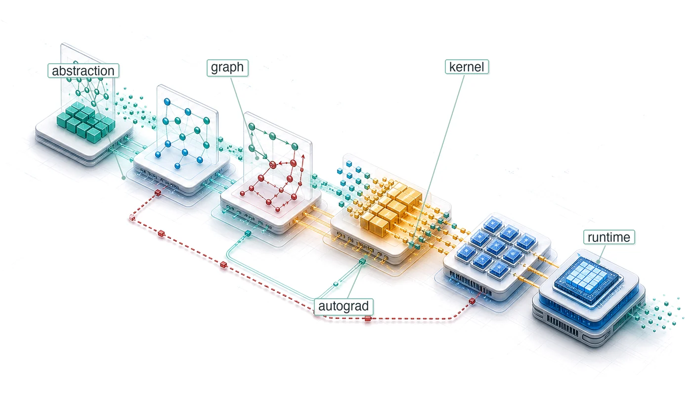
An architecture is a graph of commitments: a transformer commits the system to attention, matrix multiplications, activation state, and memory traffic. The framework is the layer that turns that graph into work the machine can execute. A few calls such as logits = model(tokens), loss = criterion(logits, targets), and loss.backward() hide billions of floating-point operations across memory hierarchies, gradients through millions of parameters via automatic differentiation, thousands of GPU kernel launches, and gigabytes of intermediate state. The API looks simple because the framework is acting as a compiler for the silicon contract.
Architectures specify what computations neural networks perform, but knowing what to compute is entirely different from knowing how to compute it efficiently. A transformer’s attention mechanism requires coordinating computation across memory hierarchies and accelerator cores in patterns that naive implementations would execute 100\(\times\) slower than optimized ones. Implementing these operations from scratch for every model would make deep learning economically infeasible. ML frameworks exist to bridge this gap by lowering abstract model graphs into hardware-aligned execution pipelines that extract maximum performance from silicon.
A framework is to machine learning what a compiler is to traditional programming. A C compiler translates human-readable code into optimized machine instructions, managing register allocation, instruction scheduling, and memory layout. An ML framework translates high-level model definitions into hardware-specific execution plans, managing operator fusion, memory reuse, and device placement. This analogy is more than metaphor: modern frameworks literally include compilers.
Every ML framework, regardless of API or design philosophy, must solve three core problems. The first is the execution problem: deciding when and how computation runs. A framework can execute operations immediately as written (eager execution1) or build a complete description first—a computational graph2 (a structured representation of operations and their dependencies)—and optimize before executing (graph execution). This choice shapes debugging capability, optimization potential, and deployment flexibility.
1 Eager execution: This mode executes each operation immediately, which enables direct debugging with standard tools but sacrifices the global view needed for graph-level optimizations. Without capturing a larger region of computation, an eager runtime cannot fuse across that region or preplan its memory, leaving workload-dependent optimization opportunities for compilers such as torch.compile.
2 Computational graph: The “optimize before executing” distinction in the triggering sentence is the key design choice. Capturing the program as a data structure lets a framework fuse compatible operations into fewer GPU kernels before execution, reducing launch overhead and intermediate memory traffic. The engineering cost of this visibility is that the executed program differs from the source code, making debugging harder, a trade-off every graph-based framework must justify against the performance gain.
Once execution has a shape, the framework must solve the differentiation problem: computing gradients automatically. As established in Neural Computation, training requires derivatives of a loss function with respect to millions or billions of parameters, and manual differentiation is error-prone at this scale. Frameworks therefore apply registered derivative rules across supported operation compositions while managing floating-point arithmetic and the memory overhead of saved values.
The third problem is hardware abstraction: targeting diverse hardware from a single interface. The same model definition should be expressible across CPUs, GPUs, Tensor Processing Units (TPUs), and mobile devices, even though each target has different memory constraints and optimal execution patterns. Within the GPU slice of this problem, some framework ecosystems expose custom-kernel languages so advanced users can write high-performance kernels without dropping all the way to low-level CUDA (Tillet et al. 2019).
Tillet, Philippe, H. T. Kung, and David Cox. 2019. “Triton: An Intermediate Language and Compiler for Tiled Neural Network Computations.” Proceedings of the 3rd ACM SIGPLAN International Workshop on Machine Learning and Programming Languages, 10–19. https://doi.org/10.1145/3315508.3329973.
These three problems are deeply interconnected. The execution model determines when differentiation occurs and what optimizations are possible. The abstraction layer must support both execution styles across all hardware targets. Solving any one problem in isolation leads to frameworks that excel in narrow contexts but fail in broader deployment. Because these problems are ultimately about translating mathematics into efficient hardware execution, a useful perspective is to view frameworks not as libraries but as compilers.
Systems Perspective 1.1: The ML compiler
In the context of the iron law (Iron Law of ML Systems), a framework is a compiler for the silicon contract.
The “source code” is the model architecture (the \(O\) term). The framework’s job is to take this high-level math and compile it into a series of hardware-specific kernel launches that:
- Minimize data movement \((D_{\text{vol}})\) through techniques like kernel fusion.
- Maximize utilization \((\eta_{\text{hw}})\) by matching operations to specialized hardware units like Tensor Cores.
- Minimize overhead \((L_{\text{lat}})\) through efficient asynchronous dispatch and graph capture.
Choosing a framework means choosing the compiler that determines how efficiently a model uses hardware; precision matters: a definition that captures all three responsibilities separates genuine frameworks from numerical libraries that address only one.
Definition 1.1: Machine learning frameworks
Machine learning frameworks are software systems that translate high-level mathematical model definitions into hardware-optimized execution plans by managing the computational graph, automatic differentiation, kernel dispatch, and memory allocation across the hardware hierarchy.
- Significance: Frameworks directly determine the system efficiency \((\eta_{\text{hw}})\) term in the iron law. Compiler-backed operator fusion, for example, can eliminate writes and subsequent reads of intermediate values between compatible operations. Fusing a matrix multiplication, bias add, and rectified linear unit (ReLU) changes how the same mathematics reaches hardware without changing the model.
- Distinction: Unlike a numerical library such as NumPy, which normally evaluates each operation as it is called, an ML framework can capture or defer execution to analyze a larger computational graph and apply cross-operation optimizations: operator fusion, memory layout transformations, and parallel scheduling. Those optimizations require visibility beyond separately dispatched operations.
- Common pitfall: A frequent misconception is that frameworks are interchangeable API wrappers. Framework choice determines which compiler paths are available. PyTorch can recover graph-level optimization from eager code through
torch.compile(), while TensorFlow and JAX commonly rely on XLA-backed compilation paths that lower operations to target hardware. Moving from eager execution to a compiler path can change throughput materially, but the gain depends on model structure, shapes, operator support, and hardware.
The compiler metaphor is not decorative. An ML framework translates logical intent into physical execution under the constraints of the iron law, deciding how to partition computation across memory hierarchies, when to trade numerical precision for throughput, and how to schedule operations so that the dominant term (data movement, computation, or overhead) is minimized. The framework is where the governing physics developed throughout this book becomes executable code.
The scale of this translation is not obvious from the API surface. A single call to loss.backward() triggers operation recording, memory allocation for gradients, reverse-order graph traversal, and hardware-optimized kernel dispatch—machinery that would require hundreds of lines of manual calculus for even a three-layer network. For a contemporary language model, the framework additionally orchestrates billions of floating-point operations across accelerators, coordinating memory hierarchies, numerical precision, and, when the system grows beyond one device, communication libraries. Building this from scratch would be economically prohibitive for most organizations, which is why the history of ML frameworks is a history of progressively automating these layers.
The three problems—execution, differentiation, and abstraction—did not emerge simultaneously. Each arose as a response to scaling limitations in the previous generation of tools. Tracing this evolution explains why modern frameworks are designed as they are and why they embody these particular trade-offs.
Self-Check: Question
A team reports that their model executes correctly on CPU but produces mismatched tensor shapes and silent numerical corruption when switched to a GPU backend because some operators silently default to a different memory layout (such as NCHW versus NHWC). Which of the three fundamental framework problems does this failure most directly expose?
- The hardware abstraction problem, because one unified model interface must preserve consistent semantic behavior, memory layouts, and numerical contracts across diverse hardware backends
- The execution problem, because the operators were evaluated eagerly instead of being captured into a static graph
- The differentiation problem, because the backward pass failed to propagate gradients through non-contiguous strides
- A data engineering pipeline defect unrelated to framework runtime responsibilities
Explain how viewing an ML framework as a compiler for the silicon contract—rather than merely a numerical library like NumPy—changes an engineer’s expectations regarding framework selection and optimization under the systems iron law.
True or False: Two frameworks that expose nearly identical user-facing Python tensor APIs and target the same GPU hardware will necessarily provide equivalent graph-level operator fusion and ahead-of-time compilation capabilities.
An engineering organization chose a specialized research framework for rapid prototyping, only to discover later that the framework lacks export paths to their production edge accelerators, requiring months of manual re-implementation. Applying the chapter’s infrastructure-commitment principle, what is the key systems insight?
- Framework choice is easily reversible because weight arrays can be loaded into any runtime with zero engineering overhead
- Framework selection functions as a durable infrastructure commitment whose reversal cost compounds across model checkpoints, serving runtimes, CI/CD pipelines, and hardware access
- The primary failure was selecting an overly compact model architecture that failed to saturate edge accelerator memory
- Hardware abstraction layers eliminate all differences between training frameworks and production inference engines
The Ladder of Abstraction
In 1979, writing a matrix multiplication in Fortran that used the hardware efficiently required deep knowledge of cache lines, register scheduling, and vector units. By 2016, a single line of Python (torch.matmul(A, W)) could dispatch to a highly optimized implementation without the programmer knowing the details of the silicon. That compression of effort did not happen in one step; it accumulated across four decades of abstraction, each layer solving a bottleneck that made the previous generation impractical for scaling. The result is a ladder of abstraction where each rung automates what the rung below exposed.
- Solving Performance (1979–1992): The original Basic linear algebra subprograms (BLAS)3 standardized reusable low-level linear-algebra primitives (Lawson et al. 1979), while LAPACK4 (Bai et al. 2006) built higher-level numerical routines on top of that foundation. Together, these libraries solved the problem of hardware primitives: stable interfaces let frameworks delegate operations such as
C = A @ B5 to specialized implementations instead of hand-writing silicon-specific code. - Solving Usability (2005–2006): NumPy6 solved the problem of developer velocity. By wrapping low-level BLAS routines in high-level Python (Harris et al. 2020), it allowed scientists to write code in a friendly language while executing it in optimized C/Fortran. This “Vectorization” pattern, where the slow language handles logic and the fast language handles loops, became a durable contract for scientific computing. Jupyter notebooks later extended this usability layer into readable, executable computational workflows for combining code, results, and explanations (Kluyver et al. 2016).
- Solving Differentiation (2007–present): Deep learning frameworks (Theano,7 TensorFlow (Abadi et al. 2016), PyTorch (Paszke et al. 2019)) solved the problem of gradient computation. While NumPy required manual derivation of backpropagation gradients (error-prone and slow), these frameworks made automatic differentiation through computational graphs a standard capability. This turned the chain rule into a software primitive, allowing researchers to define forward passes and get backward passes automatically.
3 BLAS (basic linear algebra subprograms): The 1979 API specification that forms the bottom rung of the ladder described here; it standardized a fixed set of Fortran-callable vector operations, separating the public routine names from the machine-specific implementation decisions beneath them. Every framework above it inherits the broader version of this bargain: call a standard linear-algebra primitive from any language and let a tuned vendor library target the silicon. For modern general matrix multiply (GEMM) on NVIDIA GPUs, that tuned path is cuBLAS rather than the 1979 BLAS specification itself (NVIDIA 2024a).
NVIDIA. 2024a. cuBLAS: CUDA Basic Linear Algebra Subprograms.
Lawson, Charles L., Richard J. Hanson, David R. Kincaid, and Fred T. Krogh. 1979. “Basic Linear Algebra Subprograms for Fortran Usage.” ACM Transactions on Mathematical Software 5 (3): 308–23. https://doi.org/10.1145/355841.355847.
4 LAPACK (linear algebra package): Extends BLAS by providing a standard API for higher-level routines (SVD, eigendecomposition, least-squares) that vendors implement with chip-specific code layered on top of fast GEMM kernels. This layered design is the architectural pattern every ML framework inherits: high-level operations delegate downward to hand-tuned primitives, so a vendor-optimized LAPACK call can execute over 10\(\times\) faster than a naive implementation without the framework author writing a single line of hardware-specific code.
Bai, Zhaojun, James Demmel, Jack Dongarra, Julien Langou, and Jenny Wang. 2006. “LAPACK.” In Handbook of Linear Algebra. Chapman; Hall/CRC. https://doi.org/10.1201/9781420010572-75.
5 GEMM: The matrix-matrix primitive behind C = A @ B. Hardware vendors hand-tune GEMM for their specific chips because dense layers, attention projections, and convolution lowering all rely on matrix multiplication, making this one routine a performance floor for many frameworks above it on the ladder. Its high arithmetic intensity makes GEMM the operation most able to approach peak compute throughput, while small or misaligned shapes often fall back to much lower utilization.
6 NumPy (numerical Python): In 2005, Travis Oliphant unified two competing Python array libraries (Numeric and Numarray) into a single package, giving the scientific computing community one BLAS-backed array standard at the moment it needed to scale. The “vectorization” contract this created (write logic in Python, execute loops in C/Fortran via BLAS) became the design template for every ML framework that followed: PyTorch tensors and TensorFlow arrays are direct descendants, extending the same \(n\)-dimensional array abstraction to GPUs. Python’s role in ML infrastructure inherits much of its shape from this consolidation decision.
Harris, Charles R., K. Jarrod Millman, Stéfan J. van der Walt, Ralf Gommers, Pauli Virtanen, David Cournapeau, Eric Wieser, et al. 2020. “Array Programming with NumPy.” Nature 585 (7825): 357–62. https://doi.org/10.1038/s41586-020-2649-2.
Kluyver, Thomas, Benjamin Ragan-Kelley, Fernando Pérez, Brian Granger, Matthias Bussonnier, Jonathan Frederic, Kyle Kelley, et al. 2016. “Jupyter Notebooks – a Publishing Format for Reproducible Computational Workflows.” In Positioning and Power in Academic Publishing: Players, Agents and Agendas, edited by Fernando Loizides and Birgit Schmidt. IOS Press. https://doi.org/10.3233/978-1-61499-649-1-87.
7 Theano: Developed at the Montreal Institute for Learning Algorithms (MILA) under Yoshua Bengio starting in 2007, Theano was an early and influential Python framework that compiled symbolic mathematical expressions into optimized CPU and GPU code via computational graphs (Bergstra et al. 2010; Team et al. 2016). It demonstrated that a Python-defined computation graph could be compiled for GPU execution without requiring the researcher to write CUDA code. Mila ended active development of Theano in 2017 (Mila 2026).
Bergstra, James, Olivier Breuleux, Frédéric Bastien, Pascal Lamblin, Razvan Pascanu, Guillaume Desjardins, Joseph Turian, David Warde-Farley, and Yoshua Bengio. 2010. “Theano: A CPU and GPU Math Compiler in Python.” Proceedings of the Python in Science Conference 4: 18–24. https://doi.org/10.25080/majora-92bf1922-003.
Team, The Theano Development, Rami Al-Rfou, Guillaume Alain, Amjad Almahairi, Christof Angermueller, Dzmitry Bahdanau, Nicolas Ballas, et al. 2016. “Theano: A Python Framework for Fast Computation of Mathematical Expressions.” arXiv Preprint.
Mila. 2026. Open Source Software.
Machine learning frameworks evolved by progressively abstracting hardware execution details into higher-level API primitives. Frameworks bridge the gap between mathematical intent and silicon reality (figure 1), moving numerical software up the ladder from low-level linear algebra routines to compiled graph execution engines.
\begin{tikzpicture}[node distance=1mm,outer sep=0pt,font=\small\sffamily]
\tikzset{%
    Line/.style={line width=1.0pt,black!50
},
  Box/.style={inner xsep=1pt,
    draw=none,
    fill=#1,
    anchor=west,
    text width=27mm,align=flush center,
    minimum width=28mm, minimum height=13mm
  },
  Box/.default=red
}
\definecolor{col1}{RGB}{128, 179, 255}
\definecolor{col2}{RGB}{255, 255, 128}
\definecolor{col3}{RGB}{204, 255, 204}
\definecolor{col4}{RGB}{230, 179, 255}
\definecolor{col5}{RGB}{255, 153, 204}
\definecolor{col6}{RGB}{245, 82, 102}
\definecolor{col7}{RGB}{255, 102, 102}

\node[Box={col1}](B1){1979};
\node[Box={col2!},right=of B1](B2){1992};
\node[Box={col3},right=of B2](B3){2006};
\node[Box={col4},right=of B3](B4){2007};
\node[Box={col5},right=of B4](B5){2015};
\node[Box={col6},right=of B5](B6){2016};
\node[Box={col7},right=of B6](B7){2018};
%%
\foreach \x in{1,2,...,7}
\draw[dashed,thick,-latex](B\x)--++(270:4.1);

\path[red]([yshift=-7mm]B1.south west)coordinate(P)-|coordinate(K)(B7.south east);

\draw[line width=2pt,-latex](P)--(K)--++(0:3mm);

\def\vi{1.4}
\node[Box={col1!50},below=\vi of B1](BB1){BLAS introduced};
\node[Box={col2!50},below=\vi of B2](BB2){LAPACK extends BLAS};
\node[Box={col3!50},below=\vi of B3](BB3){NumPy becomes Python's numerical backbone};
\node[Box={col4!50},below=\vi of B4](BB4){Theano introduces computational graphs};
\node[Box={col5!50},below=\vi of B5](BB5){TensorFlow popularizes static graphs};
\node[Box={col6!50},below=\vi of B6](BB6){PyTorch introduces dynamic graphs};
\node[Box={col7!50},below=\vi of B7](BB7){JAX introduces functional paradigms};
\end{tikzpicture}Each generation abstracted away details that consumed engineering effort in the previous one, yet each abstraction introduced new trade-offs. BLAS hid assembly-level optimization but fixed the interface. NumPy hid memory management but required manual differentiation. Modern frameworks hide gradient computation but introduce a choice among execution models. The deeper pattern is that every abstraction hides details by preserving a contract about shape, dtype, device, and sometimes units; when that contract becomes implicit, correct components can still compose into a wrong system.
With that contract risk in view, modern frameworks converge on the same three core problems: how to execute computation, how to differentiate it, and how to abstract across hardware. The execution problem comes first because its resolution determines what optimizations the other two problems can exploit.
War Story 1.1: The interface that forgot its units (1999)
Context: NASA’s Mars Climate Orbiter depended on ground software, spacecraft software, navigation teams, and contractor interfaces all agreeing on the physical meaning of exchanged values (Mars Climate Orbiter Mishap Investigation Board 1999).
Mechanism: Ground software supplied by Lockheed Martin computed thruster impulse in English units (pound-force seconds), while JPL navigation software consumed the values assuming SI units (newton-seconds)—a 4.45\(\times\) implicit unit mismatch.
Impact: On September 23, 1999, the spacecraft was lost after entering occultation. Its corrected 57 km periapsis, rather than the planned 226 km, was judged too low for survival.
Response: The board recommended unit-consistency checks, specification audits of transferred data, and stronger end-to-end verification of ground software.
Systems lesson: Framework abstractions are valuable because they carry contracts: shape, dtype, device placement, and physical units. If those contracts are implicit, two pieces of correct code can still compose into a wrong system. ML frameworks hit this whenever tensor memory layouts (such as NCHW vs. NHWC), quantization scale factors, or physical feature units differ across pipeline stages, producing plausible outputs that quietly corrupt downstream inference.
Mars Climate Orbiter Mishap Investigation Board. 1999. Mars Climate Orbiter Mishap Investigation Board Phase i Report. National Aeronautics; Space Administration.
Self-Check: Question
While NumPy provided high-performance linear algebra by wrapping BLAS in Python, what critical scaling bottleneck did it leave unaddressed that motivated the development of deep learning frameworks such as Theano, TensorFlow, and PyTorch?
- Inability to execute matrix multiplications on single-core CPU architectures
- Lack of an \(n\)-dimensional array data structure in scientific computing
- The requirement for manual gradient derivation and hand-written backpropagation passes for multi-layer neural networks
- Inability to run compiled Fortran and C routines through high-level scripting languages
Explain why the relationship between rungs on the ladder of abstraction (such as BLAS/LAPACK, NumPy, and modern deep learning frameworks) is characterized by inheritance rather than replacement.
Order the following historical computing milestones in the evolution of numerical and machine learning software abstractions, from earliest (1979) to most recent (2018):
JAX introduces functional composable transformations and XLA compilation
BLAS standardizes reusable low-level linear algebra primitives
Theano introduces compiled Python computational graphs for GPUs
NumPy establishes Python’s unified \(n\)-dimensional array and vectorization standard
PyTorch introduces dynamic define-by-run execution graphs
LAPACK extends BLAS with higher-level numerical routines (e.g., SVD, factorizations)
The architectural design pattern established by NumPy, where high-level control logic is written in an expressive interpreted language (such as Python) while inner numerical loops are delegated to compiled C/Fortran libraries, is known as ____.
Execution Problem
Consider two engineers writing the same neural network. The first debugs interactively, printing tensor shapes after each operation, inspecting intermediate values, and stepping through code with pdb. The second waits 30 seconds for compilation, then watches the model run 3\(\times\) faster while losing that direct, line-by-line view of intermediate state. Both are correct; they have made different choices about the execution problem, the question of whether operations should execute immediately as written or be recorded for later execution. This choice creates a cascade of engineering trade-offs that shape every aspect of framework behavior, from debugging workflows to deployment options to peak hardware utilization.
Why execution strategy matters: The memory wall
To understand why execution strategy matters so much, return to the widening compute-bandwidth gap quantified by the memory-wall equation (equation). Processor arithmetic has grown faster than memory bandwidth, creating the memory wall. Modern accelerators can perform arithmetic far faster than they can fetch data. Element-wise operations like ReLU use only a tiny fraction of peak compute capacity, not because the hardware is slow, but because they spend nearly all their time waiting for data. The Roofline model formalizes this trade-off, showing exactly when operations are memory bound vs. compute bound.
The memory wall classifies operations as either compute-bound (limited by arithmetic throughput) or memory-bound (limited by data movement). Most individual neural network operation types (activations, normalizations, element-wise operations) are memory bound, though the large matrix multiplications that dominate total compute time can be compute bound.
The key optimization for memory-bound operations is kernel fusion, combining multiple operations into a single GPU function (called a kernel)8 to avoid intermediate memory traffic. Fusing a sequence of normalization, dropout, and activation operations into one kernel can yield large speedups by eliminating intermediate writes between operations. Attention kernels9 use the same principle at larger scale: instead of materializing the full attention matrix in high-bandwidth memory (HBM), a fused implementation can keep tiles close to the compute units, cut HBM accesses by up to 9\(\times\), and produce workload-specific speedups from 15 percent to 3\(\times\) (Dao et al. 2022).
8 Kernel (GPU): In GPU programming, a kernel is the function dispatched to execute in parallel across thousands of threads. Each kernel launch incurs 5–20 \(\mu\)s of CPU-side overhead for parameter assembly and GPU signaling, which means that small, unfused operations spend more time on launch overhead \((L_{\text{lat}})\) than on useful arithmetic. Reducing kernel count through fusion is therefore a direct attack on the overhead term of the iron law.
9 Fused attention kernel: A fused attention kernel combines the \(\mathbf{Q}\mathbf{K}^T\) product, softmax, and value-weighted output into a tiled implementation that keeps intermediate values in on-chip memory rather than materializing the full attention matrix in HBM. FlashAttention is the canonical named example introduced in Network Architectures and reports up to 9\(\times\) fewer HBM accesses with workload-specific speedups from 15 percent to 3\(\times\) (Dao et al. 2022). The framework lesson is broader than the specific algorithm: fusion can shift an operation’s position on the Roofline Model from bandwidth-limited toward throughput-limited execution by reducing round-trips through external memory.
Dao, T., D. Y. Fu, S. Ermon, A. Rudra, and C. Ré. 2022. “FlashAttention: Fast and Memory-Efficient Exact Attention with IO-Awareness.” Advances in Neural Information Processing Systems (NeurIPS) 35: 16344–59. https://doi.org/10.52202/068431-1189.
Frameworks can fuse only operations visible together. Separately dispatched eager operations hide cross-operation opportunities, but graph capture can expose them. A deferred graph lets the framework optimize the captured computation. Execution strategy therefore determines which optimizations are possible and their scope.
The computational graph
Kernel fusion is the key optimization for memory-bound operations, but fusion requires seeing multiple operations together. Frameworks make this visibility possible through the computational graph, a directed acyclic graph (DAG) where nodes represent operations and edges represent data dependencies. This graph is the framework’s internal model of the computation.
Mathematical operations can be decoupled from physical execution through graph representations. The computational graph (figure 2) grounds this abstraction: tensor variables map to data nodes while operations map to transformation nodes.
\begin{tikzpicture}[font=\sffamily\small]
%
\tikzset{%
    Line/.style={line width=1.0pt,black!50,rounded corners
},
  Box/.style={align=flush center,
   shape=circle,
    inner xsep=1pt,
    node distance=1.4,
    draw=BlueLine,
    line width=0.75pt,
    fill=BlueL,
    minimum width=8mm,
  },
}
\node[Box,fill=GreenFill,draw=GreenLine,minimum width=15mm, ](B1){$f(x,y)$};
\node[Box,right=of B1,fill=GreenFill,draw=GreenLine](B2){$z$};
\node[Box,above left=-0.10 and 2 of B1,fill=GreenFill,draw=GreenLine](B3){$x$};
\node[Box,below left=-0.10 and 2 of B1,fill=GreenFill,draw=GreenLine](B4){y};
\draw[-latex,Line](B1)--(B2);
\draw[-latex,Line](B3)to[bend left=25](B1);
\draw[-latex,Line](B4)to[bend right=25](B1);
\end{tikzpicture}Real machine learning models require much more complex graph structures. Figure 3 extends this representation to show a neural network computation graph alongside the system components that reason about it. In the left panel, notice how data flows through six operation nodes in a directed acyclic graph—each node’s output becomes the next node’s input. The right panel reveals what the framework gains from this explicit graph structure: it can query the structure to plan memory allocation for each tensor’s lifetime, and it can assign operations to devices based on data dependencies rather than execution order. The critical insight is that the graph exists independently of execution, enabling the framework to optimize before any arithmetic occurs.
\scalebox{0.9}{%
\begin{tikzpicture}[font=\sffamily\small]

\tikzset{
  Box/.style={ inner xsep=2pt,
    node distance=1.4,
    draw=none,
    line width=0.5pt,,
    fill=none,
    minimum width=27mm, minimum height=15mm
  },
    LineA/.style={violet!40,line width=5pt,{-{Triangle[width=1.0*11pt,length=1.0*8pt]}},shorten <=1pt,shorten >=1pt},
    graphpanel/.style={
        draw=olive!60!black,
        fill=olive!02,
        line width=0.9pt,
        rounded corners=4pt,
        inner sep=14pt,yshift=9pt
    },
    syspanel/.style={
        draw=orange!70!black,
        fill=orange!03,
        line width=0.9pt,
        rounded corners=4pt,
        inner sep=10pt
    },
    opnode/.style={
        circle,node distance=6mm,
        draw=BlueLine,,
        fill=cyan!15,
        minimum size=5mm,
        line width=0.9pt
    },
    compbox/.style={
        draw=orange!80!black,
        fill=orange!12,
        rounded corners=2pt,
        minimum width=2.7cm,
        minimum height=0.9cm,
        align=center,
        line width=0.8pt
    },
    flow/.style={
        -{Latex[length=2.2mm]},
        draw=BrownLine!75,
        line width=0.9pt
    },
}
%CPU style
\tikzset{
pics/cpu/.style = {
        code = {
        \pgfkeys{/channel/.cd, #1}
\begin{scope}[local bounding box = CPU,shift={($(0,0)+(0,0)$)},scale=\scalefac,every node/.append style={transform shape}]
\node[fill=\filllcolor,minimum width=66, minimum height=66,
            rounded corners=2,outer sep=2pt] (C1) {};
\node[fill=white,minimum width=54, minimum height=54] (C2) {};
\node[fill=\filllcolor!50,minimum width=44, minimum height=44] (C3) {\Large\bfseries GPU};

\foreach \x/\y in {0.11/1,0.26/2,0.41/3,0.56/4,0.71/5,0.85/6}{
\node[fill=\filllcolor,minimum width=4, minimum height=15,
           inner sep=0pt,anchor=south](GO\y)at($(C1.north west)!\x!(C1.north east)$){};
}
\foreach \x/\y in {0.11/1,0.26/2,0.41/3,0.56/4,0.71/5,0.85/6}{
\node[fill=\filllcolor,minimum width=4, minimum height=15,
           inner sep=0pt,anchor=north](DO\y)at($(C1.south west)!\x!(C1.south east)$){};
}
\foreach \x/\y in {0.11/1,0.26/2,0.41/3,0.56/4,0.71/5,0.85/6}{
\node[fill=\filllcolor,minimum width=15, minimum height=4,
           inner sep=0pt,anchor=east](LE\y)at($(C1.north west)!\x!(C1.south west)$){};
}
\foreach \x/\y in {0.11/1,0.26/2,0.41/3,0.56/4,0.71/5,0.85/6}{
\node[fill=\filllcolor,minimum width=15, minimum height=4,
           inner sep=0pt,anchor=west](DE\y)at($(C1.north east)!\x!(C1.south east)$){};
}
\end{scope}
    }
  }
}
\tikzset{
pics/dram/.style = {
        code = {
        \pgfkeys{/channel/.cd, #1}
\begin{scope}[shift={($(0,0)+(0,0)$)},scale=\scalefac,every node/.append style={transform shape}]
\node[draw=\drawcolor,fill=\filllcolor!70,line width=1.5*\Linewidth,inner sep=0pt,outer sep=0pt,
minimum width=56mm,minimum height=14mm](DRAM\picname)at(0,0){};
\node[draw=\drawcolor,fill=\filllcolor!30,line width=1.5*\Linewidth,inner sep=0pt,outer sep=0pt,anchor=north,
minimum width=52mm,minimum height=6mm](MDRAM\picname)at(DRAM\picname.south){};
%
\pgfmathsetmacro{\spacing}{56/(6+1)}
\foreach \i in {1,...,6} {
  \pgfmathsetmacro{\x}{\i * \spacing}
  \node[draw=\drawcolor,fill=\filllcolor!20,line width=\Linewidth, inner sep=0pt, outer sep=0pt,
        minimum width=6mm, minimum height=8mm]
        at ([xshift=\x mm]DRAM\picname.west) {};
}
%
\foreach \i in {1,...,19} {
  \pgfmathsetmacro{\x}{\i*(52/20)}
  \draw[draw=\drawcolor, line width=3*\Linewidth]
    ([xshift=\x mm,yshift=1pt]MDRAM\picname.south west) -- ++(0,2mm);
}
\end{scope}
    }
  }
}
\pgfkeys{
  /channel/.cd,
   Depth/.store in=\Depth,
  Height/.store in=\Height,
  Width/.store in=\Width,
  filllcirclecolor/.store in=\filllcirclecolor,
  filllcolor/.store in=\filllcolor,
  drawcolor/.store in=\drawcolor,
  drawcircle/.store in=\drawcircle,
  scalefac/.store in=\scalefac,
  Linewidth/.store in=\Linewidth,
  picname/.store in=\picname,
  filllcolor=BrownLine,
  filllcirclecolor=cyan!40,
  drawcolor=black,
  drawcircle=violet,
  scalefac=1,
  Linewidth=0.5pt,
  Depth=1.3,
  Height=0.8,
  Width=1.1,
  picname=C
}

    % graph nodes
    \node[opnode] (a)  {};
    \node[opnode,below left=of a] (b) {};
    \node[opnode,below right =of a] (c) {};
    \node[opnode,below=of b] (d)  {};
    \node[opnode,below =of c] (e) {};
    \node[opnode,below right=of d] (f) {};
    % edges
    \draw[flow] (a) -- (b);
    \draw[flow] (a) -- (c);
    \draw[flow] (b) -- (d);
    \draw[flow] (c) -- (e);
    \draw[flow] (d) -- (f);
    \draw[flow] (e) -- (f);
    % optional cross-edge
    \draw[flow] (b) -- (e);

    \node[opnode,minimum size=3mm,below left= 0.33 and 1.65of f] (l) {};
    \node[right=0pt of l,font=\sffamily\footnotesize](O){Operations};
    \draw[flow]($(O.east)+(1mm,0)$)--++(0:7mm)coordinate(A);
    \node[right=0pt of A,font=\sffamily\footnotesize](AA){Data flow};
    \scoped[on background layer]
    \node[graphpanel,fit=(a)(l)(O)(AA),inner xsep=6pt](FF){};
    \node[below=1pt of FF.north,font=\sffamily\bfseries\footnotesize]{Computational Graph};
%
   \node[right=29mm of FF.27,Box](MM){};
   \node[below=-6pt of MM](T1){Memory Management};
   \pic[shift={(0,0.1)}] at  (MM){dram={scalefac=0.43,picname=1,
   drawcolor=black,filllcolor=OrangeLine!50!,Linewidth=0.5pt}};
   \node[right=29mm of FF.338,Box](DP){};
      \node[below=1pt of DP](T2){Device Placement};
   \pic[shift={(0,0)}] at (DP) {cpu={scalefac=0.45,picname=1,
   drawcolor=RedLine,filllcolor=BlueLine!80!,Linewidth=0.5pt}};

   \scoped[on background layer]
   \node[fit=(MM)(T1)(T2),syspanel,yshift=1.0mm,inner xsep=6pt](DD){};
   \node[below=1pt of DD.north,font=\sffamily\bfseries\footnotesize]{System Components};

\draw[LineA](FF)--
node[above,pos=0.45,text=black!70,font=\sffamily\footnotesize]{Interacts with}
(DD);
\end{tikzpicture}}This graph representation is more than a visualization; it is the data structure that enables both efficient execution and automatic differentiation. The answer to when this graph is constructed creates a design choice with cascading implications across four dimensions. Debugging benefits from visibility into intermediate values and step-through execution. Optimization benefits from seeing multiple operations at once, which enables fusion. Deployment benefits when execution no longer depends on the Python interpreter. Flexibility benefits when control flow can depend on computed tensor values.
No single execution model optimizes all these dimensions. Frameworks must choose their position in this trade-off space, and practitioners must understand these trade-offs to select appropriate tools and write efficient code. The three execution families that follow are different answers to the same systems question: how much graph visibility should the framework trade for immediate execution and debugging?
Three execution strategies
The computational graph representation enables global optimization, but it leaves a critical design choice unresolved: when the framework builds the graph. Consider a simple operation like y = x * 2. One approach performs the multiplication immediately, storing the result in y. This is natural and debuggable, but the framework sees only one operation at a time. The other approach defers execution, recording the intention to multiply and building a graph of operations that runs later when explicitly requested. This is less intuitive, but the framework sees the complete computation, which enables optimization.
Neither approach dominates; each embodies different trade-offs between flexibility and optimization potential. Modern frameworks have explored three primary execution strategies: eager execution with dynamic graphs, static computation graphs, and hybrid approaches that combine just-in-time (JIT) compilation with eager development. Each strategy has distinct systems implications.
Eager execution with dynamic graphs
Eager execution evaluates each operation immediately as the program calls it, building the computation graph dynamically at runtime. A side-by-side comparison shows how this differs from graph-based execution at the code level.
Example 1.1: Eager vs. graph execution code comparison
PyTorch (eager execution):
import torch

x = torch.tensor([1.0, 2.0])
y = x * 2
print(f"Intermediate value: {y}")  # Works immediately
z = y.sum()
TensorFlow 1.x (static graph):
import tensorflow as tf

x = tf.placeholder(tf.float32)
y = x * 2
# print(y) -> Prints Tensor("mul:0"...), not value!
z = tf.reduce_sum(y)

with tf.Session() as sess:
    result = sess.run(z, feed_dict={x: [1.0, 2.0]})
Systems insight: Eager execution exposes intermediate values as ordinary runtime state, which makes debugging direct. Static graphs stage computation before execution, which enables whole-graph optimization but changes the debugging model.
Eager execution runs operations immediately as encountered, building the computation graph dynamically during execution. When a programmer writes y = x * 2, the multiplication happens instantly and the result is available for immediate use.
This provides the flexibility of normal programming: developers can print intermediate values, use conditionals based on computed results, and debug with standard tools. The framework records operations as they happen, constructing a dynamic graph that reflects the actual execution path taken.
For gradient computation, the framework records a history of operations in what is called an autograd tape,10 a transient data structure built during execution. Each tensor operation creates a node that records: the operation performed, references to input tensors, and how to compute gradients. These nodes form a DAG that records the actual path taken during forward-pass execution rather than a graph fixed in advance. Listing 1 shows how PyTorch records operations as they execute in its default eager mode.
10 Autograd tape: A transient data structure built during forward execution, where nodes record operations, dependencies, and backward functions for chain-rule evaluation. Its memory footprint grows with model depth and sequence length as saved activations accumulate until released during backpropagation. For deep models, frameworks retain selected activations and recompute others via activation checkpointing to prevent OOM failures.
import torch

x = torch.tensor([1.0], requires_grad=True)
y = x * 2  # Executes immediately; records MulBackward node
z = y + 1  # Executes immediately; records AddBackward node
# The autograd tape exists NOW, built during execution
After these two operations, the framework has constructed an autograd tape with two nodes: one for the multiplication and one for the addition. The tape records that z depends on y, and y depends on x.
Calling z.backward() traverses this tape in reverse topological order, applying the chain rule at each node:
- Compute \(\frac{\partial z}{\partial z} = 1\) (seed gradient)
- Call
AddBackward0.backward()\(\rightarrow \frac{\partial z}{\partial y} = 1\) - Call
MulBackward0.backward()\(\rightarrow \frac{\partial z}{\partial x} = 2\) - Accumulate gradient in
x.grad
After backward() completes, the autograd graph is normally released. The next forward pass builds a new graph. Values needed for gradients are saved during the forward pass and remain live until backward consumes them, so their memory cost spans both phases rather than appearing only during backward.
Example 1.2: In-place operations can break gradients
Scenario: An engineer applies an in-place mutation (
x += 1) within a custom PyTorch activation function to reduce memory allocations.
Diagnosis: In-place operations overwrite tensor memory containing forward-pass activations required by the autograd tape for backward-pass gradient computation, triggering a runtime version-counter error (PyTorch Contributors 2026a).
Systems lesson: Framework automatic differentiation depends on immutable forward-pass activation records. Unchecked in-place memory mutations break autograd tape dependencies, forcing runtime framework execution halts.
PyTorch Contributors. 2026a. PyTorch Autograd Mechanics.
In eager execution frameworks, operations evaluate imperatively as host code encounters them. Trace the execution loop in figure 4, following the define-and-dispatch sequence that sends individual operations directly to device stream queues.
\begin{tikzpicture}[line join=round,font=\sffamily\small]
\tikzset{%
  Line/.style={line width=0.75pt,black!50,text=black},
  Box/.style={align=flush center,
    inner xsep=2pt,
    node distance=0.75,
    draw=BlueLine,
    line width=0.75pt,
    fill=BlueL!30,
    %text width=35mm,
    minimum width=35mm, minimum height=11mm
  },
 decision/.style = {Box,diamond,text width=35mm,aspect=1.95, inner xsep=7pt,inner ysep=-2ex, fill=VioletL2!70,
 draw=VioletLine},
  startstop/.style = {Box,minimum width=25mm,  rounded corners=10pt, fill=red!10, draw=RedLine},
  LineA/.style={black!50,line width=1.5pt,{-{Triangle[width=1.0*5pt,length=1.0*5pt]}},shorten <=0pt,shorten >=0pt},
}

\tikzset{
pics/repeat/.style = {
        code = {
        \pgfkeys{/channel/.cd, #1}
\begin{scope}[shift={($(0,0)+(0,0)$)},scale=\scalefac,every node/.append style={transform shape}]
\def\w{4cm}
\def\h{15mm}
\def\r{6mm} % radius
\def\gap{4mm} % break lengths
\draw[\filllcirclecolor, -{Latex[length=10pt,width=15pt]},line width=\Linewidth]
  (\w,\h-\r) -- (\w,\r)
  arc[start angle=0, end angle=-90, radius=\r]
  -- (\gap,0);
%
  \draw[\filllcolor, -{Latex[length=10pt,width=15pt]},line width=\Linewidth]
  (0,\r) -- (0,\h-\r)
  arc[start angle=180, end angle=90, radius=\r]
  -- ({\w-\gap},\h);
\end{scope}
    }
  }
}
\tikzset{
pics/interpreter/.style = {
        code = {
        \pgfkeys{/channel/.cd, #1}
\def\ra{}
\begin{scope}[shift={($(0,0)+(0,0)$)},scale=\scalefac,every node/.append style={transform shape}]
\node[red,font=\Large\bfseries]at(-0.75,0.6){\textless\,/\,\textgreater};
\draw[line cap=round,line join=round,yellow,line width=\Linewidth](-1.15,-0.1)--(-0.95,-0.1);
\draw[line cap=round,line join=round,red,line width=\Linewidth](-0.7,-0.1)--(0.1,-0.1);

\draw[line cap=round,line join=round,yellow,line width=\Linewidth](-1.15,-0.5)--(0,-0.5);

\draw[line cap=round,line join=round,yellow,line width=\Linewidth](-1.15,-0.9)--(-0.75,-0.9);
\draw[line cap=round,line join=round,red,line width=\Linewidth](-0.45,-0.9)--(0.45,-0.9);
\draw[line cap=round,line join=round,cyan,line width=\Linewidth](0.75,-0.9)--(1.1,-0.9);

\draw[line cap=round,line join=round,yellow,line width=\Linewidth](-1.15,-1.3)--(-1,-1.3);
\draw[line cap=round,line join=round,red,line width=\Linewidth](-0.65,-1.3)--(-0.10,-1.3);
\draw[line cap=round,line join=round,cyan,line width=\Linewidth](0.2,-1.3)--(1.1,-1.3);
\end{scope}
    }
  }
}
%CPU
\tikzset{%
 pics/cpu/.style = {
        code = {
        \pgfkeys{/channel/.cd, #1}
\begin{scope}[local bounding box=FUNNEL,scale=\scalefac, every node/.append style={transform shape}]
\node[fill=\filllcolor,minimum width=66, minimum height=66,
            rounded corners=2,outer sep=2pt] (C1) {};
\node[fill=white,minimum width=54, minimum height=54] (C2) {};
\node[fill=\filllcolor!40,minimum width=44, minimum height=44] (C3) {\Large\bfseries GPU};

\foreach \x/\y in {0.11/1,0.26/2,0.41/3,0.56/4,0.71/5,0.85/6}{
\node[fill=\filllcolor,minimum width=3, minimum height=15,
           inner sep=0pt,anchor=south](GO\y)at($(C1.north west)!\x!(C1.north east)$){};
}
\foreach \x/\y in {0.11/1,0.26/2,0.41/3,0.56/4,0.71/5,0.85/6}{
\node[fill=\filllcolor,minimum width=3, minimum height=15,
           inner sep=0pt,anchor=north](DO\y)at($(C1.south west)!\x!(C1.south east)$){};
}
\foreach \x/\y in {0.11/1,0.26/2,0.41/3,0.56/4,0.71/5,0.85/6}{
\node[fill=\filllcolor,minimum width=15, minimum height=3,
           inner sep=0pt,anchor=east](LE\y)at($(C1.north west)!\x!(C1.south west)$){};
}
\foreach \x/\y in {0.11/1,0.26/2,0.41/3,0.56/4,0.71/5,0.85/6}{
\node[fill=\filllcolor,minimum width=15, minimum height=3,
           inner sep=0pt,anchor=west](DE\y)at($(C1.north east)!\x!(C1.south east)$){};
}
 \end{scope}
     }
  }
}
%start
\tikzset{%
 pics/start/.style = {
        code = {
        \pgfkeys{/channel/.cd, #1}
\begin{scope}[local bounding box=START,scale=\scalefac, every node/.append style={transform shape}]
\node[fill=\filllcolor,minimum width=6mm, minimum height=6mm,
            outer sep=2pt] (C1) {};
\node[isosceles triangle,isosceles triangle apex angle=45,xshift=-2.5pt,
    inner sep=1pt, fill=white,minimum size =3.5mm] (T1)at (C1){};
 \end{scope}
     }
  }
}
%check
\tikzset{pics/.cd,
checkmark/.style={code={
        \pgfkeys{/channel/.cd, #1}
\pgfgettransformentries{\tmpxx}{\tmp}{\tmp}{\tmp}{\tmp}{\tmp}
\draw[line width=\tmpxx*1pt,draw=none,fill=\filllcirclecolor,line join=bevel] (0,.35) -- (.25,0) to[bend left=5] (0.8,.6) to[bend
right=5] (.25,.18) -- cycle;}}}
\tikzset{%
 pics/checkI/.style = {
        code = {
        \pgfkeys{/channel/.cd, #1}
\begin{scope}[local bounding box=CHECK,scale=\scalefac, every node/.append style={transform shape}]
\node[fill=\filllcolor,minimum width=6mm, minimum height=6mm,
            outer sep=2pt] (C1) {};
\pic[shift={(-0.27,-0.19)},scale=0.7]{checkmark};
 \end{scope}
     }
  }
}
\pgfkeys{
  /channel/.cd,
   Depth/.store in=\Depth,
  Height/.store in=\Height,
  Width/.store in=\Width,
  filllcirclecolor/.store in=\filllcirclecolor,
  filllcolor/.store in=\filllcolor,
  drawcolor/.store in=\drawcolor,
  drawcircle/.store in=\drawcircle,
  scalefac/.store in=\scalefac,
  Linewidth/.store in=\Linewidth,
  picname/.store in=\picname,
  filllcolor=BrownLine,
  filllcirclecolor=violet!20,
  drawcolor=red,
  drawcircle=violet,
  scalefac=1,
  Linewidth=0.5pt,
  Depth=1.3,
  Height=0.8,
  Width=1.1,
  picname=C
}

\node[startstop](B1){};
\coordinate(GO1)at($(B1.north west)!0.33!(B1.north east)$);
\coordinate(T1)at($(GO1)!0.5!(B1.south east)$);
\node[align=center]at(T1){Start};
\begin{scope}
\coordinate(I1)at($(GO1)!0.5!(B1.south west)$);
\clip (B1.south west) rectangle (GO1);
%\fill[RedLine!30,rounded corners=10pt] (B1.south west) rectangle (B1.north east);
\end{scope}
\draw[dashed,RedLine,  line width=0.75pt,](GO1)--(GO1|-B1.south west);
\node[startstop,fill=none]{};
\pic[shift={(0,0)}] at  (I1){start={scalefac=1,picname=1,filllcolor=GreenLine, Linewidth=0.7pt}};
%Define
\node[Box,right=of B1](B2){};
\node[above=1pt of B2,text=black!70]{Python Dispatch};
\coordinate(GO2)at($(B2.north west)!0.3!(B2.north east)$);
%\fill[fill=BlueL!90](B2.south west)rectangle(GO2);
\coordinate(T2)at($(GO2)!0.5!(B2.south east)$);
\coordinate(I2)at($(GO2)!0.5!(B2.south west)$);
\node[align=center]at(T2){Define\\Operation};
\draw[dashed,BlueLine,  line width=0.75pt,](GO2)--(GO2|-B2.south west);
\node[Box,right=of B1,fill=none]{};
\pic[shift={(0.05,0.11)}] at  (I2){interpreter={scalefac=0.35,picname=1,
filllcolor=cyan!30!, Linewidth=1.5pt,filllcirclecolor=orange}};
 %Execute
\node[Box,right=of B2](B3){};
\node[above=1pt of B3,text=black!70]{GPU Kernel};
\coordinate(GO3)at($(B3.north west)!0.3!(B3.north east)$);
%\fill[fill=BlueL!90](B3.south west)rectangle(GO3);
\coordinate(T3)at($(GO3)!0.5!(B3.south east)$);
\coordinate(I3)at($(GO3)!0.5!(B3.south west)$);
\node[align=center]at(T3){Execute\\Operation};
\draw[dashed,BlueLine,  line width=0.75pt,](GO3)--(GO3|-B3.south west);
\node[Box,right=of B2,fill=none](B3){};
\pic[shift={(0,0)}] at  (I3){cpu={scalefac=0.23,picname=1,filllcolor=BrownLine, Linewidth=0.7pt}};
%More operations
\node[decision,right=of B3](B4){More\\operations?};
\path[red](B4.west)|-coordinate(SR4)(B4.south);
\pic[shift={(-0.30,-0.14)}] at  (SR4){repeat={scalefac=0.3,picname=1,filllcolor=RedLine,
Linewidth=4pt,filllcirclecolor=GreenLine}};
%End
\node[startstop,right=of B4](B5){};
\coordinate(GO5)at($(B5.north west)!0.33!(B5.north east)$);
\coordinate(T5)at($(GO5)!0.5!(B5.south east)$);
\coordinate(I5)at($(GO5)!0.5!(B5.south west)$);
\node[align=center]at(T5){End};
\begin{scope}
\clip (B5.south west) rectangle (GO5);
%\fill[RedLine!30,rounded corners=10pt] (B5.south west) rectangle (B5.north east);
\end{scope}
\draw[dashed,RedLine,  line width=0.75pt,](GO5)--(GO5|-B5.south west);
\node[startstop,right=of B4,fill=none](B5){};
\pic[shift={(0,0)}] at  (I5){checkI={scalefac=1,picname=1,filllcolor=GreenLine, filllcirclecolor=white,Linewidth=0.7pt}};
%arrows
\foreach \i in {1,2,3,4}{
\pgfmathtruncatemacro{\x}{\i + 1}
\draw[LineA](B\i)--coordinate[pos=0.3](SR\i)(B\x);
}
\node[above=0pt of SR4]{No};
\draw[LineA](B4.south)--node[right,pos=0.5]{Yes}++(270:0.55)-|(B2);
\end{tikzpicture}Systems implications: Flexibility
The dynamic autograd tape expresses data-dependent behavior directly in the host language. Conditionals and loops can depend on tensor values computed during execution, enabling algorithms like beam search, dynamic recurrent neural network lengths, or adaptive computation that adjust their behavior based on intermediate results. Static graphs can also represent data-dependent control flow and dynamic dimensions through graph operations, but eager execution makes these patterns natural to write and debug in Python. Because operations are issued immediately, developers can print tensors, inspect values, and use standard debuggers (pdb, breakpoints) to diagnose errors much as they would in another Python program.
Systems implications: Overhead
This flexibility comes with performance costs that map directly to the iron law (Iron Law of ML Systems). Each training forward pass constructs an autograd tape dynamically, adding host-side Python dispatch overhead and graph-recording work to \(L_{\text{lat}}\). Operations pass through the framework dispatcher before device kernels are launched, so overhead becomes significant when individual kernels are short. Eager execution alone also lacks a static globally captured graph, preventing the framework compiler from performing kernel fusion (combining multiple element-wise operations into a single GPU kernel launch to eliminate intermediate HBM reads/writes) or pre-allocating a static memory arena for intermediate activations (\(D_{\text{vol}}\)). The autograd tape retains the values requested by backward rules, adding memory pressure until those values can be released. Together, these costs create a performance ceiling that becomes visible as operations grow smaller and dispatch overhead dominates computation.
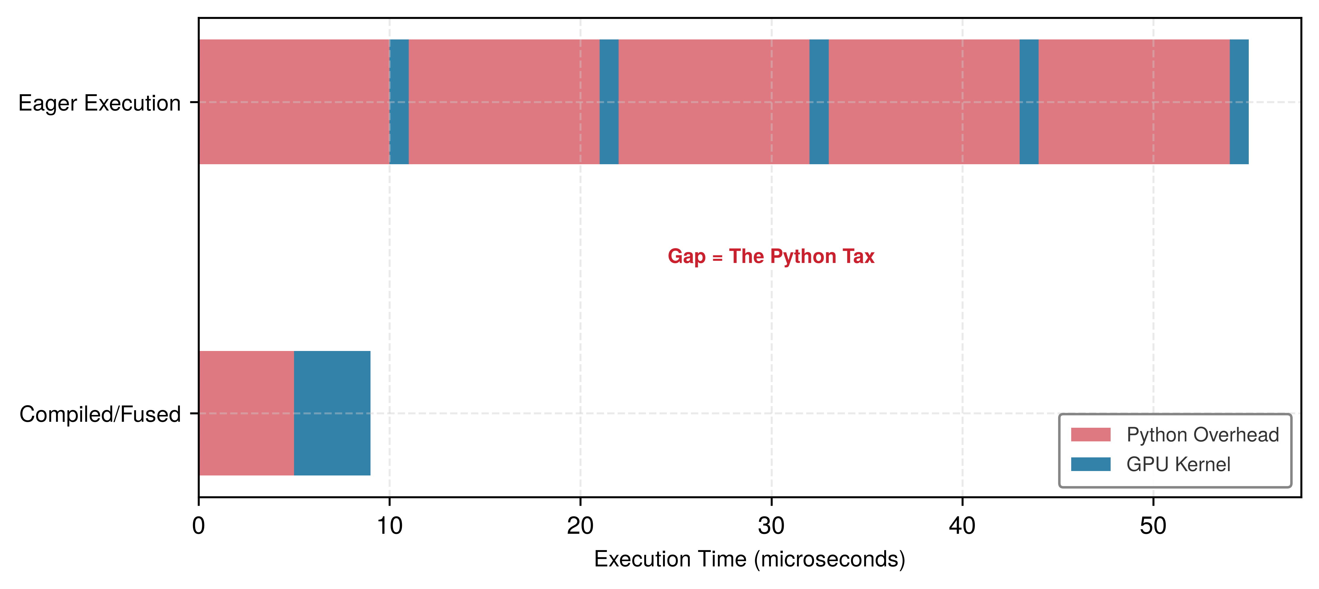
Eager execution’s performance ceiling is driven by a fundamental systems mismatch: the speed of the host-side interpreter vs. the speed of the device-side silicon. The dispatch tax, defined as the fraction of time spent in the host-side orchestration (Python) vs. actual device execution (GPU), quantifies this mismatch.
As work grows, useful compute outpaces fixed dispatch cost; the tax shrinks.
In the illustrative eager-execution model used here, every operation pays a fixed “tax” of approximately 15 \(\mu\)s for host-side dispatch, type checks, and kernel launch. Actual overhead varies by framework, backend, and hardware, but its relative weight still depends on operation size. For a small operation such as a ReLU on a small vector, the kernel might execute in only 1 \(\mu\)s, so the modeled dispatch tax reaches 94 percent and the GPU spends most of its time waiting for the next command. For a large operation such as a large matrix multiply, the kernel executes for 100 \(\mu\)s, the modeled dispatch tax drops to 13 percent, and the system becomes compute bound.
The dispatch tax explains why models with many small layers run significantly slower than their raw FLOP count predicts. Bottleneck diagnostic places this symptom in the bottleneck taxonomy, classifying a dispatch-dominated workload as latency-bound rather than compute-bound and showing which optimizations actually move it. To approach efficient execution, frameworks must move from kernel-by-kernel dispatch to graph-level execution, where the dispatch tax is paid once for the entire graph rather than per operation. The hybrid JIT and compilation strategies in section 1.3.3.3 exist precisely to address this overhead.
The overhead costs of eager execution motivate the opposite design: capturing the entire computation before executing any of it. This is precisely what static computation graphs provide.
Static computation graphs
Static graph execution defines the complete computational graph as a symbolic representation first, then executes it separately. This “define-then-run” execution model means the graph exists before any computation occurs, enabling aggressive ahead-of-time optimization. The key insight is that if the framework sees the entire computation before running it, the framework can analyze, transform, and optimize the graph globally—visibility unavailable across separate eager calls unless a compiler captures them. Operator fusion works through the canonical global transformation this enables: for \(N\) elements of \(b\) bytes each, fusing a chain of \(k\) elementwise operations into one kernel reduces idealized read-and-write traffic from \(2kNb\) to \(2Nb\) bytes.
Two-phase execution
Static graphs implement a clear separation between graph construction and execution. Listing 2 illustrates the two phases using TensorFlow 1.x, which exemplified this approach. It deliberately runs the same x * 2 then + 1 computation shown under eager execution in listing 1, holding the arithmetic fixed so that the only thing that changes is when it executes: symbolic definition creates placeholders and operations without computation, while explicit execution triggers actual arithmetic.
# Phase 1: Graph Construction (symbolic, no computation)
import tensorflow.compat.v1 as tf

tf.disable_v2_behavior()

# Define graph symbolically
x = tf.placeholder(tf.float32, shape=[1])  # Just a placeholder
y = x * 2  # Not executed, just recorded
z = y + 1  # Still no execution
# At this point, nothing has been computed

# Phase 2: Graph Execution (actual computation)
with tf.Session() as sess:
    result = sess.run(z, feed_dict={x: [1.0]})
    # Now computation happens: result = [3.0]
Static graph compilation separates graph construction from tensor execution. Observe the phase division in figure 5, noting how symbolic graph definition on the left precedes ahead-of-time optimization and runtime execution on the right.
\begin{tikzpicture}[line join=round,font=\sffamily\small]
\tikzset{%
  Box/.style={align=flush center,
    inner xsep=2pt,
    node distance=0.65,
    draw=BlueLine,
    line width=0.75pt,
    fill=BlueL!30,
    %text width=35mm,
    minimum width=27mm, minimum height=14mm
  },
  Box2/.style={Box, draw=BrownLine, fill=BrownL!30,
  },
  LineA/.style={black!40,line width=6.5pt,{-{Triangle[width=1.0*12pt,length=1.0*5pt]}},shorten <=0pt,shorten >=0pt},
}

\tikzset{
pics/interpreter/.style = {
        code = {
        \pgfkeys{/channel/.cd, #1}
\def\ra{}
\begin{scope}[shift={($(0,0)+(0,0)$)},scale=\scalefac,every node/.append style={transform shape}]
\node[red,font=\Large\bfseries]at(-0.75,0.6){\textless\,/\,\textgreater};
\draw[line cap=round,line join=round,violet,line width=\Linewidth](-1.15,-0.1)--(-0.95,-0.1);
\draw[line cap=round,line join=round,red,line width=\Linewidth](-0.7,-0.1)--(0.1,-0.1);

\draw[line cap=round,line join=round,violet,line width=\Linewidth](-1.15,-0.5)--(0,-0.5);

\draw[line cap=round,line join=round,violet,line width=\Linewidth](-1.15,-0.9)--(-0.75,-0.9);
\draw[line cap=round,line join=round,red,line width=\Linewidth](-0.45,-0.9)--(0.45,-0.9);
\draw[line cap=round,line join=round,cyan,line width=\Linewidth](0.75,-0.9)--(1.1,-0.9);

\draw[line cap=round,line join=round,violet,line width=\Linewidth](-1.15,-1.3)--(-1,-1.3);
\draw[line cap=round,line join=round,red,line width=\Linewidth](-0.65,-1.3)--(-0.10,-1.3);
\draw[line cap=round,line join=round,cyan,line width=\Linewidth](0.2,-1.3)--(1.1,-1.3);
\end{scope}
    }
  }
}
%CPU
\tikzset{%
 pics/cpu/.style = {
        code = {
        \pgfkeys{/channel/.cd, #1}
\begin{scope}[local bounding box=FUNNEL,scale=\scalefac, every node/.append style={transform shape}]
\node[fill=\filllcolor,minimum width=66, minimum height=66,
            rounded corners=2,outer sep=2pt] (C1) {};
\node[fill=white,minimum width=54, minimum height=54] (C2) {};
\node[fill=\filllcolor!40,minimum width=44, minimum height=44] (C3) {\Large\bfseries GPU};

\foreach \x/\y in {0.11/1,0.26/2,0.41/3,0.56/4,0.71/5,0.85/6}{
\node[fill=\filllcolor,minimum width=3, minimum height=15,
           inner sep=0pt,anchor=south](GO\y)at($(C1.north west)!\x!(C1.north east)$){};
}
\foreach \x/\y in {0.11/1,0.26/2,0.41/3,0.56/4,0.71/5,0.85/6}{
\node[fill=\filllcolor,minimum width=3, minimum height=15,
           inner sep=0pt,anchor=north](DO\y)at($(C1.south west)!\x!(C1.south east)$){};
}
\foreach \x/\y in {0.11/1,0.26/2,0.41/3,0.56/4,0.71/5,0.85/6}{
\node[fill=\filllcolor,minimum width=15, minimum height=3,
           inner sep=0pt,anchor=east](LE\y)at($(C1.north west)!\x!(C1.south west)$){};
}
\foreach \x/\y in {0.11/1,0.26/2,0.41/3,0.56/4,0.71/5,0.85/6}{
\node[fill=\filllcolor,minimum width=15, minimum height=3,
           inner sep=0pt,anchor=west](DE\y)at($(C1.north east)!\x!(C1.south east)$){};
}
 \end{scope}
     }
  }
}
%graph style
\tikzset{
pics/graph3D/.style = {
        code = {
        \pgfkeys{/channel/.cd, #1}
\begin{scope}[local bounding box=GRAPH,scale=1, every node/.append style={transform shape}]
\def\dx{\Width}
\def\dy{\Height}
\def\dz{\Depth}
% koordinata donjeg levog ugla (početak bara)
\def\x{0}
\def\y{0.15}
\def\z{0}
% boje
\draw[draw=\filllcirclecolor,line width=1pt](-0.2,0)--(1.3,0);
\draw[draw=\filllcirclecolor,line width=1pt](-0.2,0)--(-0.2,1.2);
\filldraw[fill=\filllcolor!10, draw=\drawcolor] (\x,\y+\dy,\z) -- (\x,\y+\dy,\z+\dz) -- (\x+\dx,\y+\dy,\z+\dz) -- (\x+\dx,\y+\dy,\z) -- cycle; % gornja strana
\filldraw[fill=\filllcolor!50, draw=\drawcolor] (\x+\dx,\y,\z) -- (\x+\dx,\y,\z+\dz) -- (\x+\dx,\y+\dy,\z+\dz) -- (\x+\dx,\y+\dy,\z) -- cycle; % desna strana
\filldraw[fill=\filllcolor!60, draw=\drawcolor] (\x,\y,\z+\dz) -- (\x+\dx,\y,\z+\dz) -- (\x+\dx,\y+\dy,\z+\dz) -- (\x,\y+\dy,\z+\dz) -- cycle; % prednja strana
\end{scope}
    }
  }
}
\tikzset{mycylinder/.style={cylinder, shape border rotate=90, aspect=1.3, draw, fill=white,
minimum width=25mm,minimum height=11mm,line width=\Linewidth,node distance=-0.15},
pics/data/.style = {
        code = {
        \pgfkeys{/channel/.cd, #1}
\begin{scope}[local bounding box=STREAMING,scale=\scalefac, every node/.append style={transform shape}]
\node[mycylinder,fill=\filllcolor!50] (A) {};
\node[mycylinder, above=of A,fill=\filllcolor!30] (B) {};
\node[mycylinder, above=of B,fill=\filllcolor!10] (C) {};
\fill[\filllcolor!50!black]($(C.west)!0.12!(C.east)$)circle(3pt);
\fill[\filllcolor!50!black]($(B.west)!0.12!(B.east)$)circle(3pt);
\fill[\filllcolor!50!black]($(A.west)!0.12!(A.east)$)circle(3pt);
 \end{scope}
     }
  }
}
\tikzset{pics/brain/.style = {
        code = {
        \pgfkeys{/channel/.cd, #1}
\begin{scope}[local bounding box=BRAIN,scale=\scalefac, every node/.append style={transform shape}]
\fill[fill=\filllcolor!50](0.1,-0.5)to[out=0,in=180](0.33,-0.5)
to[out=0,in=270](0.45,-0.38)to(0.45,-0.18)
to[out=40,in=240](0.57,-0.13)to[out=110,in=310](0.52,-0.05)
to[out=130,in=290](0.44,0.15)to[out=90,in=340,distance=8](0.08,0.69)
to[out=160,in=80](-0.42,-0.15)to (-0.48,-0.7)to(0.07,-0.7)to(0.1,-0.5)
(-0.10,-0.42)to[out=310,in=180](0.1,-0.5);
\draw[draw=\drawcolor,line width=\Linewidth](0.1,-0.5)to[out=0,in=180](0.33,-0.5)
to[out=0,in=270](0.45,-0.38)to(0.45,-0.18)
to[out=40,in=240](0.57,-0.13)to[out=110,in=310](0.52,-0.05)
to[out=130,in=290](0.44,0.15)to[out=90,in=340,distance=8](0.08,0.69)
(-0.42,-0.15)to (-0.48,-0.7)
(0.07,-0.7)to(0.1,-0.5)
(-0.10,-0.42)to[out=310,in=180](0.1,-0.5);
\draw[fill=\filllcolor,line width=\Linewidth](-0.3,-0.10)to(0.08,0.60)
to[out=60,in=50,distance=3](-0.1,0.69)to[out=160,in=80](-0.26,0.59)to[out=170,in=90](-0.46,0.42)
to[out=170,in=110](-0.54,0.25)to[out=210,in=150](-0.54,0.04)
to[out=240,in=130](-0.52,-0.1)to[out=300,in=240]cycle;
\draw[fill=\filllcolor,line width=\Linewidth]
(-0.04,0.64)to[out=120,in=0](-0.1,0.69)(-0.19,0.52)to[out=120,in=330](-0.26,0.59)
(-0.4,0.33)to[out=150,in=280](-0.46,0.42)
%
(-0.44,-0.03)to[bend left=30](-0.34,-0.04)
(-0.33,0.08)to[bend left=40](-0.37,0.2) (-0.37,0.12)to[bend left=40](-0.45,0.14)
(-0.26,0.2)to[bend left=30](-0.24,0.13)
(-0.16,0.32)to[bend right=30](-0.27,0.3)to[bend right=30](-0.29,0.38)
(-0.13,0.49)to[bend left=30](-0.04,0.51);

\draw[rounded corners=0.8pt,\drawcircle,-{Circle[fill=\filllcirclecolor,length=2.5pt]}](-0.23,0.03)--(-0.15,-0.03)--(-0.19,-0.18)--(-0.04,-0.28);
\draw[rounded corners=0.8pt,\drawcircle,-{Circle[fill=\filllcirclecolor,length=2.5pt]}](-0.17,0.13)--(-0.04,0.05)--(-0.06,-0.06)--(0.14,-0.11);
\draw[rounded corners=0.8pt,\drawcircle,-{Circle[fill=\filllcirclecolor,length=2.5pt]}](-0.12,0.23)--(0.31,0.0);
\draw[rounded corners=0.8pt,\drawcircle,-{Circle[fill=\filllcirclecolor,length=2.5pt]}](-0.07,0.32)--(0.06,0.26)--(0.16,0.33)--(0.34,0.2);
\draw[rounded corners=0.8pt,\drawcircle,-{Circle[fill=\filllcirclecolor,length=2.5pt]}](-0.01,0.43)--(0.06,0.39)--(0.18,0.51)--(0.31,0.4);
\end{scope}
     }
  }
}
\tikzset{pics/brainMEM/.style = {
        code = {
        \pgfkeys{/channel/.cd, #1}
\begin{scope}[local bounding box=BRAIN,scale=\scalefac, every node/.append style={transform shape}]
\fill[fill=\filllcolor!50](0.1,-0.5)to[out=0,in=180](0.33,-0.5)%
to[out=0,in=270](0.45,-0.38)to(0.45,-0.18)
to[out=40,in=240](0.57,-0.13)to[out=110,in=310](0.52,-0.05)
to[out=130,in=290](0.44,0.15)to[out=90,in=340,distance=8](0.08,0.69)
to[out=160,in=80](-0.42,-0.15)to (-0.48,-0.7)to(0.07,-0.7)to(0.1,-0.5)
(-0.10,-0.42)to[out=310,in=180](0.1,-0.5);
\draw[draw=\drawcolor,line width=\Linewidth](0.1,-0.5)to[out=0,in=180](0.33,-0.5)
to[out=0,in=270](0.45,-0.38)to(0.45,-0.18)
to[out=40,in=240](0.57,-0.13)to[out=110,in=310](0.52,-0.05)
to[out=130,in=290](0.44,0.15)to[out=90,in=340,distance=8](0.08,0.69)
(-0.42,-0.15)to (-0.48,-0.7)
(0.07,-0.7)to(0.1,-0.5)
(-0.10,-0.42)to[out=310,in=180](0.1,-0.5);
%
\node[draw=\drawcolor,fill=\filllcirclecolor,line width=\Linewidth,rounded corners=3pt,minimum size=8mm](MR)at(-0.350,0.31){};
\node[draw=\drawcolor,fill=white,line width=1.5*\Linewidth,circle,inner sep=1pt,minimum size=2mm]
at($(MR.south)+(0,0.25)$){};
\node[fill=\filllcolor!50!blue!50,draw=\drawcolor,line width=\Linewidth,rectangle,anchor=north,
minimum width=5mm](MMR)at(MR.north){};
\draw[draw=\drawcolor,line width=\Linewidth](MMR.120)--(MMR.240);
\node[fill=black,minimum size=0.9mm,inner sep=1pt]at($(MMR.west)!0.75!(MMR.east)$){};
\end{scope}
     }
  }
}
\pgfkeys{
  /channel/.cd,
   Depth/.store in=\Depth,
  Height/.store in=\Height,
  Width/.store in=\Width,
  filllcirclecolor/.store in=\filllcirclecolor,
  filllcolor/.store in=\filllcolor,
  drawcolor/.store in=\drawcolor,
  drawcircle/.store in=\drawcircle,
  scalefac/.store in=\scalefac,
  Linewidth/.store in=\Linewidth,
  picname/.store in=\picname,
  filllcolor=BrownLine,
  filllcirclecolor=violet!20,
  drawcolor=red,
  drawcircle=violet,
  scalefac=1,
  Linewidth=0.5pt,
  Depth=0.2,
  Height=0.5,
  Width=0.25,
  picname=C
}

\node[Box,minimum width=30mm,](B1){};
\coordinate(GO1)at($(B1.north west)!0.38!(B1.north east)$);
\coordinate(T1)at($(GO1)!0.5!(B1.south east)$);
\coordinate(I1)at($(B1.west)!0.21!(B1.east)$);
\node[align=center,minimum width=30mm,]at(T1){Define\\ Operations};
%\draw[dashed,RedLine,  line width=0.75pt,](GO1)--(GO1|-B1.south west);
\node[Box,fill=none,minimum width=30mm,]{};
\pic[shift={(0.05,0.11)}] at  (I1){interpreter={scalefac=0.38,picname=1,
filllcolor=cyan!30!, Linewidth=1.5pt,filllcirclecolor=orange}};
%Declare Variables
\node[Box,right=of B1](B2){};
\coordinate(GO2)at($(B2.north west)!0.4!(B2.north east)$);
%\fill[fill=BlueL!90](B2.south west)rectangle(GO2);
\coordinate(T2)at($(GO2)!0.5!(B2.south east)$);
\coordinate(I2)at($(B2.west)!0.24!(B2.east)$);
\node[align=center]at(T2){Declare\\ Variables};
%\draw[dashed,BlueLine,  line width=0.75pt,](GO2)--(GO2|-B2.south west);
\node[Box,right=of B1,fill=none]{};
\pic[shift={(0,0)}] at  (I2){brainMEM={scalefac=0.68,drawcolor=black,
filllcirclecolor=green!70!black!30,picname=1,filllcolor=orange!30!, Linewidth=0.75pt}};
 %Build Graph
\node[Box,right=of B2](B3){};
\coordinate(GO3)at($(B3.north west)!0.4!(B3.north east)$);
%\fill[fill=BlueL!90](B3.south west)rectangle(GO3);
\coordinate(T3)at($(GO3)!0.5!(B3.south east)$);
\coordinate(I3)at($(B3.west)!0.22!(B3.east)$);
\node[align=center]at(T3){Build\\ Graph};
%\draw[dashed,BlueLine,  line width=0.75pt,](GO3)--(GO3|-B3.south west);
\node[Box,right=of B2,fill=none](B3){};
\pic[shift={(0,0)}] at  (I3){brain={scalefac=0.65,picname=1,drawcolor=black,filllcolor=orange!30!, Linewidth=0.65pt}};
%Load Data
\node[Box2,right=1.25 of B3](B4){};
\coordinate(GO4)at($(B4.north west)!0.34!(B4.north east)$);
%\fill[fill=BlueL!90](B3.south west)rectangle(GO3);
\coordinate(T4)at($(GO4)!0.5!(B4.south east)$);
\coordinate(I4)at($(B4.west)!0.22!(B4.east)$);
\node[align=center]at(T4){Load\\ Data};
%\draw[dashed,BlueLine,  line width=0.75pt,](GO4)--(GO4|-B4.south west);
\node[Box2,right=1.25 of B3,fill=none](B4){};
\pic[shift={(0,-0.33)}] at  (I4){data={scalefac=0.3,picname=1,filllcolor=red, Linewidth=0.6pt}};
%Run Graph
\node[Box2,right=of B4](B5){};
\coordinate(GO5)at($(B5.north west)!0.34!(B5.north east)$);
\coordinate(T5)at($(GO5)!0.5!(B5.south east)$);
\coordinate(I5)at($(B5.west)!0.24!(B5.east)$);
\node[align=center]at(T5){Run\\ Graph};
%\draw[dashed,RedLine,  line width=0.75pt,](GO5)--(GO5|-B5.south west);
\node[Box2,right=of B4,fill=none](B5){};
\pic[shift={(0,0)}] at  (I5){cpu={scalefac=0.3,picname=1,filllcolor=VioletLine, Linewidth=0.7pt}};
%Get Results
\node[Box2,right=of B5,minimum width=28mm](B6){};
\coordinate(GO6)at($(B6.north west)!0.4!(B6.north east)$);
\coordinate(T6)at($(GO6)!0.5!(B6.south east)$);
\coordinate(I6)at($(B6.west)!0.22!(B6.east)$);
\node[align=center,minimum width=28mm]at(T6){Get\\ Results};
%\draw[dashed,RedLine,  line width=0.75pt,](GO6)--(GO6|-B6.south west);
\node[Box2,right=of B5,fill=none,minimum width=28mm](B6){};
\begin{scope}[shift={($(I6)+(-0.25,-0.4)$)},scale=0.7, every node/.append style={transform shape}]
\pic[shift={(0,0)}] at  (0,0){graph3D={filllcirclecolor=black!60,scalefac=0.5,picname=1,drawcolor=black,filllcolor=red,Height=0.5,Linewidth=1.25pt}};
\pic[shift={(0.33,0)}] at  (0,0){graph3D={filllcirclecolor=none,scalefac=0.5,picname=2,drawcolor=black,filllcolor=blue,Height=1,Linewidth=1.25pt}};
\pic[shift={(0.66,0)}] at  (0,0){graph3D={filllcirclecolor=none,scalefac=0.5,picname=3,drawcolor=black,filllcolor=green,Height=0.25,Linewidth=1.25pt}};
\pic[shift={(0.99,0)}] at  (0,0){graph3D={filllcirclecolor=none,scalefac=0.5,picname=4,drawcolor=black,filllcolor=orange,Height=0.75,Linewidth=1.25pt}};
\end{scope}

%arrows
\foreach \i in {1,2,3,4,5}{
\pgfmathtruncatemacro{\x}{\i + 1}
\draw[LineA](B\i)--coordinate[pos=0.3](SR\i)(B\x);
}
\begin{scope}[on background layer]
\node[draw=orange,fit=(B1)(B3),inner xsep=3mm,inner ysep=7mm,yshift=3mm,
fill=orange!05](F1){};
\node[font=\sffamily\bfseries\small,below=1pt of F1.north]{Definition Phase};
\node[draw=GreenLine,fit=(B4)(B6),inner xsep=3mm,inner ysep=7mm,yshift=3mm,
fill=green!03](F2){};
\node[font=\sffamily\bfseries\small,below=1pt of F2.north]{Execution Phase};
\end{scope}
\end{tikzpicture}The key difference from eager execution is that during construction, x, y, and z are not tensors containing values but rather symbolic nodes in a graph. Operations like * and + add nodes to the graph definition without performing any arithmetic. The print(y) line in the code example would reveal this distinction—it would print tensor metadata, not a computed value. Execution is triggered explicitly through sess.run(), at which point the framework analyzes the complete graph, optimizes it, and executes the optimized version with the provided input data.
Ahead-of-time optimization
Because the framework has the complete graph before execution, it can perform ahead-of-time optimization [optimizing the graph before runtime] unavailable across uncaptured eager calls. The kernel fusion opportunity introduced in section 1.3.1 becomes actionable here: because the framework sees y = x * 2 and z = y + 1 together in the graph, it can fuse them into z = x * 2 + 1, eliminating the intermediate y and halving idealized memory traffic. When tensor shapes and lifetimes are known, the compiler can plan memory before execution and reuse buffers whose lifetimes do not overlap; dynamic dimensions may require bounds or runtime allocation. Tensor layouts can also be transformed globally (for example, NCHW to NHWC) to match hardware preferences, though physical layout conversions may still require copies. Dead-code elimination (DCE)11 removes operations whose results are unused, and constant folding precomputes operations on constant values when their inputs are known. These optimizations map directly to iron law terms: kernel fusion can reduce \(D_{\text{vol}}\) by avoiding intermediate memory writes, constant folding reduces repeated work, planned allocation can reduce runtime overhead, and dead code elimination removes work and associated data movement when unused computations are present.
11 Dead code elimination (DCE): Removes graph nodes whose results do not affect observable outputs or side effects. In ML graphs, dead code arises from unused branches or post-transform artifacts; side-effect analysis ensures safe removal to prevent execution of dead operations and reduce kernel launch overhead.
12 XLA (accelerated linear algebra): The “optimized machine code” in the triggering sentence means XLA can fuse subgraphs, specialize layouts, and lower high-level operations into backend-specific code; fusion attacks both launch overhead \((L_{\text{lat}})\) and intermediate memory writes \((D_{\text{vol}})\), but the realized speedup depends on whether the graph contains enough fusible, memory-bound work for the compiler to remove. Large GEMM-heavy regions may already be compute bound, while chains of small elementwise operations can benefit more because fusion removes repeated trips through external memory. The benefit is not a fixed multiplier: XLA helps when it can fuse operations, specialize layouts and shapes, and reduce launch or memory overhead, so gains depend on graph structure, backend support, and input-shape stability.
Compilation frameworks like XLA (accelerated linear algebra)12 (Google 2025) take this further, compiling TensorFlow graphs to optimized executables for specific hardware.
Systems implications
Static graphs can achieve high performance through ahead-of-time optimization. Kernel fusion reduces memory bandwidth requirements when intermediate traffic is the bottleneck, and hardware-specific compilation can approach high utilization when shapes, operators, and layouts match efficient backend paths.
The cost of this performance is reduced flexibility. Standard Python control flow (if, for) cannot depend on computed tensor values in static graphs. TensorFlow provides graph-level control flow primitives (tf.cond and tf.while_loop) that support data-dependent conditions, but these require special syntax that diverges from standard Python, making code harder to write and reason about. Debugging is difficult because stack traces point to graph construction code, not execution code. Error messages often reference symbolic node names rather than the actual operations that failed.
Hybrid approaches: JIT compilation
JIT compilation pursues both eager debugging and graph optimization at once by capturing computation at runtime. The core trade-off is fidelity vs. generality. Tracing captures the execution path taken during a sample run, producing high fidelity to that path but missing branches not taken. Source-level compilation (scripting) analyzes supported program structure, preserving supported control flow but requiring a restricted language subset. Both approaches produce an intermediate representation (IR)13 that enables graph optimizations such as operator fusion, constant folding, dead code elimination, and buffer reuse.
13 Intermediate representation (IR): The “intermediate” captures this format’s architectural role: a language-independent layer that decouples the frontend (Python capture) from the backend (hardware code generation), exactly as LLVM IR decouples C/Rust/Swift frontends from x86/ARM backends. ML frameworks adopted this compiler pattern because it reduces the \(\mathcal{O}(M \times N)\) cost of supporting \(M\) frontends and \(N\) backends to \(\mathcal{O}(M + N)\): a single graph capture mechanism (TorchDynamo, tf2xla) can target multiple hardware backends without rewriting the capture logic.
The eager-vs.-compiled trade-off has a direct iron law consequence. JIT compilation amortizes the \(L_{\text{lat}}\) (dispatch overhead) across the compiled region. Longer compiled regions mean more overhead amortized per operation, which explains why graph breaks are performance-critical: each break forces a return to eager dispatch, resetting the amortization.
Historically, PyTorch’s TorchScript exemplified both strategies (PyTorch Contributors 2026c). TorchScript is now deprecated in favor of newer capture and export paths such as torch.export (PyTorch Contributors 2026c, 2026b); it remains useful here as a concrete illustration of tracing and source-level scripting. Tracing executes a function with example inputs and records the tensor operations observed on that path. Listing 3 demonstrates how a traced module could be serialized and executed independently of the Python interpreter.
import torch


def forward(x):
    y = x * 2
    z = y + 1
    return z


# Trace the function by running it once
x_example = torch.tensor([1.0])
traced = torch.jit.trace(forward, x_example)

# traced is now a compiled TorchScript module
# Can serialize: torch.jit.save(traced, "model.pt")
# Can optimize: fusion, constant folding
# Can run without Python interpreter
The critical limitation of tracing reveals the fidelity-generality trade-off concretely. A trace records operations from an observed path rather than preserving arbitrary Python control flow. Listing 4 illustrates the resulting correctness risk.
TracerWarning when a tensor value is converted to a Python condition because the resulting trace may not generalize.
def conditional_forward(x):
    if x.sum() > 0:  # Data-dependent condition
        return x * 2
    else:
        return x * 3


traced = torch.jit.trace(conditional_forward, torch.tensor([1.0]))
# Tracing captures ONLY the x.sum() > 0 branch
# If input later has sum <= 0, traced version
# still executes x * 2 branch
Tracing records the branch executed by the example input. In this example, converting the tensor condition to a Python Boolean commonly produces a TracerWarning; the resulting trace can still follow the captured branch for later inputs that require the other branch. Treating trace warnings as correctness failures is therefore essential when data-dependent Python control flow is present.
TorchScript’s historical alternative, scripting, analyzed supported Python source directly and compiled it to TorchScript IR without tracing a sample path (PyTorch Contributors 2026c). The scripting compiler preserved supported branching structure but accepted only a restricted Python subset. Current projects should follow the supported torch.export and target-runtime guidance rather than select between TorchScript tracing and scripting for new deployment pipelines (PyTorch Contributors 2026b). Within the historical TorchScript workflow, tracing fit feed-forward models whose tensor paths remained stable for the supported inputs, while scripting handled supported data-dependent control flow without a Python interpreter. Scripting’s key advantage was its ability to preserve supported conditionals in the IR, as listing 5 shows.
PyTorch Contributors. 2026c. TorchScript.
PyTorch Contributors. 2026b. torch.export.
@torch.jit.script
def conditional_forward(x: torch.Tensor) -> torch.Tensor:
    if x.sum() > 0:
        return x * 2
    else:
        return x * 3


# Both branches preserved in IR
# Correct branch executes based on runtime input values
To understand what the compiler produces, listing 6 inspects the generated intermediate representation directly, where the single Python expression has been lowered into explicit typed primitive operations the runtime can execute without the interpreter.
Scripting imposed constraints because TorchScript had to analyze code that Python normally interprets dynamically. Function signatures and variables sometimes needed type annotations, and unsupported Python objects, library calls, or metaprogramming could fail compilation. Table 1 summarizes this historical design trade-off rather than current deployment guidance.
The TorchScript IR represents operations using the aten namespace for core tensor operations, the prim namespace for primitives and control flow, static types for every value, and static single-assignment (SSA) form, where each variable is assigned exactly once to simplify compiler analysis. This IR enables optimizations independent of Python: operator fusion combines adjacent operations into single kernels, constant folding evaluates constant expressions at compile time, dead code elimination removes unused operations, and memory optimization reuses buffers when possible.
@torch.jit.script
def example(x: torch.Tensor) -> torch.Tensor:
    return x * 2 + 1


# Inspect generated IR:
print(example.graph)
# graph(%x : Tensor):
#   %1 : int = prim::Constant[value=2]()
#   %2 : Tensor = aten::mul(%x, %1)
#   %3 : int = prim::Constant[value=1]()
#   %4 : Tensor = aten::add(%2, %3, %3)
# return (%4)| Aspect | Tracing | Scripting |
|---|---|---|
| Input requirement | Example inputs needed | No inputs needed |
| Control flow | Cannot handle data-dependent | Supports data-dependent |
| Conversion ease | Simpler (just run function) | Harder (restricted Python) |
| Type annotations | Not required | Required when inference fails |
| Error detection | Runtime (wrong results) | Compile time (syntax errors) |
| Best for | Feed-forward models | Models with conditionals |
Modern compilation: Graph-capture JIT
The previous approaches force a choice between flexible eager execution and compiler-visible graphs. Modern JIT compilation narrows this trade-off by automatically capturing regions of eager code into optimized graphs with limited developer intervention.
Graph-capture JIT systems follow the same architectural pattern across frameworks. The first execution observes tensor operations, records a graph region guarded by assumptions about shapes, dtypes, layouts, and control flow, lowers that region into an intermediate representation, applies fusion and layout optimizations, and caches executable code for later calls that satisfy the same guards. Unsupported Python code does not disappear; it forms a graph boundary where execution returns to the eager runtime. PyTorch 2.0’s torch.compile (Ansel et al. 2024) is a concrete instance of this pattern, but the systems idea is broader than the API: compilation pays only when captured regions are long enough and stable enough to amortize capture, lowering, code generation, and cache-management costs.
Ansel, Jason, Edward Yang, Horace He, Natalia Gimelshein, Animesh Jain, Michael Voznesensky, Bin Bao, et al. 2024. “PyTorch 2: Faster Machine Learning Through Dynamic Python Bytecode Transformation and Graph Compilation.” Proceedings of the 29th ACM International Conference on Architectural Support for Programming Languages and Operating Systems, Volume 2, 929–47. https://doi.org/10.1145/3620665.3640366.
This explains when compilation can help. Dispatch costs that seem negligible for one operation—a few microseconds at a time—accumulate across the thousands of operations in a forward pass. A simple fusion estimate makes the overhead concrete.
Napkin Math 1.1: The physics of software overhead
Iron law connection: The latency term \((L_{\text{lat}})\) in the iron law is dominated by software overhead: dispatching instructions from Python to the GPU. Each operation pays a Python dispatch cost of ~10 μs plus a kernel launch cost of ~5 μs, which together set the per-launch overhead applied in the scenarios that follow.
Scenario one: Eager Mode (The “Tiny Op” Trap) Consider a simple activation block, y = relu(x + bias), in which each tensor contains \(N\) elements of \(b\) bytes each.
- Operations: Two (Add, ReLU).
- Execution:
- Launch
AddKernel: 15 μs overhead. - Read/Write Memory: \(2Nb\) bytes.
- Launch
ReLUKernel: 15 μs overhead. - Read/Write Memory: \(2Nb\) bytes.
- Launch
- Total overhead: 30 μs.
- Total memory traffic: \(4Nb\) bytes.
Scenario two: Compiled Mode (Fusion) The compiler fuses this into one kernel: FusedAddRelu.
- Execution:
- Launch
FusedKernel: 15 μs overhead. - Read/Write Memory: \(2Nb\) bytes (the intermediate result stays on chip).
- Launch
- Total overhead: 15 μs (2× speedup).
- Total memory traffic: \(2Nb\) bytes (2× bandwidth efficiency).
Systems insight: Fusion wins on two fronts at once. Collapsing two launches into one halves the per-op dispatch overhead in this scenario, and keeping the intermediate result on chip cuts idealized memory traffic from \(4Nb\) to \(2Nb\) bytes. For small element-wise operations, the avoided round-trip to external memory can matter more than the arithmetic.
Figure 6 makes the dispatch tax visible: eager execution creates gaps where the GPU sits idle while Python dispatches the next kernel. The blue compute regions are short; the red dispatch regions are comparatively long. Compilation fuses these operations into a single kernel launch, replacing many dispatch gaps with one dispatch block and one fused compute block.
Automating this fusion is the design goal behind graph-capture compilers such as PyTorch 2.0’s torch.compile.14 They capture eager tensor regions and compile them into fused kernels without requiring engineers to write custom CUDA.15
14 torch.compile: It is a 2020s PyTorch implementation of graph-capture JIT compilation: bytecode interception extracts tensor regions from eager programs, an intermediate representation carries those regions to compiler backends, and cached generated code is reused while guard conditions continue to hold.
15 CUDA (compute unified device architecture): NVIDIA’s parallel computing platform (2007) serving as the foundational layer between high-level Python operations and GPU silicon; when PyTorch executes torch.matmul(A, W), the call traverses the framework’s dispatcher, selects a cuBLAS kernel, and launches it on the GPU. Each launch incurs 5–20 \(\mu\)s of CPU-side overhead. For small operations, this dispatch overhead \((L_{\text{lat}})\) exceeds the useful compute time, which is why compilation (fusing \(N_{\text{ops}}\) operations into one kernel launch) yields speedups proportional to the reduction in launch count rather than the reduction in arithmetic.
The core engineering questions are therefore conceptual, not API-specific. A capture compiler needs a frontend that identifies graph regions in an eager program, an intermediate representation that separates the captured computation from Python, and a backend that lowers the region to hardware-specific code. It also needs a guard system: the compiled artifact is valid only while assumptions about tensor rank, dtype, layout, and control-flow path remain true. When a guard fails, the runtime must recompile or fall back to eager execution.
Graph breaks mark the boundary where compilation stops applying. Data-dependent Python control flow, unsupported library calls, I/O, custom Python objects, and highly variable shapes all shorten compiled regions. Each break reintroduces dispatch overhead and may require tensors to move between compiled code and the eager runtime. This is why graph-break analysis belongs in performance engineering: the relevant metric is not whether compilation is enabled, but how much of the hot path remains inside long, stable compiled regions.
Backends occupy different points on the flexibility-performance spectrum. A JIT compiler traces model execution at runtime to generate optimized kernels dynamically, incurring initial warmup latency during the first pass. An ahead-of-time (AOT) compiler instead compiles captured computation before deployment, shifting compilation out of the hot path and enabling a standalone runtime when the export target supports one. A general JIT backend optimizes ordinary training and serving workloads with moderate compilation cost; a specialized inference backend can apply deeper fusion, precision lowering, and autotuning when the deployment target is fixed; an ahead-of-time mobile or embedded runtime removes even more flexibility to gain footprint and predictability. The same rule governs all of them: the narrower the target and the more stable the graph, the more optimization the compiler can safely perform.
The resulting workflow is a systems decision. Rapid prototyping favors eager execution because architecture changes and guard failures make recompilation cost visible. Long training runs and high-volume inference amortize compilation cost over many executions, provided the model has stable shapes and limited graph breaks. Debugging usually starts in eager mode because errors map directly to source code; compilation is reintroduced after the model behavior is correct and the performance bottleneck is measurable.
Comparison of execution models
Table 2 contrasts the three execution models across six dimensions, showing how hybrid JIT compilation can recover graph-level optimization within captured regions while preserving eager fallback outside them.
| Aspect | Eager + Autograd Tape (PyTorch default) | Static graph (TensorFlow 1.x) | JIT Compilation (torch.compile) |
|---|---|---|---|
| Execution Model | Immediate | Deferred | Hybrid |
| Graph Construction | During forward pass | Before execution | First execution (cached) |
| Optimization | Per-operation kernels | Ahead-of-time | JIT compilation |
| Dynamic Control Flow | Python control flow | Graph control flow | Captured regions or breaks |
| Debugging | Easy (standard Python) | Difficult (symbolic) | Moderate (mixed) |
| Performance | Baseline | High (optimized) | High (compiled regions) |
Eager mode’s primary value is in the iteration loop quantified in ML Lifecycle: it allows using standard Python debuggers (like pdb) to inspect variables mid-execution, whereas graph-mode debugging often requires specialized framework tools. This immediate feedback accelerates the prototyping phase of the ML lifecycle.
Beyond these core execution trade-offs, table 3 highlights additional systems-level distinctions between static and dynamic approaches.
These trade-offs are not binary choices. Modern frameworks offer a spectrum of options, which raises the quantitative question of where on this spectrum a given project should operate.
| Aspect | Static Graphs | Dynamic Graphs |
|---|---|---|
| Memory Management | Precise allocation planning, optimized memory usage | Flexible but potentially less efficient |
| Hardware Utilization | Can generate highly optimized hardware-specific code | May sacrifice hardware-specific optimizations |
| Research Velocity | Slower iteration due to define-then-run requirement | Faster prototyping and model experimentation |
| Integration with Legacy Code | More separation between definition and execution | Natural integration with imperative code |
Quantitative principles of execution
These execution models form a spectrum, and two quantitative principles make the choice measurable in practice. The compilation continuum principle asks when compilation gains justify development cost by comparing production executions with development iterations. The dispatch overhead law shows why eager execution can spend more time dispatching small operations than computing them.
The compilation continuum principle
The execution problem demands a quantitative principle for when a project should compile. The execution models form a continuum from maximum flexibility to maximum optimization. Equation 1 lays out the four positions on that axis, and each labeled arrow names the mechanism that carries a project one step rightward toward hardware.
\[ \text{Eager} \xrightarrow{\text{capture}} \text{Graph JIT} \xrightarrow{\text{export}} \text{AOT Runtime} \xrightarrow{\text{specialize}} \text{Hardware} \tag{1}\]
Each step rightward sacrifices flexibility for performance. The practical question is where a given project should be placed on this continuum. The optimal compilation strategy depends on production executions, development recompilations, and their respective time costs, combined in equation 2:
\[ \text{Compilation Benefit} = \frac{N_{\text{prod}} \cdot (T_{\text{eager}} - T_{\text{compiled}})}{T_{\text{compile}} + N_{\text{dev}} \cdot T_{\text{compile}}} \tag{2}\]
Where:
- \(N_{\text{prod}}\) = number of production executions (dimensionless count: inference requests, training steps)
- \(N_{\text{dev}}\) = number of development iterations requiring recompilation (dimensionless count)
- \(T_{\text{eager}}\) = time per execution in eager mode (seconds)
- \(T_{\text{compiled}}\) = time per execution in compiled mode (seconds)
- \(T_{\text{compile}}\) = time per compilation or recompilation (seconds; assumed constant)
This model assumes that the compiled artifact remains valid between development changes and that the initial compilation and each recompilation have the same cost; under these assumptions, the decision rule is to compile when \(\text{Compilation Benefit} > 1\). The ratio is dimensionless.
Table 4 presents a hypothetical throughput scenario across execution modes and model architectures:
| Model | Eager (examples/sec) | torch.compile (examples/sec) | TensorRT (examples/sec) | Compile Time (seconds) |
|---|---|---|---|---|
| ResNet-50 | 1,450 | 2,150 | 3,800 | 15–30 |
| BERT-Base | 380 | 520 | 890 | 30–60 |
| ViT-B/16 | 620 | 950 | 1,650 | 25–45 |
| GPT-2 (124M) | 180 | 260 | 420 | 45–90 |
These throughput differences across execution modes raise a practical question—which framework execution strategy best serves each workload archetype. The appropriate strategy depends on the workload, backend, and dominant iron law term, and table 5 maps each recurring archetype to a candidate execution strategy.
| Archetype | Dominant Iron Law Term | Candidate Framework Strategy | Rationale |
|---|---|---|---|
| ResNet-50 (Compute Beast) | \(\frac{O}{R_{\text{peak}} \cdot \eta_{\text{hw}}}\) (Compute) | Compiled dense kernels | Regular dense kernels benefit from layout selection, precision lowering, and backend specialization; fusion helps most in surrounding memory- or launch-bound regions |
| GPT-2 (Bandwidth Hog) | \(\frac{D_{\text{vol}}}{\text{BW}}\) (Memory Bandwidth) | Fused attention + graph compilation | Fused attention and compilation reduce HBM round-trips and improve cache reuse |
| DLRM (Sparse Scatter) | \(\frac{D_{\text{vol}}}{\text{BW}_{\text{random}}}+L_{\text{lat, network}}\) | Eager execution with specialized kernels | Embedding lookups are inherently irregular and dynamic; compilation gains are small |
| DS-CNN (Tiny Constraint) | \(L_{\text{lat}}\) (Overhead) | Ahead-of-time microcontroller runtime | Sub-ms inference; every microsecond of Python overhead is unacceptable |
Lighthouse 1.1: Framework strategy by archetype
The four recurring archetypes in table 5 trace one principle across the framework: compilation benefits scale with how much of the workload is optimizable.
Systems insight: In the illustrative scenario, Compute Beasts such as the ResNet-50 row in table 4 benefit because their dense kernels expose substantial surface for layout selection, precision lowering, and fusion. Sparse Scatter workloads such as DLRM can gain less when irregular embedding lookups leave limited compiler scope.
This principle has concrete implications across three regimes. In research prototyping (\(N_{\text{dev}} \gg N_{\text{prod}}\)), teams should stay eager. If the architecture changes every few minutes, compilation overhead can dominate. Under the scenario’s 30-second compilation assumption, ten compilations per hour consume five minutes.
For long training runs (\(N_{\text{prod}} \gg N_{\text{dev}}\)), compilation can pay off because its one-time cost is amortized across many steps. In the hypothetical ResNet-50 scenario in table 4, torch.compile provides 48.3 percent higher throughput (2,150 img/s vs. 1,450 img/s). Using the scenario’s 30 s compile cost, this pays off after the breakeven point in equation 3:
\[ N_{\text{breakeven}} = \frac{T_{\text{compile}}}{T_{\text{eager}} - T_{\text{compiled}}} \tag{3}\]
Evaluating equation 3 with the hypothetical ResNet-50 values gives approximately 134,000 images, well within a single training run of any realistic length.
For production inference (\(N_{\text{dev}} \approx 0\), \(N_{\text{prod}} \rightarrow \infty\)), teams should maximize compilation. With no development iterations and potentially millions of requests, every optimization matters. Aggressive autotuning can be worthwhile even when compilation takes much longer, because the cost is amortized over the deployment lifetime.
These three regimes create distinct regions in the compilation decision space. Figure 7 maps out these regions so engineers can identify where each strategy wins. Watch for the crossover points: the steep eager line (highest per-execution cost) eventually overtakes JIT’s moderate slope, while the gentlest compiled line (lowest per-execution cost but largest upfront investment) wins only beyond the second crossover in this illustrative model. The slopes reveal per-execution cost; the vertical offsets reveal compilation overhead. A project’s execution volume and measured costs determine which strategy minimizes total time.
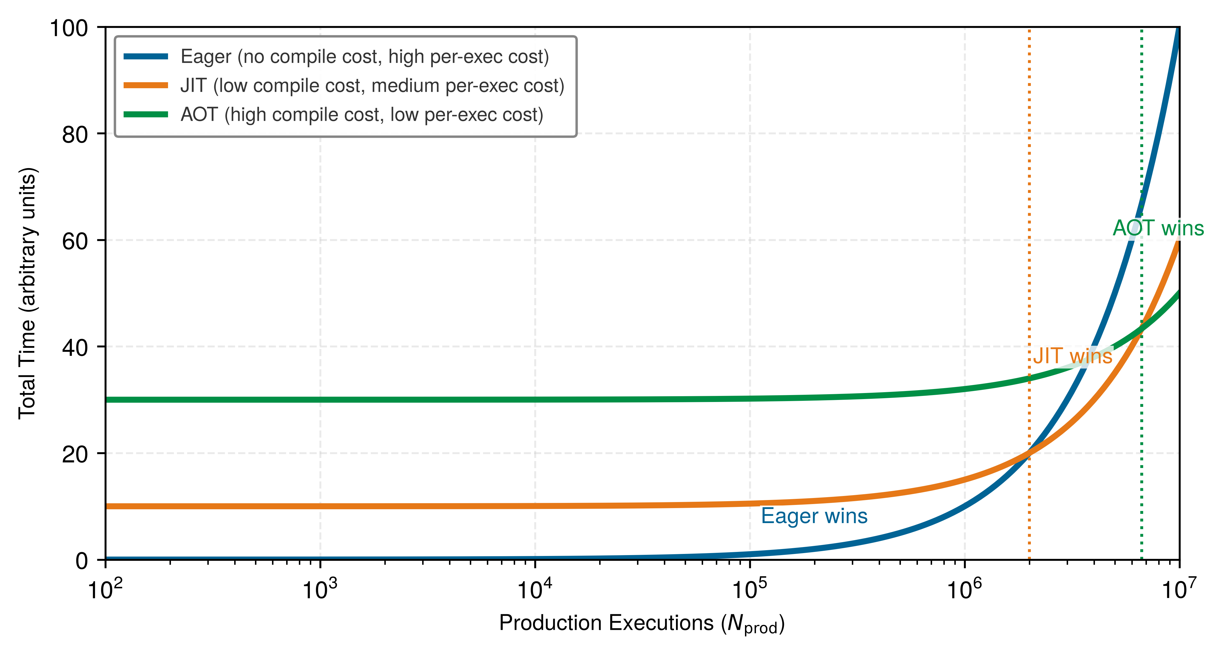
The dispatch overhead law
A second principle, the dispatch overhead law, emerges from equation 4, which identifies the regime in which framework overhead, rather than compute or memory, dominates execution time. Let \(N_{\text{ops}}\) be the number of operations (count), \(t_{\text{dispatch}}\) the per-operation dispatch overhead (seconds), and \(T_{\text{compute}}\) and \(T_{\text{memory}}\) the total compute and memory times (seconds). The ratio uses the additive, no-overlap approximation \(T_{\text{hw}} \approx T_{\text{compute}} + T_{\text{memory}}\); when execution overlaps those costs, measured hardware time should replace their sum. Framework overhead dominates when operations are small relative to dispatch cost:
\[ \text{Overhead Ratio} = \frac{N_{\text{ops}} \cdot t_{\text{dispatch}}}{T_{\text{compute}} + T_{\text{memory}}} \tag{4}\]
When Overhead Ratio \(> 1\), the model is overhead-bound. Compilation can provide its largest gains for overhead-bound workloads because fusion reduces the number of dispatches. The training-step trace in section 1.10 works this effect through end to end, previewed by the numbers that follow.
Summed over \(N_{\text{ops}}\) operations, the per-operation dispatch cost \(t_{\text{dispatch}}\) accumulates into a per-call tax on execution. Whether that tax dominates depends on how the hardware execution time \(T_{\text{hw}}\) compares to the software overhead \(T_{\text{sw}}\) (both measured in seconds), and the regimes split sharply by model size.
The principle’s implication is that workloads composed of small operations can benefit disproportionately from compilation when dispatch dominates execution. Model parameter count alone does not determine the gain.
The dispatch tax analysis reveals that small operations become overhead-bound when dispatch time exceeds device execution time. This observation matters most at the extreme edge of the deployment spectrum, where the Python runtime itself may exceed the target’s resource budget.
Napkin Math 1.2: The dispatch tax
Problem: When does Python overhead kill performance?
Scenario one: Small multilayer perceptron (MLP) (Overhead Bound)
- Compute: 6 ops across small matrix/element-wise operations.
- Hardware time: \(T_{\text{hw}} \approx\) 2.6 μs (mostly memory latency).
- Software overhead: \(T_{\text{sw}} \approx\) 6 ops \(\times\) 15 μs/op = 90 μs.
- Ratio: 90 μs/2.6 μs ≈ 34.6.
- Small-model outcome: The system spends 97 percent of time in host-side dispatch and kernel-launch overhead. Eliminating all modeled dispatch overhead would give an upper-bound speedup of 35.6×.
Scenario two: GPT-3 Layer (Compute Bound)
- Compute: Huge matrix multiplications.
- Hardware time: \(T_{\text{hw}} \approx\) 100 ms = 100000 μs.
- Software overhead: \(T_{\text{sw}} \approx 50 \, \mu s\).
- Ratio: 50 μs/100000 μs ≈ 0.0005.
- Large-model outcome: Modeled Python overhead is negligible. Compilation may still improve fusion, layout, or backend specialization; dispatch elimination contributes little.
Systems insight: Dispatch overhead is regime-dependent. Compilation can reduce host-side overhead for small-operation workloads by fusing operations into fewer launches, while large models benefit mainly from fused kernels and memory movement reductions.
Frameworks for the edge: TinyML and micro-runtimes
The compilation continuum reaches its extreme at the far edge. While cloud frameworks like PyTorch and TensorFlow 2.x prioritize flexibility through eager execution, TinyML16 systems operating on MCUs with kilobytes of memory cannot afford the overhead of a Python interpreter or a fully dynamic runtime.
16 TinyML: Systems designed for MCUs cannot afford a Python interpreter. Micro-runtimes instead use small C/C++ runtimes, fixed memory planning, and model-specific operators. TensorFlow Lite Micro remains interpreter-based: the application supplies a tensor arena whose buffers are planned and reused without heap allocation after setup. Predictable memory is mandatory because exceeding a 256 KB device budget can prevent initialization or inference.
Lighthouse 1.2: Lighthouse example: KWS on TinyML
Scenario: Deploying the Smart Doorbell’s keyword spotting (KWS) model, the DS-CNN Tiny Constraint lighthouse, to an ARM Cortex-M4 with 256 KB RAM and 1 MB Flash.
Constraint: A full PyTorch and Python runtime exceeds the device’s memory budget by orders of magnitude.
Framework solution: Micro-frameworks such as TensorFlow Lite Micro (TFLM) (David et al. 2021) solve this through a tiny interpreter-based runtime with a fixed memory discipline:
- Fixed memory arena: The application supplies a contiguous tensor arena, and the framework plans and reuses buffers from that arena rather than relying on dynamic allocation during inference.
- Kernel selection: Only the specific kernels used by the model (for example, Conv2D, DepthwiseConv) need to be linked or registered with the runtime.
- Compact interpreter execution: The MCU runs a small C/C++ interpreter over a flat model representation, with the model and arena bound at initialization rather than assembled dynamically at runtime.
Silicon contract: On TinyML devices, the contract is strictly memory-bound. The framework’s primary job is to ensure the model’s intermediate activations (the “working set”) fit within the MCU’s tiny SRAM.
David, Robert, Jared Duke, Advait Jain, Vijay Janapa Reddi, Nat Jeffries, Jian Li, Nick Kreeger, et al. 2021. “TensorFlow Lite Micro: Embedded Machine Learning for TinyML Systems.” Proceedings of Machine Learning and Systems 3: 800–811.
These micro-runtimes sacrifice dynamic flexibility to reduce footprint and make memory predictable. With compact models, low-power hardware, and duty cycling, that discipline enables milliwatt-scale inference with mostly on-chip data movement.
The spectrum of execution strategies, from dynamic eager execution to static graph compilation and specialized micro-runtimes, requires developers to make deliberate trade-offs. The key execution-mode decisions summarize these architectural choices:
Checkpoint 1.1: Execution models
The choice of execution mode determines both developer velocity and model performance.
Debuggability vs. speed
Modern compromise
The execution problem determines when computation happens and what optimizations are possible. Neural network training, however, requires a capability that no amount of clever scheduling can provide: the ability to compute gradients automatically.
Consider what training actually requires: for each of millions of parameters, compute how a tiny change would affect the loss. Doing this manually for even a simple three-layer network requires deriving and implementing dozens of partial derivatives. For a modern transformer with billions of parameters, manual differentiation is economically impossible. A framework that executes efficiently but cannot differentiate can run inference but cannot learn.
Self-Check: Question
A GPU performance profile reveals that a sequence of LayerNorm, dropout, and GELU activation operations spends over 80% of its execution time reading and writing intermediate tensors to High Bandwidth Memory (HBM) with very low arithmetic intensity. Why is operator fusion the primary framework optimization for this workload?
- It replaces 16-bit floating-point arithmetic with 8-bit integer arithmetic
- It changes the model architecture to eliminate all non-linear activation functions
- It converts compute-bound matrix multiplications into memory-bound operations
- It fuses multiple sequential element-wise operations into a single GPU kernel, keeping intermediate values in on-chip SRAM/registers and eliminating redundant round trips to HBM
A developer attempts to trace a dynamic PyTorch model containing data-dependent control flow (
if tensor.sum() > 0: ...) using standard graph tracing (torch.jit.trace). What failure mode occurs, and how does modern bytecode graph capture (torch.compile/ TorchDynamo) resolve it?- Standard tracing crashes immediately on any tensor operation, whereas TorchDynamo rewires the Python interpreter into C++
- Standard tracing converts all dynamic control flow into static loops, whereas TorchDynamo disables all GPU acceleration
- Standard tracing records only the branch taken by the example input and silently bakes it into a static graph, whereas TorchDynamo inspects Python bytecode to capture straight-line subgraphs into FX graphs and falls back to the Python interpreter on graph breaks
- Standard tracing successfully compiles dynamic branches using AST inspection, whereas TorchDynamo rejects all conditional statements
State the dispatch overhead law and explain why a workload composed of many small tensor operations on an NVIDIA A100 GPU can be severely underutilized in eager mode even if the GPU has massive compute throughput.
True or False: In
torch.compile, encountering a “graph break” halts program execution and throws a fatal runtime exception because dynamic Python constructs cannot be represented in the computational graph.Order the stages of the
torch.compilecompilation and execution pipeline in PyTorch 2.0, from initial Python function call to hardware execution:AOTAutograd traces both the forward and backward computation graphs ahead of execution
TorchDynamo intercepts Python bytecode during frame evaluation and extracts computational subgraphs
TorchInductor generates optimized vendor-specific kernels (e.g., Triton for GPUs or C++/OpenMP for CPUs)
The high-level intermediate representation is structured as a PyTorch FX graph
The compiled fused kernels execute on the target hardware accelerator
In graph-capture JIT compilation systems like TorchDynamo, an event where the compiler encounters an unsupported dynamic Python construct (such as an unhandled C-extension call or dynamic side effect) and must pause graph capture to yield control to the Python interpreter is called a ____.
Differentiation Problem
The differentiation problem is the task of computing gradients17 automatically. Neural network training requires derivatives of a scalar loss \(\mathcal{L}\) with respect to millions or billions of parameters, making manual differentiation impractical. Because a single scalar loss depends on many parameters, reverse-mode automatic differentiation (AD)18 is normally efficient: one reverse traversal computes all requested parameter gradients, while recovering the same full gradient with forward mode requires one tangent direction per parameter. Major ML frameworks therefore use reverse-mode AD for ordinary scalar-loss training (Baydin et al. 2018).
17 Automatic differentiation (AD): The “automatically” in the triggering sentence is the key word: AD mechanizes the chain rule as a graph traversal, eliminating the manual derivative computation that made scaling beyond toy networks impractical. The systems trade-off that makes this feasible is the choice of reverse mode, which exploits the many-to-one topology of training (many parameters, one scalar loss) to compute all gradients in a single backward pass. Forward mode would require one pass per parameter, making billion-parameter training computationally impossible.
18 Reverse-mode AD: The \(\mathcal{O}(1)\)-vs.-\(\mathcal{O}(P)\) asymmetry of reverse mode has a concrete price: reverse mode retains the operation-dependent values required by derivative rules during the backward traversal. Activation checkpointing changes this saved set by omitting selected values and recomputing them during the backward pass.
Baydin, Atilim Gunes, Barak A. Pearlmutter, Alexey Andreyevich Radul, and Jeffrey Mark Siskind. 2018. “Automatic Differentiation in Machine Learning: A Survey.” Journal of Machine Learning Research 18 (153): 1–43.
Building on the backpropagation algorithm introduced in Neural Computation, the systems engineering of differentiation addresses how frameworks represent computation graphs, manage memory for intermediate values, and orchestrate the backward pass efficiently across accelerators. The framework’s role is not to perform calculus but to manage the bookkeeping at scale, which is required for the training algorithms detailed in Model Training. Listing 7 illustrates the core idea with a simple three-operation function.
def f(x):
    a = x * x  # Square
    b = sin(x)  # Sine
    c = a * b  # Product
    return c
Frameworks decompose this function into elementary operations, each with a known local derivative, and then combine these local derivatives via the chain rule to compute gradients through supported compositions. The systems challenge is implementing this efficiently: the framework must record the computation graph during the forward pass, store intermediate values, and execute the backward pass with minimal memory overhead. Production frameworks solve each of these problems through structured graph recording, intermediate state management, and reverse-mode traversal.
Forward and reverse mode differentiation
Two primary approaches to automatic differentiation exist, and the choice between them (forward mode vs. reverse mode) determines whether gradient computation scales with the number of input or output directions. This distinction explains why neural network training usually relies on reverse mode. Forward mode is useful to understand first because it exposes the bookkeeping directly; reverse mode then appears as the systems response to the many-parameter, one-loss shape of neural network training.
Forward mode
Neural network training usually uses reverse mode (covered next), but forward mode illuminates why reverse mode is efficient for a scalar loss with many parameters. Forward mode automatic differentiation computes directional derivatives alongside the original computation, tracking how changes propagate from input to output. This approach mirrors manual derivative computation, making it intuitive to understand and implement.
Forward mode propagates a tangent alongside each primal value and does not need to retain a reverse tape for a later backward traversal. Its memory and operation overhead depend on the computation and on how many tangent directions are propagated. One seeded execution produces a Jacobian-vector product (JVP). Recovering a full gradient with respect to \(P\) independent inputs requires \(P\) tangent directions, which may be evaluated separately or batched but still scales with the input dimension. Reverse mode instead computes a scalar loss gradient in one backward traversal whose cost depends on the operations rather than the parameter count alone. This asymmetry makes reverse mode the standard choice for neural-network training, while forward-mode JVPs remain useful when the number of input directions is small and in higher-order differentiation methods.
To see the mechanism concretely, consider computing both the value and derivative of \(f(x) = x^2 \sin(x)\). Listing 8 shows how forward mode propagates derivative computations alongside every operation, applying the chain rule and product rule at each step:
def f(x):  # Computing both value and derivative
    # Step 1: x -> x²
    a = x * x  # Value: x²
    da = 2 * x  # Derivative: 2x

    # Step 2: x -> sin(x)
    b = sin(x)  # Value: sin(x)
    db = cos(x)  # Derivative: cos(x)

    # Step 3: Combine using product rule
    result = a * b  # Value: x² * sin(x)
    dresult = a * db + b * da  # Derivative: x²*cos(x) + sin(x)*2x

    return result, dresult
Forward mode achieves this systematic derivative computation by augmenting each number with its derivative value, creating what mathematicians call a “dual number”. Listing 9 runs the same function at \(x = 2.0\), so the bookkeeping becomes concrete: each intermediate value carries its derivative alongside it through a single pass.
x, dx = 2.0, 1.0  # seed: track the derivative with respect to x

a = x * x  # value:      4.0
da = 2 * x  # derivative: 4.0
b = sin(x)  # value:      0.9093
db = cos(x)  # derivative: -0.4161
c = a * b  # value:      3.637
dc = a * db + b * da  # derivative: 1.973
That paired execution propagates one seeded tangent direction alongside the primal values. Its overhead depends on the operations and implementation rather than being exactly 2\(\times\). For a scalar loss with \(P\) parameters, recovering the full gradient through forward mode requires \(P\) independent tangent directions, which may be evaluated separately or batched but still scales with the input dimension.
Forward mode is therefore inefficient for the usual training shape of one scalar loss and millions of parameters. It remains useful when the number of seeded input directions is small and in mixed-mode methods for specialized derivatives such as Jacobian-vector and Hessian-vector products. For the usual scalar-loss training objective, reverse mode reverses this scaling: one backward traversal computes the requested gradients for all parameters that influence the loss.
Reverse mode
Modern ML frameworks normally use reverse mode for scalar-loss training because of computational asymmetry. Forward mode propagates derivatives for selected input directions, while one reverse traversal propagates adjoints from the scalar loss to all requested parameters. The advantage grows with the number of parameters, although the actual cost also depends on the graph and derivative rules.
This asymmetry makes reverse mode the standard choice for neural network training, while forward and mixed modes remain useful for other derivative shapes. Reverse mode runs on the same three-operation function \(f(x) = x^2\sin(x)\) from listing 7, where \(x\) reaches the output through two distinct paths: the square and the sine. Algorithm 1 states the general reverse-mode contract before a worked trace makes one concrete input visible.
\begin{algorithm} \caption{Reverse-mode automatic differentiation} \begin{algorithmic} \Require directed acyclic graph with scalar output $y$; nodes $v_1,\dots,v_n$ in topological order; a local derivative rule for each node \Ensure adjoints $\bar{v}_i = \partial y / \partial v_i$ for the requested input or parameter nodes \For{$i = 1$ to $n$} \State compute $v_i$, record dependencies, and save values requested by its derivative rule \Comment{forward pass} \EndFor \State $\bar{v}_i \gets 0$ for all $i$; $\bar{y} \gets 1$ \For{$i = n$ down to $1$} \For{each parent $u$ of $v_i$} \State $\bar{u} \gets \bar{u} + \bar{v}_i \, \partial v_i / \partial u$ \Comment{accumulate via the chain rule} \EndFor \State release stored values once every rule that needs them has run \EndFor \State \Return the adjoints for the requested nodes \end{algorithmic} \end{algorithm}
The structure of algorithm 1 is also its cost. The forward pass records graph dependencies and retains values requested by backward rules until the reverse traversal consumes them. Reverse mode therefore trades activation and graph memory for an efficient gradient of a scalar output. Checkpointing can save fewer values and recompute them later.
For the concrete function in listing 7 with \(x=2.0\), we record \(a=x^2=4.0\), \(b=\sin(x)\approx0.9093\), and \(c=ab\approx3.637\) during the forward pass. Seeding \(\bar{c}=1.0\), the reverse multiplication gives \(\bar{a}=0.9093\) and \(\bar{b}=4.0\); the square path contributes \(0.9093\cdot4.0\approx3.6372\) to \(\bar{x}\), and the sine path adds \(4.0\cos(2.0)\approx-1.6646\). The final derivative is \(\partial c/\partial x=\bar{x}\approx1.973\).
The critical observation is that this single backward pass computed \(\partial c/\partial x\) regardless of how many paths connect \(x\) to \(c\). In a neural network, each weight can affect the loss through thousands of paths across layers, and reverse mode handles them all in one traversal. This is why training a 175B-parameter model like GPT-3 is feasible at all: reverse mode’s \(\mathcal{O}(1)\) backward passes relative to parameter count keep gradient computation tractable.
Translating this mathematical elegance into a working system requires solving a concrete engineering problem: the backward pass needs values computed during the forward pass, so the framework must decide what to store, when to store it, and when to free it. Modern frameworks accomplish this through computational graphs and automatic gradient accumulation.19
19 Gradient accumulation: The framework processes a large logical batch as smaller mini-batches, freeing each mini-batch’s saved activations after backward while accumulating parameter-sized gradients. Processing 4,096 samples in 64-sample mini-batches can reduce the batch-dependent activation peak by up to 64\(\times\) when activation memory scales linearly with batch size; weights, gradients, optimizer state, and other fixed costs do not shrink. The trade-off is more sequential work before each optimizer update.
Listing 10 illustrates this with a two-layer network, showing both the forward computation that stores intermediate values and the backward pass that consumes them to produce gradients for every parameter simultaneously.
def simple_network(x, w1, w2):
    hidden = x * w1  # First layer
    activated = max(0, hidden)  # ReLU activation
    output = activated * w2  # Second layer
    return output


# --- Forward pass stores intermediates ---
x, w1, w2 = 1.0, 2.0, 3.0
hidden = x * w1
activated = max(0, hidden)
output = activated * w2

# --- Backward pass consumes them ---
d_output = 1.0  # Seed gradient
d_w2 = activated  # = 2.0
d_activated = w2  # = 3.0
d_hidden = d_activated * (1 if hidden > 0 else 0)  # ReLU gate: 3.0
d_w1 = x * d_hidden  # = 3.0
d_x = w1 * d_hidden  # = 6.0
Three implementation requirements emerge from this example. First, the framework must track dependencies between operations to determine the correct reverse traversal order. Second, intermediate values (hidden, activated) must persist in memory until the backward pass consumes them. Third, every operation needs both a forward implementation and a corresponding backward rule. These requirements define the engineering surface of any AD system, and the second requirement, memory persistence, turns out to be the dominant cost.
Memory management strategies
A 175B-parameter model in FP16 requires 350 GB just for weights, beyond a single GPU’s memory. Reverse mode AD also saves operation-dependent forward values for backward. In an illustrative 100-layer network with a batch of 64 images, activations alone can add 8–12 GB alongside weights, gradients, and optimizer state. Memory capacity can therefore set the feasibility boundary even when compute is available.
The saved-activation footprint accumulates across layers. Listing 11 shows how each added layer can contribute another activation tensor that must persist until the backward pass reaches it.
def deep_network(x, w1, w2, w3):
    # Forward pass - must store intermediates
    hidden1 = x * w1
    activated1 = max(0, hidden1)  # Store for backward
    hidden2 = activated1 * w2
    activated2 = max(0, hidden2)  # Store for backward
    output = activated2 * w3
    return output
Frameworks attack this memory wall with two primary strategies. The first is activation checkpointing (also called gradient checkpointing): rather than storing every activation, the framework keeps selected boundary values and recomputes the missing intermediates during the backward pass. At this point, the important systems idea is the runtime contract, not the placement policy. The framework treats some activations as durable checkpoints and treats the rest as values that can be regenerated when the backward traversal reaches them; Gradient accumulation and checkpointing mechanics later examines how training systems choose the checkpoints. Listing 12 makes the runtime contract visible: the forward pass keeps only the segment boundaries, and the backward pass re-runs each segment to regenerate the activations it dropped rather than reading them back from memory.
# Standard backward: every forward activation stays resident
h1 = layer1(x)  # kept for backward
h2 = layer2(h1)  # kept for backward
out = layer3(h2)  # kept for backward

# Checkpointed: keep only the boundary h1 and drop h2. The
# backward pass re-runs the wrapped segment to regenerate
# h2 on demand instead of holding it in memory.
h1 = layer1(x)  # boundary: kept
out = checkpoint(
    lambda a: layer3(layer2(a)), h1
)  # h2 recomputed in backward
The second strategy is operation fusion.20 Rather than executing matrix multiplication, bias addition, and ReLU as three separate operations that materialize intermediate results, frameworks can fuse compatible work into a single kernel. This can accelerate memory-bound portions by keeping intermediate values in registers or caches.
20 Operation fusion: When compatible operations execute as separate kernels, intermediate results may be written to HBM and read back by the next kernel. Fusion can keep those values on chip and avoid the corresponding transfers. The realized benefit depends on the operations, shapes, compiler, and hardware.
Chetlur, Sharan, Cliff Woolley, Philippe Vandermersch, Jonathan Cohen, John Tran, Bryan Catanzaro, and Evan Shelhamer. 2014. “cuDNN: Efficient Primitives for Deep Learning.” arXiv Preprint arXiv:1410.0759.
The backward pass itself benefits from hardware-specific optimization. Rather than directly translating the mathematical definition of a convolution gradient into code, frameworks implement specialized backward kernels that exploit memory access patterns and hardware capabilities of modern accelerators (Chetlur et al. 2014). These optimizations, checkpointing, fusion, and specialized kernels, work together to make training practical for architectures that would otherwise exhaust GPU memory in a single forward pass.
Framework implementation of automatic differentiation
Checkpointing, fusion, and specialized kernels address the systems problems of AD. Frameworks usually expose these mechanisms through high-level APIs. A PyTorch training loop—optimizer.zero_grad(), forward pass, loss.backward(), optimizer.step()—appears to be four function calls. Behind each call, however, the framework tracks operations during the forward pass, builds and maintains the computation graph, manages memory for intermediate values, schedules gradient computations, and interfaces with hardware accelerators. The same graph machinery extends to advanced scenarios: nested torch.autograd.grad calls compute second-order derivatives for techniques like natural gradient descent, and mixed-precision contexts (autocast) select reduced-precision kernels for compute-intensive operations while maintaining FP32 for numerical stability.
PyTorch autograd internals
The autograd system is the framework component that solves the differentiation problem described in section 1.1. Three systems principles govern its design: the data structure that enables efficient gradient computation, the memory cost of maintaining that data structure, and the control mechanisms that production systems require. Understanding these principles explains why training can consume substantially more memory than weight-only inference for the same model, and why frameworks provide specific mechanisms to manage that cost.
The reverse-linked graph structure
During the forward pass, the autograd system constructs a reverse-linked graph of Function nodes. Each node records the operation performed and stores references to the tensors it needs for gradient computation. This graph is the data structure that makes reverse-mode automatic differentiation possible: regardless of how many parameters a model has, a single backward pass through this graph computes all gradients. For a model with \(P\) parameters, reverse-mode AD requires \(\mathcal{O}(1)\) backward passes (compared to \(\mathcal{O}(P)\) for forward-mode), which is why every major framework implements this approach.
Concretely, every tensor produced by a differentiable operation stores a grad_fn attribute pointing to the Function that created it. Each Function links to its inputs through next_functions, forming a chain from the loss back to the leaf parameters. Listing 13 illustrates this structure for a simple computation:
grad_fn links to the Function that created it, forming a reverse chain from output to leaf parameters that enables \(\mathcal{O}(1)\) backward passes.
import torch

x = torch.tensor([2.0], requires_grad=True)
y = x * 3
z = y.pow(2)


# Traverse the reverse-linked graph
print(z.grad_fn)  # PowBackward0
print(z.grad_fn.next_functions)  # -> MulBackward0
print(
    z.grad_fn.next_functions[0][0].next_functions
)  # -> AccumulateGrad (leaf)
The traversal reveals the chain: PowBackward0 (for z = y**2) links to MulBackward0 (for y = x * 3), which terminates at AccumulateGrad for the leaf tensor x. Leaf tensors are the endpoints of the graph where gradients accumulate into the .grad attribute rather than propagating further. The tuple format (Function, index) tracks which output of a multi-output operation each connection corresponds to.
A reverse-linked autograd structure has a critical systems implication: the entire graph must remain in memory from the time a tensor is created until the backward pass consumes it. The graph itself is lightweight (pointers and metadata), but the tensors it references are not, so memory consumption scales with model depth.
The memory-compute trade-off
Every value saved for the backward pass persists until its derivative rule consumes it. These saved values are one major reason training uses more memory than inference, alongside gradients and optimizer state. Different operations save different inputs or outputs, and checkpointing can replace some storage with recomputation.
The illustrative training peak dwarfs weight storage alone.
Consider a sample ResNet-50 training scenario with 25.6M parameters (~102.4 MB of FP32 weights), batch size 64, and \(224{\times}224\) images. With 8 GB–12 GB of saved activations, gradients add ~102.4 MB, and two Adaptive Moment Estimation (Adam) FP32 moment buffers add ~204.8 MB. Summing those four components gives an 8.4 GB–12.4 GB training scenario, roughly 82.1–121.2× the FP32 weight storage alone. It is not a comparison with complete inference memory, which also includes activations and runtime workspaces.
The example shows why training capacity cannot be estimated from weights alone. Both depend on the operations, implementation, and memory reuse, as derived in The true cost of training memory for the four-component training-state equation (\(M_{\text{total}} = M_{\text{weights}} + M_{\text{gradients}} + M_{\text{optimizer}} + M_{\text{activations}}\)) and additional runtime memory.
Frameworks provide three primary mechanisms to manage this trade-off at the graph level. Gradient checkpointing (Chen et al. 2016) changes what the graph preserves: instead of saving all activations, the framework saves selected boundary values and rebuilds the missing intermediates during the backward pass. In iron law terms, checkpointing increases the \(O\) term (recomputation) to reduce the \(D_{\text{vol}}\) term (memory traffic). Tensor detachment provides a complementary mechanism: calling .detach() on a tensor changes which graph edges participate in differentiation, preventing the framework from saving activations through that path. This is essential for transfer learning, where pretrained layers should not accumulate gradients, and it reduces the \(D_{\text{vol}}\) term by eliminating unnecessary activation storage. Mixed-precision training offers a third approach: store selected activations and matrix operations in lower-precision formats so the framework reduces data movement while preserving numerically sensitive work in FP32. Model Training develops these graph mechanisms into sizing decisions.
Chen, Tianqi, Bing Xu, Chiyuan Zhang, and Carlos Guestrin. 2016. “Training Deep Nets with Sublinear Memory Cost.” arXiv Preprint arXiv:1604.06174.
Extensibility and control
Production training systems require fine-grained control over gradient flow that goes beyond the default backward pass. Three categories of control arise in practice. First, selective gradient computation: transfer learning and fine-tuning require freezing subsets of parameters, which the framework supports through requires_grad=False flags and the .detach() mechanism described earlier. Second, gradient inspection and modification: debugging vanishing or exploding gradients, implementing per-tensor gradient clipping, and logging gradient statistics all require intercepting gradients mid-computation, which frameworks expose through hook APIs. Third, custom differentiation rules: operations not in the framework’s built-in library (custom CUDA kernels, novel activation functions, domain-specific operations) require user-defined forward and backward implementations.
These control mechanisms share a common systems design: they are callback-based extensions that the autograd engine invokes at specific points during graph traversal, without modifying the core differentiation algorithm. This extensibility pattern allows the framework to maintain a single optimized backward pass while supporting arbitrarily complex gradient manipulation. In practice, this control appears through a few recurring PyTorch mechanisms: retained graphs, accumulated gradients, custom backward rules, hooks, and safe detachment. Table 6 maps each mechanism to what it controls and what it costs.
| Mechanism | What it controls | Cost or hazard |
|---|---|---|
retain_graph=True |
Keeps saved graph state available for another backward traversal | Retains memory that would otherwise be released; the amount depends on the graph and saved values |
| Gradient accumulation | Successive backward passes sum into .grad until zero_grad() resets them, enabling large effective batches |
Forgetting the reset silently mixes gradients across optimization steps |
Custom autograd.Function |
User-defined forward and backward rules for operations outside the built-in library | Moves the differentiation contract (what to save, how to differentiate) to the implementer |
| Gradient hooks | Inspecting or modifying gradients mid-traversal (clipping, logging, debugging) | Runs arbitrary Python per registered tensor on every backward pass |
.detach() |
Cuts gradient flow at a chosen boundary (frozen layers, inference outputs) | The legacy .data attribute bypasses autograd and silently corrupts gradients; clone before in-place mutation |
One mechanism deserves a closer look because it exposes the differentiation contract most directly. Custom autograd functions move part of that contract from the framework to the implementer: the developer explicitly specifies what to save for the backward pass and how to compute gradients. Listing 14 shows the pattern.
class MultiplyAdd(torch.autograd.Function):
    @staticmethod
    def forward(ctx, x, y, z):
        # Save tensors needed for backward
        ctx.save_for_backward(x, y)
        return x * y + z

    @staticmethod
    def backward(ctx, grad_output):
        # Retrieve saved tensors
        x, y = ctx.saved_tensors

        # Compute gradients using chain rule
        grad_x = grad_output * y  # dL/dx = dL/dout * dout/dx
        grad_y = grad_output * x  # dL/dy = dL/dout * dout/dy
        grad_z = grad_output  # dL/dz = dL/dout * 1

        return grad_x, grad_y, grad_z


# Usage
x = torch.tensor([2.0], requires_grad=True)
y = torch.tensor([3.0], requires_grad=True)
z = torch.tensor([1.0], requires_grad=True)

output = MultiplyAdd.apply(x, y, z)
output.backward()

print(
    x.grad, y.grad, z.grad
)  # tensor([3.]), tensor([2.]), tensor([1.])
These three principles connect directly to the framework’s role as a compiler for the silicon contract. The reverse-linked graph determines which operations the backward pass must execute (the \(O\) term). The memory-compute trade-off governs how much data the framework must move through the memory hierarchy (the \(D_{\text{vol}}\) term). The extensibility mechanisms, in turn, allow engineers to tune both terms for their specific workload. The interaction between autograd memory management and numerical precision leads naturally to mixed-precision training, which further reduces the \(D_{\text{vol}}\) term.
Mixed-precision training support
Mixed precision exploits a hardware asymmetry to improve two iron law terms simultaneously: Tensor Cores execute FP16 matrix multiplications at higher throughput than FP32 CUDA cores (raising \(R_{\text{peak}}\) and reducing the compute term \(O/(R_{\text{peak}} \cdot \eta_{\text{hw}})\)), while FP16 activations halve the memory footprint (reducing \(D_{\text{vol}}\)). Improving both terms simultaneously is rare; most optimizations improve one at the expense of the other.
Automatic mixed-precision APIs use reduced precision for eligible compute-intensive operations and higher precision where backend policy requires it. Matrix multiplications and convolutions commonly use FP16 on supported GPUs, while sensitive operations may use FP32; exact choices depend on the operation, device, and framework. This can preserve model quality and improve speed on suitable hardware. Because FP16 has a narrower dynamic range than FP32, gradients can underflow during backpropagation. Loss scaling addresses this by multiplying the loss before the backward pass, then dividing gradients by the same factor afterward.
Frameworks also support multiple precision modes including FP16, BF16,21 and TF32, NVIDIA’s Tensor Core compute mode for FP32 matrix operations that keeps the FP32 exponent range while using lower mantissa precision. Each mode makes a different trade-off between range and precision. BF16 maintains FP32’s dynamic range, simplifying training by eliminating most gradient underflow issues and often removing the need for loss scaling. Mixed-precision training examines the mechanics of mixed-precision training in detail, including loss scaling algorithms, memory savings analysis, and numerical stability considerations. Listing 15 demonstrates PyTorch’s mixed precision API: the autocast context manager automatically selects FP16 for compute-intensive operations while GradScaler prevents gradient underflow by dynamically scaling loss values.
21 BF16 design rationale: Developed by Google Brain circa 2018 specifically for TPU training stability, BF16 preserves FP32’s eight-bit exponent range while halving memory footprint—an explicit trade-off of mantissa precision (7 bits vs. FP16’s 10) for dynamic range. FP16’s smallest positive normal value is approximately \(6.10 \times 10^{-5}\), but subnormal values extend to approximately \(5.96 \times 10^{-8}\); loss scaling is especially important on hardware or in modes that flush those subnormals to zero. BF16’s FP32-matched exponent largely avoids this class of gradient underflow, eliminating the need for loss scaling in most workloads, which is why BF16 and FP16 are not interchangeable: BF16 is preferred when training stability matters; FP16 is preferred when numerical precision matters more than gradient stability.
import torch
from torch.amp import autocast, GradScaler

model = MyModel().cuda()
optimizer = torch.optim.Adam(model.parameters())
scaler = GradScaler("cuda")

for inputs, targets in dataloader:
    inputs, targets = inputs.cuda(), targets.cuda()
    optimizer.zero_grad()

    # Framework automatically selects precision per operation
    with autocast(device_type="cuda", dtype=torch.float16):
        outputs = model(inputs)
        loss = criterion(outputs, targets)

    # GradScaler handles gradient scaling for numerical stability
    scaler.scale(loss).backward()
    scaler.step(optimizer)
    scaler.update()
BF16 training typically does not require loss scaling. Comparing listing 16 with listing 15 line for line, the GradScaler construction and its scale, step, and update calls all disappear: BF16’s FP32-matched exponent range reduces the gradient-underflow risk that often forces loss scaling, so the loop collapses back to an ordinary backward pass.
# BF16 training typically does not require loss scaling
with torch.autocast(device_type="cuda", dtype=torch.bfloat16):
    outputs = model(inputs)
    loss = criterion(outputs, targets)
loss.backward()  # No GradScaler needed
optimizer.step()
Optimizer state and checkpointing
Resuming training after interruption requires restoring model weights and optimizer state together: momentum buffers, adaptive learning rates, and gradient statistics. For Adam, optimizer state adds about 4\(\times\) the FP16 weight memory (two FP32 states per parameter), so weights plus optimizer state require about 5\(\times\) the FP16 weight footprint. A 7-billion-parameter model therefore requires approximately 70 GB total (14 GB weights + 56 GB optimizer state). Checkpoint size therefore bounds recovery speed after failure, connecting fault tolerance directly to the iron law’s \(D_{\text{vol}}\) term.
Model Training covers optimizer memory requirements and optimization strategies for large-scale training, where checkpoint size becomes a binding constraint. Frameworks provide the state_dict() interface to access optimizer state for serialization (listing 17), and resuming training requires loading both model parameters and optimizer state (listing 18).
import torch
import torch.nn as nn
import torch.optim as optim

model = nn.Linear(10, 5)
optimizer = optim.Adam(model.parameters(), lr=0.001)

# After training steps, optimizer accumulates state
loss = model(torch.randn(3, 10)).sum()
loss.backward()
optimizer.step()

# Access state for checkpointing
state = optimizer.state_dict()
# Contains: {'state': {...}, 'param_groups': [{'lr': 0.001, ...}]}
The mathematics of automatic differentiation were established decades before deep learning’s resurgence. What changed was the systems engineering. Before framework automation, implementing gradient computation for a single fully connected layer meant writing separate forward and backward functions, manually tracking intermediate values, and verifying mathematical correctness across dozens of operations. A modern transformer involves hundreds of operations with complex dependencies; manual gradient derivation for attention, layer normalization, and residual connections would require months of careful work per architecture variant.
# Saving checkpoint
checkpoint = {
    "epoch": epoch,
    "model_state_dict": model.state_dict(),
    "optimizer_state_dict": optimizer.state_dict(),
}
torch.save(checkpoint, "checkpoint.pt")

# Resuming training
checkpoint = torch.load("checkpoint.pt")
model.load_state_dict(checkpoint["model_state_dict"])
optimizer.load_state_dict(checkpoint["optimizer_state_dict"])
The breakthrough was turning this manual process into software infrastructure. A single matrix multiplication requires different gradient computations depending on which inputs require gradients, tensor shapes, hardware capabilities, and memory constraints. Autograd systems handle these variations transparently, which is why the rate of architectural innovation accelerated after frameworks matured. The mathematics did not change; software engineering made the mathematics practical to apply at scale.
Memory management in gradient computation
The memory strategies from section 1.4.1.2 (checkpointing, gradient accumulation) exist because reverse-mode differentiation requires preserving computational history. As listing 11 demonstrated, each layer adds an activation tensor that persists until the backward pass consumes it, creating a memory wave that peaks at the start of backpropagation and recedes as gradients are computed. Modern frameworks track the lifetime of each intermediate value automatically, freeing memory as soon as it is no longer needed. Even with precise lifetime tracking, however, a deeper problem remains: the cost of acquiring memory from the GPU in the first place.
The cost of raw GPU memory allocation provides a critical engineering lesson: production systems require memory abstraction. Device allocation can impose substantial overhead and synchronization. Modern frameworks therefore use caching allocators that retain and reuse device blocks rather than requesting memory for every tensor. Pooling reduces allocation calls and can mitigate fragmentation, but it cannot prevent fragmentation under all allocation patterns.
Systems Perspective 1.2: Caching allocator and utilization
Caching allocators primarily reduce allocation overhead and improve block reuse. Two considerations remain:
- Allocation latency: Reusing a cached block avoids repeated device-allocation calls, whose cost and synchronization behavior depend on the allocator and runtime.
- Fragmentation: Size classes and block splitting improve reuse but can leave free capacity in blocks that do not satisfy a request.
An out-of-memory error can reflect live allocations, allocator-reserved blocks, fragmentation, or another process. nvidia-smi reports device-level usage and is not sufficient by itself to diagnose the framework allocator; allocator-specific memory statistics are needed.
Production system integration challenges
A training iteration can run more slowly in production than in an isolated profile because the full step coordinates with the memory allocator, device manager, operation scheduler, data pipeline, and optimizer. The full-system cost includes work that an operator microbenchmark or isolated kernel profile does not measure. Gradient computation launches accelerator kernels and may require allocation, synchronization, or data movement according to the graph and implementation. These interactions can dominate small-operation workloads and remain measurable at scale. The gap between what the programmer writes (a five-line training loop) and what the system executes (allocations, kernel launches, and synchronization points) is the central tension of AD system design.
The severity of this overhead depends on a deeper architectural choice: how the AD system records and replays computation in the first place. A framework that builds a dynamic trace at runtime pays per-operation bookkeeping on every forward pass, and its caching allocator must accommodate allocation patterns that can vary with execution. A framework that captures a stable computation, by contrast, may pre-plan buffers and reuse storage across the forward and backward graphs because it can reason about lifetimes before execution. The gain depends on capture coverage, tensor lifetimes, shapes, and backend support.
Systems Perspective 1.3: Tape-based vs. transform-based autodiff
PyTorch (tape-based): Records operations on a dynamic “tape” during the forward pass. This is flexible and easy to debug but makes it hard for a compiler to see the whole graph at once for global optimization.
JAX (transform-based): Treats automatic differentiation as a high-level function transformation (grad(f)). JAX traces a pure function for abstract input signatures, allowing compatible transformations such as jit(grad(f)) or vmap(grad(f)) to compose before lowering. This exposes a larger transformed program to accelerator compilers without guaranteeing a single kernel or a universal speed advantage.
The AD system tracks dependencies so it can traverse independent graph branches in a valid order and accumulate gradients correctly. Independent host tasks or explicitly managed device streams can expose concurrency, but ordinary PyTorch autograd work on CUDA follows the framework’s stream semantics rather than automatically assigning every independent branch to a separate stream. Actual overlap depends on runtime scheduling, dependencies, and available device resources.
The memory and system integration challenges examined in section 1.4.1.3 (caching allocators, activation storage, and checkpoint overhead) affect all frameworks. Yet how frameworks implement automatic differentiation in the first place varies significantly, with consequences for both optimization potential and developer experience. The distinction between tape-based and transform-based autodiff captures this architectural divergence. JAX22 exemplifies the transform-based approach, where composable function transformations replace imperative tape recording.
22 JAX: JAX exposes grad, jit, and vmap as transformations on functions; they can be composed when their input and output contracts align, but order matters: vectorizing gradients is not generally the same operation as differentiating a vector-valued result. Compilation can produce fused regions, library calls, and multiple kernels rather than one universal kernel. Transformed functions should be pure; Python side effects may occur during tracing but are not represented in the compiled program, while supported callbacks express intentional runtime effects.
How different frameworks implement AD
The execution models covered in section 1.3, namely eager, static graph, and hybrid, directly shape how each framework implements automatic differentiation:
- PyTorch (Paszke et al. 2019) builds its autograd tape dynamically during forward execution, providing immediate debugging at the cost of graph-level optimization. The
grad_fnchain mechanism detailed in section 1.4.2.1 enables flexible control flow but requires storing the complete graph until backward pass completion. - TensorFlow (Abadi et al. 2016) (in its 1.x incarnation) performed symbolic differentiation during graph construction, enabling ahead-of-time optimization. Modern TensorFlow 2.x uses eager execution by default but provides
tf.functionfor graph compilation when performance matters (TensorFlow Developers 2024). - JAX (Frostig et al. 2018) transforms functions rather than tracking operations. The
jax.grad()transformation returns a new function that computes gradients, enabling composition withjax.vmap()for vectorization andjax.jit()for compilation. This approach requires pure functions but enables composable program transformations that chain differentiation, vectorization, and compilation in a single expression.
Paszke, Adam, Sam Gross, Francisco Massa, Adam Lerer, James Bradbury, Gregory Chanan, Trevor Killeen, et al. 2019. “PyTorch: An Imperative Style, High-Performance Deep Learning Library.” Advances in Neural Information Processing Systems (NeurIPS) 32: 8024–35.
Abadi, Martı́n, Paul Barham, Jianmin Chen, Zhifeng Chen, Andy Davis, Jeffrey Dean, Matthieu Devin, et al. 2016. “TensorFlow: A System for Large-Scale Machine Learning.” Proceedings of the 12th USENIX Symposium on Operating Systems Design and Implementation (OSDI), 265–83.
Frostig, Roy, Matthew James Johnson, and Chris Leary. 2018. “Compiling Machine Learning Programs via High-Level Tracing.” Systems for Machine Learning.
Autodiff implementation differences determine how much debugging visibility, compiler optimization, and deployment portability a team can expect from each framework. A recurring tension runs through every AD design decision: mathematical correctness demands storing computational history, but hardware imposes strict memory limits. Every framework resolves this tension differently, choosing which activations to checkpoint, which operations to fuse, and how aggressively to trade recomputation for memory. These choices determine which models can train on which hardware, making AD system design one of the most consequential engineering decisions in any framework.
Checkpoint 1.2: The systems cost of gradients
Training is inherently more expensive than inference because of Automatic Differentiation.
Computational reality
Optimization mechanics
The execution and differentiation problems together enable the training loop: the execution model determines when computation happens, while automatic differentiation computes the gradients that drive learning. Both problems, however, quietly assume something that cannot be taken for granted: that the same code can run across diverse hardware. A model trained on an NVIDIA A100 must serve inference on a mobile phone’s ARM CPU, a Google TPU, or a microcontroller with kilobytes of memory. The same torch.matmul call must dispatch to cuBLAS on one device and a hand-tuned ARM NEON kernel on another. This hardware diversity creates the third problem.
Self-Check: Question
For a neural network with \(N = 10^7\) parameters and a single scalar loss output \(M = 1\), why do deep learning frameworks uniformly employ reverse-mode automatic differentiation (backpropagation) instead of forward-mode differentiation?
- Reverse-mode computes all \(10^7\) parameter gradients in a single backward pass of complexity \(\mathcal{O}(M) = \mathcal{O}(1)\), whereas forward-mode would require \(10^7\) separate passes of complexity \(\mathcal{O}(N)\)
- Forward-mode differentiation cannot compute exact gradients and relies on finite-difference approximations
- Reverse-mode differentiation requires zero memory allocation for intermediate forward activations
- Forward-mode is restricted exclusively to non-linear activation functions and cannot differentiate matrix multiplications
A PyTorch user modifies an intermediate activation tensor using an in-place operation (
x.relu_()orx += 1) during the forward pass. Duringloss.backward(), autograd raises a runtime error: “one of the variables needed for gradient computation has been modified by an inplace operation”. What is the systems mechanism causing this failure?- In-place operations convert 32-bit floating point numbers to integers, corrupting floating-point precision
- The autograd tape recorded a reference to the forward tensor whose underlying storage was overwritten, destroying the original activation values required by the operation’s derivative formula
- In-place operations automatically set
requires_grad=Falseon all ancestor nodes in the computational graph - The GPU caching allocator prohibits in-place memory modifications during forward execution
Explain the difference between accumulating gradients in a tensor’s
.gradattribute across batches and retaining the autograd computational graph usingloss.backward(retain_graph=True).True or False: Because reverse-mode automatic differentiation computes exact gradients in a single backward pass, its peak memory consumption during training is identical to that of inference.
Order the sequence of events executed during reverse-mode automatic differentiation for a single training step:
Initialize the backward pass by seeding the output gradient adjoint with \(d\mathcal{L}/d\mathcal{L} = 1.0\)
Execute the forward pass while registering operations and saving required activation tensors on the autograd tape
Accumulate calculated parameter gradients into the
.gradattributes of leaf parametersCompute the scalar loss \(\mathcal{L}\) from model outputs and ground truth targets
Traverse the
GradFnDAG backward, applying operation-specific Vector-Jacobian Products (chain rule)To resolve GPU memory exhaustion caused by caching activations during long forward passes, the memory optimization technique that discards intermediate activations and recomputes them on-the-fly from saved boundary tensors during the backward pass is called activation ____ (or rematerialization).
Abstraction Problem
This hardware diversity is architecturally fundamental. GPUs expose abundant throughput-oriented parallelism but have different memory and execution semantics from CPUs. TPUs favor regular tensor programs and compiler-visible shapes. A microcontroller has kilobytes where a server has gigabytes. The abstraction problem therefore requires frameworks to hide this complexity behind a single programming interface while still enabling efficient utilization of each target’s unique capabilities.
The problem decomposes into two interacting dimensions. The first is data representation: how frameworks encode tensors, parameters, and computational state in forms that work across hardware. The second is execution mapping: how high-level operations translate into hardware-specific implementations. These dimensions are not independent concerns. The way data is represented (memory layout, precision, device placement) directly affects what execution strategies are possible. A tensor stored in row-major format on a GPU requires different kernels than one in column-major format on a CPU. A model quantized to INT8 enables entirely different execution paths than FP32.
Solving the abstraction problem requires sophisticated software infrastructure: tensor representations that encode both mathematical semantics and hardware constraints, intermediate representations that enable hardware-specific compilation, and runtime systems that manage data movement across the memory hierarchy. To make this concrete, trace what must happen when a programmer writes model(input). The framework must resolve five decisions in rapid succession: data representation (tensor shape, memory layout, numeric precision), device placement (the bandwidth hierarchy connecting CPU, GPU, and accelerator memory), input delivery (data pipelines that sustain hundreds of MB/s to keep the accelerator fed), model organization (parameters, buffers, and submodules that must move together), and kernel execution (dispatch, scheduling, and resource optimization). These decisions build from the data container up to the hardware execution layer. Distributed placement previews the same abstraction boundary: frameworks expose placement scopes so system components can manage device boundaries, while Model Training analyzes the scaling algorithms and communication costs that make those scopes efficient.
Data structures and tensor abstractions
A ResNet-50 forward pass touches 25.6M parameters, produces intermediate activations at every layer, and must coordinate memory across CPU and GPU address spaces. Frameworks organize all of this data so that a single model(input) call executes millions of operations without the programmer managing a single pointer, by solving four problems in sequence: defining a universal data container (tensors), placing it on the right device (memory management), feeding data fast enough (data pipelines), and dispatching the right hardware kernel (core operations). The path runs from data representation to hardware execution.
Computational graphs specify the logical flow of operations, but data structures determine how those operations access and manipulate data in physical memory. This distinction matters because the same mathematical operation can differ by an order of magnitude in throughput depending on whether data is contiguous in cache, pinned for direct memory access (DMA) transfer, or scattered across pages.
The first step is the data container itself. Framework data structures must sustain memory bandwidth (hundreds of GB/s on modern GPUs), accommodate architectures from 1D sequences to 5D video tensors, and hide device management behind clean APIs. Tensors are the universal answer.
Tensors
At the foundation of every framework’s data representation lies a single abstraction: the tensor, an n-dimensional array that pairs numerical values with the information needed to interpret and place them.
Every computation in a neural network operates on tensors.23 Training batches, activation maps, parameter gradients, and optimizer states are all tensors. This unified representation lets frameworks optimize a single data structure for hardware rather than managing separate containers for each role.
23 Tensor: In mathematics, tensors obey coordinate-transformation laws; ML frameworks use the term more broadly for multidimensional arrays carrying shape, dtype, strides, device placement, and often automatic-differentiation metadata. A transpose commonly creates a strided view, while reshape may return either a view or a copy depending on the layout. These storage semantics make layout relevant to kernel selection and data movement.
Definition 1.2: Tensor
Tensors are \(n\)-dimensional arrays with shape, data type, stride, and device metadata. Framework runtimes use this information to select compatible operations and hardware kernels.
- Significance: A contiguous FP32 tensor of shape \([1024, 1024]\) occupies \(1024{\times}1024{\times}4 = 4{,}194{,}304\) bytes (about 4.2 MB). A noncontiguous view may be accepted directly by a strided kernel or may require materialization when an operation demands a supported contiguous layout.
- Distinction: NumPy arrays also carry shape, dtype, and stride metadata. Framework tensors additionally integrate device placement, automatic differentiation, and accelerator dispatch.
- Common pitfall: Tensor operations may return a new allocation, a view sharing existing storage, or an in-place update, depending on the operation and API variant. Memory accounting must distinguish these cases.
The tensor abstraction consumes far more memory than model weights alone suggest. Engineers who estimate memory from parameter count alone allocate accordingly and encounter out-of-memory errors that seem inexplicable. A quick memory accounting makes the hidden cost concrete: gradients, optimizer momentum, and stored activations accompany every weight tensor.
Napkin Math 1.3: The administrative tax
The illustrative ResNet-50 breakdown in section 1.4.2.1 was ~82.1–121.2× larger than FP32 weight storage alone. The following scenario expands the accounting to gradients, optimizer state, and saved activations at billion-parameter scale.
Problem: How much memory does training state add beyond FP16 weights in this billion-parameter scenario?
Math:
- Model weights: 2 GB.
- Gradients: 2 GB (same size as weights).
- Optimizer states (Adam): 8 GB (\(4 \times\) FP16 weight memory for momentum and velocity stored in FP32).
- Activations: For a batch size of 32 and a 100-layer network, reverse-mode AD retains the operation-dependent values required by derivative rules; activation checkpointing can omit selected values and recompute them during the backward pass. \[ \text{Activations} \approx B \times N_L \times S \times d_{\text{model}} \times n_{\text{saved}} \times 2 \text{ bytes} \] For a 1024-token sequence, 1024-wide hidden state, and 1 saved tensor per layer: \(32 \times 100 \times 1024 \times 1024 \times 1 \times 2 \approx \mathbf{6.7 GB}\). Materialized attention terms can add a separate \(B \times N_{\text{heads}} \times S^2\) component, which is why memory-efficient attention kernels matter.
Systems insight: A 2 GB model carries persistent training state before the first batch is processed (2 GB gradients + 8 GB optimizer state). During a training step, batch-dependent activations add another 6.7 GB, raising the peak “administrative tax” to ~16.7 GB beyond the weights. During training, data movement includes saving and retrieving these activations.
Tensor structure and dimensions
Tensors structure numerical data by adding organizational axes to linear memory layouts. Trace the rank expansion from left to right in figure 8, observing how rank 0 scalars evolve into rank 3 volume tensors.
\scalebox{0.9}{%
\begin{tikzpicture}[font=\small\sffamily]
\begin{scope}
\pgfmathsetmacro{\cubex}{2.5}
\pgfmathsetmacro{\cubey}{2.5}
\pgfmathsetmacro{\cubez}{2.5}
\draw[BrownLine,fill=BrownL!40] (0,0,0) -- ++(-\cubex,0,0) -- ++(0,-\cubey,0) -- ++(\cubex,0,0) -- cycle;
\draw[BrownLine,fill=BrownL] (0,0,0) -- ++(0,0,-\cubez)coordinate(G) -- ++(0,-\cubey,0) -- ++(0,0,\cubez) -- cycle;
\draw[BrownLine,fill=BrownL!70] (0,0,0) -- ++(-\cubex,0,0) -- ++(0,0,-\cubez) -- ++(\cubex,0,0) -- cycle;
\path[red] (-\cubex,-\cubey,0)coordinate(A) -- (0,-\cubey,0)coordinate(B);
\node[below=0.3of $(A)!0.5!(B)$]{Rank 3};
\end{scope}

\begin{scope}[shift={(-5.5,-0.77)}]
\node[draw=BrownLine,fill=BrownL!40,rectangle,%anchor=north west,
minimum width=98,minimum height=98](R){};
\node[right=2pt of $(R.north west)!0.1!(R.south west)$]{1 \ldots ~2};
\node[right=2pt of $(R.north west)!0.24!(R.south west)$]{3 \ldots  ~5};
\node[right=2pt of $(R.north west)!0.39!(R.south west)$]{5 \ldots ~3};
\node[right=2pt of $(R.north west)!0.58!(R.south west)$]{$\vdots$ \phantom{\ldots~} $\vdots$};
\node[right=2pt of $(R.north west)!0.9!(R.south west)$]{3 \ldots ~3};
\node[below=0.3of $(R.south west)!0.5!(R.south east)$]{Rank 2};
\end{scope}

\begin{scope}[shift={(-8.75,-0.77)}]
\node[draw=BrownLine,fill=BrownL!40,rectangle,%anchor=north west,
minimum width=18,minimum height=98](R){};
\node[right=2pt of $(R.north west)!0.1!(R.south west)$]{1};
\node[right=2pt of $(R.north west)!0.24!(R.south west)$]{3};
\node[right=2pt of $(R.north west)!0.39!(R.south west)$]{5};
\node[right=2pt of $(R.north west)!0.58!(R.south west)$]{$\vdots$};
\node[right=2pt of $(R.north west)!0.9!(R.south west)$]{3};
\node[below=0.3of $(R.south west)!0.5!(R.south east)$](R1){Rank 1};
\end{scope}

\begin{scope}[shift={(-10.5,-0.77)}]
\node[draw=BrownLine,fill=BrownL!40,rectangle,%anchor=north west,
minimum width=18,minimum height=18](3R){0};
\end{scope}
\path[red](R1)-|coordinate(P)(3R);
\node[]at(P){Rank 0};
\end{tikzpicture}}In vision applications, raw image inputs map directly onto multi-dimensional tensor layouts. Examine the rank 3 tensor structure in figure 9, observing how red, green, and blue color channels stack along the channel dimension.
Framework tensors carry more than raw numbers. Each tensor stores tensor metadata, runtime information used to validate operations and select fast execution paths: a shape tuple (for example, [64, 3, 224, 224] for a batch of images), a dtype (framework literals such as float32, float16, or int8), and a device tag (CPU, cuda:0). A matrix multiplication, for instance, checks shape compatibility at dispatch time and uses the dtype to route to the correct hardware kernel, whether a standard FP32 GEMM or a Tensor Core FP16 path.
\scalebox{0.75}{%
\begin{tikzpicture}[font=\sffamily\Large]
%
\tikzset{
    Line/.style={line width=1.0pt,black!70,font=\sffamily\footnotesize
},
  Box/.style={align=flush center,
    inner xsep=4pt,
    node distance=0,
    draw=white,
    line width=0.75pt,
    fill=red!80,
    minimum width=10mm,
    minimum height=10mm
  },
}
\node[Box](B1){\textbf{6}};
\node[Box,right=of B1](B2){\textbf{2}};
\node[Box,right=of B2](B3){\textbf{5}};
\node[Box,below=of B1](B4){\textbf{32}};
\node[Box,right=of B4](B5){\textbf{15}};
\node[Box,right=of B5](B6){\textbf{4}};
\node[Box,below=of B4](B7){\textbf{1}};
\node[Box,right=of B7](B8){\textbf{8}};
\node[Box,right=of B8](B9){\textbf{3}};
%%
\node[Box,fill= OliveLine, draw= white,above=of B2](2B1){\textbf{8}};
\node[Box,fill= OliveLine, draw= white,right=of 2B1](2B2){\textbf{7}};
\node[Box,fill= OliveLine, draw= white,right=of 2B2](2B3){\textbf{5}};
\node[Box,fill= OliveLine, draw= white,below=of 2B3](2B4){\textbf{1}};
\node[Box,fill= OliveLine, draw= white,below=of 2B4](2B5){\textbf{2}};
%%
\node[Box,fill= BlueLine!80, draw= white,above=of 2B2](3B1){\textbf{2}};
\node[Box,fill= BlueLine!80, draw= white,right=of 3B1](3B2){\textbf{1}};
\node[Box,fill= BlueLine!80, draw= white,right=of 3B2](3B3){\textbf{9}};
\node[Box,fill= BlueLine!80, draw= white,below=of 3B3](3B4){\textbf{4}};
\node[Box,fill= BlueLine!80, draw= white,below=of 3B4](3B5){\textbf{3}};
%
\draw[dashed,Line,latex-latex]([yshift=-3mm]B7.south west)--
            node[below=1mm]{Width: 3 Pixels}([yshift=-3mm]B9.south east);
\draw[dashed,Line,latex-latex]([xshift=-4mm]B7.south west)--
            node[left]{Height: 3 Pixels}([xshift=-4mm]B1.north west);
\draw[dashed,Line,latex-latex,shorten <=2mm]([xshift=-4mm]B1.north west)--
            node[left=3mm,pos=0.6]{3 Color Channels}([xshift=-4mm]3B1.north west);
\end{tikzpicture}}Memory layout implementation introduces distinct challenges in tensor design. While tensors provide an abstraction of multi-dimensional data, physical computer memory remains linear. Stride patterns address this disparity by creating mappings between multi-dimensional tensor indices and linear memory addresses. These patterns significantly impact computational performance by determining memory access patterns during tensor operations. Figure 10 makes this concrete with a \(2{\times}3\) tensor: follow the same six values as they map into two different linear orderings—row-major and column-major—and note how the stride values change to compensate.
\begin{tikzpicture}[font=\footnotesize\sffamily]
% Define colors
\definecolor{col1}{RGB}{135, 206, 250}
\definecolor{col2}{RGB}{255, 182, 193}
\definecolor{col3}{RGB}{152, 251, 152}
% 2x3 tensor visualization (LEFT SIDE)
\foreach \row in {0,1} {
  \foreach \col in {0,1,2} {
    \pgfmathsetmacro{\val}{\row * 3 + \col + 1}
    \node[draw, minimum width=15mm, minimum height=10mm,
          fill=col1!50](B\row\col) at (\col*1.7, 1-\row*1.2) {\val};
  }
}
\node[above=2pt of B01]{\textbf{2D Tensor ($2{\times}3$)}};
\path[red](B02.north east)--++(3.5,0)coordinate(CR);
\path[red](B12.340)--++(3.5,0)coordinate(ZE);
% Row-major memory layout (RIGHT SIDE)
\foreach \i in {0,1,2,3,4,5} {
  \pgfmathsetmacro{\val}{\i + 1}
  \node[draw, minimum width=11mm, minimum height=8mm,
        anchor=north west,fill=col2!50](CB\i) at ($(CR)+(\i*1.1, 0)$) {\val};
  \node[below=0pt of CB\i, font=\tiny\sffamily]  {[\i]};
}
\node[above=2pt of CB2.north east]{\textbf{Row-Major Layout}};
% Column-major memory layout (RIGHT SIDE)
\foreach \i in {0,1,2,3,4,5} {
  \pgfmathtruncatemacro{\val}{mod(\i,2)*3 + int(\i/2) + 1}
  \node[draw, minimum width=11mm, minimum height=8mm,
         anchor=north west,fill=col3!50](ZE\i) at ($(ZE)+(\i*1.1, 0)$) {\val};
  \node[below=0pt of ZE\i, font=\tiny\sffamily] {[\i]};
}
\node[above=2pt of ZE2.north east]{\textbf{Column-Major Layout}};
% Strides explanation (BOTTOM)
\node[anchor=north west,align=left,inner sep=0pt,font=\fontsize{9pt}{12}\selectfont\sffamily]
at ($(B10.south west)+(0,-0.3)$) {%
\textbf{Stride Calculation:}\\
Row-major strides: [3, 1]\\
Column-major strides: [1, 2]\\
Element [i,j] offset = i$\times$ stride[0] + j$\times$ stride[1]
};
\end{tikzpicture}Stride choices become performance choices. Row-major layout (used by NumPy, PyTorch) stores elements row by row, making row-wise operations more cache-friendly. Column-major layout (used by some BLAS libraries) stores elements column by column, optimizing column-wise access patterns. The stride values encode this layout information: in row-major layout for a \(2{\times}3\) tensor, moving to the next row requires skipping three elements (stride[0] = 3), while moving to the next column requires skipping one element (stride[1] = 1).
These memory layout details have direct performance implications, but no ordering is universally superior. Efficient access depends on which dimension an operation traverses, the kernel’s supported layouts, vectorization, and the target memory hierarchy. A mismatched layout may require strided access or a conversion, while a kernel designed for that layout can access it efficiently.
The dtype is the tensor-level lever that trades numerical range against data movement. The standard choice in machine learning has been FP32 precision, exposed in frameworks through dtype literals such as float32, offering a balance of precision and efficiency. Modern frameworks extend this with multiple numeric types for different needs. Integer types support indexing and embedding operations. Reduced-precision types like FP16 enable efficient mobile deployment. INT8 precision allows fast inference on specialized hardware. The choice of numeric type affects both model behavior and computational efficiency: neural network training typically requires FP32 precision for critical accumulations to maintain stable gradient computations, while inference tasks can often use lower precision (framework dtype literals such as int8 or even int4, corresponding to INT8 and INT4), reducing memory usage and increasing processing speed. Mixed-precision training approaches combine these benefits by using FP32 for critical accumulations while performing most computations at lower precision.
Type conversions become another point where abstraction meets physics. Operating on tensors with different types demands explicit conversion rules to preserve numerical correctness. These conversions introduce computational costs and risk precision loss. Frameworks provide type casting capabilities but rely on developers to maintain numerical precision across operations.
Tensors answer the data-representation problem by encoding shape, layout, and precision into a single abstraction. A perfectly shaped tensor on the wrong device, however, or one that must cross the PCIe-to-HBM bandwidth gap to reach the GPU, can erase every layout optimization. The next problem is placement: where data lives and how it moves.
Device and memory management
Tensors and their memory layouts establish what the framework computes with. Where that data physically resides, and how it moves between locations, determines whether computation happens at full speed or crawls.
Frameworks as the operating system interface
While the high-level API focuses on math, the framework’s backend functions as the operating system of the Single-Machine Stack. It manages the two critical resources of a single node: compute scheduling and data movement.
The CUDA Runtime serves as this OS layer, providing the low-level primitives for launching kernels and managing device memory. The framework coordinates with this runtime to implement DMA over the PCIe bus. The bandwidth gap between the host (CPU) and device (GPU) is the primary “Data Loading Bottleneck”: Bandwidth vs. latency models this transfer, separating the two constraints, \(T = L_{\text{lat}} + D_{\text{vol}}/\text{BW}\), that determine whether a given data-loading strategy is limited by per-transfer latency or by sustained bandwidth. Frameworks mitigate this through pinned memory (page-locked host memory), which enables DMA transfers without pageable-memory staging. This “HW/OS” interface is what makes high-throughput training loops possible on a single machine.
Every tensor resides on a specific device, and cross-device operations incur transfer costs that can dominate execution time. PCIe 4.0 delivers 32 GB/s between CPU and GPU, while HBM2e provides 2.04 TB/s within the GPU. This 63.7× bandwidth gap means a single misplaced tensor transfer can erase the entire speedup from GPU acceleration.
Interconnect bandwidth spans ~64\(\times\): HBM far above NVLink, NVLink far above PCIe.
Device placement matters for framework design because the framework must track where every tensor lives and enforce that operations only combine tensors on the same device. When data must move, the framework must decide whether to block execution or overlap the transfer with other work. These decisions, invisible to most users, can move a training loop from transfer-bound execution toward substantially higher hardware utilization.
Three systems principles govern effective device and memory management: understanding the bandwidth hierarchy that constrains data movement, overlapping computation with communication to hide transfer latency, and using fine-grained synchronization to maintain correctness without sacrificing concurrency, supported by quantitative analysis grounded in the iron law’s data movement term. The bandwidth hierarchy provides the first constraint.
The cost of moving data between devices varies by orders of magnitude depending on the interconnect.24 Table 7 shows transfer times for a \(1000{\times}1000\) float32 tensor (4 MB)—roughly the size of a typical activation tensor in a moderately sized model. The numbers reveal why careless device placement can erase any speedup from GPU acceleration.
24 NVLink: NVIDIA’s high-bandwidth GPU-to-GPU interconnect (see Hardware Acceleration), providing 600 GB/s bidirectional bandwidth (NVLink 3.0 on A100) compared to 64 GB/s for PCIe 4.0 x16. This ~10\(\times\) bandwidth advantage determines whether tensor parallelism, splitting one large tensor computation across multiple GPUs, is practical for a given model size: GPUs connected only by PCIe can make the \(D_{\text{vol}}/\text{BW}\) communication term dominate total training time, erasing the benefit of additional compute.
| Interconnect | Bandwidth | Transfer Time | Path |
|---|---|---|---|
| PCIe 3.0 x16 | 15.8 GB/s | 0.254 ms | Host to device |
| PCIe 4.0 x16 | 32 GB/s | 0.125 ms | Host to device |
| NVLink 3.0 | 300 GB/s per direction (600 GB/s bidirectional) | 0.013 ms | GPU to GPU |
| GPU Memory | 2039 GB/s | 0.002 ms | On device |
These numbers connect directly to the iron law of performance. Every cross-device transfer contributes to \((D_{\text{vol}}/\text{BW})\) at a fraction of on-device bandwidth. Dividing 1 GB by the stated PCIe 4.0 peak gives 31.2 ms, a bandwidth-only lower bound that omits protocol, launch, synchronization, topology, and contention overhead. Transfers can dominate lightweight or small-batch workloads, so deployed latency must be measured rather than inferred from peak bandwidth alone.
Every tensor should reside on the device where it will be consumed, and transfers should occur only when unavoidable. Frameworks track device placement for every tensor and raise errors when operations attempt to combine tensors from different devices, enforcing this discipline at the API level.
Overlapping computation and communication
When transfers are unavoidable, the next optimization is to hide their latency by executing them concurrently with computation. Modern GPUs contain independent hardware units for computation (SM clusters) and data transfer (copy engines), enabling true simultaneous execution. The framework abstraction that exposes this hardware parallelism is the CUDA stream: an independent execution queue where operations execute sequentially within a stream but concurrently across streams.
Without explicit concurrency control, the GPU serializes all operations on a single default stream, leaving execution units idle while data transfers complete. By placing data transfers on one stream and computation on another, the effective latency approaches the theoretical minimum of \(\max(\text{compute\_time}, \text{transfer\_time})\) rather than their sum. Stream-based overlap effectively hides the \(D_{\text{vol}}/\text{BW}\) penalty when computation is the longer operation (see listing 19).

Overlapping copy and compute costs max(copy, compute), not their sum.
The non_blocking=True flag requests an asynchronous copy with respect to the host when the backend supports it. For host-to-device copies, pinned memory is generally required to overlap the transfer with other device work; pageable memory may be staged internally, and the call’s host-blocking behavior is implementation-dependent. Correct overlap also requires compatible hardware, separate execution resources, and explicit dependency management.
The same synchronization pattern appears when model stages overlap across microbatches. Listing 20 shows each stage running on its own stream, with events enforcing only the producer-consumer dependencies needed for correctness.
compute_stream = torch.cuda.Stream()
transfer_stream = torch.cuda.Stream()

# Transfer next batch while computing
# current batch
with torch.cuda.stream(transfer_stream):
    next_batch = next_batch_cpu.to("cuda", non_blocking=True)

with torch.cuda.stream(compute_stream):
    output = model(current_batch)
    loss = criterion(output, labels)

# Pinned host memory can enable transfer overlap
x_pinned = torch.randn(1000, 1000).pin_memory()
x_gpu = x_pinned.to("cuda", non_blocking=True)  # Asynchronous

# A pageable source may require staging and
# should not be assumed to overlap
y_regular = torch.randn(1000, 1000)
y_gpu = y_regular.to("cuda", non_blocking=True)# Pipeline parallelism: place stages on separate GPUs
devices = [torch.device(f"cuda:{i}") for i in range(3)]
stages = [
Stage1().to(devices[0]),
Stage2().to(devices[1]),
Stage3().to(devices[2]),
]
streams = [torch.cuda.Stream(device=device) for device in devices]
events = [
[torch.cuda.Event() for _ in range(num_microbatches)]
for _ in stages
]
outputs = [[None] * num_microbatches for _ in stages]
for mb in range(num_microbatches):
for stage_idx, (stage, stream, device) in enumerate(
zip(stages, streams, devices)
):
with torch.cuda.device(device), torch.cuda.stream(stream):
if stage_idx > 0:
# Wait for previous stage to complete
# this microbatch
events[stage_idx - 1][mb].wait()
stage_input = outputs[stage_idx - 1][mb].to(
device, non_blocking=True
)
else:
stage_input = inputs[mb].to(device, non_blocking=True)
outputs[stage_idx][mb] = stage(stage_input)
events[stage_idx][mb].record()This overlap principle extends naturally to model-stage overlap within a single node. Different model stages on separate GPUs can process different microbatches concurrently, with each stage’s computation overlapping the next stage’s data reception (see listing 20). Model Training later names and analyzes the distributed-training strategies built from this scheduling pattern; here, the single-node implementation is enough to expose the synchronization principle that survives at larger scale. Once computation and communication overlap, the remaining challenge is ensuring correctness when operations complete out of order.
Synchronization and correctness
Concurrent execution introduces ordering constraints. When one stream’s output becomes another stream’s input, the system must enforce a happens-before relationship without unnecessarily serializing independent work. Two synchronization mechanisms exist, with dramatically different performance implications.
Full device synchronization (torch.cuda.synchronize()) blocks all streams and the CPU until every queued operation completes. This creates a global serialization point that eliminates all overlap benefits. CUDA events provide the alternative: fine-grained synchronization that blocks only the dependent stream, allowing other streams and the CPU to continue execution (see listing 21).
# Create streams and event
stream1 = torch.cuda.Stream()
stream2 = torch.cuda.Stream()
event = torch.cuda.Event()

# Stream 1: producer
with torch.cuda.stream(stream1):
    result1 = expensive_computation(data1)
    event.record()  # Mark completion point

# Stream 2: consumer (waits only for stream1's event)
with torch.cuda.stream(stream2):
    event.wait()  # Block stream2 until event is recorded
    result2 = dependent_computation(result1)  # Safe to use result1
The performance difference between these approaches is not incremental but categorical. Full synchronization after every operation converts a concurrent pipeline into a sequential one, entirely negating the hardware parallelism that streams expose. Event-based synchronization preserves the concurrent execution model while enforcing only the dependencies that correctness requires.
Device placement discipline protects the bandwidth hierarchy from accidental PCIe traffic. Every tensor carries a device attribute, and frameworks enforce a strict invariant: operations can only combine tensors on the same device. A RuntimeError results from mixing cuda:0 and cuda:1 tensors, preventing silent cross-device transfers.
The movement mechanism is explicit. Tensor .to() returns the original tensor when its dtype and device already match the request; otherwise it returns a converted copy unless copy=True forces a copy. Module .to() modifies registered parameters and buffers in place and returns the module.
The performance discipline follows from the bandwidth gap: allocate tensors on the target device from the start rather than creating them on CPU and transferring them, reuse GPU memory across iterations rather than reallocating it, and colocate inputs, labels, and model parameters on the same device to eliminate implicit transfers. At 32 GB/s, violating any of these principles inserts PCIe transfers into the critical path that can dominate a training iteration that otherwise runs at 2.04 TB/s on-device.
The same synchronization discipline has one operational trap: debug code often leaves torch.cuda.synchronize() in the hot path, turning an overlapped pipeline into a serialized one. When overlap remains poor, profiling must separate scheduling stalls from kernel inefficiency. NVIDIA Nsight Systems (nsys profile) shows CPU activity, GPU kernels, and memory transfers on one timeline. NVIDIA Nsight Compute (ncu) then explains kernel behavior with hardware counters.
Table 8 is the diagnostic map for that second step. SM means streaming multiprocessor, the GPU block that schedules groups of threads; a warp is one scheduled thread group.
| Metric | Meaning | Optimization Target |
|---|---|---|
| SM Occupancy | Active warps/maximum warps | Increase parallelism if low |
| Memory Throughput | Achieved/peak bandwidth | Optimize memory access patterns |
| Compute Throughput | Achieved/peak FLOP/s | Reduce memory bottlenecks |
| Tensor Core Active | Time in Tensor Core ops | Verify mixed-precision utilization |
Data pipelines and loading

Each DataLoader knob relieves a specific input bottleneck.
Streams and events address placement and movement by overlapping transfers with computation so that the GPU rarely stalls on a single tensor. Scheduling alone, however, cannot help if data arrives too slowly in the first place. The next constraint is input delivery: data must arrive fast enough to sustain throughput. The core systems principle is straightforward: the data pipeline must sustain the accelerator’s consumption rate. A GPU processing 1,000 images per second at 224 by 224 resolution requires approximately 150.5 MB/s of sustained raw uint8 image throughput. If the pipeline cannot maintain this rate, the accelerator idles and the effective utilization term in the iron law drops below 1.
Frameworks address this throughput requirement through three mechanisms. The first is parallel worker processes: the DataLoader spawns multiple CPU processes, each independently loading and preprocessing samples. When storage access, decoding, augmentation, or normalization makes one loader process too slow to feed the accelerator, multiple workers can overlap I/O wait with preprocessing. Once the input pipeline meets demand, extra workers add overhead rather than throughput. When num_workers > 0, the DataLoader distributes sample indices across workers through a shared queue, and workers push completed samples to a data queue that the main process assembles into batches.
The second mechanism is prefetching. With multiprocessing enabled, prefetch_factor controls how many batches each worker prepares in advance. Four workers with prefetch_factor=2 can maintain up to eight prefetched batches, increasing the chance that input work overlaps accelerator computation. Prefetching cannot guarantee that the accelerator never stalls; storage, decoding, augmentation, and contention can still make production slower than consumption. The cost is additional host memory proportional to the queued data.
The third mechanism is pinned memory for DMA transfers. The pin_memory=True option places batches in page-locked host memory, which can avoid pageable-memory staging and enable host-to-device copies to overlap device work. For a batch of 64 FP32 images at \(224{\times}224{\times}3\) (38.5 MB), dividing by the stated PCIe 4.0 x16 peak gives 1.2 ms; this is a bandwidth-only lower bound, not a measured pinned-transfer latency. The realized benefit over pageable memory depends on the platform, batch size, pipeline, and overlap. Pinned pages also reduce pageable system memory.
The DataLoader configuration is useful only when each parameter is tied to a bottleneck. In this configuration, num_workers enables parallel loading, prefetch_factor controls pipeline depth, and pin_memory enables DMA transfers. The worker count is a throughput/memory trade-off, not a universal constant. A practical starting point is setting num_workers equal to the number of available CPU cores, then adjusting based on whether loading is I/O-bound or CPU-bound. For I/O-bound workloads such as reading images from network storage, more workers overlap disk latency and improve throughput. For CPU-bound workloads involving heavy augmentation, the benefit saturates once all cores are in use. Too many workers waste memory, since each maintains a copy of the Dataset object.
Once throughput is high enough, worker process management becomes a correctness constraint. PyTorch assigns each worker a distinct PyTorch seed. A worker_init_fn is still useful when dataset or augmentation code also uses NumPy or Python’s random module, as listing 22 demonstrates. Shared Python state is generally process-local, so modifications in one worker do not automatically propagate to the others or the main process; explicitly shared or memory-mapped storage is needed when workers must share mutable state.
The Dataset choice is another throughput decision because it determines how samples can be scheduled. PyTorch supports two dataset paradigms. Map-style datasets implement __len__ and __getitem__, enabling random access to samples by index—this pattern works well for datasets that fit in memory or support efficient random access on disk. Iterable-style datasets implement __iter__ instead, yielding samples sequentially for streaming data sources where random access is impractical. Map-style datasets support sampler-based shuffling, while iterable datasets must implement any ordering or buffered shuffling within the iterator or data source.
num_workers parallelizes I/O and preprocessing across CPU cores, prefetch_factor controls pipeline depth, and pin_memory enables DMA transfers to the GPU.
import random

import numpy as np
import torch
from torch.utils.data import DataLoader


def seed_worker(worker_id):
    worker_seed = torch.initial_seed() % 2**32
    np.random.seed(worker_seed)
    random.seed(worker_seed)


loader = DataLoader(
    dataset,
    batch_size=64,
    shuffle=True,
    num_workers=4,  # Parallel worker processes (mechanism 1)
    prefetch_factor=2,  # Batches prepared ahead per worker (mechanism 2)
    pin_memory=True,  # Page-locked memory for DMA (mechanism 3)
    worker_init_fn=seed_worker,  # Reproducible augmentation per worker
)

# Pipeline effect: while GPU processes batch N,
# 4 workers load batches N+1..N+8 into pinned memory,
# ready for DMA transfer when the GPU finishes.
Collation is the final place where representation choices affect throughput. The collate_fn parameter determines how individual samples are combined into batches. The default collation stacks tensors along a new batch dimension, which works when all samples have identical shapes. For variable-length data such as text sequences, custom collation handles padding, sorting by length, or creating attention masks—directly affecting both memory usage and training throughput.
DataLoaders, Datasets, and collation functions solve input delivery by sustaining accelerator-rate throughput through parallelism, prefetching, and DMA. These structures, however, handle only ephemeral data: samples flow through the pipeline once per epoch and are discarded. The next framework responsibility is persistent state, especially the model’s own weights when those weights exceed the memory of any single device.
Parameter structures
A GPT-3 scale model stores 175B parameters, occupying 350 GB in FP16. Managing these parameters across devices, keeping gradients synchronized, and maintaining optimizer state (Adam state alone can add about 4\(\times\) the FP16 weight memory, as the Administrative Tax notebook showed) is a core framework responsibility. Because parameters persist throughout training and inference, frameworks organize them into compact structures that minimize memory while enabling fast read and write access. During multi-GPU training, frameworks may replicate parameters across devices for parallel computation while keeping a synchronized master copy; parameter-server systems are one communication-efficient design for workers to read and write globally shared parameters (Li et al. 2014). Synchronizing multi-billion parameter models can require transferring tens of GB of gradients per step, which is why frameworks expose communication backends that can synchronize tensors efficiently. Model Training later names the specific collective operations and scaling strategies.
Li, Mu, David G. Andersen, Jun Woo Park, Alexander J. Smola, Amr Ahmed, Vanja Josifovski, James Long, Eugene J. Shekita, and Bor-Yiing Su. 2014. “Communication Efficient Distributed Machine Learning with the Parameter Server.” Advances in Neural Information Processing Systems (NeurIPS) 27: 19–27.
Parameter structures must also adapt to varying precision requirements. Training typically uses FP32 for gradient stability, but inference and large-scale training increasingly use FP16 or INT8. Frameworks implement type casting and mixed-precision management to enable these optimizations without compromising numerical accuracy.
Distributed execution contexts
The computational graph defines what to compute, but where and how that computation runs across devices is the job of execution contexts. On a single node, execution contexts manage CUDA streams and events (introduced in section 1.5.1.3) to overlap computation and data transfer across GPUs.
When training scales beyond a single machine, these same abstractions extend to named groups of devices. Frameworks use constructs like ProcessGroup (PyTorch) or Mesh (JAX) to describe which tensors and operations belong together, relying on communication libraries like NCCL to execute collective primitives—such as ring-AllReduce for gradient aggregation and AllGather for parameter gathering. The runtime manages these primitives to maximize interconnect utilization: intra-node NVLink links deliver up to \(900\text{ GB/s}\) of bi-directional bandwidth per GPU, whereas inter-node InfiniBand or Ethernet networks drop to \(50\text{--}400\text{ Gbps}\) (\(6.25\text{--}50\text{ GB/s}\)), making collective communication efficiency the primary bottleneck in distributed training scaling. The important framework idea is the abstraction boundary: user code names placement relationships, and the framework preserves those relationships while the hardware path changes underneath.
These concepts appear here because they shape framework API design even before the book asks the reader to reason about distributed-training algorithms. The details of gradient synchronization, communication topologies, and fault tolerance build on these foundations later. For now, the only point needed is placement expressiveness: when models exceed single-device memory, frameworks must give the training system more than one way to place work. A GPT-3 scale model, for instance, cannot fit on a single GPU—its 175B parameters alone require 350 GB in FP16, far exceeding any GPU’s memory. Figure 11 previews the framework placement idea without requiring the full distributed-training machinery yet: a system can split work across layer groups, across replicated batches, or within very large tensors. Scaling Training Systems later formalizes these dimensions as training strategies and analyzes their communication costs.
\resizebox{0.6\textwidth}{!}{
\begin{tikzpicture}[line cap=round,line join=round,font=\small\sffamily]
\tikzset{
pics/square/.style = {
        code = {
        \pgfkeys{/channel/.cd, #1}
\begin{scope}[local bounding box=SQUARE,scale=\scalefac,every node/.append style={transform shape}]
% Right Face
\draw[fill=\channelcolor!70,line width=\Linewidth]
(\Depth,0,0)coordinate(\picname-ZDD)--(\Depth,\Width,0)--(\Depth,\Width,\Height)--(\Depth,0,\Height)--cycle;
% Front Face
\draw[fill=\channelcolor!40,line width=\Linewidth]
(0,0,\Height)coordinate(\picname-DL)--(0,\Width,\Height)coordinate(\picname-GL)--
(\Depth,\Width,\Height)coordinate(\picname-GD)--(\Depth,0,\Height)coordinate(\picname-DD)--(0,0,\Height);
% Top Face
\draw[fill=\channelcolor!20,line width=\Linewidth]
(0,\Width,0)coordinate(\picname-ZGL)--(0,\Width,\Height)coordinate(\picname-ZGL)--
(\Depth,\Width,\Height)--(\Depth,\Width,0)coordinate(\picname-ZGD)--cycle;
\end{scope}
    }
  }
}
\pgfkeys{
  /channel/.cd,
  Depth/.store in=\Depth,
  Height/.store in=\Height,
  Width/.store in=\Width,
  channelcolor/.store in=\channelcolor,
  drawchannelcolor/.store in=\drawchannelcolor,
  scalefac/.store in=\scalefac,
  Linewidth/.store in=\Linewidth,
  picname/.store in=\picname,
  Depth=1.6,
  Height=1.1,
  Width=1.4,
  channelcolor=BrownLine,
  drawchannelcolor=BrownLine,
  scalefac=1,
  Linewidth=1.0pt,
  picname=C
}
\def\ras{0.95}
\def\dis{2.2}
\begin{scope}[local bounding box=BELOW,shift={($(0,0)+(0,0)$)},scale=1,every node/.append style={transform shape}]
\begin{scope}[local bounding box=GPU0,shift={($(0,0)+(0,0)$)},scale=1,every node/.append style={transform shape}]
 \foreach \i in {1,...,4} {
 \pic[shift={(0,0)}] at  ({-\i*\ras}, {-\ras*\i}) {square={scalefac=1,picname=4,channelcolor=BlueLine,Linewidth=0.7pt}};
  }
\end{scope}
\begin{scope}[local bounding box=GPU8,shift={($(0,0)+(\dis,0)$)},scale=1,every node/.append style={transform shape}]
 \foreach \i in {1,...,4} {
 \pic[shift={(0,0)}] at  ({-\i*\ras}, {-\ras*\i}) {square={scalefac=1,picname=12,channelcolor=RedLine,Linewidth=0.7pt}};
  }
\end{scope}
\begin{scope}[local bounding box=GPU16,shift={($(0,0)+(2*\dis,0)$)},scale=1,every node/.append style={transform shape}]
 \foreach \i in {1,...,4} {
 \pic[shift={(0,0)}] at  ({-\i*\ras}, {-\ras*\i}) {square={scalefac=1,picname=20,channelcolor=GreenLine,Linewidth=0.7pt}};
  }
\end{scope}
\begin{scope}[local bounding box=GPU16,shift={($(0,0)+(3*\dis,0)$)},scale=1,every node/.append style={transform shape}]
 \foreach \i in {1,...,4} {
 \pic[shift={(0,0)}] at  ({-\i*\ras}, {-\ras*\i}) {square={scalefac=1,picname=28-\i,channelcolor=OrangeLine,Linewidth=0.7pt}};
  }
\end{scope}
\end{scope}
%%%%ABOVE
\begin{scope}[local bounding box=ABOVE,shift={($(0,0)+(0,2.2)$)},scale=1,every node/.append style={transform shape}]
\begin{scope}[local bounding box=GPU0,shift={($(0,0)+(0,0)$)},scale=1,every node/.append style={transform shape}]
 \foreach \i in {1,...,4} {
 \pic[shift={(0,0)}] at  ({-\i*\ras}, {-\ras*\i}) {square={scalefac=1,picname=0,channelcolor=OliveLine,Linewidth=0.7pt}};
  }
\end{scope}
\begin{scope}[local bounding box=GPU8,shift={($(0,0)+(1*\dis,0)$)},scale=1,every node/.append style={transform shape}]
 \foreach \i in {1,...,4} {
 \pic[shift={(0,0)}] at  ({-\i*\ras}, {-\ras*\i}) {square={scalefac=1,picname=8,channelcolor=pink,Linewidth=0.7pt}};
  }
\end{scope}
\begin{scope}[local bounding box=GPU16,shift={($(0,0)+(2*\dis,0)$)},scale=1,every node/.append style={transform shape}]
 \foreach \i in {1,...,4} {
 \pic[shift={(0,0)}] at  ({-\i*\ras}, {-\ras*\i}) {square={scalefac=1,picname=16,channelcolor=green!70!,Linewidth=0.7pt}};
  }
\end{scope}
\begin{scope}[local bounding box=GPU16,shift={($(0,0)+(3*\dis,0)$)},scale=1,every node/.append style={transform shape}]
 \foreach \i in {1,...,4} {
 \pic[shift={(0,0)}] at  ({-\i*\ras}, {-\ras*\i}) {square={scalefac=1,picname=24,channelcolor=red,Linewidth=0.7pt}};
  }
\end{scope}
\end{scope}
\node[]at($(28-4-GL)!0.5!(28-4-DD)$){GPU 28};
%
\foreach \i in {0,8,16,24,4,12,20} {
\node[]at($(\i-GL)!0.5!(\i-DD)$){GPU \i};
}
\draw[thick,decoration={brace,amplitude=5pt,mirror},decorate]([yshift=-2mm]4-DL)--
([yshift=-2mm]28-4-DD) node [midway,below=2mm] {Across layer groups};
\draw[thick,decoration={brace,amplitude=5pt},decorate]([xshift=-2mm]4-DL)--
([xshift=-2mm]0-GL) node [midway,above=5mm, sloped,pos=0.9,anchor=east] {Across replicas};
\draw[thick,decoration={brace,amplitude=5pt,mirror},decorate]([xshift=2mm]28-4-DD)--
([xshift=2mm]28-1-ZDD)node[midway, below=4mm, anchor=west, sloped,pos=0.25] {Within tensors};
\end{tikzpicture}}The data structures examined so far—tensors, device managers, data pipelines, parameter structures, and distributed execution contexts—define what data a framework manages and where it lives. The remaining abstraction problem is execution: what actually runs on the hardware.
Core operations
When an engineer writes y = torch.matmul(x, w), the gap between Python and the GPU is larger than it appears. The gap between a single line of Python and thousands of parallel GPU threads is bridged by three groups of operations working in coordination. Figure 12 shows the full stack: hardware abstraction operations manage platform-specific execution, basic numerical operations implement mathematical computation, and system-level operations coordinate scheduling, memory, and resources across the graph. The prose follows that build-up from the hardware-specific kernel path toward system orchestration.
\begin{tikzpicture}[font=\sffamily\small]
%
\tikzset{Line/.style={line width=1.0pt,black!50
},
  Box/.style={align=flush center,
    inner xsep=2pt,
    node distance=0.15,
    draw=BlueLine,
    line width=0.75pt,
    fill=BlueL,
    text width=38mm,
    minimum width=30mm,
    minimum height=8.0mm
  },
  Box2/.style={Box,
    draw=OrangeLine,
    fill=OrangeL,
    text width=46mm,
    minimum width=30mm,
  },
}
\begin{scope}[local bounding box=box1]
\node[Box,](B1){Scheduling};
\node[Box,below=of B1](B2){Memory Management};
\node[Box,below=of B2](B3){Resource Optimization};
%
\scoped[on background layer]
\node[draw=BackLine,inner xsep=4mm,inner ysep=5mm,yshift=3mm,
           fill=BackColor,fit=(B1)(B2)(B3),line width=0.75pt](BB1){};
\node[below=2pt of  BB1.north,anchor=north]{System-Level Operations};
\end{scope}

\begin{scope}[local bounding box=box2,shift={(5.3,0)}]
\node[Box,fill=BrownL,draw=BrownLine,](B1){GEMM Operations};
\node[Box,fill=BrownL,draw=BrownLine,below=of B1](B2){BLAS Operations};
\node[Box,fill=BrownL,draw=BrownLine,below=of B2](B3){Element-wise Operations};
%
\scoped[on background layer]
\node[draw=BackLine,inner xsep=4mm,inner ysep=5mm,yshift=3mm,
           fill=BackColor,fit=(B1)(B2)(B3),line width=0.75pt](BB2){};
\node[below=2pt of  BB2.north,anchor=north]{Basic Numerical Operations};
\end{scope}

\begin{scope}[local bounding box=box3,shift={(11,0)}]
\node[Box2,fill=OrangeL,draw=OrangeLine,](B1){Compute Kernel Management};
\node[Box2,fill=OrangeL,draw=OrangeLine,below=of B1](B2){Memory Abstraction};
\node[Box2,fill=OrangeL,draw=OrangeLine,below=of B2](B3){Execution Control};
%
\scoped[on background layer]
\node[draw=BackLine,inner xsep=4mm,inner ysep=5mm,yshift=3mm,
           fill=BackColor,fit=(B1)(B2)(B3),line width=0.75pt](BB3){};
\node[below=2pt of  BB3.north,anchor=north]{Hardware Operations};
\end{scope}

\foreach \x/\y in{1/2,2/3}
\draw[-latex,Line](box\x)--(box\y);
\end{tikzpicture}Hardware abstraction operations
The hardware abstraction layer isolates framework code from platform-specific details. It solves three concrete problems: selecting the right compute kernel, moving data through the memory hierarchy, and coordinating execution across processing units.
Compute kernel management
The kernel manager dispatches each supported operation to an implementation for the current backend. For matrix multiplication, this may be a CPU BLAS backend such as Intel oneMKL or OpenBLAS (Intel Corporation 2026; OpenBLAS Project 2026), cuBLAS on NVIDIA GPUs (NVIDIA 2024a), or accelerator-specific tensor instructions. Selection depends on dimensions, dtype, layout, backend, and library heuristics. A \(4096{\times}4096\) FP16 GEMM on an A100 may use a Tensor Core path whose published peak is represented here by 312 TFLOP/s (Choquette et al. 2021; NVIDIA Corporation 2020). If the backend has no implementation for an operator, execution may fall back, be partitioned, or fail, depending on the framework and runtime.
NVIDIA Corporation. 2020. NVIDIA A100 Tensor Core GPU Architecture. NVIDIA Whitepaper, V1.0.
Memory system abstraction
The memory abstraction layer moves tensors among pageable or pinned host memory, device memory, and unified memory, and transforms data layouts to match hardware preferences. A convolutional layer, for example, may store activations in NCHW format (batch, channels, height, width) on NVIDIA GPUs but convert to NHWC for Apple’s Metal backend. Alignment requirements vary from 4 bytes on CPUs to 128 bytes on some accelerators, and misaligned access can halve effective memory bandwidth. The runtime also preserves dependency ordering when multiple execution units access the same tensor, preventing races during concurrent operations.
Execution control
The execution controller coordinates work across multiple processing units and memory spaces. On a modern GPU, graph runtimes or explicit stream use can overlap independent kernels when dependency analysis proves they are ready and the kernels leave enough resources unused to run concurrently. Eager default-stream execution often serializes this work instead. The controller inserts synchronization barriers where data dependencies require them, tracks event completions to trigger dependent operations, and routes hardware errors (ECC failures, timeout watchdogs) to the framework’s error handling path.
Basic numerical operations
With hardware abstraction managing the platform-specific details, frameworks build a layer of mathematical operations on top. GEMM dominates ML computation. General matrix multiply (GEMM) derives how GEMM arithmetic intensity scales with matrix dimension, predicting whether a given layer is compute bound or memory bound before any profiler runs. The operation \(\mathbf{C} = \alpha \mathbf{A}\mathbf{W} + \beta \mathbf{C}\) accounts for the vast majority of arithmetic in neural networks: a single ResNet-50 forward pass performs approximately 8.2 GFLOP, nearly all of which reduce to GEMM. Frameworks optimize GEMM through cache-aware tiling (splitting matrices into blocks that fit in L1/L2 cache), loop unrolling for instruction-level parallelism, and shape-specific kernels. Fully connected layers use standard dense GEMM, while convolutional layers use im2col transformations that reshape input patches into matrix columns, converting convolution into GEMM.
Beyond GEMM, frameworks implement BLAS operations (AXPY for vector addition, GEMV for matrix-vector products) and element-wise operations (activation functions, normalization). Element-wise operations are individually cheap but collectively expensive due to memory bandwidth. Each operation reads and writes the full tensor, so a sequence of five element-wise operations on a 100 MB tensor moves 1 GB of data. Fusing those five operations into a single kernel reduces memory traffic to 200 MB, a 5\(\times\) bandwidth savings that directly translates to faster execution.
Numerical precision adds another dimension. Training in FP32 uses 4 bytes per parameter; quantizing to INT8 reduces this to 1 byte, cutting memory by 4\(\times\) and enabling 2–4\(\times\) throughput improvements on hardware with INT8 acceleration. Training typically keeps numerically sensitive accumulations in higher precision, while inference can often run many operations in FP16 or INT8 with little quality loss. Frameworks maintain separate kernel implementations for each precision format and handle workflows where different layers operate at different bit widths within a single forward pass.
System-level operations
Hardware abstraction and numerical operations provide the building blocks; system-level operations orchestrate them. The system layer ties scheduling, memory management, and resource optimization into a coherent execution engine.
The operation scheduler uses graph dependencies to identify legal execution orders and possible concurrency. Static capture can expose more of the dependency structure before execution, while eager runtimes discover work incrementally. Neither visibility guarantees an optimal schedule or simultaneous execution: overlap depends on streams, compiler and runtime decisions, resource availability, and the operations themselves.
The memory manager allocates and reclaims GPU memory across the computational graph’s lifetime. Model parameters (a 7-billion-parameter model consumes approximately 14 GB in FP16) persist for the entire training run, while activation tensors live only until the backward pass consumes them. PyTorch’s caching allocator maintains a memory pool, subdividing and reusing freed blocks without returning them to CUDA, which avoids repeated cudaMalloc calls that can cost tens of microseconds and may be worse when they synchronize the device. For models that exceed GPU memory, the manager can apply checkpointing by discarding selected activations during the forward pass and recomputing them during the backward pass. The policy question—which activations to keep, and how much recomputation to tolerate—belongs to the training pipeline; the framework abstraction is what makes that policy executable.
Checkpoint 1.3: Hardware abstraction
The abstraction problem is the bridge between portable code and efficient execution.
The resource optimizer integrates scheduling and memory decisions with backend kernel selection. Matrix-multiplication libraries choose among tiled GEMM implementations according to shapes, dtype, layout, workspace, and hardware. Winograd is instead a convolution-specific transform, and Strassen is not a routine alternative selected by mainstream ML GEMM dispatch. A poor schedule can leave resources idle, while memory-pool fragmentation or excessive live state can cause an out-of-memory error even when aggregate device capacity appears sufficient.
The preceding sections examined what happens beneath the API surface: tensors manage data layout, streams overlap computation with communication, and kernel dispatch routes operations to hardware. These mechanisms operate at the level of individual tensors and operations—the raw materials of machine learning computation. Practitioners, however, rarely write code at this level. A ResNet-50 has 25.6M parameters organized into dozens of layers; manually tracking each tensor, registering it with an optimizer, and handling device placement would be error-prone and tedious. The abstraction problem is not fully solved by hardware-level mechanisms alone; it also requires a programming model that organizes these low-level primitives into the clean APIs that practitioners actually use.
Individual operations—matrix multiplications, activations, normalizations—are the atoms of deep learning computation. Building models from individual operations, however, would be like building a house from individual atoms. Frameworks need an organizational abstraction that lets engineers compose operations into reusable, nestable building blocks. That abstraction is the module.
Self-Check: Question
In framework tensor implementations (such as PyTorch
Tensoror NumPyndarray), what distinguishes a tensor view (e.g. created via.transpose()or.narrow()) from a tensor copy?- A view converts the underlying data format from floating-point to integer representation
- A view modifies only metadata (shape, strides, storage offset) while sharing the same underlying data storage buffer in \(\mathcal{O}(1)\) time without copying memory
- A view creates a duplicate memory buffer on the host CPU while leaving the GPU buffer unchanged
- A view enforces that the tensor elements are stored strictly in C-contiguous memory layout
A GPU training loop shows high GPU idle time because the CPU waits for data loading before launching training kernels. How does enabling
pin_memory=Trueon the DataLoader combined withtensor.to(device, non_blocking=True)alleviate this bottleneck?- It automatically quantizes all training data to 8-bit precision on the host CPU
- It bypasses the GPU memory hierarchy entirely by executing matrix multiplications directly in CPU L3 cache
- It allocates page-locked host RAM, allowing the GPU Direct Memory Access (DMA) engine to transfer data over PCIe asynchronously in parallel with GPU kernel compute
- It forces every CUDA kernel to execute synchronously on the default stream
Why do deep learning frameworks implement dedicated memory managers (such as PyTorch’s CUDA caching allocator) rather than calling the underlying driver’s
cudaMallocandcudaFreeon every tensor creation and destruction?Why can an accidental synchronous CPU-GPU tensor transfer (such as calling
.item()or printing a tensor inside a training loop) degrade throughput far more than the raw byte transfer time would suggest?Order the physical memory and execution lifecycle of a tensor batch as it moves from host storage to GPU execution in a high-throughput training pipeline:
CPU DataLoader loads raw data and copies it into page-locked (pinned) host memory
CUDA caching allocator assigns a GPU memory block from its pre-allocated pool
Host initiates an asynchronous Direct Memory Access (DMA) transfer over PCIe to GPU VRAM
Downstream consumer kernels execute on the GPU stream, reading the tensor from HBM/SRAM
Framework dispatches a compute kernel onto the active CUDA stream with tensor metadata and storage pointers
Host memory that is allocated in page-locked physical RAM, preventing the operating system from swapping it to virtual memory and enabling asynchronous Direct Memory Access (DMA) transfers to accelerator memory, is called ____ memory.
nn.Module Abstraction
The hardware-facing half of the abstraction problem—tensors, kernels, streams, and memory managers—makes individual operations fast on diverse silicon. A ResNet-50, however, contains fifty layers, each with multiple parameter tensors, buffers, and mode-dependent behaviors. Manually wiring each tensor to the correct device, registering it with an optimizer, toggling dropout behavior between training and inference, and serializing state for checkpointing across every layer would drown practitioners in bookkeeping that has nothing to do with model design. The upper layer of the abstraction problem is organizational: composing thousands of low-level primitives into the clean, composable APIs that practitioners actually use.
Every major framework answers this question through a module abstraction that bundles parameters, forward computation, and state management into a single reusable unit. PyTorch’s nn.Module25 provides an instructive case study because its design patterns recur across frameworks: Keras uses similar layer abstractions (Chollet 2018), JAX’s Flax employs analogous module structures, and TensorFlow’s functional API shares conceptual parallels. Three enduring design principles recur regardless of syntax or programming paradigm.
25 nn.Module: The “design patterns recur” claim holds because nn.Module solves a universal organizational problem: it automatically registers any assigned submodule or parameter into a hierarchical tree, enabling a single .to('cuda') call to recursively place millions of parameters onto a GPU. Keras layers, JAX Flax modules, and TensorFlow’s tf.Module all implement the same tree-walking pattern. Without it, managing model state would require manual bookkeeping that scales linearly with architectural depth, a cost that grows prohibitive for models with hundreds of layers.
Chollet, François. 2018. Deep Learning with Python. Manning Publications.
Automatic parameter discovery
A modern neural network may contain millions of trainable parameters spread across dozens of layers. Without automation, a programmer would need to enumerate every parameter tensor and pass it to the optimizer manually, an error-prone process that scales poorly with model complexity. Frameworks solve this through automatic parameter discovery: the system walks the module tree, collecting every parameter tensor so the optimizer can update them in a single call.
This is a tree traversal problem at its core. PyTorch’s Module.__setattr__ registers an assigned nn.Parameter or child nn.Module in the module’s internal mappings. A call to .parameters() recursively traverses registered submodules and yields registered parameters. Other frameworks expose analogous parameter trees or collections, though their mechanisms differ.
The systems consequence is significant. Automatic parameter discovery gives the optimizer a complete parameter set or parameter groups, enabling grouped, foreach, or fused update paths when the framework and backend support them. The immediate win is correctness and composability: newly attached submodules participate in device moves, serialization, and optimizer construction without a separate manual registry. It also lets optimized update paths operate over parameter collections without per-parameter user code. Listing 23 demonstrates the core mechanism: attribute assignment triggers registration, and .parameters() returns all discovered tensors.
The distinction between parameters and buffers illustrates a subtlety of discovery. Registered parameters appear in .parameters() whether trainable or frozen; requires_grad separately controls whether autograd accumulates a gradient for them. Registered buffers move with the module and can appear in its state dictionary but are excluded from .parameters() and ordinary optimizer discovery. Batch-normalization running statistics are a common buffer use case.
import torch
import torch.nn as nn


class CustomLayer(nn.Module):
    def __init__(self, input_size, output_size):
        super().__init__()
        self.weight = nn.Parameter(
            torch.randn(output_size, input_size)
        )
        self.bias = nn.Parameter(torch.randn(output_size))
        self.register_buffer("running_mean", torch.zeros(output_size))

    def forward(self, x):
        return torch.matmul(x, self.weight.t()) + self.bias


layer = CustomLayer(10, 20)
# Framework discovers both parameters automatically:
for name, param in layer.named_parameters():
    print(f"{name}: shape {param.shape}")
Table 9 shows how the same principle manifests differently across frameworks. Despite syntactic differences, all frameworks solve the same problem: enabling optimizers to discover and update trainable parameters while preserving nontrainable state across forward passes.
| Framework | Parameter Access | Nontrainable State |
|---|---|---|
| PyTorch | model.parameters() |
register_buffer() |
| Keras | layer.trainable_weights |
layer.non_trainable_weights |
| JAX/Flax | variables["params"] after variables = model.init(key, x) |
Separate variable collections (for example, batch_stats) |
| TensorFlow | module.trainable_variables |
module.non_trainable_variables |
Mode-dependent behavior
Training and inference require different computational behavior from the same model graph. During training, dropout layers randomly zero elements with probability \(p_{\text{drop}} = \Pr(\text{drop})\) to regularize the network, while during inference those same layers must perform identity mapping to produce deterministic outputs. Batch normalization uses per-batch statistics during training but switches to accumulated running statistics during inference. If these behavioral changes are left to the programmer, forgetting a single mode switch produces silently incorrect predictions in production.
Frameworks solve this with a state flag that propagates through the module hierarchy. A single call to .eval() on the root module recursively sets self.training = False on every descendant, and each layer queries this flag to select its behavior. This is an instance of a broader systems principle: the same computation graph must produce different execution behavior depending on context. Compilers face the same challenge when the same source code must produce debug builds (with bounds checking and symbol tables) vs. release builds (with aggressive optimization). The flag-propagation pattern ensures correctness by centralizing the mode decision at the root rather than requiring per-layer coordination.
This principle extends to parameter freezing for transfer learning. Setting requires_grad=False prevents autograd from accumulating gradients in those parameters and removes their gradient storage. It does not necessarily remove the layer’s backward computation because gradients may still need to pass through its operations to reach trainable inputs or earlier parameters. Savings therefore depend on where the frozen region lies and which tensors require gradients.
Hierarchical composition and serialization
Complex models compose from reusable submodules, creating a tree structure. A ResNet is not implemented as a monolithic block of operations but as a hierarchy: the root module contains a sequence of residual blocks, each block contains convolution layers and normalization layers, and each layer contains parameter tensors. This hierarchical composition must support two critical operations made concrete in listing 24: recursive parameter collection for training and state serialization for checkpointing and deployment.
import torch
import torch.nn as nn


class ResidualBlock(nn.Module):
    def __init__(self, channels):
        super().__init__()
        self.conv1 = nn.Conv2d(channels, channels, 3, padding=1)
        self.bn1 = nn.BatchNorm2d(channels)
        self.conv2 = nn.Conv2d(channels, channels, 3, padding=1)
        self.bn2 = nn.BatchNorm2d(channels)

    def forward(self, x):
        residual = x
        x = torch.relu(self.bn1(self.conv1(x)))
        x = self.bn2(self.conv2(x))
        return torch.relu(x + residual)


class ResNet(nn.Module):
    def __init__(self, num_blocks, channels=64):
        super().__init__()
        self.conv_in = nn.Conv2d(3, channels, 7, padding=3)
        self.blocks = nn.ModuleList(
            [ResidualBlock(channels) for _ in range(num_blocks)]
        )
        self.fc = nn.Linear(channels, 10)

    def forward(self, x):
        x = self.conv_in(x)
        for block in self.blocks:
            x = block(x)
        x = x.mean(dim=[2, 3])  # Global average pooling
        return self.fc(x)


model = ResNet(num_blocks=4)
total = sum(p.numel() for p in model.parameters())
print(f"Total parameters: {total}")
# state_dict() flattens the tree: 'blocks.0.conv1.weight', etc.
print(list(model.state_dict().keys())[:4])
Hierarchical composition mirrors the hardware memory hierarchy in a systems-relevant way: each submodule’s parameters can be loaded independently, enabling placement across devices. When a model is too large for a single GPU, the framework can assign different subtrees of the module hierarchy to different devices, with the tree structure providing natural partition boundaries.
The state_dict() method produces an ordered mapping whose dotted keys (for example, blocks.0.conv1.weight) encode locations in the module hierarchy. A checkpoint for 7 billion FP16 parameters contains approximately 14 GB of weight payload before metadata or additional state, but the file format and storage path determine how those bytes are serialized. load_state_dict() copies matching parameter and buffer values into an already-constructed module and reports missing or unexpected keys according to its strictness setting; it does not reconstruct the module hierarchy. Cross-framework exchange requires a compatible graph and operator representation in addition to weights.
The hierarchical structure also enables module-level traversal for systematic operations. Methods like .named_modules() iterate the entire tree, supporting bulk transformations such as replacing all BatchNorm layers with GroupNorm or applying Xavier initialization to every Linear layer. These traversal operations depend on the same tree structure that enables parameter discovery, illustrating how a single design decision propagates benefits across multiple use cases.
These three principles, automatic parameter discovery, mode-dependent behavior, and hierarchical composition with serialization, are not PyTorch-specific. Every framework must solve them. Keras layers, JAX’s Flax modules, and even functional approaches all address the same problems of parameter management, state tracking, and compositional design. The differences lie not in what problems they solve but in how they prioritize among competing solutions. Two practical patterns show how the principles become system controls: selective parameter freezing reduces unnecessary gradient work for transfer learning (listing 25), and module hooks provide noninvasive inspection (listing 26).
from torchvision.models import ResNet18_Weights, resnet18

# Freeze all parameters in a pretrained
# model
pretrained_model = resnet18(weights=ResNet18_Weights.DEFAULT)

for param in pretrained_model.parameters():
    param.requires_grad = False

# Replace final layer with trainable parameters
pretrained_model.fc = nn.Linear(512, 10)  # New layer is trainable

# Only fc.parameters() will receive
# gradients during training
optimizer = torch.optim.Adam(
    filter(lambda p: p.requires_grad, pretrained_model.parameters()),
    lr=0.001,
)
Module hooks are the inspection counterpart to parameter freezing: they intercept intermediate computations without modifying model code, enabling gradient flow diagnosis and activation monitoring. Listing 26 illustrates both hook types.
Together, these patterns—parameter discovery, freezing, and hooks—demonstrate how the three principles translate into practical APIs. These nn.Module patterns illustrate PyTorch’s approach to the abstraction problem. PyTorch, however, is only one of several major frameworks, and its choices (mutable state, class inheritance, eager execution by default) are not the only valid design points. TensorFlow centralizes state differently, and JAX avoids mutable state entirely. These are not superficial API differences; they reflect deeply different answers to the chapter’s three opening problems.
import torch
import torch.nn as nn

model = nn.Sequential(nn.Linear(10, 20), nn.ReLU(), nn.Linear(20, 5))


# Forward hook to inspect activations
def forward_hook(module, input, output):
    print(
        f"Layer: {module.__class__.__name__}, "
        f"Output shape: {output.shape}, "
        f"mean={output.mean():.3f}, "
        f"std={output.std():.3f}"
    )


# Backward hook to inspect gradients
def backward_hook(module, grad_input, grad_output):
    print(f"Gradient norm: {grad_output[0].norm():.3f}")


# Register hooks on specific layer
handle_fwd = model[0].register_forward_hook(forward_hook)
handle_bwd = model[0].register_full_backward_hook(backward_hook)

# Execute forward and backward pass
x = torch.randn(32, 10)
y = model(x)
loss = y.sum()
loss.backward()

# Remove hooks when done
handle_fwd.remove()
handle_bwd.remove()
Self-Check: Question
In framework module abstractions like PyTorch’s
nn.Module, what systems mechanism enablesoptimizer = torch.optim.Adam(model.parameters())to find and optimize all model weights without the developer manually listing every weight tensor?- Python automatically compiles all local variables in memory into an optimization graph
- The GPU driver scans VRAM at runtime to detect all floating-point matrices
- The autograd engine injects global hooks into Python’s garbage collector
- Overridden attribute assignment (
__setattr__) detects instances ofnn.Parameterand automatically registers them into an internal hierarchical dictionary (_parameters)
Explain why setting
model.eval()is necessary for numerically correct inference in models containing BatchNorm or Dropout, and clarify whymodel.eval()is not a substitute fortorch.no_grad().In PyTorch’s
nn.Module, the dictionary data structure returned bymodel.____()serializes all learnable parameters and persistent non-parameter buffers (such as BatchNorm running statistics) into named tensor mappings for checkpointing.Why are modern production pipelines increasingly replacing standard Python
pickleserialization (the legacy.pt/.pthformat) with formats like Hugging Face’ssafetensorsfor model checkpoint storage and distribution?- safetensors prevents arbitrary code execution vulnerabilities inherent in pickle deserialization and enables zero-copy memory mapping (mmap) for instant model loading
- safetensors automatically quantizes all FP32 weights to 4-bit integers during serialization
- pickle files cannot store floating-point tensor data larger than 2 GB
- safetensors embeds the entire Python interpreter inside the model binary
Framework Platform Analysis
A team that prototypes quickly but cannot deploy the resulting model, or deploys reliably but cannot debug training failures, has run into a framework design trade-off rather than a missing API call. Each major framework solves all three core problems but emphasizes a different path through them. TensorFlow couples eager development to graph capture and a broad deployment ecosystem; PyTorch begins with eager execution and adds capture, compilation, and export paths; JAX organizes differentiation, vectorization, and compilation as composable function transformations. These are architectural emphases, not exclusive capabilities, and their value depends on the workload and deployment target.

Each framework optimizes for a different system bottleneck.
TensorFlow: Eager development with graph deployment
TensorFlow’s architecture spans eager development and graph-based optimization across hardware from cloud TPUs to microcontrollers. TensorFlow 2 executes eagerly by default. Performance-sensitive functions can be captured with tf.function, and deployment formats route captured computation to server, mobile, and browser runtimes. This dual path preserves the production graph capabilities inherited from TensorFlow 1.x without requiring every TensorFlow 2 program to build a complete graph before it runs.
Within a captured tf.function, TensorFlow can apply graph optimizations such as constant folding, operator fusion, and layout planning. Figure 13 maps the broader training-to-deployment pipeline from data preprocessing and distributed training to SavedModel export, TensorFlow Serving, TensorFlow Lite, TensorFlow.js, and language bindings.
\begin{tikzpicture}[font=\sffamily\small]
%
\tikzset{Line/.style={line width=1.0pt,black!50
},
  Box/.style={align=flush center,
    inner xsep=4pt,
    node distance=0.6,
    draw=BlueLine,
    line width=0.75pt,
    fill=BlueL,,
    minimum height=10mm
  },
}

\node[Box,text width=70mm,fill= BrownL,
            draw= BrownLine](B1){\textbf{Read \& Preprocess Data}\\ tf.data, feature columns};
\node[Box,fill= BrownL,draw= BrownLine,below=of B1.south west,minimum width=20mm,
             anchor=north west](B2){\textbf{tf.keras}};
\node[Box,fill= BrownL,draw= BrownLine,below=of B1.south east,,minimum width=20mm,
             anchor=north east](B3){\textbf{Premade}\\\textbf{Estimators}};
\node[Box,fill= BrownL,draw= BrownLine,
              minimum width=20mm](B4)at($(B2.east)!0.5!(B3.west)$){\textbf{TensorFlow}\\\textbf{Hub}};
%
\node[Box,text width=70mm,fill= BrownL,below=of B4,
            draw= BrownLine](B5){\textbf{Distribution Strategy}};
\node[Box,fill= BrownL,draw= BrownLine,below=of B5.south west,minimum width=18mm,
             anchor=north west](B6){\textbf{CPU}};
\node[Box,fill= BrownL,draw= BrownLine,below=of B5.south east,minimum width=18mm,
             anchor=north east](B7){\textbf{TPU}};
\node[Box,fill= BrownL,draw= BrownLine,minimum width=18mm](B8)at($(B6.east)!0.5!(B7.west)$){\textbf{GPU}};
%
\node[Box,fill= BlueL,draw= BlueLine,right=1.0 of $(B1.east)!0.5!(B7.east)$](B9){\textbf{SavedModel}};
%
\def\di{4.35}
\node[Box,text width=50mm,fill= RedL,right=\di of B1,
            draw= RedLine](L1){\textbf{TensorFlow Serving}\\ Cloud, on-prem};
\node[Box,text width=50mm,fill= RedL,right=\di of B3,
            draw= RedLine](L2){\textbf{TensorFlow Lite}\\ Android, iOS, Raspberry Pi};
\node[Box,text width=50mm,fill= RedL,right=\di of B5,
            draw= RedLine](L3){\textbf{TensorFlow.js}\\ Browser and Node Server};
\node[Box,text width=50mm,fill= RedL,right=\di of B7,
            draw= RedLine](L4){\textbf{Other Language Bindings}\\ C, Java, Go, C\#, Rust, R,\ldots};
%
\node[above=2mm of B1]{\textbf{TRAINING}};
\node[above=2mm of L1]{\textbf{DEPLOYMENT}};
%
\draw[latex-,Line](B2)--(B1.south-|B2);
\draw[latex-,Line](B3)--(B1.south-|B3);
\draw[-latex,Line](B4)--(B2);
\draw[-latex,Line](B4)--(B3);
\draw[-latex,Line](B2)--(B5.north-|B2);
\draw[-latex,Line](B3)--(B5.north-|B3);
\draw[latex-,Line](B6)--(B5.south-|B6);
\draw[latex-,Line](B7)--(B5.south-|B7);
\draw[latex-,Line](B8)--(B5.south-|B8);
\draw[Line](B6)--++(270:0.8)-|(B7);
\draw[-latex,Line](B8)-++(270:1.1)-|(B9);
\foreach \x in {1,2,3,4}
\draw[-latex,Line](B9.east)--(L\x.west);
\end{tikzpicture}While TensorFlow 2.0 introduced eager execution to bridge the gap between research and production, TensorFlow 2.x still exposes tf.function as the graph-conversion path for performance-sensitive code (TensorFlow Developers 2024). Its core strength remains the robust, compiled path from research to global-scale deployment. Model Training and Model Serving later examine the scaling and production infrastructure that use these export paths.
TensorFlow Developers. 2024. Better Performance with tf.function.
PyTorch: The eager research standard
Where TensorFlow’s graph-first approach prioritizes production optimization, PyTorch makes the opposite trade-off: it prioritizes developer experience. PyTorch’s architecture represents a sharply different answer to the execution problem, built on dynamic graphs (or “Define-by-Run”). Instead of building a blueprint before execution, PyTorch builds the computational graph on-the-fly as the code runs. Facebook AI Research (FAIR) adopted this design because researchers need immediate feedback when experimenting with novel architectures; the define-then-run cycle of static graphs introduced a compilation delay that slowed the rapid prototyping essential to research workflows.
PyTorch’s approach fits exploratory research for the same reason: it treats deep learning as standard Python programming. Developers can use Python loops, conditionals, and debuggers (like pdb) directly within a model’s forward pass, with no special syntax, no separate compilation step, and no waiting to see if the code works. Eager execution enables rapid iteration and intuitive model design, which is essential when architectures and training objectives are still changing.
PyTorch’s answer to the differentiation problem is tape-based autograd (section 1.4.2.1): flexible and debuggable, but harder to optimize globally because the tape is rebuilt each iteration. Its answer to the abstraction problem is more pragmatic than comprehensive: strong GPU support through cuBLAS and cuDNN, with deployment paths including torch.export, edge-targeted ExecuTorch, Open Neural Network Exchange (ONNX), and specialized runtimes.
The trade-off is therefore a more fragmented deployment path. Because the graph is dynamic, the framework cannot easily perform global optimizations before execution. A model that works perfectly in development may hit performance walls in production when dispatch overhead dominates small operations. To bridge this research-to-production gap, PyTorch introduced graph-capture and compilation paths, from TorchScript historically to torch.compile and export workflows, which allow developers to capture a dynamic model and turn it into an optimized representation for deployment. This evolution shows how an eager framework can move toward the production end of the compilation continuum while preserving the interactive experience that motivated the design.
JAX: The functional transformation engine
PyTorch’s eager execution and TensorFlow’s graph compilation represent two points on a spectrum, yet both share an imperative programming heritage where computation proceeds as a sequence of stateful operations. JAX represents a radically different user-facing approach, one built on functional programming principles and composable program transformations rather than object-level tapes or user-authored graph APIs (Bradbury et al. 2018). Developed by Google Research, JAX is especially useful for work requiring custom differentiation, advanced optimization research, and large-scale distributed training.
Bradbury, James, Roy Frostig, Peter Hawkins, Matthew James Johnson, Chris Leary, Dougal Maclaurin, George Necula, et al. 2018. JAX: Composable Transformations of Python+NumPy Programs.
JAX’s architecture treats differentiation, vectorization, and compilation as transformations on functions. The jax.grad function returns a function that computes gradients, which can then be transformed again when the interfaces are compatible. For example, vmap(grad(f)) can compute per-example gradients and jit(vmap(grad(f))) can compile that batched computation. Transformation order is semantically meaningful rather than arbitrary.
JAX’s functional paradigm shifts the programming model from “tracking state through objects” to “transforming pure functions.” While PyTorch and TensorFlow expose autograd primarily through dynamic tapes or graph-compilation paths, JAX asks users to write pure Python functions and then applies transformations to those functions. Automatic differentiation, vectorization, and JIT compilation are all program transformations that can compose. Listing 27 demonstrates this approach.
import jax
import jax.numpy as jnp


def loss_fn(params, x, y):
    pred = jnp.dot(x, params["w"]) + params["b"]
    return jnp.mean((pred - y) ** 2)


# Transform: compute gradients
grad_fn = jax.grad(loss_fn)

# Transform: vectorize over batch dimension
batched_grad = jax.vmap(grad_fn, in_axes=(None, 0, 0))

# Transform: compile to XLA
fast_batched_grad = jax.jit(batched_grad)

# Compose all three: fast, batched gradient computation
This functional approach requires pure functions (no side effects) and immutable data (arrays cannot be modified in place). These constraints may seem restrictive coming from PyTorch’s mutable object model, but they enable formal guarantees: the compiler can safely reorder, fuse, and parallelize operations because function outputs depend only on inputs. The restriction is the feature; purity is what makes transformation composition possible.
JAX’s power emerges from composition. jax.grad returns a gradient function; jax.vmap can vectorize a compatible function over mapped axes; and jax.jit can trace and compile a stable transformed function for a particular argument signature. jax.pmap maps a function across devices, but synchronization or gradient aggregation must be expressed with collectives such as lax.psum or lax.pmean. These transformations compose according to their types and semantics, and different orders can compute different quantities.
The same minimalist core delegates neural network abstractions to companion libraries (Flax, Haiku, Equinox) and optimization to Optax. This separation reflects the functional philosophy: the core provides transformations, while libraries build conventional abstractions on top. The trade-off is that production readiness depends not only on the transformation model, but also on the maturity of the surrounding libraries, export paths, and operational tooling for the target environment.
The functional constraints that JAX imposes become advantages in specific domains. Custom differentiation—higher-order gradients, custom vector-Jacobian product (VJP) and Jacobian-vector product (JVP) rules—composes cleanly because pure functions make differentiation rules predictable. Research on optimization algorithms benefits from transformations that let researchers manipulate gradient computation as naturally as they manipulate data. Compilation-heavy accelerator workloads use XLA to extract more utilization when the program can be expressed in this functional style. Scientific computing with AD requirements benefits from functional purity that enables mathematical reasoning about code. JAX requires more upfront investment than PyTorch: the functional paradigm has a learning curve, state management requires explicit patterns, and debugging compiled code is harder than eager execution. Teams should choose JAX when its strengths align with project requirements, not as a default.
Framework trade-offs under measurement
The preceding sections described each framework’s design philosophy in qualitative terms: graph-first vs. eager-first, stateful vs. functional. The useful comparison is not which framework is fastest in the abstract, because that answer changes with model shape, batch size, hardware backend, and compiler configuration. The useful comparison is what each design lets the system see and optimize. Table 10 therefore maps TensorFlow, PyTorch, and JAX back to the three framework problems: execution visibility, differentiation model, and hardware abstraction path.
| Aspect | TensorFlow | PyTorch | JAX |
|---|---|---|---|
| Graph Type | Static roots, dynamic front end in 2.x | Dynamic | Functional transformations |
| Programming Model | Imperative front end, graph capture path | Imperative | Functional |
| Core Data Structure | Tensor with framework-managed state | Tensor with framework-managed state | Immutable array |
| Execution Mode | Eager by default, graph for optimization | Eager by default | Trace and just-in-time compilation |
| Automatic Differentiation | Reverse mode over captured computation | Reverse mode over an eager tape | Forward and reverse transformations |
| Hardware Abstraction | Broad deployment runtimes and XLA paths | Native GPU path plus export/compile runtimes | XLA-centered accelerator compilation |
| Optimization Risk | Graph capture and operator coverage | Graph breaks after eager development | Purity, shape stability, and tracing |
The measurement implication is straightforward: profile the constraint each framework makes most visible. In PyTorch, check whether eager dispatch or graph breaks dominate. In TensorFlow, check whether the captured graph covers the operators and deployment target. In JAX, check whether shapes and purity let XLA compile the program actually executed. A framework-level comparison or leaderboard can orient a decision, but it cannot replace profiling the specific workload on the target hardware.
The same simple network exposes how each design philosophy shapes the code. Listing 28 implements one neural network, a single linear layer mapping ten inputs to one output, across all three frameworks.
These three implementations solve the same mathematical problem but reveal distinct answers to the three problems. The differences are not cosmetic; they shape debugging workflows, deployment options, and optimization potential.
PyTorch binds state and computation together through class inheritance (nn.Module), solving the execution problem through eager evaluation: the graph builds as Python runs, making standard debuggers and control flow work naturally. Without graph capture, an optimizer cannot see the full computation before execution begins.
TensorFlow/Keras also executes eagerly by default in TensorFlow 2, while structured models can be captured with tf.function and exported to supported deployment runtimes. Portability still depends on operator coverage and conversion for each target.
JAX treats the model as a pure function26 with immutable data and no internal state. In this model, grad, vmap (automatic vectorization), and jit (just-in-time compilation27) are composable transformations on stateless functions rather than methods attached to a mutable object system. The cost is explicit parameter management and a programming model that may be unfamiliar to engineers coming from stateful frameworks.
26 Pure function: Returns outputs determined by its inputs without relying on untracked side effects; JAX transformations are designed for pure functions. Ordinary Python effects may run during tracing but are not represented in the compiled computation, and impure code can fail or behave unexpectedly. Runtime printing or external effects require supported mechanisms such as jax.debug.print or callbacks; random draws require explicitly managed keys.
27 Just-in-time (JIT) compilation: Traces a function for an argument signature and lowers it to backend-specific executable code; the first call pays tracing and compilation costs; compatible later calls can reuse the cached executable. New shapes, dtypes, devices, or static arguments may trigger another compilation. Both compilation time and cached-call overhead depend on the program, backend, and hardware.
# PyTorch - Dynamic, Pythonic
import torch.nn as nn


class SimpleNet(nn.Module):
    def __init__(self):
        super().__init__()
        self.fc = nn.Linear(10, 1)

    def forward(self, x):
        return self.fc(x)


# TensorFlow/Keras - High-level API
import tensorflow as tf

model = tf.keras.Sequential(
    [tf.keras.layers.Dense(1, input_shape=(10,))]
)

# JAX - Functional approach
import jax.numpy as jnp
from jax import random


def simple_net(params, x):
    return jnp.dot(x, params["w"]) + params["b"]


key = random.PRNGKey(0)
key_w, key_b = random.split(key)
params = {
    "w": random.normal(key_w, (10, 1)),
    "b": random.normal(key_b, (1,)),
}
No framework maximizes all three goals simultaneously, and the ten-line program makes the trade visible in source code rather than buried in compiler internals: where state lives, when the graph exists, and what the compiler is allowed to see. The underlying currency is compiler visibility vs. human iteration latency. Graph capture and ahead-of-time compilation can reduce runtime overhead and intermediate data movement; eager evaluation shortens the human iteration loop, outside the iron-law runtime equation, at the cost of compiler visibility until a graph-capture path is used; functional purity gives XLA more freedom to transform a stable traced program. Each philosophy also shapes code syntax, team workflows, debugging practices, and deployment pipelines, so migration costs grow with project-specific integrations and assumptions.
Runtime constraint map
The same principle extends beyond the three general-purpose frameworks. Runtime families differ because they remove different degrees of flexibility in exchange for compiler visibility, smaller binaries, or hardware-specific execution. Table 11 is therefore a constraint map: each row shows what the runtime gives up, what optimization path that enables, and which failure mode to test before committing.
| Runtime family | Where it fits | Constraint anchor | Optimization path | Constraint to test |
|---|---|---|---|---|
| PyTorch eager | Research and iteration | Baseline latency; full Python/runtime footprint | Dynamic graphs, eager debugging | Dispatch overhead and missing graph view |
| Compiled PyTorch/TensorFlow | Server training and serving | Workload-dependent gains when graph capture is clean | Graph capture, fusion, layout planning | Operator coverage and graph breaks |
| TensorFlow Lite/Core ML | Mobile and edge inference | Target-specific mobile latency and package-size budgets | Quantization, static graphs, NPU delegates | Target-specific conversion constraints |
| TF Lite Micro/microTVM | Microcontroller inference | Target-specific microcontroller RAM and flash budgets | Static allocation, INT8 kernels | Selected operators and constrained memory |
| ONNX Runtime | Cross-framework serving | Backend-dependent; can match native runtimes for supported graphs | Standard graph format, execution providers | Export gaps and custom-operator fallbacks |
| TensorRT/TVM | Hardware-specialized inference | Target-dependent gains over untuned eager baselines | Kernel fusion, precision lowering, autotuning | Narrower target and conversion assumptions |
The map reveals one systems pattern rather than a product ranking. Each move toward a narrower runtime trades flexibility for a more predictable execution plan. Specialized inference runtimes such as TensorRT and Apache TVM can deliver substantial latency gains when the model converts cleanly and the deployment target is known. Mobile and microcontroller runtimes reduce footprint by removing training machinery and relying on static graphs, quantization, platform delegates, or fixed memory arenas. A delegate is a runtime plugin that routes supported operators to a target accelerator and falls back when the operator is unsupported. The engineering question is always what was removed to make the optimization possible, because unsupported operators, dynamic shapes, or graph breaks can erase the expected advantage.
These efficiency gaps become hard constraints beyond the server room. A multi-fold latency gap between eager execution and a specialized inference engine is an optimization opportunity on a cloud GPU. On a microcontroller, a framework that exceeds the device’s memory capacity cannot run. The selection criterion shifts from raw latency to whether the framework fits inside the memory and runtime envelope.
Self-Check: Question
An enterprise engineering team requires a unified workflow where models are trained in Python but must be deployed across cloud microservices (C++ runtime), mobile apps (Android/iOS), and web browsers without maintaining a Python runtime in production. Which framework ecosystem architecture was explicitly designed around this decoupled deployment model via the
SavedModelabstraction?- PyTorch 1.0 eager execution
- TensorFlow ecosystem (TensorFlow Serving, TFLite, and TF.js)
- Pure NumPy with custom Python socket servers
- Scikit-learn with standard pickle deserialization
What core programming model commitment distinguishes JAX from both PyTorch and TensorFlow, enabling seamless functional composition of
jax.jit,jax.grad, andjax.vmap?- Dynamic class inheritance with mutable object references for all layer parameters
- Global state mutation across all forward and backward passes
- Pure functions with no hidden side effects acting on immutable array data structures
- Graph capture via AST string parsing of Python script files
Compare the workflow and deployment trade-offs that led PyTorch to dominate academic research while TensorFlow established strong early dominance in enterprise production serving during the late 2010s.
True or False: Because the mathematical operations of a model are identical, compiling a model with a specialized inference engine (such as NVIDIA TensorRT) yields identical latency to running the model in framework eager mode.
Explain how JAX’s requirement that functions must be pure and free of side effects enables the XLA compiler to generate highly optimized accelerator kernels through
jax.jit.
Deployment Targets
As ML models move from cloud servers to edge devices, the efficiency gaps measured in section 1.7.4 transform from optimization opportunities into hard deployment constraints. Framework selection must reweight the three core problems dramatically at the edge. The execution problem shifts from choosing between eager and graph execution to fitting computation inside the target’s latency and memory budgets. The differentiation problem often disappears entirely, since edge devices run inference only. The abstraction problem intensifies as systems target ARM or x86 processors, mobile NPUs or edge TPUs, and microcontrollers with kilobytes of memory.
Table 12 continues the same constraint map across the cloud-to-edge spectrum: each row identifies the runtime assumptions that fit the target envelope.
| Environment | Runtime assumptions that usually fit | Optimization lever | Binding constraint |
|---|---|---|---|
| Cloud/Server | Full training/serving frameworks | Graph compilation, batching, lower precision | Throughput, cost |
| Edge | Static graph or portable serving runtime | Static graphs, lower-precision kernels | Workload-specific latency and memory |
| Mobile | App-integrated runtime with delegates | Accelerator delegates, compact model formats | Battery, thermal, app size limits |
| Microcontroller (TinyML) | Tiny runtime with fixed allocation | Static allocation, small integer kernels | Tight RAM, no dynamic memory |
Table 12 shows why deployment target is a hard constraint rather than a late packaging step. The Smart Doorbell KWS model from section 1.3.5 exemplifies the microcontroller tier: a runtime with a fixed memory arena and compact C/C++ footprint is not a preference but a condition for fitting the device. This constraint creates the practical framework problem that ONNX addresses: organizations often train in one environment but deploy into another whose runtime assumptions are stricter.
The ONNX28 format addresses this fragmentation by enabling model portability across many runtimes (ONNX Contributors 2019): train in PyTorch, export through ONNX, and deploy through ONNX Runtime or a hardware-specific backend. TensorFlow Lite has its own conversion path rather than being a direct ONNX target in typical workflows. Standard interchange formats reduce manual conversion work when moving between development and production environments, but they do not eliminate compatibility testing, operator coverage gaps, or custom-kernel work. Figure 14 captures this hub-and-spoke interoperability model—notice how ONNX sits at the center, accepting models from the six tools shown on the left and making them available to ONNX Runtime and the compatible tools shown on the right. The compression and serving choices in Model Compression and Model Serving sit on top of this export boundary.
28 ONNX: The “fragmentation” ONNX addresses is that the framework used for model development may not match the runtime best suited to the deployment target. ONNX defines a hardware-agnostic graph representation that decouples the two, reducing the engineer-months of manual model conversion that would otherwise be required each time a deployment target changes. The accepted trade-off is that ONNX export can lose framework-specific optimizations or custom operators, requiring fallback implementations.
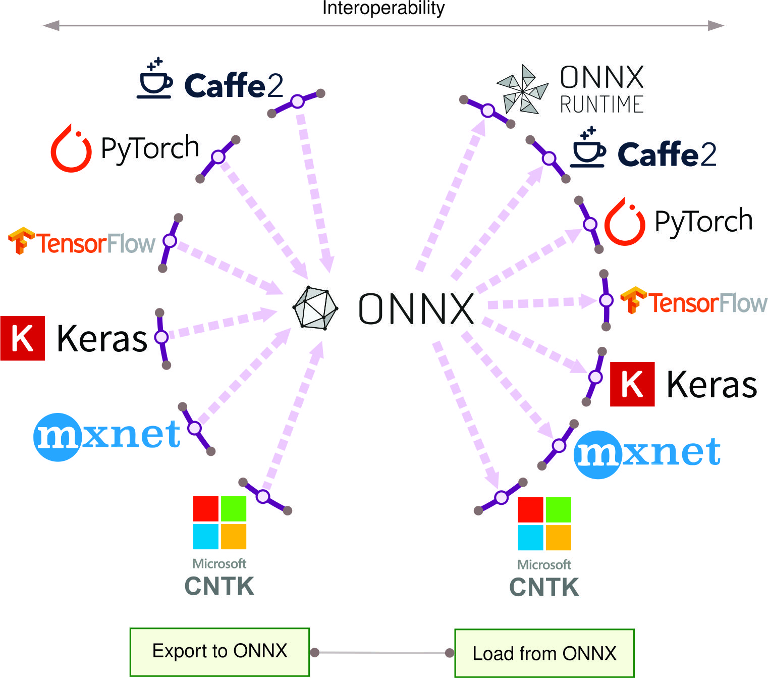
ONNX reduces the cost of framework fragmentation, but it does not eliminate the initial selection decision. The remaining question is how to choose a framework for a specific project’s constraints.
Self-Check: Question
When deploying deep learning models to microcontroller hardware (TinyML) with less than 256 KB of SRAM, which set of framework runtime assumptions is strictly required?
- Dynamic memory allocation via system malloc, full Python runtime, and 64-bit floating point precision
- Dynamic graph construction with autograd tape tracking enabled
- Cloud-based gRPC client with streaming RPC serialization
- Static memory allocation in a fixed pre-allocated arena, ahead-of-time compiled C/C++ kernels, 8-bit integer quantization, and zero dynamic memory allocation
Explain how the three core framework problems (Execution, Differentiation, Abstraction) are dramatically reweighted when transitioning from cloud model training to edge/embedded inference.
Explain how ONNX acts as a hub-and-spoke bridge between training frameworks and production inference engines, and identify the main systems risk when exporting complex models through ONNX.
Framework Selection
Framework selection is a constrained optimization problem across the same three framework problems. The question is not which framework is “best”; it is which execution model, differentiation system, and abstraction path survive the project’s constraints.
The framework selection trade-off space
Framework selection involves three interconnected tensions. The first is between development velocity and production performance: eager execution prioritizes iteration speed, while graph compilation prioritizes runtime optimization. Research teams that need to test ten architecture variants per day cannot afford minutes of compilation between experiments; production teams that deploy a single model for months cannot afford the throughput penalty of eager dispatch. The optimal point shifts as a project moves through its lifecycle.
This velocity-performance tension leads directly to the second, flexibility versus optimization depth. Eager execution makes host-language control flow natural but limits compiler scope until a larger region is captured. Static graphs can represent data-dependent control flow through graph operations while exposing more of the program for fusion and hardware-specific code generation. As table 3 demonstrated, this trade-off cascades through memory management, utilization, and debugging workflows. It is not a single design decision but a system-wide constraint.
The flexibility-optimization tension, in turn, exposes a third: ecosystem breadth vs. specialization. General-purpose frameworks cover broad operation sets but often underperform specialized runtimes on workloads those runtimes can optimize deeply. TensorRT, TVM, and similar systems optimize for narrower deployment targets through fusion, precision selection, and hardware-specific scheduling (NVIDIA 2024b; Chen et al. 2018). ONNX bridges part of this gap through standardized interchange (ONNX Contributors 2019). Runtime specialization still has to be evaluated separately: the more a runtime specializes, the more it depends on conversion coverage, supported operators, and fallback behavior.
NVIDIA. 2024b. NVIDIA TensorRT: Programmable Inference Accelerator.
Chen, Tianqi, Thierry Moreau, Ziheng Jiang, Lianmin Zheng, Eddie Q. Yan, Haichen Shen, Meghan Cowan, et al. 2018. “TVM: An Automated End-to-End Optimizing Compiler for Deep Learning.” Proceedings of the 13th USENIX Symposium on Operating Systems Design and Implementation (OSDI ’18), 578–94.
ONNX Contributors. 2019. ONNX: Open Neural Network Exchange.
Systems Perspective 1.4: Framework selection constraints
Rather than seeking the “best” framework, effective selection first eliminates candidates that cannot satisfy hard constraints: deployment target, required operations, compiler path, and team expertise. Only then should soft preferences such as performance, development speed, and ecosystem rank the survivors.
The TensorFlow ecosystem illustrates how these axes interact concretely. Its three variants (TensorFlow, TensorFlow Lite, TensorFlow Lite Micro) trace a single design philosophy across progressively tighter constraints, a pattern that generalizes to any framework family. Table 13 traces the trade-offs.
| TensorFlow | TensorFlow Lite | TensorFlow Lite for Microcontrollers | |
|---|---|---|---|
| Training | Yes | Limited | No |
| Inference | Yes | Yes | Yes |
| Operator Coverage | Broad | Inference-focused | Model-selected subset |
| Native Lower-Precision Tooling | Yes | Yes | Yes |
The principle is progressive constraint leading to progressive optimization: fewer supported operations enable smaller binaries, tighter memory budgets, and deployment-focused lower-precision execution. Three dimensions structure this analysis: model requirements define the supported operations, software dependencies define the runtime environment, and hardware constraints define the physical limits.
Framework selection criteria
Three dimensions structure systematic framework evaluation: what the model requires (supported operations and graph semantics), what the software environment provides (OS, memory management, accelerator delegation), and what the hardware physically permits (compute, memory, power). Each dimension acts as a filter: hard constraints eliminate candidates, and soft preferences rank the survivors.
Model requirements
The first question is whether a framework can express the models a project requires. Examine table 13. Operator coverage narrows from full TensorFlow to TensorFlow Lite and then to the model-selected subset linked into TensorFlow Lite Micro. Each reduction narrows training capability and general-purpose operations while concentrating deployment tooling. The engineering principle is that algorithmic expressiveness and machine efficiency trade against each other. Fewer supported operations enable tighter code generation, smaller binaries, and hardware-specific optimization paths. This progressive constraint model applies to any framework family, not just TensorFlow. Layered on top of operator coverage is a separate axis with its own trade-off, whether the graph is captured statically before execution or assembled dynamically at runtime.
Systems Perspective 1.5: Dynamic vs. static computational graphs
The static-vs.-dynamic graph distinction (examined in section 1.3) has direct implications for model requirements analysis. Static graphs require control flow and dynamic behavior to be represented in forms understood by the graph runtime, which enables ahead-of-time optimization for deployment. Eager execution follows ordinary Python control flow directly, while graph-capture paths such as
torch.compile and tf.function recover optimization opportunities when they can represent the executed program.
Software dependencies
Once model requirements are satisfied, the framework must integrate with the target software environment. Table 14 reveals how operating system requirements, memory management, and accelerator support vary across TensorFlow variants.
| TensorFlow | TensorFlow Lite | TensorFlow Lite for Microcontrollers | |
|---|---|---|---|
| Needs an OS | Yes | Yes | No |
| Model Access | Filesystem or service | Platform-specific storage mapping | Platform-specific compiled or mapped storage |
| Accelerator Support | Yes | Delegates | Optimized kernels and integrations |
The key distinctions follow the same progressive constraint pattern. TensorFlow Lite Micro eliminates the OS requirement entirely, enabling bare-metal execution on microcontrollers (though it integrates with RTOSes like FreeRTOS and Zephyr when available). How each Lite runtime accesses a model depends on the platform and integration. TensorFlow Lite uses delegates for supported accelerators, while TensorFlow Lite Micro can use platform-optimized DSP or accelerator kernels without the standard delegate mechanism. Each software dependency removed is a deployment target gained.
Hardware constraints
Software compatibility alone does not guarantee deployment; the framework must fit within physical hardware limits. Table 15 sets out this final constraint dimension.
Binary size and memory footprint depend on the selected build, operators, delegates, model, and runtime configuration. Processor architecture support shifts from x86 processors, GPUs, and TPUs in data centers through Arm Cortex-A platforms at the mobile/edge tier to Arm Cortex-M processors, DSPs, and MCUs in embedded systems. These are not arbitrary engineering tiers—they mirror the physical constraints (Light Barrier, power wall, memory wall) that carve the deployment spectrum into distinct paradigms (Physical Constraints: Why Paradigms Exist). The engineering lesson generalizes beyond TensorFlow: every framework family that spans deployment tiers makes analogous trade-offs between capability and resource footprint, and the framework’s job is to make those trade-offs navigable rather than invisible.
| TensorFlow | TensorFlow Lite | TensorFlow Lite for Microcontrollers | |
|---|---|---|---|
| Base Binary Size | Build- and package-dependent | Build- and delegate-dependent | Model- and operator-selection-dependent |
| Base Memory Footprint | Model-, runtime-, and allocator-dependent | Model-, delegate-, and allocator-dependent | Fixed arena plus runtime state |
| Optimized Architectures | x86, TPUs, GPUs | Arm Cortex-A, x86 | Arm Cortex-M, DSPs, MCUs |
Production-ready evaluation factors
Beyond this expressiveness-efficiency trade-off, technical specifications establish necessary but not sufficient conditions for selection. Production deployments also require evaluating migration cost, maintenance burden, and deployment reliability.
These hardware constraints cascade into tightly coupled performance trade-offs. Inference latency, memory footprint, power consumption, and hardware utilization depend on the model and target device rather than on the runtime family alone. Lower-precision execution can reduce memory, latency, and energy at the cost of numerical margin, and framework selection determines which optimization levers are available. Scalability introduces a further concern. Consistent deployment from microcontrollers to servers, smooth prototype-to-production transitions, and version management across deployed fleets all depend on the framework’s deployment toolchain. The three-dimension methodology illustrated here (model requirements, software dependencies, and hardware constraints) applies to any framework ecosystem, not just TensorFlow.
Development support and long-term viability assessment
Framework viability over a five-year production deployment depends on whether the ecosystem keeps the chosen execution, differentiation, and abstraction paths maintainable. Community composition matters because it determines which problems receive engineering attention: research-heavy ecosystems tend to improve experimentation and reproducibility first, production-heavy ecosystems tend to improve serving, monitoring, and compatibility first, and smaller specialized ecosystems tend to advance narrower mathematical or compiler capabilities faster than broad deployment tooling.
A framework’s practical utility often depends more on these surrounding paths than on the core tensor API. Model hubs, experiment trackers, serving runtimes, cloud ML services, and interchange formats can reduce lock-in or deepen optimization, but each also adds a dependency that must be maintained. These compounding effects make framework migration progressively harder: CI/CD pipelines, monitoring infrastructure, cloud integrations, and custom operators turn an API choice into an operational commitment. The measurable indicators of viability are therefore contributor diversity, backward compatibility track record, available hiring pool, and the cost of preserving an exit path through standardized formats such as ONNX, framework-agnostic data pipelines, and documented customizations.
The three core problems have so far appeared in isolation: execution, differentiation, and abstraction examined one at a time, with framework choices and selection criteria layered on top. A single training step is where the three problems collide. Tracing one end-to-end reveals how framework execution, differentiation, and hardware abstraction operate as one integrated system.
Self-Check: Question
An engineering team is architecting a new commercial computer vision system. In the chapter’s decision framework, why must deployment constraints (e.g. target mobile NPU delegates and memory budgets) act as hard filters evaluated before selecting the training framework?
- If a training framework cannot export or compile the required model operators to the target deployment runtime, the model cannot run in production regardless of its training speed or developer ergonomics
- Training frameworks automatically alter target hardware specifications to match model requirements
- Hard deployment filters guarantee that the model achieves 100% classification accuracy
- Research iteration speed is the only metric that matters in commercial system design
When evaluating framework viability for a production system expected to operate for 5+ years, which factor represents the greatest long-term architectural risk?
- Using Python instead of Fortran for high-level model definitions
- Adopting a niche or abandoned framework with dwindling maintainer support, which risks broken compiler toolchains, lack of support for new accelerator chips, and forced legacy stack maintenance
- Selecting an open-source framework backed by major hardware vendors
- Training on GPU clusters rather than single CPU workstations
Describe the three fundamental tensions in the framework selection trade-off space (velocity vs. performance, flexibility vs. optimization depth, ecosystem breadth vs. specialization).
True or False: Because model weights are stored as floating-point arrays, an engineering team can choose any training framework for research and assume that converting to a production embedded runtime is a trivial format conversion step.
Anatomy of a Training Step
Eight executable Python statements make eager vs. graph execution, reverse-mode autodiff, tensor abstractions, and kernel dispatch interact inside a single training step. Tracing that step through the PyTorch stack reveals how the execution, differentiation, and abstraction machinery operate simultaneously.
Listing 29 presents a minimal training iteration for a two-layer multilayer perceptron. Though only eight executable statements, this code exercises the entire framework stack: tensor allocation, kernel dispatch, autograd recording, gradient computation, and parameter updates. Tracing each phase reveals the three problems in action and connects the quantitative principles developed in section 1.1 to concrete execution.
# Single training step for a 2-layer MLP
x = torch.randn(32, 784, device="cuda")  # Input batch
y = torch.randint(0, 10, (32,), device="cuda")  # Labels

# Forward pass
optimizer.zero_grad()
h = torch.relu(x @ W1 + b1)  # Hidden layer
logits = h @ W2 + b2  # Output layer
loss = F.cross_entropy(logits, y)

# Backward pass
loss.backward()

# Parameter update
optimizer.step()
Phase 1: Forward pass (solving the execution problem)
During the forward pass, when h = torch.relu(x @ W1 + b1) executes, PyTorch’s eager execution triggers immediate computation:
- Python dispatch: The Python interpreter calls
torch.matmul, which routes through PyTorch’s dispatcher to select the CUDA backend, adding microseconds-scale overhead before device work begins. - Kernel selection: cuBLAS selects an optimized GEMM kernel based on matrix dimensions (32 \(\times\) 784 \(\times\) 256). For these dimensions, it might choose a tiled algorithm optimized for L2 cache.
- Kernel launch: The selected kernel is queued to the GPU’s command buffer, adding a few microseconds of launch overhead while the CPU continues immediately through asynchronous execution.
- GPU execution: The kernel loads W1 from HBM29 to L2 cache, performs the matrix multiply in Tensor Cores when available, and writes the result back to HBM; for this small GEMM, the workload usually still lasts only microseconds.
- Autograd recording: Simultaneously, PyTorch’s autograd engine records a
MmBackwardnode on the tape, storing references toxandW1for gradient computation.
29 HBM (high bandwidth memory): Provides 2–3 TB/s bandwidth on modern GPUs, making it the memory tier that most directly feeds accelerator arithmetic; HBM bandwidth determines whether operations are memory bound or compute bound, and its 80 GB capacity on an A100 sets the hard ceiling on total live training state. Weights, activations, gradients, optimizer state, and temporary workspace must fit during execution. When they do not, the framework must resort to offloading, selective recomputation, or placement across devices, each adding complexity to what the programmer perceives as a single loss.backward() call.
The bias addition and ReLU follow similar patterns, each adding a node to the autograd tape.
Phase 2: Backward pass (solving the differentiation problem)
Calling loss.backward() triggers a four-stage backward pass:
- Tape traversal: The autograd engine traverses the recorded graph in reverse topological order.
- Gradient Computation: For each node, it calls the registered backward function, where \(W_1\) and \(W_2\) are layer weight matrices that form part of the model parameters \(\theta\). Traversing in reverse,
CrossEntropyBackwardcomputes \(\frac{\partial \mathcal{L}}{\partial \text{logits}}\) using the softmax derivative;MmBackwardfor \(W_2\) computes \(\frac{\partial \mathcal{L}}{\partial W_2} = h^T \cdot \frac{\partial \mathcal{L}}{\partial \text{logits}}\) along with \(\frac{\partial \mathcal{L}}{\partial h}\);ReluBackwardapplies the ReLU derivative mask (zero where \(h \leq 0\)); andMmBackwardfor \(W_1\) computes \(\frac{\partial \mathcal{L}}{\partial W_1}\). The example does not request a gradient for the input tensorx. - Gradient Accumulation: Gradients are accumulated into
.gradattributes of leaf tensors. - Memory Management: Once a backward node’s saved tensors are no longer needed and no other references retain them, the framework can release that state for memory reuse.
Together, these backward-pass stages turn the recorded forward graph into gradients while releasing intermediate state as soon as it is no longer needed.
Phase 3: Memory traffic analysis (the physics at work)
Applying equation 4 to this step, table 16 breaks down the FLOPs, memory traffic, and arithmetic intensity for each operation:
| Component | Modeled Work | Memory Traffic | Arithmetic Intensity |
|---|---|---|---|
| MatMul (x @ W1) | \(2 \times 32 \times 784{\times}256\) = 12.8 MFLOP | 0.9 MB | 13.7 FLOP/byte |
| ReLU | \(32{\times}256\) = 8.2 KFLOP | 65.5 KB | 0.125 FLOP/byte |
| MatMul (h @ W2) | \(2 \times 32 \times 256{\times}10\) = 163.8 KFLOP | 44.3 KB | 3.7 FLOP/byte |
| Cross-entropy (simplified) | ~0.96 KFLOP | 2.6 KB | 0.4 FLOP/byte |
| Backward (assumed 2\(\times\) forward) | ~26 MFLOP | 3.1 MB | 8.3 FLOP/byte |
The arithmetic-intensity column is the diagnostic column. Matrix multiplications reuse operands enough to move toward the compute roof, while ReLU and cross-entropy move too little work per byte to escape the memory and launch-overhead regime. This is why fusion and dispatch reduction matter even when the model is written in high-level tensor code.
The model estimates ~39.1 MFLOP of work and ~4.2 MB of memory traffic. To obtain ideal lower bounds, we divide these estimates by the A100 peak rates:
- \(T_{\text{compute}} \approx\) 39.1 MFLOP/19.5 TFLOP/s FP32 ≈ 2.0 μs
- \(T_{\text{memory}} \approx\) 4.2 MB/2.04 TB/s ≈ 2.1 μs
- Assuming 12 ops kernel launches, \(T_{\text{overhead}} \approx\) 12 ops \(\times\) 15 μs ≈ 180 μs
Under the stated launch-count and per-launch assumptions, the modeled training step is overhead-bound. Small models are often sensitive to Python dispatch and kernel launch costs, which drives three common production practices that all serve to reduce the dispatch term rather than changing the model’s mathematical work:
torch.compilecan speed favorable small-operation workloads by fusing operations and reducing kernel launches- Batch size increases help amortize per-batch overhead
- Larger, compute-dense operations can amortize dispatch overhead
Phase 4: Hardware abstraction (solving the abstraction problem)
The same Python code runs on different hardware through abstraction layers, each pairing a backend library with a hardware-specific execution mechanism, as table 17 summarizes.
Each backend implements common tensor-operation semantics with hardware-specific optimizations. A single loss.backward() call can therefore trigger different code paths depending on the hardware. Floating-point precision, reduction order, kernel selection, and nondeterministic operations may produce numerical differences across backends, so equivalence must be evaluated within the framework’s documented tolerances and determinism guarantees.
| Hardware | Backend library | Execution mechanism |
|---|---|---|
| CUDA GPU | cuBLAS (NVIDIA 2024a; Choquette et al. 2021) | GEMM kernels and CUDA streams for async execution |
| CPU | Intel oneMKL or OpenBLAS (Intel Corporation 2026; OpenBLAS Project 2026) | Thread-level parallelism around optimized kernels |
| TPU | XLA (Google 2025) | Compilation to TPU-specific high-level optimizer (HLO) operations |
| Apple Silicon | Metal Performance Shaders | MPS backend |
Choquette, Jack, Wishwesh Gandhi, Olivier Giroux, Nick Stam, and Ronny Krashinsky. 2021. “NVIDIA A100 Tensor Core GPU: Performance and Innovation.” IEEE Micro 41 (2): 29–35. https://doi.org/10.1109/mm.2021.3061394.
Intel Corporation. 2026. Intel oneAPI Math Kernel Library.
OpenBLAS Project. 2026. OpenBLAS: An Optimized BLAS Library.
Google. 2025. XLA: Optimizing Compiler for Machine Learning.
This detailed trace through a single training step demonstrates how deeply the three core problems interact. Even simple code exercises the full framework stack, and seemingly minor decisions—device placement, batch size, compilation mode—cascade through execution, differentiation, and abstraction layers in ways that are difficult to predict without systems-level understanding. The pitfalls that follow are the common failure modes when that systems view is missing.
Systems Perspective 1.6: The three problems in action
This trace reveals the three problems in concrete terms:
- Execution: Eager mode enables line-by-line debugging but incurs dispatch overhead
- Differentiation: Autograd tape records operations during forward, replays in reverse during backward
- Abstraction: Same code runs on GPU/CPU/TPU through backend-specific kernel implementations
Understanding this flow enables informed optimization: fuse operations to reduce overhead, use appropriate batch sizes, and match model scale to hardware capabilities.
Self-Check: Question
During the forward execution of an MLP layer
h = torch.relu(x @ W1 + b1)withrequires_grad=True, what two operations occur concurrently inside the framework?- It computes the forward output and immediately updates the weights
W1using gradient descent - It executes the matrix multiplication on the GPU and transmits the gradients back to the host CPU
- It computes the forward numerical activations on the hardware accelerator and constructs a dynamic autograd tape recording the operations and caching required intermediate tensors for the backward pass
- It compiles the entire Python script into a native standalone mobile application
- It computes the forward output and immediately updates the weights
In the chapter’s training step roofline analysis on an NVIDIA A100 GPU, the raw compute and memory transfer time for a 2-layer MLP batch takes ~4 \(\mu\text{s}\), but total eager-mode execution takes ~30–50 \(\mu\text{s}\). What systems bottleneck explains this discrepancy?
- Network congestion across distributed InfiniBand interconnects
- Thermal throttling of the GPU streaming multiprocessors
- Memory leakage inside the PyTorch dynamic class hierarchy
- CPU dispatch overhead, where launching ~12 separate small kernels across Python and CUDA runtimes incurs ~2–5 \(\mu\text{s}\) of launch latency per operation
Contrast the arithmetic intensity of a matrix multiplication (
MatMul) with an element-wise activation function (ReLU) in a neural network layer, and explain why their performance bottlenecks differ fundamentally on modern GPUs.Order the complete sequence of computational and system phases occurring inside a framework during a single standard training iteration:
Loss calculation: The criterion function evaluates the scalar training loss \(\mathcal{L}\)
Backward pass: Autograd traverses the reverse tape, executing Vector-Jacobian Products and populating
.gradbuffersOptimizer step: The optimizer reads
.gradvalues and updates parameter tensors in-place using the optimization algorithmForward pass: The model executes layer operations and records the dynamic autograd tape
Gradient reset:
optimizer.zero_grad()clears or sets.gradbuffers toNoneDuring the backward pass of a training step, why is memory traffic often significantly higher than in the forward pass, even though the number of mathematical operations is roughly comparable?
Fallacies and Pitfalls
Framework selection involves subtle trade-offs where intuitions from conventional software engineering fail. The memory wall, kernel fusion constraints, and deployment target diversity create pitfalls that waste engineering effort and cause production systems to miss latency targets.
Fallacy: “All frameworks provide equivalent performance for the same model architecture.”
Engineers assume that ResNet-50 yields identical performance across frameworks since the mathematics is the same, forgetting that performance is an emergent property of algorithm-machine co-design. In production, implementation matters. Compiled execution can improve supported eager workloads, and hardware-specialized inference engines such as TensorRT or TVM can reduce latency relative to untuned eager baselines when conversion is clean. The difference arises from kernel fusion depth, graph optimization strategies, memory access patterns, precision support, and backend libraries that vary between frameworks. Organizations that assume equivalence can miss latency service level agreements and require costly last-minute framework migrations.
Pitfall: Choosing frameworks based on popularity rather than project requirements.
Engineers assume the most popular framework works for any project. In reality, deployment constraints dominate. A mobile runtime such as ExecuTorch or TensorFlow Lite and a microcontroller runtime such as TensorFlow Lite Micro make different assumptions about memory allocation, operator coverage, and hardware delegates; the former targets phones with GB-scale memory, while the latter often targets devices with hundreds of KB of RAM, commonly below 256 KB for small TinyML deployments. Teams that prototype edge applications without checking the final runtime can face memory bloat that exceeds device capacity or a late framework migration after development completes. Evaluate deployment targets per section 1.8 before selecting a training framework.
Fallacy: “Framework abstractions eliminate the need for systems knowledge.”
Engineers assume high-level APIs handle all optimization automatically. The Roofline Model (The Roofline model) proves otherwise. Element-wise operations such as ReLU perform little arithmetic per byte moved, so memory traffic and launch overhead can dominate even on accelerators with abundant compute. Section 1.3.1 explains how this imbalance can leave compute resources idle. Engineers must identify the limiting resource before choosing fusion, batching, layout, or precision optimizations.
Pitfall: Ignoring vendor lock-in from framework-specific formats.
Engineers assume framework migration is straightforward since models are “just math.” Converting TensorFlow SavedModel to PyTorch can require rewriting custom operations, validating numerical equivalence across large test suites, and retraining when operations lack exact equivalents. ONNX (section 1.8) improves portability, but custom operators, dynamic shapes, and backend-specific optimizations can still require manual work. Organizations that ignore this during initial framework selection face costly migrations when deployment requirements change or better frameworks emerge.
Fallacy: Training framework choice is independent of production infrastructure.
Engineers assume training framework choice is independent of deployment infrastructure. In practice, framework-infrastructure mismatches can impose substantial operational overhead. Some serving stacks provide atomic model swaps, while others require a process or container restart unless the deployment architecture adds version routing around them. Some frameworks and runtimes expose monitoring hooks directly; others require custom instrumentation. These are preview consequences of the serving and operations layers developed in Model Serving and ML Operations; the local lesson is to evaluate the complete deployment stack during framework selection, including serving infrastructure, monitoring, and operational tooling.
Pitfall: Increasing batch size without modeling activation memory.
Engineers assume that if memory is available, larger batches always improve throughput. Larger mini-batches can amortize fixed dispatch overhead, but they also scale the activation memory that must remain live during training. A 7-billion-parameter model in FP16 consumes 14 GB, leaving 71.9 GB on an 80 GB A100 before accounting for other training state. Increasing batch size from 8 to 32 quadruples the batch-dependent activation footprint; transformer attention adds a large \(\mathcal{O}(S^2)\) term in sequence length that makes each sample expensive. The resulting memory pressure can trigger recomputation strategies whose additional work reduces throughput despite the larger batch. Teams that blindly maximize batch size can achieve lower throughput than smaller batches that avoid these memory management pathways; Gradient-based optimization methods formalizes the throughput target.
Fallacy: Compilation overhead is negligible.
Engineers assume compilation overhead is a one-time cost that pays off quickly. The hypothetical values in table 4 assign ResNet-50 higher compiled throughput and a compile window of 15 s to 30 s per graph change. Under those assumptions, a 10,000-image experiment with 10 code changes completes in 6.9 s in eager mode and 304.7 s in compiled mode, including recompilation overhead. The compiled workflow is therefore about 44.2× slower in this illustrative rapid-prototyping scenario. Teams that enable compilation during rapid prototyping can waste time waiting for recompilations that negate throughput gains.
Pitfall: Using one execution policy for exploration and production.
The right framework mode depends on the loop. During exploration, eager execution and small tests shorten feedback by avoiding repeated graph captures and recompilations. During production serving or long training runs, compilation can amortize setup across many requests or samples. The deciding factors are workload duration and stability: compilation pays when graph structure and shapes recur, whereas changing control flow or input shapes can invalidate cached artifacts and restart the amortization. Teams should choose the policy from measured iteration latency and steady-state throughput. One policy for both phases either slows research iteration or leaves production throughput unused.
Self-Check: Question
A research team exploring architecture modifications runs experiments where model code changes every 10 training steps. When they enable JIT graph compilation (
torch.compile), total training time increases by 5\(\times\) compared to standard eager mode. What systems principle explains this performance degradation?- Compilation incurs a large upfront compilation latency (\(T_{\text{compile}}\)); if graph structures or tensor shapes change frequently, the compilation cost cannot be amortized across executions (\(N_{\text{steps}} \times (T_{\text{eager}} - T_{\text{compiled}}) < T_{\text{compile}}\)), making repeated recompilation slower than eager execution
- Compiled kernels run at half the floating-point clock frequency of eager kernels on NVIDIA GPUs
- JIT compilers disable GPU hardware acceleration when running short training scripts
- Dynamic graph compilation automatically converts all FP32 operations to 64-bit double precision
Explain why choosing a framework based on community popularity or GitHub stars rather than binding deployment constraints is a severe engineering pitfall for edge and embedded ML projects.
True or False: Because standard neural network architectures (like ResNet-50 or Transformers) have identical mathematical definitions, any two frameworks running the same model on identical GPU hardware will produce identical throughput.
Summary
Machine learning frameworks exist to solve three fundamental problems that would otherwise make deep learning impractical. The first is execution: deciding when and how computation runs. Frameworks navigate the trade-off between eager execution (immediate, debuggable, flexible) and graph execution (deferred, optimizable, deployable), while modern hybrid approaches like torch.compile attempt to provide both flexibility during development and optimization for production. The second is differentiation: computing gradients automatically. Frameworks implement reverse-mode automatic differentiation that applies the chain rule across supported operation compositions, producing derivatives subject to floating-point arithmetic and each operation’s derivative rule. This software primitive makes training billion-parameter models possible through a loss.backward() call. The third is abstraction: targeting diverse hardware from a single interface. Frameworks provide tensor abstractions, intermediate representations, and runtime systems that hide hardware complexity while enabling efficient utilization across CPUs, GPUs, TPUs, and specialized accelerators.
These problems are interconnected and constrained by the iron law of performance (Iron Law of ML Systems): execution strategy determines dispatch overhead \((L_{\text{lat}})\), differentiation determines memory traffic \((D_{\text{vol}})\), and abstraction determines hardware utilization \((\eta_{\text{hw}})\). The memory wall can make data movement more expensive than computation, explaining why frameworks invest in kernel fusion, selective recomputation, lower-precision execution, and compilation pipelines.
Key Takeaways: The layer between math and hardware
- Every framework solves three problems: Execution determines how to run, differentiation how to train, and abstraction how to express. TensorFlow couples graph capture to broad deployment paths, PyTorch couples eager iteration to capture and export paths, and JAX organizes differentiation and compilation as composable function transformations. These are infrastructure commitments, not tooling preferences.
- The memory wall drives optimization: Compute capacity has grown far faster than memory bandwidth for decades, widening the cumulative gap that bounds data movement. Kernel fusion, selective recomputation, lower-precision execution, and data layout optimizations all target the data movement term \((D_{\text{vol}})\) in the iron law, not the compute term.
- Compilation must amortize setup cost: The compilation continuum principle in equation 2 quantifies when execution savings exceed compilation costs. Rapidly changing graphs often favor eager mode, while repeatedly executed stable graphs can benefit from progressive compilation from JIT to AOT. The dispatch overhead law in equation 4 explains why small operations can benefit disproportionately once compilation is reused.
- Module abstractions automate state management: Automatic parameter discovery, mode-dependent behavior, and hierarchical composition with serialization appear across major frameworks, enabling million-parameter optimization in a single optimizer step regardless of API syntax.
- Deployment constraints should drive selection: Inference engines, mobile runtimes, and microcontroller runtimes trade off operator coverage, memory allocation, compilation, and acceleration differently. Gaps between eager and specialized inference, or between server and microcontroller memory, are architectural constraints. Evaluate the deployment target before selecting a framework.
Understanding framework internals transforms how practitioners approach performance debugging and optimization. When a training job runs slower than expected, engineers who understand execution graphs can identify whether the bottleneck lies in eager-mode overhead, insufficient kernel fusion, or suboptimal memory layout. When deployment fails on target hardware, the compilation pipeline reveals whether the issue is operator support, quantization compatibility, or runtime configuration. This knowledge is essential for diagnosing and resolving performance issues in production systems.
A framework presents itself as a convenience, a cleaner way to write a model, and that is exactly what makes its influence easy to miss. Its real work is to translate mathematics into machine operations, and no translation is free: every choice it makes (eager or graph execution, when to fuse kernels, what precision to keep, how much to compile) shifts cost between the terms of the iron law rather than removing it. What looks like an API is therefore a standing decision about where the system will spend, made mostly before the engineer arrives. The framework cannot lighten the load the iron law names; it can only decide which of the three terms will carry it.
What’s Next: From control room to power plant
Frameworks are the software substrate that translates abstract architectures into executable kernels. Computational graphs, autograd tapes, and kernel dispatch pipelines are the control room instruments: they give engineers visibility into and control over the training process. The machinery is built, but every budget decision it exposes remains unmade: which activations to checkpoint when memory runs short, how large a batch the hardware allows, and at what point a single device stops being enough. Model Training is where those bills come due, scaling framework execution, differentiation, and memory-management machinery into the training systems that power modern AI.
Self-Check: Question
How do the three fundamental framework problems (Execution, Differentiation, Abstraction) map directly to the terms of the systems iron law (\(T_{\text{epoch}} = \frac{\text{Work}}{\text{Throughput}} \times \frac{1}{\eta_{\text{hw}}} + \text{Overhead}\))?
- Execution controls dataset size, differentiation controls network latency, and abstraction controls cloud server pricing
- All three problems affect only the floating-point precision of the weights
- Execution affects differentiation, while abstraction has no measurable impact on systems performance
- Execution strategy governs dispatch latency and kernel launch overhead (\(L_{\text{lat}}\)), differentiation governs intermediate activation memory volume and traffic (\(D_{\text{vol}}\)), and hardware abstraction governs silicon utilization efficiency (\(\eta_{\text{hw}}\))
Summarize why the memory wall—rather than raw floating-point arithmetic capacity—has become the primary driver of modern ML framework compiler innovations (such as kernel fusion and activation checkpointing).
True or False: An ML framework can eliminate the physical constraints imposed by the iron law of performance if an engineer writes clean, high-level declarative Python code.
Self-Check Answers
Self-Check: Answer
A team reports that their model executes correctly on CPU but produces mismatched tensor shapes and silent numerical corruption when switched to a GPU backend because some operators silently default to a different memory layout (such as NCHW versus NHWC). Which of the three fundamental framework problems does this failure most directly expose?
- The hardware abstraction problem, because one unified model interface must preserve consistent semantic behavior, memory layouts, and numerical contracts across diverse hardware backends
- The execution problem, because the operators were evaluated eagerly instead of being captured into a static graph
- The differentiation problem, because the backward pass failed to propagate gradients through non-contiguous strides
- A data engineering pipeline defect unrelated to framework runtime responsibilities
Answer: The correct answer is A. The hardware abstraction problem requires providing a unified interface across diverse hardware backends (CPUs, GPUs, TPUs) while ensuring consistent semantics, memory layouts, and numerical behaviors; a silent layout mismatch between backends is a direct failure of this abstraction. Blaming the execution problem confuses when operations are dispatched with how backends interpret tensor memory contracts. Attributing the issue to differentiation is incorrect because forward shape and layout divergences break before gradient propagation occurs. Dismissing it as a data pipeline defect overlooks that tensor layout conversion across backends is a core runtime responsibility.
Learning Objective: Classify a concrete framework failure into the execution, differentiation, or hardware abstraction problem
Explain how viewing an ML framework as a compiler for the silicon contract—rather than merely a numerical library like NumPy—changes an engineer’s expectations regarding framework selection and optimization under the systems iron law.
Answer: A numerical library executes individual operations immediately in isolation, where switching libraries primarily changes syntax without altering underlying execution. An ML framework acts as a compiler that translates an abstract computational graph into a physical execution plan, performing operator fusion, memory planning, and hardware-specific lowering. Consequently, framework selection sets an upper bound on achievable silicon efficiency and directly determines how effectively the system attacks the data movement (\(D_{\text{vol}}\)) and dispatch latency (\(L_{\text{lat}}\)) terms of the iron law.
Learning Objective: Explain how the compiler analogy changes an engineer’s expectations of what framework choice determines
True or False: Two frameworks that expose nearly identical user-facing Python tensor APIs and target the same GPU hardware will necessarily provide equivalent graph-level operator fusion and ahead-of-time compilation capabilities.
Answer: False. Syntactic API similarity does not imply compiler equivalence: one framework may support aggressive whole-graph intermediate representation lowering and kernel fusion via JIT/AOT compilers, whereas another may only perform eager single-kernel dispatch on the same GPU backend, resulting in substantial workload-dependent throughput gaps.
Learning Objective: Evaluate the misconception that matching tensor APIs imply matching compiler optimization capabilities
An engineering organization chose a specialized research framework for rapid prototyping, only to discover later that the framework lacks export paths to their production edge accelerators, requiring months of manual re-implementation. Applying the chapter’s infrastructure-commitment principle, what is the key systems insight?
- Framework choice is easily reversible because weight arrays can be loaded into any runtime with zero engineering overhead
- Framework selection functions as a durable infrastructure commitment whose reversal cost compounds across model checkpoints, serving runtimes, CI/CD pipelines, and hardware access
- The primary failure was selecting an overly compact model architecture that failed to saturate edge accelerator memory
- Hardware abstraction layers eliminate all differences between training frameworks and production inference engines
Answer: The correct answer is B. Framework decisions constrain reachable hardware targets, optimization passes, and deployment toolchains, meaning migration costs extend far beyond model code to include checkpoints, serving systems, CI/CD pipelines, and team expertise. Treating framework choice as freely reversible ignores the substantial engineering friction of cross-runtime translation. Blaming model capacity misidentifies the root cause, which is export toolchain incompatibility. Claiming hardware abstraction eliminates all deployment differences ignores real-world operator coverage gaps and runtime constraints.
Learning Objective: Analyze why framework selection functions as a long-term infrastructure commitment rather than a reversible tooling choice
Self-Check: Answer
While NumPy provided high-performance linear algebra by wrapping BLAS in Python, what critical scaling bottleneck did it leave unaddressed that motivated the development of deep learning frameworks such as Theano, TensorFlow, and PyTorch?
- Inability to execute matrix multiplications on single-core CPU architectures
- Lack of an \(n\)-dimensional array data structure in scientific computing
- The requirement for manual gradient derivation and hand-written backpropagation passes for multi-layer neural networks
- Inability to run compiled Fortran and C routines through high-level scripting languages
Answer: The correct answer is C. NumPy provided high-level array ergonomics and BLAS-backed performance, but practitioners still had to manually derive and implement analytical backpropagation gradients, creating an error-prone bottleneck for deep networks that automatic differentiation frameworks solved. Single-core CPU matrix multiplication was already solved at the BLAS layer. The \(n\)-dimensional array abstraction was NumPy’s primary feature rather than a missing capability. Python-to-C/Fortran bindings were the core mechanism of NumPy’s vectorization model rather than an unsolved problem.
Learning Objective: Analyze which scaling bottleneck NumPy left open for subsequent deep learning frameworks to solve
Explain why the relationship between rungs on the ladder of abstraction (such as BLAS/LAPACK, NumPy, and modern deep learning frameworks) is characterized by inheritance rather than replacement.
Answer: Higher rungs on the ladder do not replace the numerical primitives of lower rungs; instead, they wrap and orchestrate them while automating higher-level concerns such as automatic differentiation, memory planning, and graph compilation. For instance, a high-level PyTorch matrix multiplication
torch.matmul(A, B)ultimately delegates to vendor-optimized BLAS kernels (such as cuBLAS on NVIDIA GPUs), meaning an inefficient low-level primitive establishes a performance ceiling for all frameworks built above it.Learning Objective: Explain how successive ladder rungs inherit low-level primitives rather than replacing them
**Order the following historical computing milestones in the evolution of numerical and machine learning software abstractions, from earliest (1979) to most recent (2018):
JAX introduces functional composable transformations and XLA compilation
BLAS standardizes reusable low-level linear algebra primitives
Theano introduces compiled Python computational graphs for GPUs
NumPy establishes Python’s unified \(n\)-dimensional array and vectorization standard
PyTorch introduces dynamic define-by-run execution graphs
LAPACK extends BLAS with higher-level numerical routines (e.g., SVD, factorizations)**
Answer: The correct sequence is 2 -> 6 -> 4 -> 3 -> 5 -> 1:
- BLAS (1979): Standardized low-level linear algebra primitives.
- LAPACK (1992): Extended BLAS with higher-level matrix factorizations and numerical solvers.
- NumPy (2006): Unified Python scientific array abstractions and vectorized dispatch.
- Theano (2007): Introduced Python-defined symbolic computational graphs compiled to GPU code.
- PyTorch (2016): Popularized dynamic define-by-run computational graphs.
- JAX (2018): Introduced functional composable transformations (
grad,vmap,jit) backed by XLA.
- JAX (2018): Introduced functional composable transformations (
The architectural design pattern established by NumPy, where high-level control logic is written in an expressive interpreted language (such as Python) while inner numerical loops are delegated to compiled C/Fortran libraries, is known as ____.
Answer: The correct answer is vectorization (or vectorized execution). Vectorization allows developers to write clean array-level expressions in Python while delegating repetitive element-wise and matrix loops to optimized native code.
Learning Objective: Identify the vectorization design pattern that connects interpreted frontends to compiled numerical backends
Self-Check: Answer
A GPU performance profile reveals that a sequence of LayerNorm, dropout, and GELU activation operations spends over 80% of its execution time reading and writing intermediate tensors to High Bandwidth Memory (HBM) with very low arithmetic intensity. Why is operator fusion the primary framework optimization for this workload?
- It replaces 16-bit floating-point arithmetic with 8-bit integer arithmetic
- It changes the model architecture to eliminate all non-linear activation functions
- It converts compute-bound matrix multiplications into memory-bound operations
- It fuses multiple sequential element-wise operations into a single GPU kernel, keeping intermediate values in on-chip SRAM/registers and eliminating redundant round trips to HBM
Answer: The correct answer is D. Element-wise and normalization layers have low arithmetic intensity and are memory-bandwidth-bound; operator fusion combines these sequential passes into a single GPU kernel that passes intermediate values through fast on-chip registers and SRAM, drastically reducing global HBM memory traffic. Precision quantization changes numerical representation rather than performing fusion. Modifying network architecture mischaracterizes a compiler optimization as a model alteration. Converting operations to memory-bound would degrade rather than improve arithmetic efficiency.
Learning Objective: Analyze why operator fusion mitigates memory-wall bottlenecks for low arithmetic intensity layers
A developer attempts to trace a dynamic PyTorch model containing data-dependent control flow (
if tensor.sum() > 0: ...) using standard graph tracing (torch.jit.trace). What failure mode occurs, and how does modern bytecode graph capture (torch.compile/ TorchDynamo) resolve it?- Standard tracing crashes immediately on any tensor operation, whereas TorchDynamo rewires the Python interpreter into C++
- Standard tracing converts all dynamic control flow into static loops, whereas TorchDynamo disables all GPU acceleration
- Standard tracing records only the branch taken by the example input and silently bakes it into a static graph, whereas TorchDynamo inspects Python bytecode to capture straight-line subgraphs into FX graphs and falls back to the Python interpreter on graph breaks
- Standard tracing successfully compiles dynamic branches using AST inspection, whereas TorchDynamo rejects all conditional statements
Answer: The correct answer is C. Tracing executes the program with dummy inputs and records the executed trace, silently dropping untaken conditional branches; TorchDynamo intercepts Python frame evaluation bytecode, extracts valid computational subgraphs into FX graphs, and gracefully falls back to the Python interpreter (a graph break) when encountering unsupported dynamic constructs. Claiming tracing crashes on all tensor operations is factually incorrect. Asserting that tracing converts conditionals to static loops misrepresents trace capture. Suggesting tracing handles dynamic branches via AST confuses tracing with source-to-source compilers like TorchScript script mode.
Learning Objective: Compare graph tracing with bytecode frame interception for handling dynamic control flow
State the dispatch overhead law and explain why a workload composed of many small tensor operations on an NVIDIA A100 GPU can be severely underutilized in eager mode even if the GPU has massive compute throughput.
Answer: The dispatch overhead law states that a workload is overhead-bound when the overhead ratio \((N_{\text{ops}} \cdot t_{\text{dispatch}}) / (T_{\text{compute}} + T_{\text{memory}}) > 1\). Because eager execution incurs a CPU-to-GPU launch tax of ~\(2\text{--}5\ \mu\text{s}\) per operation, a small kernel executing in less than \(2\ \mu\text{s}\) forces the GPU to sit idle between launches, bottlenecking end-to-end throughput on CPU dispatch latency rather than GPU arithmetic capacity.
Learning Objective: Explain how the dispatch overhead law causes GPU underutilization on small eager-mode operations
True or False: In
torch.compile, encountering a “graph break” halts program execution and throws a fatal runtime exception because dynamic Python constructs cannot be represented in the computational graph.Answer: False. A graph break does not crash the program; instead, TorchDynamo captures the preceding operations as a compiled subgraph, safely falls back to the standard Python interpreter to execute the unsupported dynamic code, and then resumes graph capture for subsequent operations.
Learning Objective: Evaluate the operational behavior and performance impact of graph breaks in graph-capture JIT compilers
**Order the stages of the
torch.compilecompilation and execution pipeline in PyTorch 2.0, from initial Python function call to hardware execution:AOTAutograd traces both the forward and backward computation graphs ahead of execution
TorchDynamo intercepts Python bytecode during frame evaluation and extracts computational subgraphs
TorchInductor generates optimized vendor-specific kernels (e.g., Triton for GPUs or C++/OpenMP for CPUs)
The high-level intermediate representation is structured as a PyTorch FX graph
The compiled fused kernels execute on the target hardware accelerator**
Answer: The correct sequence is 2 -> 4 -> 1 -> 3 -> 5:
- TorchDynamo intercepts Python bytecode: Hooks frame evaluation to extract tensor operations.
- PyTorch FX graph generation: Produces a high-level Python-level intermediate representation.
- AOTAutograd tracing: Captures both forward and backward computational graphs.
- TorchInductor lowering: Compiles FX graphs into fused hardware-specific Triton/C++ kernels.
- Hardware execution: Dispatches the optimized kernels on the accelerator.
In graph-capture JIT compilation systems like TorchDynamo, an event where the compiler encounters an unsupported dynamic Python construct (such as an unhandled C-extension call or dynamic side effect) and must pause graph capture to yield control to the Python interpreter is called a ____.
Answer: The correct answer is graph break. A graph break splits the computational graph into multiple subgraphs separated by interpreted Python execution, which can increase kernel dispatch overhead.
Learning Objective: Identify the concept of a graph break in graph-capturing execution systems
Self-Check: Answer
For a neural network with \(N = 10^7\) parameters and a single scalar loss output \(M = 1\), why do deep learning frameworks uniformly employ reverse-mode automatic differentiation (backpropagation) instead of forward-mode differentiation?
- Reverse-mode computes all \(10^7\) parameter gradients in a single backward pass of complexity \(\mathcal{O}(M) = \mathcal{O}(1)\), whereas forward-mode would require \(10^7\) separate passes of complexity \(\mathcal{O}(N)\)
- Forward-mode differentiation cannot compute exact gradients and relies on finite-difference approximations
- Reverse-mode differentiation requires zero memory allocation for intermediate forward activations
- Forward-mode is restricted exclusively to non-linear activation functions and cannot differentiate matrix multiplications
Answer: The correct answer is A. Reverse-mode automatic differentiation (vector-Jacobian products) computes gradients of a scalar loss (\(M=1\)) with respect to all \(N\) input parameters in a single backward traversal with compute cost proportional to the forward pass, whereas forward-mode (Jacobian-vector products) scales with \(N\), requiring \(10^7\) forward passes. Forward-mode computes mathematically exact derivatives, not finite differences. Reverse-mode actually requires storing intermediate forward activations in memory, which is its primary drawback. Forward-mode applies to all differentiable operations including matrix multiplications.
Learning Objective: Calculate and compare the computational complexity scaling of forward-mode and reverse-mode automatic differentiation
A PyTorch user modifies an intermediate activation tensor using an in-place operation (
x.relu_()orx += 1) during the forward pass. Duringloss.backward(), autograd raises a runtime error: “one of the variables needed for gradient computation has been modified by an inplace operation”. What is the systems mechanism causing this failure?- In-place operations convert 32-bit floating point numbers to integers, corrupting floating-point precision
- The autograd tape recorded a reference to the forward tensor whose underlying storage was overwritten, destroying the original activation values required by the operation’s derivative formula
- In-place operations automatically set
requires_grad=Falseon all ancestor nodes in the computational graph - The GPU caching allocator prohibits in-place memory modifications during forward execution
Answer: The correct answer is B. Autograd saves pointers to intermediate activations during the forward pass via functions like
ctx.save_for_backward(); modifying those buffers in-place overwrites the numerical values needed to evaluate derivative formulas during the backward pass, triggering version-counter mismatch errors. In-place operations preserve data types and do not convert floats to integers. In-place operations do not alter therequires_gradflags of ancestor nodes. The hardware memory allocator does not restrict in-place buffer mutations; the error is enforced by framework autograd version tracking.Learning Objective: Analyze why in-place tensor mutations break autograd tape integrity during reverse-mode differentiation
Explain the difference between accumulating gradients in a tensor’s
.gradattribute across batches and retaining the autograd computational graph usingloss.backward(retain_graph=True).Answer: Gradient accumulation adds new derivative values into existing parameter
.gradbuffers (param.grad += dL/dParam), which is a lightweight numerical addition that allows simulating larger batch sizes. In contrast,retain_graph=Trueprevents autograd from freeing the intermediate activation tensors andGradFngraph nodes after the backward pass, keeping them pinned in memory and potentially causing GPU Out-Of-Memory errors if retained across iterations.Learning Objective: Distinguish gradient accumulation in tensor buffers from computational graph retention across backward passes
True or False: Because reverse-mode automatic differentiation computes exact gradients in a single backward pass, its peak memory consumption during training is identical to that of inference.
Answer: False. Inference only requires storing the current layer’s activations during execution, whereas reverse-mode differentiation requires caching all intermediate activation tensors across the entire forward pass (memory scaling as \(\mathcal{O}(L)\) with network depth) so they can be referenced during the backward pass.
Learning Objective: Evaluate the memory footprint differences between forward-only inference and reverse-mode training passes
**Order the sequence of events executed during reverse-mode automatic differentiation for a single training step:
Initialize the backward pass by seeding the output gradient adjoint with \(d\mathcal{L}/d\mathcal{L} = 1.0\)
Execute the forward pass while registering operations and saving required activation tensors on the autograd tape
Accumulate calculated parameter gradients into the
.gradattributes of leaf parametersCompute the scalar loss \(\mathcal{L}\) from model outputs and ground truth targets
Traverse the
GradFnDAG backward, applying operation-specific Vector-Jacobian Products (chain rule)**Answer: The correct sequence is 2 -> 4 -> 1 -> 5 -> 3:
- Forward pass & autograd tape recording: Evaluates operations and caches intermediate activations.
- Loss calculation: Produces the scalar objective value \(\mathcal{L}\).
- Gradient seed initialization: Sets the root adjoint \(d\mathcal{L}/d\mathcal{L} = 1.0\).
- Backward DAG traversal: Evaluates Vector-Jacobian Products along reverse-linked nodes.
- Gradient accumulation: Writes computed gradients to leaf parameter
.gradbuffers.
- Gradient accumulation: Writes computed gradients to leaf parameter
To resolve GPU memory exhaustion caused by caching activations during long forward passes, the memory optimization technique that discards intermediate activations and recomputes them on-the-fly from saved boundary tensors during the backward pass is called activation ____ (or rematerialization).
Answer: The correct answer is checkpointing (or activation checkpointing). Activation checkpointing trades an additional forward pass of compute (~33% overhead) to reduce peak activation memory from \(\mathcal{O}(L)\) to \(\mathcal{O}(\sqrt{L})\).
Learning Objective: Identify activation checkpointing as a compute-memory trade-off mechanism
Self-Check: Answer
In framework tensor implementations (such as PyTorch
Tensoror NumPyndarray), what distinguishes a tensor view (e.g. created via.transpose()or.narrow()) from a tensor copy?- A view converts the underlying data format from floating-point to integer representation
- A view modifies only metadata (shape, strides, storage offset) while sharing the same underlying data storage buffer in \(\mathcal{O}(1)\) time without copying memory
- A view creates a duplicate memory buffer on the host CPU while leaving the GPU buffer unchanged
- A view enforces that the tensor elements are stored strictly in C-contiguous memory layout
Answer: The correct answer is B. A tensor view shares the underlying storage buffer of the original tensor and merely updates metadata (such as strides, shape, and offset), making operations like slicing, transposing, and reshaping \(\mathcal{O}(1)\) operations that allocate no new array memory. Views do not change numerical data types. Views do not clone data to host CPU memory. Slicing or transposing a tensor frequently produces a non-contiguous view rather than enforcing C-contiguity.
Learning Objective: Distinguish tensor views from tensor copies in terms of metadata modification and memory allocation
A GPU training loop shows high GPU idle time because the CPU waits for data loading before launching training kernels. How does enabling
pin_memory=Trueon the DataLoader combined withtensor.to(device, non_blocking=True)alleviate this bottleneck?- It automatically quantizes all training data to 8-bit precision on the host CPU
- It bypasses the GPU memory hierarchy entirely by executing matrix multiplications directly in CPU L3 cache
- It allocates page-locked host RAM, allowing the GPU Direct Memory Access (DMA) engine to transfer data over PCIe asynchronously in parallel with GPU kernel compute
- It forces every CUDA kernel to execute synchronously on the default stream
Answer: The correct answer is C. Pinned (page-locked) host memory prevents the OS from paging data to disk, allowing the hardware DMA controller to copy data over PCIe to GPU VRAM without CPU intervention, enabling overlap between host-to-device transfers and GPU kernel execution when
non_blocking=Trueis used. Pinned memory does not perform precision quantization. It does not execute matrix operations in CPU cache. It enables asynchronous overlapping rather than forcing synchronous serial execution.Learning Objective: Analyze how pinned host memory and non-blocking asynchronous transfers overlap data movement with GPU compute
Why do deep learning frameworks implement dedicated memory managers (such as PyTorch’s CUDA caching allocator) rather than calling the underlying driver’s
cudaMallocandcudaFreeon every tensor creation and destruction?Answer: Standard driver allocations like
cudaMallocandcudaFreeare expensive system calls that synchronize the GPU device and incur substantial latency overhead (tens to hundreds of microseconds). A caching allocator maintains a pool of pre-allocated GPU memory blocks categorized by size, allowing sub-microsecond allocation and deallocation without device synchronization or driver overhead, while minimizing memory fragmentation across dynamic training iterations.Learning Objective: Explain the architectural rationale for framework caching memory allocators over direct driver allocation calls
Why can an accidental synchronous CPU-GPU tensor transfer (such as calling
.item()or printing a tensor inside a training loop) degrade throughput far more than the raw byte transfer time would suggest?Answer: Host-device synchronization calls like
.item()force the CPU thread to block until all previously queued GPU operations on the stream complete. This eliminates CPU-GPU execution concurrency, flushes the GPU work queue, exposes host dispatch latency, and prevents the framework from pipelining subsequent kernel launches.Learning Objective: Explain how host-device synchronization calls destroy execution concurrency and pipeline overlap
**Order the physical memory and execution lifecycle of a tensor batch as it moves from host storage to GPU execution in a high-throughput training pipeline:
CPU DataLoader loads raw data and copies it into page-locked (pinned) host memory
CUDA caching allocator assigns a GPU memory block from its pre-allocated pool
Host initiates an asynchronous Direct Memory Access (DMA) transfer over PCIe to GPU VRAM
Downstream consumer kernels execute on the GPU stream, reading the tensor from HBM/SRAM
Framework dispatches a compute kernel onto the active CUDA stream with tensor metadata and storage pointers**
Answer: The correct sequence is 1 -> 2 -> 3 -> 5 -> 4:
- Pinned host allocation: DataLoader stages batch in page-locked host RAM.
- GPU buffer reservation: Caching allocator selects/reserves GPU VRAM block.
- Asynchronous DMA transfer: Transfers data over PCIe bus to GPU memory.
- Kernel dispatch: CPU enqueues compute operation onto the CUDA stream.
- Kernel execution: GPU hardware executes kernel, consuming tensor data.
Host memory that is allocated in page-locked physical RAM, preventing the operating system from swapping it to virtual memory and enabling asynchronous Direct Memory Access (DMA) transfers to accelerator memory, is called ____ memory.
Answer: The correct answer is pinned (or pinned memory / page-locked memory). Pinned memory is essential for overlapping host-to-device data transfers with GPU kernel computation.
Learning Objective: Identify pinned memory as the mechanism enabling asynchronous DMA host-to-device transfers
Self-Check: Answer
In framework module abstractions like PyTorch’s
nn.Module, what systems mechanism enablesoptimizer = torch.optim.Adam(model.parameters())to find and optimize all model weights without the developer manually listing every weight tensor?- Python automatically compiles all local variables in memory into an optimization graph
- The GPU driver scans VRAM at runtime to detect all floating-point matrices
- The autograd engine injects global hooks into Python’s garbage collector
- Overridden attribute assignment (
__setattr__) detects instances ofnn.Parameterand automatically registers them into an internal hierarchical dictionary (_parameters)
Answer: The correct answer is D.
nn.Moduleoverrides Python’s__setattr__method so that whenever an attribute of typenn.Parameteris assigned, it is automatically added to the module’s_parametersdictionary; callingmodel.parameters()recursively walks this submodule tree to yield all trainable parameters. Python’s runtime does not automatically discover arbitrary variables for optimization. The GPU driver has no semantic awareness of model weight structures in host frameworks. Autograd hooks do not inspect garbage collector internals for parameter registration.Learning Objective: Explain the parameter registration mechanism in module abstractions like nn.Module
Explain why setting
model.eval()is necessary for numerically correct inference in models containing BatchNorm or Dropout, and clarify whymodel.eval()is not a substitute fortorch.no_grad().Answer: Setting
model.eval()toggles mode-dependent layer behaviors: it disables stochastic Dropout (setting it to identity) and switches BatchNorm from computing batch statistics to using accumulated running mean and variance buffers. However,model.eval()does not disable autograd graph construction or activation caching; wrapping inference intorch.no_grad()(ortorch.inference_mode()) is required to deactivate the autograd tape and prevent unnecessary memory allocation.Learning Objective: Distinguish the systems role of module evaluation mode from autograd gradient disabling contexts
In PyTorch’s
nn.Module, the dictionary data structure returned bymodel.____()serializes all learnable parameters and persistent non-parameter buffers (such as BatchNorm running statistics) into named tensor mappings for checkpointing.Answer: The correct answer is state_dict (or state_dict()). The state_dict maps string parameter/buffer names to tensor data, decoupling the saved weights from the Python class definition.
Learning Objective: Identify the state_dict abstraction used for model parameter and buffer serialization
Why are modern production pipelines increasingly replacing standard Python
pickleserialization (the legacy.pt/.pthformat) with formats like Hugging Face’ssafetensorsfor model checkpoint storage and distribution?- safetensors prevents arbitrary code execution vulnerabilities inherent in pickle deserialization and enables zero-copy memory mapping (mmap) for instant model loading
- safetensors automatically quantizes all FP32 weights to 4-bit integers during serialization
- pickle files cannot store floating-point tensor data larger than 2 GB
- safetensors embeds the entire Python interpreter inside the model binary
Answer: The correct answer is A. Python’s
pickleformat executes arbitrary code during unpickling, posing severe security risks when loading third-party model weights;safetensorsrestricts storage strictly to pure tensor data and metadata, eliminating code execution vulnerabilities while supporting zero-copy memory mapping (mmap) for high-speed loading. Thesafetensorsformat preserves original data precision without automatic quantization. Legacypickleis capable of storing large files, though unsafe.safetensorscontains no Python interpreter code.Learning Objective: Evaluate the security and performance advantages of safe tensor serialization formats over general-purpose object pickling
Self-Check: Answer
An enterprise engineering team requires a unified workflow where models are trained in Python but must be deployed across cloud microservices (C++ runtime), mobile apps (Android/iOS), and web browsers without maintaining a Python runtime in production. Which framework ecosystem architecture was explicitly designed around this decoupled deployment model via the
SavedModelabstraction?- PyTorch 1.0 eager execution
- TensorFlow ecosystem (TensorFlow Serving, TFLite, and TF.js)
- Pure NumPy with custom Python socket servers
- Scikit-learn with standard pickle deserialization
Answer: The correct answer is B. TensorFlow was architected around the
SavedModelboundary, which packages graph definitions, weights, and signature definitions into a language-neutral format directly executable by TensorFlow Serving (C++ server), TensorFlow Lite (mobile/edge), and TensorFlow.js (browsers) without Python dependencies. PyTorch 1.0 was strictly eager and historically lacked standalone non-Python serving tooling. NumPy and Scikit-learn require Python runtime environments and do not support native mobile/browser graph export.Learning Objective: Classify major framework platforms by their deployment architectures and serialization boundaries
What core programming model commitment distinguishes JAX from both PyTorch and TensorFlow, enabling seamless functional composition of
jax.jit,jax.grad, andjax.vmap?- Dynamic class inheritance with mutable object references for all layer parameters
- Global state mutation across all forward and backward passes
- Pure functions with no hidden side effects acting on immutable array data structures
- Graph capture via AST string parsing of Python script files
Answer: The correct answer is C. JAX is built on functional programming principles where models and operations are pure functions that take inputs (and explicit parameter dictionaries) and return outputs without mutating internal state or relying on global side effects; this purity allows transformations (
grad,vmap,jit) to compose arbitrarily. Class inheritance and mutable parameter objects represent PyTorch’s object-orientednn.Modulemodel. Global state mutation violates JAX’s transformation contract. JAX captures graphs via tracing during execution, not AST string parsing.Learning Objective: Explain the pure functional transformation model that distinguishes JAX architecturally
Compare the workflow and deployment trade-offs that led PyTorch to dominate academic research while TensorFlow established strong early dominance in enterprise production serving during the late 2010s.
Answer: PyTorch’s eager define-by-run execution model allowed researchers to write standard Python code, inspect intermediate tensors with standard debuggers (
pdb), and iterate rapidly on dynamic architectures without upfront graph compilation friction. In contrast, TensorFlow’s static graph architecture andSavedModelexport pipeline provided production-grade deployment infrastructure (TensorFlow Serving, C++ deployment, robust mobile runtimes) that enterprises prioritized for stable, high-throughput serving pipelines.Learning Objective: Compare the developer velocity and production deployment trade-offs that shaped PyTorch and TensorFlow adoption
True or False: Because the mathematical operations of a model are identical, compiling a model with a specialized inference engine (such as NVIDIA TensorRT) yields identical latency to running the model in framework eager mode.
Answer: False. Specialized inference engines perform target-specific optimizations including aggressive multi-node layer fusion, precision calibration (INT8/FP16), kernel auto-tuning for specific GPU microarchitectures, and removal of framework runtime overhead, often achieving multi-fold latency reductions over eager baselines.
Learning Objective: Evaluate why specialized inference engines outperform general-purpose framework eager execution
Explain how JAX’s requirement that functions must be pure and free of side effects enables the XLA compiler to generate highly optimized accelerator kernels through
jax.jit.Answer: Because pure functions guarantee that outputs depend solely on explicit inputs with no hidden state mutations or side effects, the XLA compiler can safely trace the entire computation, reorder operations, eliminate common subexpressions, fuse entire subgraphs into single hardware kernels, and allocate static memory buffers without risk of altering observable program behavior.
Learning Objective: Analyze how functional purity enables aggressive whole-program compiler optimizations in JAX and XLA
Self-Check: Answer
When deploying deep learning models to microcontroller hardware (TinyML) with less than 256 KB of SRAM, which set of framework runtime assumptions is strictly required?
- Dynamic memory allocation via system malloc, full Python runtime, and 64-bit floating point precision
- Dynamic graph construction with autograd tape tracking enabled
- Cloud-based gRPC client with streaming RPC serialization
- Static memory allocation in a fixed pre-allocated arena, ahead-of-time compiled C/C++ kernels, 8-bit integer quantization, and zero dynamic memory allocation
Answer: The correct answer is D. Microcontrollers operate in bare-metal environments without operating systems or virtual memory managers; runtimes like TensorFlow Lite Micro require a fixed pre-allocated memory arena, static kernel dispatch, integer quantization (INT8), and strictly zero dynamic heap allocation (
malloc). Dynamic allocation and full Python runtimes require megabytes to gigabytes of memory unavailable on microcontrollers. Dynamic autograd graphs are unnecessary and impossible in memory-constrained inference runtimes. Cloud streaming RPCs require continuous network connectivity and OS networking stacks.Learning Objective: Classify framework runtime constraints across the cloud-to-microcontroller deployment spectrum
Explain how the three core framework problems (Execution, Differentiation, Abstraction) are dramatically reweighted when transitioning from cloud model training to edge/embedded inference.
Answer: On inference-only edge devices, the differentiation problem disappears entirely because backward passes and gradient tracking are not executed. The execution problem shifts from maximizing cluster throughput to fitting within rigid hardware constraints (strict latency deadlines, limited memory footprints, and zero dynamic allocation). Meanwhile, the abstraction problem intensifies because edge runtimes must target highly fragmented hardware backends (microcontrollers, mobile NPUs, DSPs, and edge TPUs) with specialized instruction sets and integer formats.
Learning Objective: Explain how edge deployment reweights execution, differentiation, and abstraction relative to cloud training
Explain how ONNX acts as a hub-and-spoke bridge between training frameworks and production inference engines, and identify the main systems risk when exporting complex models through ONNX.
Answer: ONNX defines a standardized computational graph format and operator set that decouples training frameworks (PyTorch, TensorFlow) from deployment runtimes (ONNX Runtime, TensorRT). The primary systems risk is operator coverage mismatch: if a model contains custom, dynamic, or bleeding-edge operations unsupported in the standard ONNX operator set, export fails or requires writing custom C++ operator plugins for each deployment target.
Learning Objective: Analyze the role and operator coverage risks of ONNX as a cross-framework deployment bridge
Self-Check: Answer
An engineering team is architecting a new commercial computer vision system. In the chapter’s decision framework, why must deployment constraints (e.g. target mobile NPU delegates and memory budgets) act as hard filters evaluated before selecting the training framework?
- If a training framework cannot export or compile the required model operators to the target deployment runtime, the model cannot run in production regardless of its training speed or developer ergonomics
- Training frameworks automatically alter target hardware specifications to match model requirements
- Hard deployment filters guarantee that the model achieves 100% classification accuracy
- Research iteration speed is the only metric that matters in commercial system design
Answer: The correct answer is A. Deployment constraints represent hard feasibility boundaries: if the target hardware or runtime cannot execute the operators exported by the framework, the project fails at deployment time, incurring catastrophic rewriting costs; soft preferences like developer ergonomics only matter among viable paths. Frameworks cannot change physical hardware specifications. Deployment feasibility filters govern system execution capability, not statistical model accuracy. Prioritizing iteration speed while ignoring deployment feasibility leads to un-deployable research artifacts.
Learning Objective: Apply the hard-filter-then-soft-preference principle to framework selection decisions
When evaluating framework viability for a production system expected to operate for 5+ years, which factor represents the greatest long-term architectural risk?
- Using Python instead of Fortran for high-level model definitions
- Adopting a niche or abandoned framework with dwindling maintainer support, which risks broken compiler toolchains, lack of support for new accelerator chips, and forced legacy stack maintenance
- Selecting an open-source framework backed by major hardware vendors
- Training on GPU clusters rather than single CPU workstations
Answer: The correct answer is B. Framework selection represents a multi-year infrastructure commitment; choosing an unmaintained or niche framework exposes the organization to severe bit rot, lack of vendor compiler support for future accelerator hardware, security vulnerabilities, and eventual forced migration. Python is the universal standard frontend for ML systems. Vendor-backed open-source frameworks provide stability and active maintenance. GPU cluster training is standard industry practice rather than an architectural risk.
Learning Objective: Evaluate long-term maintenance and ecosystem health risks in framework selection
Describe the three fundamental tensions in the framework selection trade-off space (velocity vs. performance, flexibility vs. optimization depth, ecosystem breadth vs. specialization).
Answer: The first tension balances development velocity (rapid eager prototyping and debugging) against production performance (compiled, high-throughput execution). The second balances programming flexibility (arbitrary Python dynamic control flow) against compiler optimization depth (whole-graph visibility enabling deep operator fusion and memory planning). The third balances ecosystem breadth (broad operator coverage across many tasks) against specialization (narrow runtimes like TensorRT that achieve peak throughput on specific hardware).
Learning Objective: Analyze the three fundamental trade-off axes in framework selection
True or False: Because model weights are stored as floating-point arrays, an engineering team can choose any training framework for research and assume that converting to a production embedded runtime is a trivial format conversion step.
Answer: False. Converting between frameworks and deployment runtimes frequently encounters severe operator coverage gaps, custom kernel incompatibilities, unsupported dynamic control flow, and divergent numerical behaviors, making late-stage conversion a frequent source of project delays.
Learning Objective: Evaluate the fallacy that cross-framework model conversion is a frictionless post-training step
Self-Check: Answer
During the forward execution of an MLP layer
h = torch.relu(x @ W1 + b1)withrequires_grad=True, what two operations occur concurrently inside the framework?- It computes the forward output and immediately updates the weights
W1using gradient descent - It executes the matrix multiplication on the GPU and transmits the gradients back to the host CPU
- It computes the forward numerical activations on the hardware accelerator and constructs a dynamic autograd tape recording the operations and caching required intermediate tensors for the backward pass
- It compiles the entire Python script into a native standalone mobile application
Answer: The correct answer is C. The forward pass has a dual responsibility: computing the mathematical output tensors on the accelerator device, and recording the computational graph (
GradFnnodes) while saving necessary forward activations (such asxand intermediate pre-activations) on the autograd tape for use during backpropagation. Weight updates happen during the optimizer step after the backward pass, not during the forward pass. Gradients are computed during the backward pass, not during forward execution. Forward execution does not compile the script into mobile binaries.Learning Objective: Analyze the dual computational and autograd-recording responsibilities of a framework forward pass
- It computes the forward output and immediately updates the weights
In the chapter’s training step roofline analysis on an NVIDIA A100 GPU, the raw compute and memory transfer time for a 2-layer MLP batch takes ~4 \(\mu\text{s}\), but total eager-mode execution takes ~30–50 \(\mu\text{s}\). What systems bottleneck explains this discrepancy?
- Network congestion across distributed InfiniBand interconnects
- Thermal throttling of the GPU streaming multiprocessors
- Memory leakage inside the PyTorch dynamic class hierarchy
- CPU dispatch overhead, where launching ~12 separate small kernels across Python and CUDA runtimes incurs ~2–5 \(\mu\text{s}\) of launch latency per operation
Answer: The correct answer is D. On small models, the physical execution time of each kernel is tiny (~0.2–1 \(\mu\text{s}\)), making total step time dominated by CPU-to-GPU dispatch overhead (~2–5 \(\mu\text{s}\) per operation across ~12 operations = 24–60 \(\mu\text{s}\)), causing severe GPU underutilization that graph compilation resolves by fusing operations into fewer kernel launches. The analysis is for a single-GPU step, so network interconnect is not involved. Thermal throttling does not account for per-op dispatch latency gaps. The discrepancy is caused by kernel launch overhead, not memory leaks.
Learning Objective: Analyze why small model training steps on high-end accelerators are overhead-bound rather than compute-bound
Contrast the arithmetic intensity of a matrix multiplication (
MatMul) with an element-wise activation function (ReLU) in a neural network layer, and explain why their performance bottlenecks differ fundamentally on modern GPUs.Answer: MatMul has high arithmetic intensity (\(AI \approx 15\text{ FLOPs/Byte}\) for typical hidden dimensions), performing \(\mathcal{O}(N^3)\) operations on \(\mathcal{O}(N^2)\) data, making it compute-bound and capable of saturating GPU tensor cores. In contrast, ReLU performs only 1 FLOP per element while reading and writing 8 bytes in FP32 (\(AI = 0.125\text{ FLOPs/Byte}\)), making it severely memory-bandwidth-bound and bottlenecked entirely by HBM data movement.
Learning Objective: Compare the arithmetic intensity and hardware execution bottlenecks of matrix multiplication versus element-wise activation
**Order the complete sequence of computational and system phases occurring inside a framework during a single standard training iteration:
Loss calculation: The criterion function evaluates the scalar training loss \(\mathcal{L}\)
Backward pass: Autograd traverses the reverse tape, executing Vector-Jacobian Products and populating
.gradbuffersOptimizer step: The optimizer reads
.gradvalues and updates parameter tensors in-place using the optimization algorithmForward pass: The model executes layer operations and records the dynamic autograd tape
Gradient reset:
optimizer.zero_grad()clears or sets.gradbuffers toNone**Answer: The correct sequence is 5 -> 4 -> 1 -> 2 -> 3:
- Gradient reset: Clears accumulated gradients from previous iteration (
zero_grad()).
- Gradient reset: Clears accumulated gradients from previous iteration (
- Forward pass: Evaluates layer activations and builds the autograd tape.
- Loss calculation: Computes scalar objective \(\mathcal{L}\).
- Backward pass: Traverses tape backward to compute parameter gradients.
- Optimizer step: Updates model weights using computed gradients and momentum/decay state.
During the backward pass of a training step, why is memory traffic often significantly higher than in the forward pass, even though the number of mathematical operations is roughly comparable?
Answer: The backward pass requires loading saved forward activations from HBM, loading upstream gradient adjoints, computing parameter gradients, and writing gradient tensors to
.gradmemory buffers. For operations like MatMul and activations, evaluating Vector-Jacobian Products requires reading multiple cached inputs and writing multiple output gradient tensors, resulting in roughly \(2\times\) the memory traffic of the forward pass.Learning Objective: Analyze why the backward pass incurs higher memory traffic than the forward pass
Self-Check: Answer
A research team exploring architecture modifications runs experiments where model code changes every 10 training steps. When they enable JIT graph compilation (
torch.compile), total training time increases by 5\(\times\) compared to standard eager mode. What systems principle explains this performance degradation?- Compilation incurs a large upfront compilation latency (\(T_{\text{compile}}\)); if graph structures or tensor shapes change frequently, the compilation cost cannot be amortized across executions (\(N_{\text{steps}} \times (T_{\text{eager}} - T_{\text{compiled}}) < T_{\text{compile}}\)), making repeated recompilation slower than eager execution
- Compiled kernels run at half the floating-point clock frequency of eager kernels on NVIDIA GPUs
- JIT compilers disable GPU hardware acceleration when running short training scripts
- Dynamic graph compilation automatically converts all FP32 operations to 64-bit double precision
Answer: The correct answer is A. Compilation provides execution speedups by generating optimized fused kernels, but compiling incurs an upfront cost (\(T_{\text{compile}}\), often seconds to minutes); if frequent code or shape changes trigger continuous recompilation without sufficient execution steps to amortize the setup overhead, total runtime will be significantly worse than eager mode. GPU clock frequency is identical for compiled and eager kernels. JIT compilers do not disable GPU acceleration. JIT compilers preserve data types and do not convert FP32 to double precision.
Learning Objective: Calculate and analyze compilation break-even thresholds under frequent model recompilation
Explain why choosing a framework based on community popularity or GitHub stars rather than binding deployment constraints is a severe engineering pitfall for edge and embedded ML projects.
Answer: Popular frameworks are typically optimized for cloud GPU training and server environments where gigabytes of RAM and dynamic memory allocation are available. Deploying to edge devices or microcontrollers requires specific runtime characteristics—such as static memory arenas, microsecond latency budgets, INT8 quantization delegates, and bare-metal C++ runtimes (e.g., TFLite Micro or ExecuTorch). Selecting a framework without validating these binding constraints leads to models that cannot physically fit or execute on target silicon, forcing costly late-stage re-engineering.
Learning Objective: Explain why popularity is an insufficient criterion for framework selection in constrained deployment environments
True or False: Because standard neural network architectures (like ResNet-50 or Transformers) have identical mathematical definitions, any two frameworks running the same model on identical GPU hardware will produce identical throughput.
Answer: False. Execution throughput depends on framework compiler quality, kernel fusion depth, memory layout decisions (NCHW vs. NHWC), dispatch overhead efficiency, and backend library optimizations (e.g. cuBLAS vs custom Triton kernels), leading to substantial performance variations across frameworks for identical mathematical architectures.
Learning Objective: Critique the fallacy that identical model mathematics implies identical framework runtime performance
Self-Check: Answer
How do the three fundamental framework problems (Execution, Differentiation, Abstraction) map directly to the terms of the systems iron law (\(T_{\text{epoch}} = \frac{\text{Work}}{\text{Throughput}} \times \frac{1}{\eta_{\text{hw}}} + \text{Overhead}\))?
- Execution controls dataset size, differentiation controls network latency, and abstraction controls cloud server pricing
- All three problems affect only the floating-point precision of the weights
- Execution affects differentiation, while abstraction has no measurable impact on systems performance
- Execution strategy governs dispatch latency and kernel launch overhead (\(L_{\text{lat}}\)), differentiation governs intermediate activation memory volume and traffic (\(D_{\text{vol}}\)), and hardware abstraction governs silicon utilization efficiency (\(\eta_{\text{hw}}\))
Answer: The correct answer is D. The chapter establishes that framework mechanisms directly control the physical terms of the iron law: execution models dictate dispatch latency and launch tax (\(L_{\text{lat}}\)), autograd mechanisms dictate activation caching and memory traffic (\(D_{\text{vol}}\)), and hardware abstraction compilers dictate kernel mapping and hardware utilization (\(\eta_{\text{hw}}\)). Mapping execution to dataset size or differentiation to network latency misrepresents the framework’s internal scope. Asserting they only affect precision ignores execution planning and memory management. Claiming abstraction has no performance impact contradicts the core role of hardware-specific kernel lowering.
Learning Objective: Synthesize how execution, differentiation, and abstraction map to the governing terms of the systems iron law
Summarize why the memory wall—rather than raw floating-point arithmetic capacity—has become the primary driver of modern ML framework compiler innovations (such as kernel fusion and activation checkpointing).
Answer: Over recent decades, accelerator compute capacity has expanded at a much faster rate than memory bandwidth, creating a massive arithmetic-to-bandwidth gap where memory transfers are hundreds of times slower and more energy-intensive than floating-point math. Consequently, framework innovations focus on reducing memory traffic (\(D_{\text{vol}}\)): kernel fusion keeps intermediate activations in fast on-chip SRAM/registers to avoid round trips to global HBM, while activation checkpointing trades cheap compute to reduce peak memory footprint.
Learning Objective: Explain why the memory wall drives framework compiler optimizations like kernel fusion and rematerialization
True or False: An ML framework can eliminate the physical constraints imposed by the iron law of performance if an engineer writes clean, high-level declarative Python code.
Answer: False. A framework is a compiler for the silicon contract that shifts costs between the terms of the iron law (dispatch overhead, memory volume, hardware utilization) rather than eliminating them; no abstraction layer can bypass the physical limits of hardware bandwidth, latency, or compute capacity.
Learning Objective: Evaluate the systems reality that framework abstractions shift rather than eliminate iron law constraints