Network Architectures

Purpose

Why is choosing a neural network architecture an infrastructure commitment as well as a modeling decision?

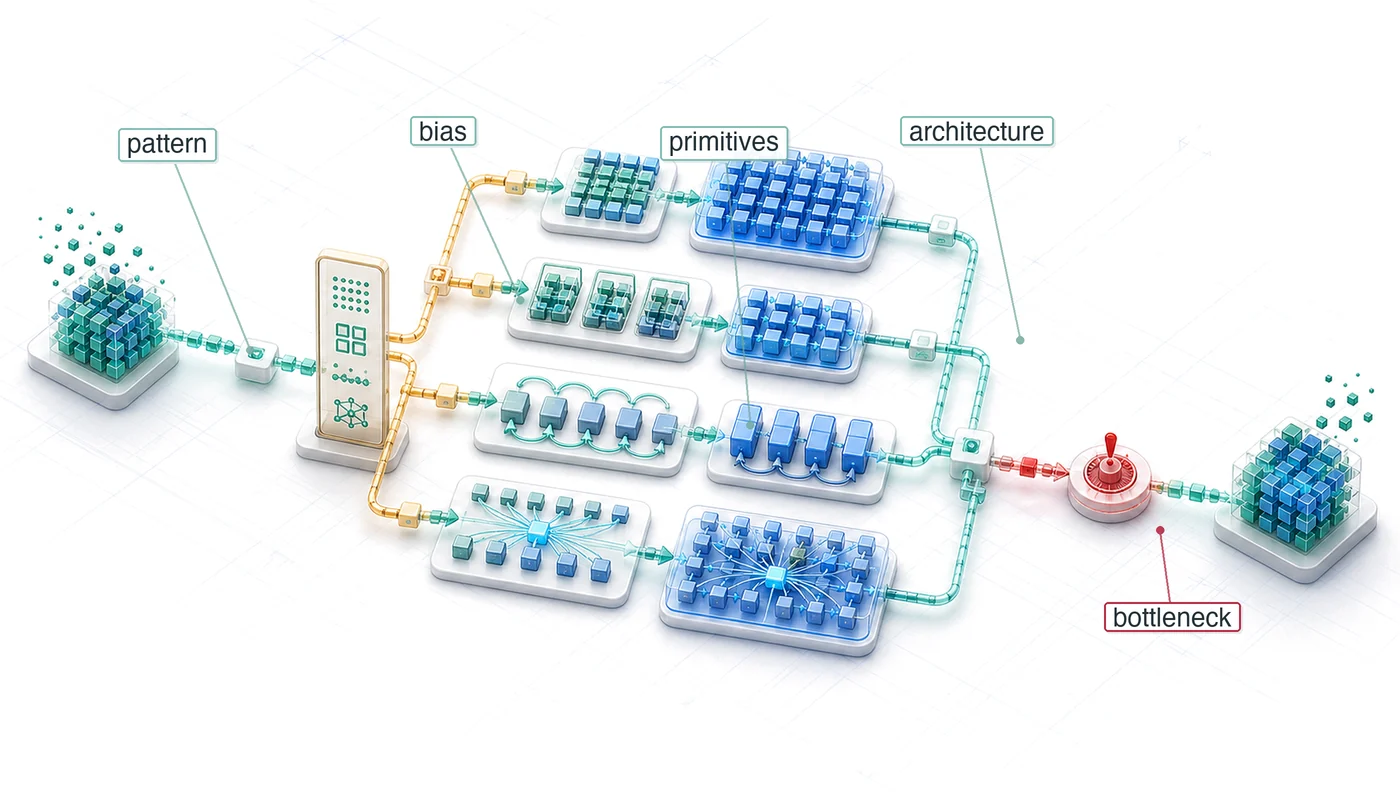
Selecting a neural network architecture is both a modeling decision and a contract with physics. The commitment begins with the structure in the data. An architecture that matches that structure can learn with fewer parameters and examples, while a poor match spends additional data and machine time compensating for the wrong computational pattern. Convolution, attention, recurrence, and embedding lookup do not merely encode different assumptions about data; they create different patterns of computation, state, and data movement. Those patterns determine whether work parallelizes cleanly, whether intermediate state fits in memory, and whether training and serving remain affordable at the required scale. Two architectures can deliver similar predictive quality yet impose different memory footprints and latency profiles while exposing different opportunities for later efficiency techniques. Benchmark accuracy alone therefore cannot reveal which design remains viable. Architectural commitments also propagate beyond the model. Data pipelines adopt particular input structures, training infrastructure is provisioned around the model’s compute profile, serving systems are tuned to its request path, and monitoring inherits its failure modes. Once those dependencies accumulate, replacing the architecture can mean rebuilding much of the surrounding system. An architecture decision is sound only when its predictive gains remain compatible with the full deployment context. In D·A·M terms, architecture is algorithm-machine co-design at its root, with the mathematical graph determining the work the machine must perform and the machine budget limiting which graphs remain practical.

Learning Objectives

Distinguish computational characteristics of MLPs, CNNs, RNNs, Transformers, and DLRM-style recommenders
Explain how inductive biases exploit structure in different data types
Analyze computational complexity and memory scaling across architectural families
Identify building blocks such as skip connections, normalization, and gating that enable deep training
Apply the architecture selection framework to match data characteristics with model designs
Evaluate how compute, memory access, and data movement determine hardware mapping efficiency
Critique architecture-selection fallacies under latency, bandwidth, and parallelization constraints

Architectural Principles

A dense model spends parameters and memory on relationships an image rarely needs. Convolutional neural networks (CNNs) encode locality; multilayer perceptrons (MLPs) do not. Matrix multiplication, activation functions, and gradient computation form the “verbs” of neural networks. Architectures assemble those verbs into computational graphs: specialized structures optimized for specific data types and computational constraints. Under the silicon contract (principle 4), every architecture makes an implicit agreement with hardware, trading computational patterns for efficiency on particular problem classes.

Inductive bias from strong (CNN) to weak (MLP): stronger prior, less data needed.

¹ Inductive bias: From Latin inducere, “to lead into,” encoding a structural assumption “leads” the model toward a smaller solution space, which is why this concept unifies the entire chapter: every architecture discussed here—multilayer perceptron (MLP), convolutional neural network (CNN), recurrent neural network (RNN), and transformer—is defined by its choice of bias. A CNN’s locality bias cuts parameters by orders of magnitude vs. an equivalent MLP, directly shrinking the iron law’s $O$ and $D_{\text{vol}}$ terms, while global attention trades quadratic score computation for long-range connectivity.

Every neural network architecture decides how computation should be organized to match the inherent structure in the data. Images have spatial locality, language has sequential dependencies, and tabular records often lack a fixed spatial or sequential organization. The architecture encodes assumptions about these patterns directly into the computational graph, and those assumptions influence parameter count, hardware utilization, and deployment feasibility. Architecture selection is therefore a systems engineering problem that directly affects the iron law terms: the number of operations $O$ and the volume of data movement $D_{\text{vol}}$. The structural assumptions that each architecture encodes are known as inductive biases,¹ and they serve as the unifying concept for this entire chapter.

Definition 1.1: Inductive bias

Inductive bias is a structural constraint built into a model architecture that restricts the hypothesis space, enabling generalization from finite data by encoding domain-specific assumptions (such as spatial locality or sequential ordering) directly into the computational graph.

Significance: Inductive bias can reduce the dataset size $(D)$ required for generalization. For one output feature detector, a dense connection uses $\mathcal{O}(N_{\text{pix}} C_{\text{in}})$ parameters, while a shared CNN filter uses $\mathcal{O}(K^2 C_{\text{in}})$ parameters and is applied at every position, costing $\mathcal{O}(N_{\text{pix}} K^2 C_{\text{in}})$ operations. For a $224{\times}224$ RGB image, a shared $3{\times}3$ filter therefore uses roughly 5,575.1× fewer parameters than one dense feature detector, reducing parameter storage and often the data required to avoid overfitting.
Distinction: Unlike regularization (which penalizes hypothesis complexity at training time via L1/L2 terms), inductive bias restricts the hypothesis space at architecture design time: a CNN represents nonlocal functions less directly than local patterns, while regularization discourages complexity through the training objective.
Common pitfall: A frequent misconception is that stronger inductive bias is always better. A strong locality bias (CNN) excels on spatial data but represents long-range dependencies in language less directly than global attention, which supports long-range dependencies at $\mathcal{O}(S^2)$ score-computation cost.

Architecture is the algorithm axis of D·A·M: it sets the operation-count budget.

A CNN encodes an inductive bias of spatial locality: nearby pixels matter more than distant ones. A transformer lets each element attend to any other, enabling long-range relationships at quadratic score-computation cost. These biases help architectures learn efficiently by restricting the space of functions they represent. Without an appropriate bias, a model may require substantially more data and compute to learn the same structure. The unified framework in section 1.10 brings these architectural families together once each bias has appeared in practice.

Machine learning systems face a core engineering trade-off: representational power vs. computational efficiency. Under the iron law of ML systems (principle 3), architectural choice is the primary determinant of the operation-count term $O$. A transformer’s attention mechanism enables global relationships but scales as $\mathcal{O}(S^2)$ operations with sequence length $S$; a CNN exploits spatial locality to reduce operations to linear scaling in the number of spatial positions. Matching the right inductive biases to a workload’s data while setting a manageable operation-count budget defines the practice of neural architecture selection.

Example 1.1: The ensemble Netflix did not ship (2009)

Context: Netflix awarded its $1M Grand Prize in 2009 for a 10 percent improvement in recommendation accuracy (Johnston 2012).

Mechanism: Bringing the winning improvement into production required substantial engineering effort just as Netflix’s business was shifting from mailed DVDs to streaming. That shift also produced richer viewing signals and changed what personalization needed to optimize.

Impact: The additional accuracy did not justify the production effort, so Netflix did not deploy the Grand Prize code.

Fix: Netflix retained two algorithms from the earlier Progress Prize and redirected its recommendation work toward streaming-era personalization.

Systems lesson: An offline metric gain is only valuable when its integration cost and objective still match the production system.

Johnston, Casey. 2012. “Netflix Never Used Its $1 Million Algorithm Due to Engineering Costs.” Ars Technica, April.

Choosing an architectural backbone sets the primary memory layout and compute pattern for downstream hardware. Table 1 contrasts the five major neural network families across their spatial/temporal inductive biases, tensor operations, and memory access characteristics.

Table 1: Neural Architecture Families: Each family targets a distinct data structure and exposes a distinct system bottleneck. The bottleneck column reads directly from the iron law: MLPs stress memory bandwidth through dense activations, CNNs stress compute throughput because convolution reuses filters across many pixels, RNNs stress sequential dependencies that prevent parallelism, transformers compute quadratic score interactions and may materialize quadratic score storage, and DLRM stresses memory capacity at terabyte scale through embedding tables.

Architecture	Data Type	Core Innovation	System Bottleneck
MLPs	Tabular/Unstructured	Dense connectivity	Memory bandwidth
CNNs	Spatial (images)	Local filters + weight sharing	Compute throughput
RNNs	Sequential (time series)	Recurrent state	Sequential dependencies
Transformers	Relational (language)	Dynamic attention	Quadratic score compute; optional $S^2$ storage
DLRM	Categorical (recommendations)	Embedding tables	Memory capacity (TB+)

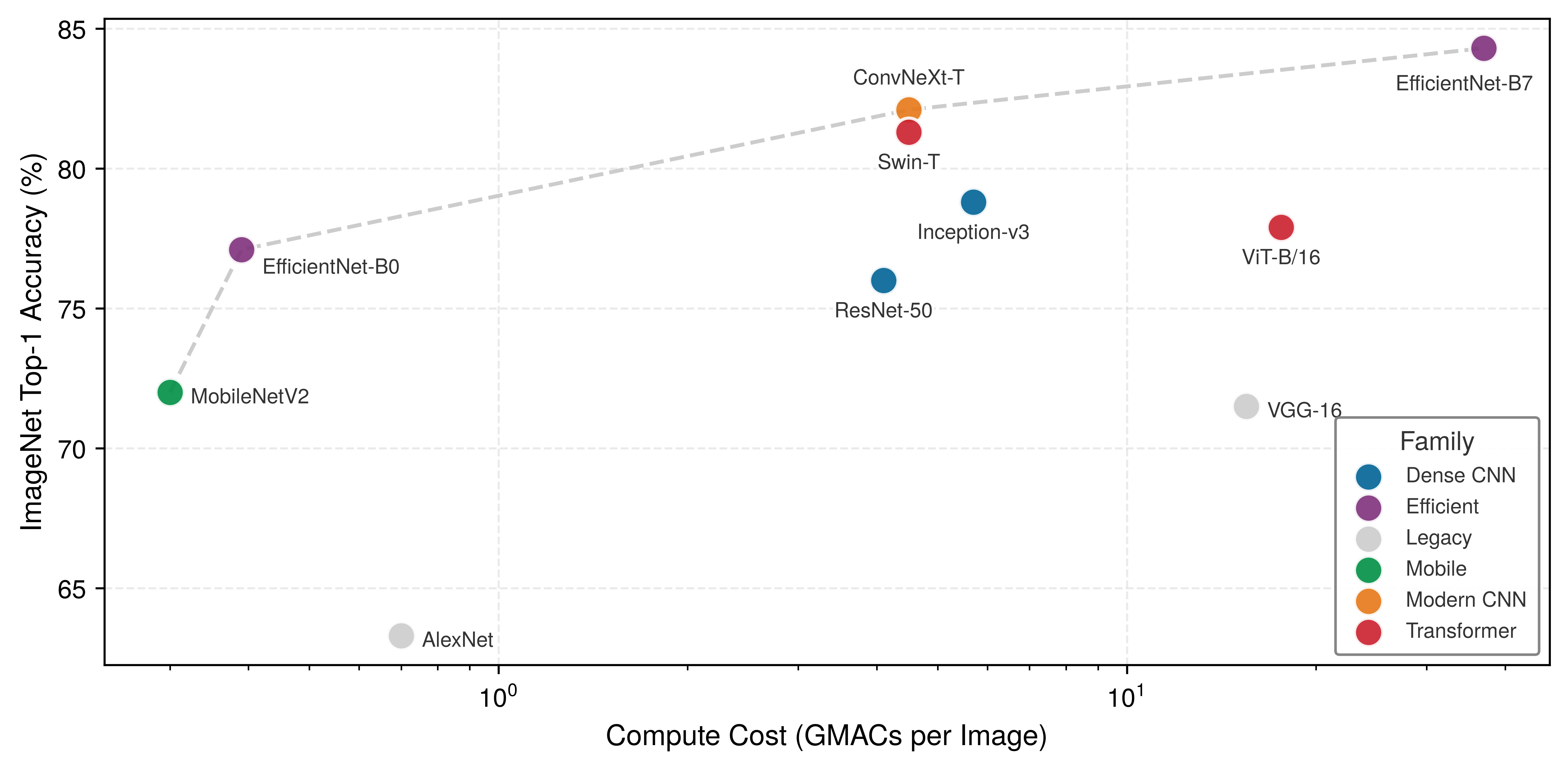
Five specific model architectures recur throughout this book as lighthouse models: consistent reference points that ground abstract concepts in concrete systems reality. These examples are concrete implementations of the Workload Archetypes (Compute Beast, Bandwidth Hog, etc.) introduced in Workload archetypes. To understand why these specific models were chosen, consider the history of model evolution through the lens of the Pareto frontier (figure 1).

Figure 1: **The Efficiency Frontier**: ImageNet Top-1 Accuracy vs. Computational Cost (GMACs). Representative points are compiled from published model reports for AlexNet, VGG, ResNet, Inception, MobileNetV2, EfficientNet, ViT, Swin Transformer, and ConvNeXt (Krizhevsky et al. 2012; Simonyan and Zisserman 2015; He et al. 2016a; Szegedy et al. 2015; Sandler et al. 2018; Tan and Le 2019; Dosovitskiy et al. 2021; Liu et al. 2021; Liu et al. 2022). The dashed ‘Pareto frontier’ is an illustrative trade-off curve rather than a benchmark rerun; exact accuracy and reported compute values vary by model variant, training recipe, implementation, and operation-counting convention (multiply-accumulates vs. floating-point operations). The legend distinguishes six families: legacy CNNs (gray), dense CNNs (blue), efficient Mobile architectures (green), EfficientNet-class models (violet), modern CNNs (orange), and Transformers (red). The frontier is led by the efficient and modern-CNN families; the Transformers trade substantial compute for flexible long-range modeling without dominating it, and ViT-B/16 sits below the frontier.

These models serve as canonical workloads for understanding system constraints. Each occupies a distinct position on the trade-off between accuracy and computational cost, as mapped in figure 1. The plotted frontier should be read as a historical map of representative architecture papers, not as a controlled benchmark table. It traces the progression from dense CNNs that prioritized accuracy, through MobileNets that reduced compute per unit of accuracy, to transformer architectures that trade substantial computational cost for flexible long-range modeling. Architectural choices made at design time determine where a system lands on this frontier.

Lighthouse roster: Model biographies

Five models earn the lighthouse role because each isolates one system bottleneck that recurs repeatedly: compute (ResNet-50), memory bandwidth (GPT-2), memory capacity (DLRM), edge latency (MobileNetV2), and always-on power for keyword spotting (KWS). The biographies that follow trace each model’s historical context and why it became a useful reference.

ResNet-50 (He et al. 2016a) anchors the compute-intensive vision lighthouse. The Residual Network (ResNet) addressed the degradation problem in very deep plain networks: adding layers could increase training error despite sufficient capacity. By introducing “skip connections” that improve optimization and gradient flow, it enabled networks of 50, 100, or even 1000 layers. The ResNet architecture won the ImageNet 2015 competition (with very deep 152-layer models), and ResNet-50 has become a widely used backbone and benchmark workload for computer vision. From a systems perspective, it is a highly regular, compute-intensive workload composed almost entirely of dense convolutions, making it a useful test for GPU floating-point throughput.

² Autoregressive generation: A decoding strategy where each output token is conditioned on all previously generated tokens, requiring a full model forward pass per token; for a 1.5B-parameter model in FP16, the weight-only batch-one model used here reads about 3 GB of weights per decoding step and yields a work-to-byte ratio of about 1 FLOP/byte. This low arithmetic intensity often makes batch-one and small-batch decoding bandwidth bound; larger batches can amortize weight traffic. During generation, serving systems also retain attention state from earlier tokens; section 1.5 names this state the key-value cache.

GPT-2 (Radford et al. 2019) anchors the bandwidth-bound language lighthouse. Generative Pre-trained Transformer 2 demonstrated that scaling up a simple decoder-only transformer architecture on massive datasets could produce coherent text generation. Unlike BERT, an encoder-style transformer that reads context in both directions, GPT-2 generates text sequentially (autoregressively²), creating substantial memory bandwidth pressure during batch-one and small-batch decoding because model weights are read for each decoding step. It serves as our archetype for large language models such as Llama and ChatGPT.

DLRM (Naumov et al. 2019) anchors the sparse-recommendation lighthouse. Meta open-sourced DLRM to expose a workload that differs from CNNs and transformers in a critical way. While vision and language models are compute-heavy, recommendation systems are memory-heavy. They must look up user and item preferences in massive embedding tables that can reach terabytes in size, creating unique challenges for latency-critical serving (Model Serving). DLRM is a useful benchmark for memory capacity and sparse memory access patterns in the data center.

Lighthouse 1.1: Canonical workloads

In computer architecture, the microprocessor without interlocked pipelined stages (MIPS) processor is often used to teach pipelining, not because it is the fastest available chip, but because it is the clearest embodiment of reduced instruction set computer (RISC) principles. Similarly, this book uses ResNet-50, GPT-2, DLRM, MobileNetV2, and KWS as canonical workloads. By studying these “lighthouses,” we learn engineering principles about math, memory movement, and locality that remain valid even as the specific “state of the art” model architectures evolve.

MobileNet (Howard et al. 2017) anchors the edge-efficiency lighthouse. MobileNet challenged the trend of ever-larger models by prioritizing efficiency. It popularized depthwise separable convolutions for efficient vision models, an architectural innovation that reduced FLOPs by 8–9$\times$ for $3{\times}3$ kernels with minimal accuracy loss. That smaller compute footprint made MobileNet a natural fit for compression and lower-precision deployment techniques [storing and computing with fewer bits per value] covered in Model Compression. It became a reference family for co-designing vision models with the battery and latency constraints of smartphones and embedded devices.

Warden, Pete. 2018. “Speech Commands: A Dataset for Limited-Vocabulary Speech Recognition.” arXiv Preprint arXiv:1804.03209, ahead of print. https://doi.org/10.48550/arXiv.1804.03209.

Warden, Pete, and Daniel Situnayake. 2020. TinyML: Machine Learning with TensorFlow Lite on Arduino and Ultra-Low-Power Microcontrollers. O’Reilly Media.

Banbury, Colby R, Chuteng Zhou, Igor Fedorov, Ramon Matas, Urmish Thakker, Dibakar Gope, Vijay Janapa Reddi, Matthew Mattina, and Paul N Whatmough. 2021. “MicroNets: Neural Network Architectures for Deploying TinyML Applications on Commodity Microcontrollers.” Proceedings of Machine Learning and Systems 3: 517–32.

Banbury, Colby, Vijay Janapa Reddi, Peter Torelli, Jeremy Holleman, Nat Jeffries, Csaba Kiraly, Pietro Montino, et al. 2021. “MLPerf Tiny Benchmark.” arXiv Preprint.

KWS (Warden 2018) anchors the always-on TinyML lighthouse. Keyword spotting models (like those detecting “Hey Siri” or “Ok Google”) represent the extreme end of efficiency. Designed to run on “always-on” microcontrollers with kilobyte-scale memory and milliwatt power budgets, these models (often depthwise separable CNNs) exemplify the constraints of TinyML (Warden and Situnayake 2020; C. R. Banbury et al. 2021; C. Banbury et al. 2021). They force engineers to count every byte and cycle, motivating extreme quantization (INT8 and INT4) and specialized hardware. Together, these biographies establish why the lighthouses are not a model catalog: each one isolates a different bottleneck signature that the arithmetic-intensity analysis can quantify.

Workload signatures: The arithmetic intensity spectrum

ResNet-50 reuses convolutional weights across many spatial positions, while batch-one GPT-2/Llama decode streams large weight and KV-cache state for one token at a time. That contrast motivates arithmetic intensity, the FLOP/byte ratio established in Neural Computation and used with a hardware roofline to assess whether a workload is likely to be compute or memory bound.

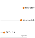
A weight-only proxy gives ResNet ~160$\times$ GPT-2’s batch-one intensity.

These bottlenecks reflect the underlying math, but the calculation here is a weight-only proxy rather than a complete measurement of main-memory traffic. It divides floating-point work by FP32 model-weight bytes, omitting activation, intermediate, and KV-cache traffic. Batching can amortize weight traffic across examples or tokens, while additional state movement can lower realized intensity. Computational complexity cheat sheet gives the per-operation FLOP and parameter formulas used in the proxy. Table 2 compares the three lighthouse scenarios and exposes a roughly 160.2× gap under these assumptions.

Table 2: Lighthouse Workload Signatures: Weight-only FP32 intensity proxies for three model scenarios. These values suggest different compute and bandwidth pressures but do not determine a fixed hardware affinity; realized bottlenecks depend on execution regime and hardware balance.

Model Family	Lighthouse	Intensity $(I)$	Hardware Affinity
Dense CNN	ResNet-50	~80.1 FLOP/byte	Compute-Rich (GPUs/TPUs)
Efficient Vision	MobileNetV2	~42.8 FLOP/byte	Balanced (Mobile NPUs)
Transformer	GPT-2 (Inf)	~0.50 FLOP/byte	Bandwidth-rich accelerator

This table provides one systems input to architecture selection. Task requirements determine which model families are viable, while batch size, precision, sequence length, implementation, cache behavior, and target hardware determine whether the proxy predicts the deployed bottleneck. MobileNet often suits constrained vision deployments, and batch-one transformer decoding often places heavy pressure on memory bandwidth, but both choices require measurement in the intended regime.

The “Bottleneck” column in table 3 deserves particular attention: it identifies which system resource (compute throughput, memory bandwidth, memory capacity, latency, or power) limits performance for each workload class. In iron law terms (Iron Law of ML Systems), the bottleneck identifies whether $O$ (operations) or $D_{\text{vol}}$ (data movement) dominates the runtime. These distinctions determine which optimization strategies prove effective throughout subsequent chapters.

Table 3: Lighthouse Model Comparison: Quantitative characteristics and pedagogical roles of the five canonical workloads. Memory is FP32 weight storage, and FLOPs are per inference except for GPT-2 XL, which is quoted per generated token; the DLRM row reports embedding-table entries rather than dense parameters. The bottleneck column indicates the primary system constraint each model reveals: compute-bound models like ResNet stress arithmetic throughput, while bandwidth-bound models like GPT-2 stress memory transfer rates.

Model	Domain	Params	FLOPs/Inf	Memory	Bottleneck	Role in Textbook
ResNet-50	Vision	25.6M	8.2 GFLOP	102.4 MB	Compute	Dense vision throughput
GPT-2 XL	Language	1.5B	3 GFLOP/token	6 GB	Mem. Bandwidth	Token-by-token serving
DLRM	Recommender	25B	Low	100 GB	Mem. Capacity	Embedding tables and capacity planning
MobileNetV2	Edge Vision	3.5M	600 MFLOP	14 MB	Latency	Depthwise convolutions and efficiency
KWS (DS-CNN)	Audio	200K	20 MFLOP	800 KB	Power	Always-on power budget

Architecture selection is ultimately an engineering trade-off between math $(O)$ and memory movement $(D_{\text{vol}})$. The mechanisms behind the signatures in table 2 explain why each lighthouse sits where it does on the intensity spectrum. ResNet-50 earns its high intensity because convolutional layers reuse each weight many times across the spatial dimensions of an image (deeper bottleneck layers reach 100–200+ FLOP/byte), so its performance is limited by how fast the hardware can do math. GPT-2 sits at the opposite extreme: each generated token produces only a matrix-vector multiplication rather than the matrix-matrix operations of batch processing, so the system loads massive weights from memory for a single token’s math, and performance is limited by how fast memory can move bits. MobileNet lands between the two at the whole-model level, with individual depthwise layers falling lower once activation traffic is included: depthwise separable convolutions reduce total $O$ but move more data relative to that work, which fits mobile hardware well yet often “starves” high-end GPUs optimized for dense math.

Checkpoint 1.1: Arithmetic intensity and architecture

Match the architectural choice to its systems implication:

Weight reuse (CNNs): how does reusing the same weights across many inputs change arithmetic intensity?
Large embedding tables (DLRM): how do massive embedding tables change the balance between data movement and computation?
Autoregressive decoding (GPT-2): why does token-by-token generation change the batching and bandwidth picture?

This spectrum determines whether the system needs a faster processor or faster memory to improve performance. The framework this book uses to quantify these limits on specific hardware is the roofline model, which plots achievable throughput against arithmetic intensity to show where a workload turns from memory bound to compute bound. The Roofline model gives the analytical treatment, with applied examples in Hardware Acceleration. A concrete example: The A100 analysis works this intensity-to-bottleneck classification through a real accelerator specification, computing the ridge point of an A100 and showing how the same operation falls on either side of it.

The lighthouse signatures make the next step concrete: inspect each architecture family by the data pattern it targets, the computation it performs, the hardware mapping it induces, and the bottleneck it exposes. This four-part lens ensures that every architecture is evaluated for what it costs to run, not only for what it learns.

Self-Check: Question

A team must choose between an MLP and a CNN for classifying $224 \times 224$ pixel RGB medical images. A single dense first layer would require $224 \times 224 \times 3 = 150{,}528$ input weights per output unit (yielding roughly 150 million weights for a 1,000-unit layer), whereas a CNN uses a shared $3 \times 3 \times 3$ filter (27 weights). Using the chapter’s framing of inductive bias, which statement best explains why the CNN is the superior starting point?
1. The CNN is strictly more expressive than the MLP, allowing it to approximate non-continuous functions that the Universal Approximation Theorem forbids.
2. The MLP is mathematically incapable of representing any 2D spatial feature mapping due to lack of convolutional instruction support.
3. The CNN eliminates gradient descent during optimization because convolutional spatial filters are deterministic, handcrafted operators.
4. The CNN’s spatial locality and weight-sharing prior directly matches the 2D structure of image data, collapsing parameter storage by over $5{,}000\times$ and drastically reducing sample complexity and memory traffic.
A dense MLP layer running batch-1 FP32 inference reports an arithmetic intensity of $\approx 0.5\text{ FLOP/byte}$, while an image convolution bottleneck layer achieves $>50\text{ FLOP/byte}$ on the same accelerator. Using the roofline model and an accelerator ridge point of $150\text{ FLOP/byte}$, explain why these kernels occupy opposite execution regimes and diagnose why upgrading to an accelerator with double the peak TFLOP/s will not speed up the batch-1 MLP.
Because an inductive bias restricts the hypothesis space to a smaller set of representable functions, machine learning systems engineers should always select the architecture with the strongest possible inductive bias for every workload.
A production profiler reveals that a model’s embedding tables consume over 1 TB of memory across cluster nodes, inference requests perform sparse random row lookups rather than dense matrix multiplies, and accelerator compute units remain over 95% idle. Which lighthouse archetype best represents this workload’s dominant system constraint?
1. DLRM, because the binding constraint is memory capacity for terabyte-scale embedding tables accessed via sparse, irregular memory gathers.
2. ResNet-50, because it stresses dense matrix floating-point throughput across regular convolutional grids.
3. GPT-2, because autoregressive decoding is the canonical memory-bandwidth-limited serving workload.
4. MobileNetV2, because depthwise-separable convolutions produce low arithmetic intensity on server GPUs.
Why does the chapter describe selecting a neural network architecture as ‘signing a contract with physics’ rather than merely selecting a mathematical modeling preference? Explain how architectural graph structure fixes terms in the iron law of ML systems ($T_{\text{exec}} = D_{\text{vol}}/\text{BW} + O/(R_{\text{peak}} \cdot \eta_{\text{hw}}) + L_{\text{lat}}$).

See Answers →

MLPs: Dense Pattern Processing

Consider a smartphone’s spam filter: given a set of features extracted from an email (sender reputation score, number of links, presence of certain keywords), the model must output a single probability: spam or not. This classification task, where every input feature connects to every output, is the domain of fully connected networks. MLPs³ represent the fully connected architectures introduced in Neural Computation, now examined through the four-part systems lens established earlier.

³ Perceptron: Formed from “perception” and the device suffix “-tron” (as in cyclotron and klystron), coined by Frank Rosenblatt (Rosenblatt 1957) for the atomic unit of neural computation: a weighted sum followed by a nonlinear activation, extending the earlier McCulloch-Pitts neuron. MLPs are composed entirely of these units arranged in fully-connected layers, so the efficiency of this single operation, a multiply-accumulate, determines system throughput. Modern accelerators execute over $10^{14}$ of these operations per second, making the perceptron the computational primitive that the entire ML hardware ecosystem is optimized around.

Rosenblatt, Frank. 1957. The Perceptron: A Perceiving and Recognizing Automaton. Report 85-460-1. Cornell Aeronautical Laboratory.

⁴ Universal approximation theorem (UAT): This theorem provides the mathematical guarantee for the MLP’s “no prior structure” inductive bias by proving a sufficiently wide network can approximate any continuous function. The systems-level catch is that “sufficiently wide” can require a number of neurons that grows exponentially with input dimensionality, rendering the theoretical guarantee practically unattainable for even moderately-sized inputs like a $256{\times}256$ image.

Cybenko, George. 1989. “Approximation by Superpositions of a Sigmoidal Function.” Mathematics of Control, Signals, and Systems 2 (4): 303–14. https://doi.org/10.1007/bf02551274.

Hornik, Kurt, Maxwell Stinchcombe, and Halbert White. 1989. “Multilayer Feedforward Networks Are Universal Approximators.” Neural Networks 2 (5): 359–66. https://doi.org/10.1016/0893-6080(89)90020-8.

MLPs embody an inductive bias: they assume no prior structure in the data, allowing any input to relate to any output. This architectural choice enables maximum flexibility by treating all input relationships as equally plausible, making MLPs versatile but computationally intensive compared to specialized alternatives. Their computational power was established theoretically by the Universal Approximation Theorem (UAT)⁴ (Cybenko 1989; Hornik et al. 1989), which we encountered as a footnote in Neural Computation. This theorem states that a sufficiently large MLP with nonlinear activation functions can approximate any continuous function on a compact domain, given suitable weights and biases. That combination of theoretical universality and dense connectivity is the architectural concept captured by the multilayer perceptron.

Definition 1.2: Multilayer perceptrons

Multilayer perceptrons are feed-forward neural network architectures that apply fully connected layers in sequence, where every neuron in one layer connects to every neuron in the next, encoding no structural assumption about the input domain.

Significance: The lack of structural prior gives dense layers quadratic parameter scaling in layer width: a single layer mapping 1,024 inputs to 1,024 outputs requires 1,048,576 parameters and about 2.1 MB of weight memory in FP16. A $3{\times}3$ convolution mapping 1,024 input channels to 1,024 output channels has about 9.4M weights; convolution’s advantage for images comes from spatial weight sharing across positions, not from reducing the channel-mixing matrix itself. This makes MLPs inefficient for high-dimensional structured inputs like images.
Distinction: Unlike convolutional neural networks, which exploit spatial locality to reduce parameter count, MLPs treat all input elements symmetrically, making them the architecture of choice for tabular data where no spatial or sequential structure is present.
Common pitfall: A frequent misconception is that MLPs are too simple to matter for complex tasks. MLPs provide a useful dense baseline, but CNNs, recurrent networks, and transformers add operators and connectivity patterns that cannot be reduced to weight sharing alone.

In practice, the UAT explains why MLPs succeed across diverse tasks while revealing the gap between theoretical capability and practical implementation. The theorem guarantees that some MLP can approximate any function, yet provides no guidance on requisite network size or weight determination. While MLPs can theoretically solve any pattern recognition problem, doing so may demand impractically large networks or prohibitive computation. This theoretical power drives the selection of MLPs for tabular data, recommendation systems, and problems where input relationships are unknown. At the same time, these practical limitations motivated the development of specialized architectures that exploit data structure for computational efficiency, as section 1.3, section 1.4, and section 1.6 demonstrate.

Learnability gap

The UAT sounds definitive, yet a fundamental gap separates what MLPs can represent from what they can learn in practice. That gap traces to a critical distinction between what a network can represent and what it can learn.

Representation capacity refers to the functions an architecture can express given unlimited resources; the UAT established earlier guarantees MLPs have universal representation capacity. This capacity is particularly effective because of the Manifold Hypothesis,⁵ which suggests that high-dimensional data actually occupies a much simpler structure. Learnability refers to whether gradient descent can find good weights given finite training samples and computational budgets. A function may be representable yet practically unlearnable.

⁵ Manifold hypothesis: The assumption that high-dimensional data lies on a low-dimensional surface embedded within the full space; a $256{\times}256$ image lives in a 65,536-dimensional space, but “valid cat images” occupy a tiny structured region. Deep networks progressively unfold this crumpled manifold into linearly separable representations. The systems consequence: if data truly occupied the full space, no architecture could learn from feasible dataset sizes; the manifold structure is what makes finite training budgets sufficient.

This distinction resolves the apparent paradox of universal approximation and architectural progress. Specialized architectures such as ResNets and transformers improve learnability by embedding inductive biases that match data structure, even when doing so restricts representational capacity.

Three factors create the learnability gap:

Sample complexity: The UAT provides no bounds on training examples needed. For $28{\times}28$ images, an MLP treats 784 pixels independently, requiring exponentially many samples to learn spatial correlations. A CNN embeds locality bias, drastically reducing sample requirements. Mathematically, sample complexity can scale exponentially with input dimension for MLPs but polynomially for architectures matching data structure.
Parameter efficiency: The UAT guarantees some width suffices, but provides no constructive bounds. Some function classes require widths that grow rapidly with input dimension, while architectures with a matching compositional structure can represent them more compactly.
Optimization difficulty: Even when optimal weights exist, gradient descent may not find them. MLP loss surfaces exhibit complex topology without the regularizing effect of architectural constraints. Specialized architectures reduce the search space, introducing symmetries that gradient descent exploits. The classic MNIST handwritten digit benchmark illustrates this gap between representation and learnability concretely.

Example 1.2: MNIST: Representation vs. learnability

Scenario: Classifying $28{\times}28$ MNIST digits using a fully connected MLP versus a CNN.

Diagnosis: A 3-layer MLP requires 20M parameters because it treats all 784 input pixels independently, ignoring spatial structure. A CNN uses local receptive fields and weight sharing, cutting parameters to 421.4K (47× fewer parameters).

Systems lesson: Inductive bias drives parameter efficiency. Incorporating spatial locality into model architecture reduces parameter footprint by orders of magnitude, lowering SRAM memory bandwidth pressure during inference.

The learnability gap motivates the core design principle of this chapter: embed inductive biases that match data structure. Each architecture sacrifices theoretical generality for practical learnability. The No Free Lunch theorem⁶ (Wolpert and Macready 1997) formalizes this trade-off: the bias that helps one task may hurt another. CNN’s translation invariance aids image classification but hurts tasks where absolute position matters. Architecture selection is fundamentally the act of matching inductive bias to data structure.

⁶ No free lunch theorem: Wolpert and Macready’s 1997 result proved that no optimization algorithm outperforms random search across all possible problems: averaged over every conceivable function, all algorithms are equivalent. The ML systems consequence is that an inductive bias (locality, equivariance, attention) can improve performance on problems matching that bias while hurting performance when its assumptions do not hold, making architecture selection an engineering commitment to a problem class.

Wolpert, D. H., and W. G. Macready. 1997. “No Free Lunch Theorems for Optimization.” IEEE Transactions on Evolutionary Computation 1 (1): 67–82. https://doi.org/10.1109/4235.585893.

These theoretical insights translate directly into engineering decisions. Appropriate inductive biases reduce parameter counts (enabling edge deployment), accelerate convergence (reducing training costs), and produce structured computation patterns that map efficiently to specialized hardware (Hardware Acceleration). A 20M-parameter MLP infeasible for edge deployment becomes a 421.4K-parameter CNN that fits comfortably, a 47× reduction achieved by matching architecture to data structure. The next question is what specific pattern processing requirements dense architectures address.

Pattern processing needs

Deep learning models frequently encounter problems where any input feature may influence any output without inherent constraints. In financial market analysis, any economic indicator may affect any market outcome. In natural language processing, word meaning may depend on any other word in the sentence. These scenarios demand an architectural pattern capable of learning arbitrary relationships across all input features. The architecture must provide unrestricted feature interactions where each output can depend on any combination of inputs, learned feature importance where the system determines which connections matter rather than relying on prescribed relationships, and adaptive representation where the network reshapes internal representations based on the data itself.

The MNIST digit recognition task illustrates this uncertainty concretely. While humans might focus on specific parts of digits (loops in ‘six’ or crossings in ‘eight’), the pixel combinations critical for classification remain indeterminate. A ‘seven’ written with a serif may share pixel patterns with a ‘two’, and variations in handwriting mean discriminative features may appear anywhere in the image. This uncertainty about feature relationships requires a dense processing approach where every pixel can potentially influence the classification decision—an architectural commitment that leads directly to the mathematical foundation of MLPs.

Algorithmic structure

These pattern processing needs demand an architecture capable of relating any input to any output. MLPs solve this with complete connectivity between all nodes. This connectivity requirement manifests through a series of fully-connected layers, where each neuron connects to every neuron in adjacent layers, the “dense” connectivity pattern introduced in Neural Computation.

Dense connectivity translates directly into fully connected layers and matrix multiplication operations, the mathematical basis introduced in Matrix multiplication formulation that makes MLPs computationally tractable. Figure 2 shows how each layer transforms its input through this core operation.

 \begin{tikzpicture}[line join=round,font=\sffamily]
\tikzset{%
Line/.style={line width=0.35pt,black!60}
}

\tikzset{
  box/.pic={
    \pgfkeys{/box/.cd, #1}
\foreach \x in {1,...,\columns}{
    \foreach \y in {1,...,\rows}{
        %
        \node[draw=black, fill=\ffill, minimum width=\cellsize,
                    minimum height=\cellheight, line width=\linewidth] (cell-\x-\y\br) at (\x*\cellsize,-\y*\cellheight) {};
    }
}
 } }

\pgfkeys{
  /box/.cd,
  cellsize/.store in=\cellsize,
  linewidth/.store in=\linewidth,
  cellheight/.store in=\cellheight,
  columns/.store in=\columns,
  br/.store in=\br,
  ffill/.store in=\ffill,
  rows/.store in=\rows,
  columns=1,
  rows=3,
  br=A,
  ffill=GreenL!22,
  cellsize=8mm,
  cellheight=8mm,
  linewidth=0.75pt
}
\def\radius{4mm}
\pic at (0,0) {box={columns=1,rows=4,br=A}};
\pic at (2,0) {box={columns=5,rows=4,br=B,}};
\pic at (7,4mm) {box={columns=1,rows=5,br=C}};
\pic at (9,4mm) {box={columns=2,rows=5,br=D}};
\pic at (12,-8mm) {box={columns=1,rows=2,br=E}};
%
\foreach \x in {1,...,4}{
\node[fill=green!80!black!80,minimum size=\cellsize,draw, line width=0.75pt]at(cell-2-\x B){};
}
\node[fill=green!80!black!80,minimum size=\cellsize,draw, line width=0.75pt]at(cell-1-2C){};

\begin{scope}[scale=1, every node/.append style={transform shape},
local bounding box=D1,shift={($(cell-1-3A)+(-4.5,-2.6)$)}]
\foreach \x in {1,...,5}{
\coordinate (2ball-\x) at (0,\x);
\shade[shading=ball,ball color=red!50!yellow] (0,\x) circle (\radius);
}
\shade[shading=ball,ball color=green!50!green] (0,4) circle (\radius);

\foreach \x/\i in {2.5/1,3.5/2}{
\coordinate (3ball-\i) at (2,\x);
\shade[shading=ball,ball color=red!50!yellow] (2,\x) circle (\radius)coordinate(3C\i);
}

\foreach \x/\i in  {1.5/1,2.5/2,3.5/3,4.5/4}{
\coordinate (1ball-\i) at (-2,\x);
\shade[shading=ball,ball color=red!50!yellow] (-2,\x) circle (\radius)coordinate(1C\i);
}
% Connect 1. and 2. column
\foreach \x in {1,2,3,4}{
  \foreach \y in {1,2,3,5}{
    \edef\from{1ball-\x}
    \edef\to{2ball-\y}
\path let
    \p1 = (\from),
    \p2 = (\to),
    \n1 = {atan2(\y2-\y1,\x2-\x1)}
  in
    coordinate (from) at ($ (\from) + (\n1:\radius) $)
    coordinate (to) at ($ (\to) + (\n1+180:\radius) $);
  \draw[Line] (from) -- (to);
  }
}
%red line
\foreach \x in {1,2,3,4}{
  \foreach \y in {4}{
    \edef\from{1ball-\x}
    \edef\to{2ball-\y}
\path let
    \p1 = (\from),
    \p2 = (\to),
    \n1 = {atan2(\y2-\y1,\x2-\x1)}
  in
    coordinate (from) at ($ (\from) + (\n1:\radius) $)
    coordinate (to) at ($ (\to) + (\n1+180:\radius) $);
  \draw[Line,red] (from) -- (to);
  }
}
% Connect 2. and 3. column
\foreach \x in {1,2,3,4,5}{
  \foreach \y in {1,2}{
    \edef\from{2ball-\x}
    \edef\to{3ball-\y}
\path let
    \p1 = (\from),
    \p2 = (\to),
    \n1 = {atan2(\y2-\y1,\x2-\x1)}
  in
    coordinate (from) at ($ (\from) + (\n1:\radius) $)
    coordinate (to) at ($ (\to) + (\n1+180:\radius) $);
  \draw[Line] (from) -- node[inner sep=0pt](L\x){}(to);
  }
}
%%
\draw[latex-](L5)--++(30:1)node[above]{Weighted Edge};
\draw[latex-](2ball-4)--++(180:2.5)node[left](NE){Neuron};
\draw[thick,latex-](cell-2-2B.center)--++(90:1.52)node[above]{Weighted Edge};
\draw[thick,latex-](cell-1-2C.center)--++(90:1.52)node[above]{Neuron};
%
\node[font=\huge]at($(cell-1-2A.south east)!0.5!(cell-1-2B.south west)$){$\times$};
\node[font=\huge]at($(cell-1-3C.east)!0.5!(cell-1-3D.west)$){$\times$};
%
\node[single arrow, draw=red, fill=red,
      minimum width = 10pt, single arrow head extend=3pt,
      minimum height=7mm]at($(cell-5-2B.south east)!0.5!(cell-1-3C.west)$){};
\node[single arrow, draw=red, fill=red,
      minimum width = 10pt, single arrow head extend=3pt,
      minimum height=7mm]at($(cell-2-3D.east)!0.5!(cell-1-1E.south west)$){};
\end{scope}

\path(NE.west)--++(270:4.0)coordinate(IL1)-|coordinate(HL1)($(1ball-1)!0.4!(2ball-1)$);
\path(NE)--++(270:4.0)-|coordinate(OL1)($(2ball-1)!0.55!(3ball-1)$);
\path(NE)--++(270:4.0)-|coordinate(OL2)($(3ball-1)!0.5!(cell-1-2A.south east)$);
\path(NE)--++(270:4.0)-|coordinate(IL2)($(3ball-1)!0.6!(cell-1-2A.south east)$);

\path[blue, line width=2pt](IL2)-|coordinate(HL2)($(cell-1-2A.south east)!0.7!(cell-1-2B.south west)$);
\path[blue, line width=2pt](IL2)-|coordinate(OL3)($(cell-1-3C.east)!0.5!(cell-1-3D.west)$);
\path[blue, line width=2pt](IL2)-|coordinate(OL4)(cell-1-2E.south east);

\draw[red,line width=2pt](IL1)--node[below,text=black]{Input Layer}(HL1);
\draw[cyan,line width=2pt](HL1)--node[below,text=black]{Hidden Layer}(OL1);
\draw[brown,line width=2pt](OL1)--node[below,text=black]{Output Layer}(OL2);
%
\draw[red,line width=2pt](IL2)--node[below,text=black]{Input Layer}(HL2);
\draw[cyan,line width=2pt](HL2)--node[below,text=black]{Hidden Layer}(OL3);
\draw[brown,line width=2pt](OL3)--node[below,text=black]{Output Layer}(OL4);
\end{tikzpicture}

Figure 2: Multilayer Perceptron Architecture: A three-layer network in which every neuron connects to all neurons in adjacent layers. The highlighted neuron receives weighted contributions from all inputs, illustrating the dense $\mathcal{O}(N \times M)$ connectivity pattern implemented through matrix multiplications. For MNIST classification, a 784-dimensional input connects to 100 hidden neurons through a $784{\times}100$ weight matrix, requiring 78,400 multiply-accumulate operations per sample. Adapted from (Reagen et al. 2017).

Reagen, Brandon, Robert Adolf, Paul Whatmough, Gu-Yeon Wei, and David Brooks. 2017. Deep Learning for Computer Architects. Synthesis Lectures on Computer Architecture. Springer International Publishing. https://doi.org/10.1007/978-3-031-01756-8.

Equation 1 expresses the dense layer’s affine transformation followed by its activation. \[ \mathbf{h}^{(\ell)} = f\big(\mathbf{h}^{(\ell-1)}\mathbf{W}^{(\ell)} + \mathbf{b}^{(\ell)}\big) \tag{1}\]

$\mathbf{h}^{(\ell)}$ represents the layer $\ell$ output, $\mathbf{h}^{(\ell-1)}$ represents the input from the previous layer, $\mathbf{W}^{(\ell)}$ denotes the weight matrix for layer $\ell$, $\mathbf{b}^{(\ell)}$ denotes the bias vector, and $f(\cdot)$ denotes the activation function; Nonlinear activation functions develops the rectified linear unit (ReLU) and related nonlinearities in detail. This layer-wise transformation, while conceptually simple, creates computational patterns whose efficiency depends critically on how we organize these operations for different problem structures.

The dimensions of these operations reveal the computational scale of dense pattern processing. The input vector $\mathbf{h}^{(0)} \in \mathbb{R}^{d_{\text{in}}}$ (treated as a row vector in this formulation) represents all potential input features. Weight matrices $\mathbf{W}^{(\ell)} \in \mathbb{R}^{d_{\text{in}} \times d_{\text{out}}}$ capture all possible input-output relationships. The output vector $\mathbf{h}^{(\ell)} \in \mathbb{R}^{d_{\text{out}}}$ produces transformed representations. A four-pixel example turns this bookkeeping into arithmetic.

Example 1.3: Concrete computation example

Consider a simplified 4-pixel image processed by a 3-neuron hidden layer:

Input: $\mathbf{h}^{(0)} = [0.8, 0.2, 0.9, 0.1]$ (4 pixel intensities)

Weight matrix: \[ \mathbf{W}^{(1)} = \begin{bmatrix} 0.5 & 0.1 & -0.2 \\ -0.3 & 0.8 & 0.4 \\ 0.2 & -0.4 & 0.6 \\ 0.7 & 0.3 & -0.1 \end{bmatrix}\quad (4{\times}3 \text{ matrix}) \]

Computation: \[\begin{gather*} \mathbf{z}^{(1)} = \mathbf{h}^{(0)}\mathbf{W}^{(1)} = \begin{bmatrix} 0.5{\times}0.8 + (-0.3)\times 0.2 + 0.2{\times}0.9 + 0.7{\times}0.1 \\ 0.1{\times}0.8 + 0.8{\times}0.2 + (-0.4)\times 0.9 + 0.3{\times}0.1 \\ (-0.2)\times 0.8 + 0.4{\times}0.2 + 0.6{\times}0.9 + (-0.1)\times 0.1 \end{bmatrix} = \begin{bmatrix} 0.59 \\ -0.09 \\ 0.45 \end{bmatrix} \end{gather*}\] After ReLU: $\mathbf{h}^{(1)} = [0.59, 0, 0.45]$ (negative values zeroed)

Systems insight: Each hidden neuron combines all input pixels with different weights, demonstrating unrestricted feature interaction. Dense layers buy generality by paying the maximum connectivity cost.

The MNIST example makes this scale concrete. The 784-dimensional input connects to every neuron in the first hidden layer. A hidden layer with 100 neurons requires a $784{\times}100$ weight matrix (78,400 parameters), where each weight represents a learnable relationship between an input pixel and a hidden feature. This single layer anchors the computational analysis throughout this chapter.

This algorithmic structure enables arbitrary feature relationships while creating specific computational patterns that computer systems must accommodate. Dense connectivity provides the universal approximation capability established earlier but introduces computational redundancy: while the theoretical power of MLPs enables modeling of any continuous function given sufficient width, this flexibility requires numerous parameters to learn relatively simple patterns. Every input feature influences every output, yielding maximum expressiveness at the cost of maximum computational expense. These trade-offs motivate later compression strategies that reduce computational demands while preserving model capability, and Hardware Acceleration explores hardware-specific implementations that exploit regular matrix operation structure.

Computational mapping

Section 1.2.3 defines what an MLP computes; computational mapping reveals how that computation translates to hardware operations. Listing 1 demonstrates how this mapping progresses from mathematical abstraction to computational reality.

Listing 1: MLP Layer in Matrix Form: Framework-level matrix operations hide $\mathcal{O}(B \times d_{\text{in}} \times d_{\text{out}})$ multiply-accumulate complexity behind a single function call, enabling hardware-optimized BLAS libraries to use dense matrix hardware efficiently.

def mlp_layer_matrix(X, W, b):
    """MLP forward pass using framework-level matrix operations."""
    # X: input matrix (batch_size by num_inputs)
    # W: weight matrix (num_inputs by num_outputs)
    # b: bias vector (num_outputs)

    # Single GEMM call: frameworks dispatch to optimized BLAS/cuBLAS
    # For MNIST: 784 * 100 = 78,400 MACs per sample
    H = activation(matmul(X, W) + b)
    return H

The function mlp_layer_matrix directly mirrors the mathematical equation, employing high-level matrix operations (matmul) to express the computation in a single line while abstracting the underlying complexity. This implementation style characterizes deep learning frameworks, where optimized libraries manage the actual computation.

To understand the system implications of this architecture, we must look “under the hood” of the high-level framework call. The elegant one-line matrix multiplication output = matmul(X, W) is, from the hardware’s perspective, a series of nested loops that expose the true computational demands on the system. This translation from logical model to physical execution reveals critical patterns that determine memory access, parallelization strategies, and hardware utilization.

The second implementation in listing 2 exposes the actual computational pattern through nested loops, revealing what really happens when we compute a layer’s output: we process each sample in the batch, computing each output neuron by accumulating weighted contributions from all inputs. This translation from mathematical abstraction to concrete computation exposes how dense matrix multiplication decomposes into nested loops of simpler operations. The outer loop processes each sample in the batch, while the middle loop computes values for each output neuron. Within the innermost loop, the system performs repeated multiply-accumulate operations,⁷ combining each input with its corresponding weight.

⁷ MAC (multiply-accumulate): The atomic operation of neural networks: multiply two values and add to a running sum. In Horowitz’s 45 nm reference, an FP32 multiply plus add costs about 4.6 pJ, while a 32-bit off-chip DRAM access costs about 640 pJ (Horowitz 2014). These technology-specific values illustrate why data movement can dominate arithmetic energy; they are not universal constants for current hardware.

Horowitz, Mark. 2014. “1.1 Computing’s Energy Problem (and What We Can Do about It).” 2014 IEEE International Solid-State Circuits Conference Digest of Technical Papers (ISSCC), 10–14. https://doi.org/10.1109/isscc.2014.6757323.

Listing 2: Dense Layer Computation: Nested loops reveal $\mathcal{O}(B \times d_{\text{out}} \times d_{\text{in}})$ complexity where each output neuron requires num_inputs multiply-accumulate operations, so the reference MNIST input layer requires 78,400 MACs per sample.

def mlp_layer_compute(X, W, b):
    """Explicit loop structure exposing MLP computational patterns."""
    # Loop 1: Process each sample independently (parallelizable)
    for batch in range(batch_size):
        # Loop 2: Compute each output neuron
        for out in range(num_outputs):
            Z[batch, out] = b[out]  # Initialize with bias

            # Loop 3: Accumulate weighted inputs (innermost loop)
            # This is the MAC operation: result += input * weight
            for in_ in range(num_inputs):
                Z[batch, out] += X[batch, in_] * W[in_, out]
            # Total per output: num_inputs MACs +
            # num_inputs memory reads

    H = activation(Z)  # Element-wise nonlinearity
    return H

In our reference MNIST layer, each output neuron requires 78,400 MACs divided by 100, or 784, multiply-accumulate operations and at least 1,568 memory accesses (784 for inputs, 784 for weights). Production implementations call optimized matrix libraries such as Basic Linear Algebra Subprograms (BLAS),⁸ but the same nested-loop pattern still determines the system design problem. The hardware architectures that accelerate these matrix operations, including GPU Tensor Cores⁹ and specialized AI accelerators, are covered in Hardware Acceleration.

⁸ BLAS (basic linear algebra subprograms): This standard API for matrix operations enables the use of highly optimized libraries (for example, cuBLAS) to accelerate the 784 multiply-accumulates per neuron. The $784{\times}100$ matrix in the MNIST example may use the hardware less efficiently than larger, well-aligned transformer matrices because utilization depends on matrix shape, batching, datatype, library, and accelerator.

⁹ Tensor Cores: Specialized units in NVIDIA GPUs that accelerate the thousands of multiply-accumulate operations described by fusing them into single, highly parallelized matrix instructions. Tensor Cores are most efficient when matrix dimensions meet datatype- and architecture-specific alignment multiples; modern cuBLAS/cuDNN can still use Tensor Cores for many nonaligned cases, often with lower efficiency or internal padding. The architectural lesson is vendor-independent: specialized matrix units reward dense, aligned general matrix multiplication (GEMM) workloads and penalize small, irregular shapes that cannot keep the units full.

System implications

Section 1.2.4 showed how MLP operations decompose into nested loops of multiply-accumulate operations. The system-level constraints that emerge from these patterns span three dimensions: memory requirements, computation needs, and data movement.

For dense pattern processing, the memory, compute, and data-movement costs all come from the same source: all-to-all connectivity. Memory usage is dominated by parameter storage. Our reference MNIST layer $(784{\times}100)$ requires only 78,400 parameters, but this $\mathcal{O}(M \times N)$ scaling becomes prohibitive for high-dimensional inputs. A typical 2048-unit layer connected to a 2048-unit layer requires 4,194,304 parameters (16.8 MB at FP32). Since every weight is used exactly once per input vector, there is no opportunity for weight reuse within a single sample processing, making the workload heavily dependent on memory capacity and bandwidth.

The core computation is dense GEMV, or GEMM when batched. This computation is regular and parallelizable, but the arithmetic intensity (FLOP/byte) is low for small batches. The batch size is the number of input samples processed together; larger batches amortize weight-loading cost over more computations. Modern processors optimize dense layers with single instruction, multiple data (SIMD) units such as AVX-512 on CPUs or systolic arrays on Tensor Processing Units (TPUs) and GPUs, amortizing control overhead over large blocks of parallel arithmetic.

The resulting bottleneck is data movement. To compute 100 hidden values from 784 inputs, the system must move $784{\times}100$ weights from memory to the compute units. Applying the arithmetic intensity framework from section 1.1.2 to this layer yields roughly 0.5 FLOP/byte for batch-one FP32 execution. Under a weight-only model that counts one FP32 read per weight and omits input, output, bias, and cache traffic, equation 2 gives this ratio, where $M$ and $N$ are the input and output widths. \[ \text{Intensity} \approx \frac{2 \cdot M \cdot N \text{ FLOPs}}{4 \cdot M \cdot N \text{ bytes}} = 0.5 \text{ FLOP/byte} \tag{2}\]

On accelerators with ridge points in the hundreds of FLOP/byte, this batch-one FP32 layer is memory-bandwidth bound. Batching can raise intensity by amortizing weight traffic, but the crossover depends on matrix shape, precision, implementation, and hardware. This is why fully connected layers can become inference bottlenecks despite performing fewer total FLOPs than convolutional layers.

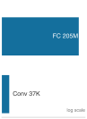
Weight sharing spares convolution the fully-connected parameter explosion.

Dense connectivity thus moves maximum data for minimum compute. For data with inherent structure (such as spatial locality in images or temporal order in sequences), specialized architectures can exploit that structure for both better accuracy and better efficiency. The most established such architecture is the convolutional neural network.

Self-Check: Question

A fully connected layer connecting 2,048 input units to 2,048 output units stores approximately 4.19 million weights (~16.8 MB in FP32). When applied to high-resolution image inputs, dense layers suffer severe parameter explosion. Which statement best captures the systems mechanism behind the MLP’s parameter and memory scaling?
1. Dense layers use non-linear activations whose element-wise memory footprints dwarf the weight tensors by several orders of magnitude.
2. MLP bias vectors grow quadratically with the output dimension, dominating total layer memory storage.
3. The MLP encodes no structural prior about the input, requiring every input-output pair to maintain an independent learnable parameter, yielding $\mathcal{O}(M \times N)$ parameter storage and weight memory traffic per sample.
4. Dense layers require storing three master copies of every weight matrix in hardware registers during inference forward passes.
A team cites the Universal Approximation Theorem (UAT) to argue that a wide 3-layer MLP should be used to classify $256 \times 256$ RGB images instead of a CNN. Explain why UAT does not justify this design choice in practice, detailing both the statistical failure mode (sample complexity) and the systems failure mode (memory bandwidth and parameter explosion).
The ____ hypothesis states that high-dimensional real-world data (such as natural images) actually resides on a much lower-dimensional structured surface embedded within the full input space, explaining why deep neural networks can generalize from feasible training budgets despite the curse of dimensionality.
A single dense layer ($2{,}048 \times 2{,}048$) running FP32 inference on an A100 GPU at batch size 1 achieves only ~4% of peak compute throughput, with profilers reporting an arithmetic intensity of $\approx 0.5\text{ FLOP/byte}$. What is the most effective engineering solution to move this kernel out of the memory-bandwidth-bound regime and raise hardware utilization?
1. Increase the batch size ($B > 1$), transforming the matrix-vector multiplication (GEMV) into a matrix-matrix multiplication (GEMM), which amortizes weight loading across $B$ samples and scales arithmetic intensity.
2. Replace the dense matrix multiplication with an unvectorized scalar loop to avoid GPU kernel launch overhead.
3. Upgrade to an accelerator with double the peak FP32 TFLOP/s while keeping the batch size at 1.
4. Replace the linear transformation with an element-wise activation function to eliminate all weight memory traffic.
In the nested loop implementation of an MLP forward pass (for batch, for out, for in_), calculate the exact number of multiply-accumulate (MAC) operations and memory accesses required to compute 100 hidden neurons from a 784-dimensional MNIST input vector at batch size 1, and explain how framework-level BLAS libraries optimize this pattern.

See Answers →

CNNs: Spatial Pattern Processing

The MLP’s assumption that every input may interact directly with every output proves particularly costly for spatially structured data like images. As the earlier MNIST comparison demonstrated, the example CNN uses 47× fewer parameters by exploiting spatial locality rather than treating every pixel independently.

Convolutional neural networks (CNNs)¹⁰ emerged as the solution to this challenge (LeCun et al. 1998; Krizhevsky et al. 2012). Consider what happens when viewing a photograph: the visual system does not perceive every pixel simultaneously in relation to every other pixel. Instead, it detects local patterns (edges, textures, corners) and composes them into objects. CNNs encode this same insight architecturally.

¹⁰ Convolution: From Latin convolvere (“to roll together”), describing a filter that slides across an input, combining local elements at each position. This “rolling together” enforces a locality constraint that is the source of the operation’s efficiency: a single $5{\times}5$ kernel reuses its 25 weights at every spatial position, reducing one feature detector for a 1-megapixel single-channel image from roughly 1,000,000 weights to 25, about 40,000$\times$ fewer parameters than a fully connected detector.

Spatial locality produces two key innovations that enhance efficiency for spatially structured data. Parameter sharing allows the same feature detector to be applied across different spatial positions, reducing parameters from millions to thousands while improving generalization. Local connectivity restricts connections to spatially adjacent regions, reflecting the insight that spatial proximity correlates with feature relevance. Together, these innovations define convolutional neural networks as an architectural family.

Definition 1.3: Convolutional neural networks

Convolutional neural networks (CNNs) are architectures that exploit translation equivariance and spatial locality to share learned filters across all spatial positions, decoupling parameter count from input resolution.

Significance: Weight sharing produces dramatic parameter reduction. A $3{\times}3$ convolutional layer with 64 input and 64 output channels requires $3 \times 3 \times 64 \times 64 \approx 37{,}000$ parameters regardless of whether the input image is $224{\times}224$ or $1024{\times}1024$. An equivalent fully connected layer on a $224{\times}224{\times}64$ input would require $224^2 \times 64 \times 64 \approx 205$ million parameters, a roughly 5,575$\times$ difference. This constant-parameter scaling enables CNNs to process high-resolution inputs within the memory budget of a single accelerator.
Distinction: Unlike MLPs, which connect every input element to every output element (global connectivity), CNNs restrict each output to a local spatial neighborhood, encoding the assumption that nearby pixels are more relevant than distant ones. This restriction eliminates entire hypothesis classes at architecture design time rather than penalizing them during training.
Common pitfall: A frequent misconception is that CNNs are vision-only models. The convolution operation applies to any data with a grid-like topology: 1D convolutions process audio waveforms and time series, 2D convolutions process images and spectrograms, and 3D convolutions process video and volumetric data.

The trade-off is explicit: CNNs sacrifice the theoretical generality of MLPs for practical efficiency gains when data exhibits known structure. Where MLPs treat each input element independently, CNNs exploit spatial relationships to achieve both computational savings and improved accuracy on vision tasks.

Pattern processing needs

Spatial pattern processing addresses scenarios where the relationship between data points depends on their relative positions or proximity. Consider processing a natural image: a pixel’s relationship with its neighbors is important for detecting edges, textures, and shapes. These local patterns then combine hierarchically to form more complex features: edges form shapes, shapes form objects, and objects form scenes. The pipeline in figure 3 gives this hierarchy a concrete visual form.

\begin{tikzpicture}[line join=round,font=\sffamily]
\tikzset{
 Line/.style={line width=0.5pt,black!50,text=black},
 LineD/.style={line width=0.5pt,black!50,text=black,dashed},
}

\tikzset{
channel/.pic={
\pgfkeys{/channel/.cd, #1}
\begin{scope}[yscale=\scalefac,xscale=\scalefac,every node/.append style={scale=\scalefac}]
\node[rectangle,draw=\channelcolor,line width=1pt,fill=\channelcolor!10,
minimum width=46,minimum height=56](\picname){};
\end{scope}
        }
}

\pgfkeys{
  /channel/.cd,
  channelcolor/.store in=\channelcolor,
  scalefac/.store in=\scalefac,
  picname/.store in=\picname,
  channelcolor=BrownLine,
  scalefac=1,
  picname=C
}
%circles sty
\tikzset{
circles/.pic={
\pgfkeys{/channel/.cd, #1}
\node[circle,draw=\channelcolor,line width=1pt,fill=\channelcolor!10,
minimum size=6mm](\picname){};
        }
}
%Zebra sty
\tikzset{
zebra/.pic={
\pgfkeys{/zebra/.cd, #1}
\definecolor{cfefefe}{RGB}{254,254,254}
\definecolor{c373435}{RGB}{55,52,53}
\begin{scope}[yscale=\globalscale,xscale=\globalscale,every node/.append style={scale=\globalscale}]
\path[fill=c373435,shift={(9.6358, -1.7033)}] (0.0, 31.4325).. controls (0.0427, 31.4009) and (0.0852, 31.369) .. (0.1273, 31.3366).. controls (0.1423, 31.3254) and (0.1573, 31.3141) .. (0.1728, 31.3026).. controls (0.2651, 31.2301) and (0.3393, 31.1462) .. (0.4151, 31.0574).. controls (0.4863, 30.9754) and (0.5596, 30.8955) .. (0.6333, 30.8157).. controls (0.6467, 30.8012) and (0.66, 30.7868) .. (0.6737, 30.7719).. controls (0.7542, 30.6847) and (0.8368, 30.6) .. (0.9211, 30.5164).. controls (0.9461, 30.4904) and (0.9461, 30.4904) .. (0.9717, 30.4639).. controls (0.9867, 30.4485) and (1.0016, 30.433) .. (1.017, 30.4172).. controls (1.0321, 30.4015) and (1.0471, 30.3858) .. (1.0627, 30.3696).. controls (1.1076, 30.325) and (1.1076, 30.325) .. (1.1857, 30.3047).. controls (1.1773, 30.338) and (1.169, 30.3713) .. (1.1604, 30.4056).. controls (1.0895, 30.6895) and (1.0185, 30.9733) .. (0.9475, 31.2572).. controls (0.9423, 31.2765) and (0.9371, 31.2958) .. (0.9317, 31.3157).. controls (0.9141, 31.3941) and (0.9166, 31.4684) .. (0.9211, 31.5483).. controls (0.9924, 31.6196) and (1.0315, 31.6099) .. (1.1311, 31.6111).. controls (1.5189, 31.6038) and (1.7672, 31.4046) .. (2.0276, 31.1361).. controls (2.5302, 30.5776) and (2.7987, 29.8516) .. (2.9904, 29.1373).. controls (3.0848, 28.7935) and (3.1926, 28.4518) .. (3.3106, 28.1153).. controls (3.3197, 28.0891) and (3.3197, 28.0891) .. (3.329, 28.0624).. controls (3.3457, 28.0158) and (3.3637, 27.9696) .. (3.3817, 27.9235).. controls (3.3965, 27.8817) and (3.3965, 27.8817) .. (3.4117, 27.839).. controls (3.4831, 27.7316) and (3.5705, 27.7011) .. (3.6876, 27.6539).. controls (3.7178, 27.6408) and (3.7178, 27.6408) .. (3.7487, 27.6275).. controls (3.8966, 27.5649) and (4.0474, 27.5172) .. (4.2019, 27.4737).. controls (4.1102, 27.846) and (4.0172, 28.2179) .. (3.9175, 28.5882).. controls (3.91, 28.6159) and (3.9026, 28.6436) .. (3.8949, 28.6721).. controls (3.8319, 28.9046) and (3.7693, 29.1311) .. (3.6727, 29.3522).. controls (3.6329, 29.4621) and (3.596, 29.5729) .. (3.5588, 29.6837).. controls (3.5098, 29.8269) and (3.4523, 29.9591) .. (3.3817, 30.093).. controls (3.333, 30.0443) and (3.3518, 29.9759) .. (3.3516, 29.911).. controls (3.3516, 29.8892) and (3.3517, 29.8673) .. (3.3517, 29.8448).. controls (3.3517, 29.8224) and (3.3517, 29.7999) .. (3.3517, 29.7768).. controls (3.3516, 29.7292) and (3.3517, 29.6815) .. (3.3518, 29.6339).. controls (3.3519, 29.5614) and (3.3518, 29.489) .. (3.3516, 29.4165).. controls (3.3516, 29.3702) and (3.3517, 29.3239) .. (3.3517, 29.2776).. controls (3.3517, 29.2453) and (3.3517, 29.2453) .. (3.3516, 29.2123).. controls (3.3521, 29.0889) and (3.362, 28.9717) .. (3.3817, 28.8495).. controls (3.3833, 28.806) and (3.384, 28.7624) .. (3.3834, 28.7189).. controls (3.3831, 28.6984) and (3.3829, 28.678) .. (3.3826, 28.657).. controls (3.3822, 28.6344) and (3.3822, 28.6344) .. (3.3817, 28.6114).. controls (3.2533, 28.7619) and (3.185, 28.9226) .. (3.1237, 29.1091).. controls (3.117, 29.1295) and (3.1103, 29.1498) .. (3.1034, 29.1708).. controls (2.925, 29.7222) and (2.7421, 30.3033) .. (2.7202, 30.8868).. controls (2.7192, 30.9105) and (2.7181, 30.9341) .. (2.717, 30.9585).. controls (2.7124, 31.1535) and (2.7119, 31.3674) .. (2.815, 31.5382).. controls (2.8862, 31.6082) and (2.9232, 31.6166) .. (3.0215, 31.6176).. controls (3.0495, 31.6169) and (3.0495, 31.6169) .. (3.078, 31.6162).. controls (3.1079, 31.6162) and (3.1079, 31.6162) .. (3.1383, 31.6162).. controls (3.2039, 31.6162) and (3.2694, 31.6151) .. (3.335, 31.6141).. controls (3.3805, 31.6138) and (3.426, 31.6137) .. (3.4716, 31.6135).. controls (3.5913, 31.613) and (3.711, 31.6117) .. (3.8307, 31.6103).. controls (3.9529, 31.6089) and (4.0751, 31.6083) .. (4.1973, 31.6076).. controls (4.4369, 31.6062) and (4.6766, 31.604) .. (4.9163, 31.6012).. controls (4.9378, 31.4702) and (4.943, 31.4044) .. (4.8898, 31.2837).. controls (4.8421, 31.0837) and (4.8146, 30.8783) .. (4.784, 30.6751).. controls (4.7798, 30.6479) and (4.7757, 30.6206) .. (4.7714, 30.5925).. controls (4.6406, 29.6875) and (4.6362, 28.7165) .. (4.8105, 27.8176).. controls (4.8151, 27.7934) and (4.8198, 27.7691) .. (4.8246, 27.7441).. controls (4.8499, 27.6171) and (4.8772, 27.4915) .. (4.9163, 27.3678).. controls (4.9244, 27.3406) and (4.9326, 27.3133) .. (4.941, 27.2852).. controls (5.0799, 27.0918) and (5.3945, 27.0356) .. (5.6125, 26.9643).. controls (5.6401, 26.9551) and (5.6678, 26.9458) .. (5.6962, 26.9362).. controls (5.8245, 26.8938) and (5.9465, 26.8586) .. (6.0805, 26.8387).. controls (6.0841, 27.0916) and (6.0745, 27.3411) .. (6.0578, 27.5934).. controls (6.0091, 28.3459) and (6.0394, 29.0783) .. (6.1069, 29.8285).. controls (6.1097, 29.8596) and (6.1125, 29.8908) .. (6.1154, 29.9229).. controls (6.1213, 29.9885) and (6.1273, 30.054) .. (6.1334, 30.1195).. controls (5.5664, 29.5624) and (5.3134, 28.8614) .. (5.2083, 28.0876).. controls (5.1945, 27.9896) and (5.1837, 27.9277) .. (5.128, 27.8441).. controls (5.0486, 27.8705) and (5.0486, 27.8705) .. (5.0205, 27.9238).. controls (4.7982, 28.558) and (4.7702, 29.2746) .. (4.8898, 29.9343).. controls (4.8957, 29.9715) and (4.9015, 30.0087) .. (4.9073, 30.0459).. controls (4.9939, 30.59) and (5.1647, 31.1603) .. (5.5777, 31.5483).. controls (5.6618, 31.5998) and (5.7256, 31.6079) .. (5.8235, 31.608).. controls (5.8514, 31.6082) and (5.8793, 31.6084) .. (5.908, 31.6085).. controls (5.953, 31.6084) and (5.953, 31.6084) .. (5.9988, 31.6082).. controls (6.0297, 31.6083) and (6.0605, 31.6083) .. (6.0923, 31.6084).. controls (6.1575, 31.6084) and (6.2226, 31.6083) .. (6.2878, 31.6081).. controls (6.3878, 31.6078) and (6.4879, 31.6081) .. (6.5879, 31.6084).. controls (6.6512, 31.6084) and (6.7144, 31.6083) .. (6.7777, 31.6082).. controls (6.8077, 31.6083) and (6.8378, 31.6084) .. (6.8688, 31.6085).. controls (6.8965, 31.6084) and (6.9242, 31.6082) .. (6.9528, 31.608).. controls (6.9773, 31.608) and (7.0018, 31.6079) .. (7.027, 31.6079).. controls (7.0859, 31.6012) and (7.0859, 31.6012) .. (7.1388, 31.5483).. controls (7.1293, 31.4369) and (7.0978, 31.344) .. (7.0535, 31.2421).. controls (7.0416, 31.2143) and (7.0296, 31.1865) .. (7.0172, 31.1578).. controls (7.0044, 31.1284) and (6.9916, 31.099) .. (6.9784, 31.0687).. controls (6.9519, 31.0068) and (6.9254, 30.9449) .. (6.8989, 30.883).. controls (6.8858, 30.8523) and (6.8726, 30.8217) .. (6.8591, 30.7901).. controls (6.657, 30.3214) and (6.657, 30.3214) .. (6.5302, 29.8285).. controls (6.6047, 29.8946) and (6.6473, 29.9684) .. (6.6956, 30.055).. controls (6.8695, 30.358) and (6.8695, 30.358) .. (6.98, 30.4899).. controls (6.9975, 30.4899) and (7.015, 30.4899) .. (7.033, 30.4899).. controls (7.0396, 30.5053) and (7.0462, 30.5206) .. (7.053, 30.5364).. controls (7.1877, 30.7796) and (7.478, 30.912) .. (7.7299, 30.9954).. controls (8.1759, 31.1044) and (8.8968, 31.0899) .. (9.3084, 30.8603).. controls (9.3067, 30.8137) and (9.3067, 30.8137) .. (9.2819, 30.7545).. controls (9.2203, 30.7164) and (9.1617, 30.6847) .. (9.0967, 30.6536).. controls (8.9312, 30.5703) and (8.7884, 30.478) .. (8.6469, 30.3576).. controls (8.625, 30.3412) and (8.6031, 30.3247) .. (8.5805, 30.3077).. controls (8.3838, 30.1407) and (8.3003, 29.9209) .. (8.2765, 29.6697).. controls (8.3561, 29.6457) and (8.398, 29.6394) .. (8.4772, 29.668).. controls (8.5016, 29.6811) and (8.5259, 29.6942) .. (8.551, 29.7077).. controls (8.5789, 29.7225) and (8.6069, 29.7372) .. (8.6356, 29.7524).. controls (8.6813, 29.7774) and (8.7269, 29.8023) .. (8.7724, 29.8274).. controls (9.4666, 30.2093) and (10.2314, 30.4734) .. (11.0329, 30.3266).. controls (11.097, 30.2975) and (11.1092, 30.263) .. (11.134, 30.1989).. controls (11.049, 30.1023) and (10.9533, 30.0499) .. (10.8396, 29.9938).. controls (10.5212, 29.8296) and (10.2005, 29.5968) .. (10.0657, 29.2515).. controls (10.0287, 29.1214) and (10.0299, 29.0228) .. (10.0889, 28.8975).. controls (10.2892, 28.6722) and (10.5797, 28.5947) .. (10.8694, 28.5585).. controls (10.9985, 28.5519) and (11.1272, 28.5506) .. (11.2564, 28.5504).. controls (11.3207, 28.5503) and (11.385, 28.5498) .. (11.4493, 28.5493).. controls (11.6319, 28.5479) and (11.8146, 28.547) .. (11.9972, 28.5464).. controls (12.9803, 28.5425) and (12.9803, 28.5425) .. (13.4094, 28.4526).. controls (13.452, 28.4443) and (13.4946, 28.436) .. (13.5371, 28.4277).. controls (13.9198, 28.3531) and (14.3389, 28.2446) .. (14.653, 28.0028).. controls (14.6878, 27.9443) and (14.6878, 27.9443) .. (14.7059, 27.897).. controls (14.6377, 27.8114) and (14.5751, 27.8014) .. (14.4694, 27.7829).. controls (13.8545, 27.6612) and (13.2491, 27.4341) .. (12.748, 27.0503).. controls (12.7392, 27.0329) and (12.7305, 27.0154) .. (12.7215, 26.9974).. controls (12.8098, 27.0097) and (12.8978, 27.0223) .. (12.9856, 27.038).. controls (13.6213, 27.1426) and (14.2736, 27.0902) .. (14.8911, 26.918).. controls (14.9199, 26.9102) and (14.9487, 26.9023) .. (14.9783, 26.8942).. controls (15.4527, 26.7567) and (16.2756, 26.4887) .. (16.5406, 26.0373).. controls (16.5463, 26.0223) and (16.5521, 26.0074) .. (16.558, 25.992).. controls (16.5315, 25.9655) and (16.5315, 25.9655) .. (16.4637, 25.9646).. controls (16.4337, 25.9656) and (16.4037, 25.9666) .. (16.3727, 25.9676).. controls (15.7533, 25.9821) and (15.1624, 25.9354) .. (14.6, 25.648).. controls (14.5826, 25.6306) and (14.5651, 25.6131) .. (14.5471, 25.5951).. controls (14.6676, 25.61) and (14.788, 25.6255) .. (14.9083, 25.6415).. controls (15.9588, 25.7788) and (16.89, 25.6242) .. (17.7543, 24.9708).. controls (18.3652, 24.4899) and (18.3652, 24.4899) .. (18.4303, 24.2506).. controls (18.4323, 24.2315) and (18.4344, 24.2125) .. (18.4365, 24.1928).. controls (18.3358, 24.1661) and (18.2779, 24.1685) .. (18.1802, 24.2028).. controls (17.8648, 24.2951) and (17.5116, 24.298) .. (17.193, 24.2193).. controls (17.1842, 24.2106) and (17.1755, 24.2018) .. (17.1665, 24.1928).. controls (17.1819, 24.1897) and (17.1973, 24.1865) .. (17.2132, 24.1832).. controls (17.5439, 24.1141) and (17.8621, 24.0379) .. (18.1719, 23.9018).. controls (18.189, 23.8943) and (18.2061, 23.8869) .. (18.2237, 23.8792).. controls (18.4411, 23.7823) and (18.6401, 23.6661) .. (18.835, 23.5297).. controls (18.8624, 23.5106) and (18.8624, 23.5106) .. (18.8904, 23.4911).. controls (19.0158, 23.4005) and (19.1233, 23.299) .. (19.2302, 23.1874).. controls (19.2521, 23.1661) and (19.2739, 23.1449) .. (19.2964, 23.1229).. controls (19.3182, 23.1006) and (19.34, 23.0782) .. (19.3625, 23.0551).. controls (19.3791, 23.0381) and (19.3957, 23.0212) .. (19.4128, 23.0037).. controls (19.43, 22.9852) and (19.4473, 22.9667) .. (19.4651, 22.9476).. controls (19.4814, 22.9304) and (19.4977, 22.9132) .. (19.5145, 22.8955).. controls (19.5477, 22.8435) and (19.5477, 22.8435) .. (19.5366, 22.7873).. controls (19.529, 22.7627) and (19.529, 22.7627) .. (19.5213, 22.7376).. controls (19.4998, 22.737) and (19.4783, 22.7363) .. (19.4562, 22.7356).. controls (19.3583, 22.7325) and (19.2604, 22.7293) .. (19.1624, 22.7261).. controls (19.1287, 22.725) and (19.0949, 22.724) .. (19.0601, 22.7229).. controls (19.0272, 22.7218) and (18.9944, 22.7207) .. (18.9606, 22.7195).. controls (18.9305, 22.7186) and (18.9005, 22.7176) .. (18.8695, 22.7166).. controls (18.7077, 22.7178) and (18.7077, 22.7178) .. (18.5688, 22.6583).. controls (18.5966, 22.6555) and (18.5966, 22.6555) .. (18.6249, 22.6526).. controls (18.7104, 22.6439) and (18.7959, 22.6345) .. (18.8813, 22.6252).. controls (18.925, 22.6208) and (18.925, 22.6208) .. (18.9695, 22.6164).. controls (19.4656, 22.5608) and (19.4656, 22.5608) .. (19.6007, 22.3937).. controls (19.6309, 22.3029) and (19.6325, 22.2297) .. (19.6337, 22.134).. controls (19.6344, 22.1022) and (19.6351, 22.0704) .. (19.6358, 22.0376).. controls (19.6223, 21.8917) and (19.5745, 21.8028) .. (19.4643, 21.7085).. controls (19.4312, 21.6825) and (19.3978, 21.6568) .. (19.3642, 21.6313).. controls (19.3465, 21.6176) and (19.3288, 21.6039) .. (19.3106, 21.5897).. controls (19.2576, 21.5487) and (19.2043, 21.5081) .. (19.1509, 21.4676).. controls (19.136, 21.4563) and (19.1212, 21.445) .. (19.106, 21.4333).. controls (18.9705, 21.3299) and (18.8332, 21.2293) .. (18.6945, 21.1303).. controls (18.496, 20.9865) and (18.3078, 20.83) .. (18.119, 20.6739).. controls (18.1021, 20.6599) and (18.0852, 20.646) .. (18.0677, 20.6317).. controls (18.0202, 20.5924) and (17.9728, 20.553) .. (17.9255, 20.5135).. controls (17.9044, 20.496) and (17.9044, 20.496) .. (17.8828, 20.4781).. controls (17.8105, 20.4172) and (17.7432, 20.3595) .. (17.6957, 20.277).. controls (17.7044, 20.2508) and (17.7131, 20.2246) .. (17.7221, 20.1976).. controls (17.7396, 20.1976) and (17.757, 20.1976) .. (17.775, 20.1976).. controls (17.775, 20.1802) and (17.775, 20.1627) .. (17.775, 20.1447).. controls (17.8451, 20.1072) and (17.9095, 20.0834) .. (17.9867, 20.0653).. controls (18.0264, 20.1127) and (18.0661, 20.1601) .. (18.1058, 20.2076).. controls (18.118, 20.2221) and (18.1301, 20.2366) .. (18.1427, 20.2516).. controls (18.213, 20.3358) and (18.2808, 20.4212) .. (18.3472, 20.5085).. controls (18.5772, 20.7975) and (18.854, 21.0633) .. (19.1509, 21.2824).. controls (19.1881, 21.3119) and (19.1881, 21.3119) .. (19.226, 21.342).. controls (19.2641, 21.3714) and (19.2641, 21.3714) .. (19.303, 21.4015).. controls (19.3258, 21.4192) and (19.3486, 21.437) .. (19.372, 21.4552).. controls (19.4544, 21.501) and (19.5078, 21.5017) .. (19.6007, 21.4941).. controls (19.6325, 21.4305) and (19.6319, 21.3878) .. (19.6339, 21.3168).. controls (19.6347, 21.2909) and (19.6354, 21.265) .. (19.6362, 21.2383).. controls (19.6388, 21.1187) and (19.6408, 20.9991) .. (19.6422, 20.8796).. controls (19.6432, 20.8168) and (19.6446, 20.7541) .. (19.6465, 20.6914).. controls (19.6656, 20.0634) and (19.6656, 20.0634) .. (19.4491, 19.811).. controls (19.4293, 19.7902) and (19.4094, 19.7693) .. (19.389, 19.7478).. controls (19.3653, 19.7155) and (19.3422, 19.6827) .. (19.3202, 19.6492).. controls (19.2937, 19.6113) and (19.2937, 19.6113) .. (19.2666, 19.5726).. controls (19.228, 19.5164) and (19.1894, 19.4601) .. (19.1509, 19.4039).. controls (19.1226, 19.3635) and (19.1226, 19.3635) .. (19.0938, 19.3222).. controls (19.0766, 19.2968) and (19.0594, 19.2713) .. (19.0417, 19.2451).. controls (19.0264, 19.2228) and (19.011, 19.2004) .. (18.9952, 19.1773).. controls (18.9582, 19.0967) and (18.9622, 19.0634) .. (18.9921, 18.9805).. controls (19.0305, 18.921) and (19.0305, 18.921) .. (19.0798, 18.8681).. controls (19.0955, 18.85) and (19.1112, 18.8318) .. (19.1274, 18.8131).. controls (19.1805, 18.7661) and (19.2139, 18.7528) .. (19.2832, 18.7424).. controls (19.3076, 18.7711) and (19.3076, 18.7711) .. (19.3325, 18.8003).. controls (19.3538, 18.8249) and (19.3752, 18.8494) .. (19.3973, 18.8747).. controls (19.4184, 18.8993) and (19.4396, 18.9238) .. (19.4614, 18.9491).. controls (19.5213, 19.007) and (19.5213, 19.007) .. (19.6007, 19.007).. controls (19.6378, 18.9328) and (19.6305, 18.8713) .. (19.6305, 18.7883).. controls (19.6307, 18.736) and (19.6307, 18.736) .. (19.6308, 18.6826).. controls (19.6308, 18.6443) and (19.6307, 18.606) .. (19.6306, 18.5677).. controls (19.6307, 18.5284) and (19.6307, 18.4892) .. (19.6307, 18.45).. controls (19.6308, 18.3676) and (19.6307, 18.2853) .. (19.6306, 18.2029).. controls (19.6304, 18.0977) and (19.6305, 17.9925) .. (19.6307, 17.8872).. controls (19.6308, 17.8061) and (19.6307, 17.725) .. (19.6307, 17.6439).. controls (19.6306, 17.6052) and (19.6307, 17.5664) .. (19.6307, 17.5276).. controls (19.6308, 17.4732) and (19.6307, 17.4187) .. (19.6305, 17.3643).. controls (19.6305, 17.3179) and (19.6305, 17.3179) .. (19.6305, 17.2706).. controls (19.627, 17.1776) and (19.6154, 17.088) .. (19.6007, 16.9962).. controls (19.5303, 17.0666) and (19.5157, 17.133) .. (19.4849, 17.2277).. controls (19.4791, 17.2454) and (19.4732, 17.2632) .. (19.4672, 17.2815).. controls (19.4297, 17.3966) and (19.3978, 17.5123) .. (19.3675, 17.6295).. controls (19.3066, 17.8478) and (19.2048, 18.0411) .. (19.098, 18.2397).. controls (19.0856, 18.2632) and (19.0732, 18.2868) .. (19.0604, 18.311).. controls (19.0301, 18.3675) and (18.9985, 18.4228) .. (18.9657, 18.4778).. controls (18.9551, 18.4957) and (18.9444, 18.5136) .. (18.9335, 18.532).. controls (18.6836, 18.9289) and (18.3109, 19.3624) .. (17.8809, 19.5626).. controls (17.9371, 19.4456) and (17.9969, 19.3328) .. (18.0632, 19.221).. controls (18.1598, 19.0572) and (18.2375, 18.8954) .. (18.3021, 18.7158).. controls (18.3269, 18.6471) and (18.3544, 18.5811) .. (18.3836, 18.5142).. controls (18.594, 17.9877) and (18.6766, 17.3934) .. (18.6809, 16.8296).. controls (18.6812, 16.8015) and (18.6814, 16.7735) .. (18.6817, 16.7446).. controls (18.6861, 16.1405) and (18.6833, 15.5539) .. (18.5688, 14.9589).. controls (18.5641, 14.933) and (18.5594, 14.9071) .. (18.5546, 14.8804).. controls (18.312, 13.5511) and (17.7228, 12.2625) .. (17.112, 11.0654).. controls (17.0696, 10.9821) and (17.028, 10.8985) .. (16.9863, 10.8148).. controls (16.9687, 10.7798) and (16.9512, 10.7447) .. (16.9336, 10.7096).. controls (16.9198, 10.6819) and (16.9198, 10.6819) .. (16.9057, 10.6537).. controls (16.8049, 10.4521) and (16.8049, 10.4521) .. (16.7677, 10.3778).. controls (16.7424, 10.3272) and (16.7172, 10.2767) .. (16.692, 10.2262).. controls (16.6383, 10.1186) and (16.5845, 10.0112) .. (16.5299, 9.9041).. controls (16.403, 9.6545) and (16.2853, 9.401) .. (16.169, 9.1462).. controls (16.11, 9.0171) and (16.0503, 8.8888) .. (15.9861, 8.7622).. controls (15.9243, 8.6399) and (15.8696, 8.5155) .. (15.8171, 8.3889).. controls (15.808, 8.3672) and (15.7989, 8.3454) .. (15.7895, 8.323).. controls (15.7266, 8.1717) and (15.6667, 8.0195) .. (15.609, 7.8662).. controls (15.5805, 7.7925) and (15.5495, 7.7205) .. (15.5178, 7.6481).. controls (15.4066, 7.3841) and (15.3225, 7.1088) .. (15.235, 6.8362).. controls (15.2262, 6.8087) and (15.2173, 6.7812) .. (15.2082, 6.7529).. controls (15.1416, 6.5418) and (15.0872, 6.329) .. (15.0366, 6.1135).. controls (15.0206, 6.0463) and (15.0046, 5.979) .. (14.9885, 5.9118).. controls (14.9771, 5.8637) and (14.9771, 5.8637) .. (14.9655, 5.8147).. controls (14.9245, 5.6433) and (14.8815, 5.4724) .. (14.8382, 5.3016).. controls (14.7936, 5.2822) and (14.7936, 5.2822) .. (14.7323, 5.2751).. controls (14.5388, 5.3943) and (14.3763, 5.5748) .. (14.2182, 5.7363).. controls (14.1598, 5.7948) and (14.1004, 5.8497) .. (14.0378, 5.9035).. controls (13.8399, 6.0736) and (13.6247, 6.2612) .. (13.5318, 6.5104).. controls (13.5217, 6.7793) and (13.7699, 7.0647) .. (13.9224, 7.2708).. controls (13.9938, 7.3675) and (14.0608, 7.4668) .. (14.1271, 7.5671).. controls (14.1381, 7.5837) and (14.1491, 7.6004) .. (14.1605, 7.6176).. controls (14.1822, 7.6503) and (14.2038, 7.6831) .. (14.2254, 7.7158).. controls (14.2711, 7.785) and (14.3174, 7.8538) .. (14.3636, 7.9226).. controls (15.2934, 9.3182) and (16.0576, 10.8348) .. (16.6109, 12.4189).. controls (16.6192, 12.4428) and (16.6276, 12.4666) .. (16.6362, 12.4912).. controls (17.4248, 14.7647) and (17.6521, 17.2033) .. (16.8755, 19.5097).. controls (16.869, 19.5294) and (16.8625, 19.5491) .. (16.8558, 19.5695).. controls (16.7013, 20.0339) and (16.488, 20.5234) .. (16.1875, 20.912).. controls (16.168, 20.9373) and (16.1484, 20.9627) .. (16.1282, 20.9888).. controls (15.9192, 21.265) and (15.9192, 21.265) .. (15.6319, 21.4412).. controls (15.6468, 21.4041) and (15.6468, 21.4041) .. (15.662, 21.3662).. controls (15.7408, 21.1657) and (15.809, 20.9651) .. (15.8634, 20.7566).. controls (15.8687, 20.7365) and (15.8739, 20.7164) .. (15.8793, 20.6957).. controls (16.1803, 19.5085) and (16.0444, 18.2323) .. (15.6848, 17.0755).. controls (15.6753, 17.0446) and (15.6657, 17.0136) .. (15.6559, 16.9817).. controls (15.5556, 16.6696) and (15.4186, 16.3755) .. (15.2715, 16.0833).. controls (15.2447, 16.0298) and (15.218, 15.9763) .. (15.1914, 15.9227).. controls (15.1742, 15.8884) and (15.157, 15.854) .. (15.1397, 15.8196).. controls (15.1244, 15.7889) and (15.109, 15.7582) .. (15.0932, 15.7266).. controls (15.0565, 15.6591) and (15.0187, 15.6006) .. (14.9705, 15.541).. controls (14.9792, 15.5322) and (14.9879, 15.5235) .. (14.9969, 15.5145).. controls (15.1472, 15.6272) and (15.2543, 15.7622) .. (15.3673, 15.9114).. controls (15.384, 15.9332) and (15.384, 15.9332) .. (15.401, 15.9555).. controls (15.8734, 16.5771) and (16.2425, 17.246) .. (16.4521, 18.0016).. controls (16.487, 18.0016) and (16.522, 18.0016) .. (16.558, 18.0016).. controls (16.619, 17.8518) and (16.6486, 17.7071) .. (16.6661, 17.5467).. controls (16.6683, 17.5259) and (16.6706, 17.5051) .. (16.6729, 17.4837).. controls (16.6961, 17.2545) and (16.6984, 17.0263) .. (16.6969, 16.7961).. controls (16.6968, 16.7742) and (16.6967, 16.7524) .. (16.6966, 16.7299).. controls (16.6924, 15.8716) and (16.5706, 15.0423) .. (16.3827, 14.2065).. controls (16.3775, 14.1836) and (16.3724, 14.1608) .. (16.3671, 14.1372).. controls (16.3523, 14.0715) and (16.3373, 14.0059) .. (16.3221, 13.9403).. controls (16.3177, 13.9211) and (16.3133, 13.9019) .. (16.3088, 13.8821).. controls (16.2808, 13.7626) and (16.2458, 13.6471) .. (16.2056, 13.5312).. controls (16.183, 13.4636) and (16.1649, 13.395) .. (16.147, 13.3261).. controls (15.9196, 12.4547) and (15.5711, 11.5897) .. (15.1292, 10.8049).. controls (15.1016, 10.7542) and (15.074, 10.7035) .. (15.0465, 10.6528).. controls (15.0343, 10.6307) and (15.0222, 10.6087) .. (15.0096, 10.5859).. controls (14.971, 10.5149) and (14.9336, 10.4432) .. (14.8963, 10.3714).. controls (14.783, 10.155) and (14.6566, 9.9495) .. (14.5207, 9.7466).. controls (14.5064, 9.7251) and (14.4921, 9.7035) .. (14.4773, 9.6813).. controls (14.2623, 9.3581) and (14.0383, 9.0454) .. (13.7961, 8.742).. controls (13.7549, 8.6902) and (13.7143, 8.6381) .. (13.6739, 8.5857).. controls (13.5476, 8.4224) and (13.4184, 8.2644) .. (13.2785, 8.1124).. controls (13.2278, 8.0572) and (13.1787, 8.001) .. (13.1299, 7.9441).. controls (12.758, 7.5189) and (12.758, 7.5189) .. (12.5611, 7.4827).. controls (12.3663, 7.5201) and (12.2599, 7.6712) .. (12.1394, 7.8151).. controls (12.1151, 7.8429) and (12.0908, 7.8706) .. (12.0663, 7.8982).. controls (11.3884, 8.6698) and (11.3884, 8.6698) .. (11.3721, 8.9793).. controls (11.4753, 9.0749) and (11.5697, 9.1088) .. (11.7045, 9.1364).. controls (12.1134, 9.2307) and (12.5127, 9.4189) .. (12.8163, 9.7144).. controls (12.8538, 9.7466) and (12.8538, 9.7466) .. (12.9067, 9.7466).. controls (12.9067, 9.7641) and (12.9067, 9.7815) .. (12.9067, 9.7995).. controls (12.9463, 9.8375) and (12.9463, 9.8375) .. (12.9977, 9.8789).. controls (13.0695, 9.9356) and (13.0695, 9.9356) .. (13.1184, 10.0112).. controls (13.1358, 10.0112) and (13.1533, 10.0112) .. (13.1713, 10.0112).. controls (13.1781, 10.0263) and (13.1849, 10.0414) .. (13.1919, 10.057).. controls (13.2275, 10.1232) and (13.2696, 10.1739) .. (13.3185, 10.2311).. controls (13.6357, 10.6229) and (13.8602, 11.0969) .. (14.0253, 11.5706).. controls (14.0446, 11.6257) and (14.0647, 11.6805) .. (14.0848, 11.7353).. controls (14.2021, 12.0621) and (14.2715, 12.3956) .. (14.3355, 12.7364).. controls (14.3414, 12.767) and (14.3414, 12.767) .. (14.3475, 12.7983).. controls (14.3996, 13.0664) and (14.4301, 13.3362) .. (14.4578, 13.6079).. controls (14.4611, 13.6396) and (14.4643, 13.6714) .. (14.4677, 13.7042).. controls (14.5104, 14.1443) and (14.5243, 14.5836) .. (14.5251, 15.0256).. controls (14.5253, 15.1093) and (14.5257, 15.193) .. (14.5262, 15.2766).. controls (14.5276, 15.5142) and (14.5289, 15.7518) .. (14.5293, 15.9894).. controls (14.5312, 16.9445) and (14.5771, 17.8761) .. (14.7574, 18.8154).. controls (14.8501, 19.3279) and (14.8392, 19.8694) .. (14.7588, 20.3828).. controls (14.7539, 20.4166) and (14.7491, 20.4503) .. (14.7441, 20.4851).. controls (14.5999, 21.3705) and (14.1325, 22.4098) .. (13.4265, 22.9919).. controls (13.3874, 23.0249) and (13.3508, 23.0609) .. (13.3146, 23.0972).. controls (12.9804, 23.4303) and (12.3476, 23.9381) .. (11.8748, 24.0076).. controls (11.9082, 23.8985) and (11.9488, 23.8047) .. (12.0065, 23.7064).. controls (12.022, 23.6796) and (12.0374, 23.6528) .. (12.0534, 23.6252).. controls (12.078, 23.5829) and (12.078, 23.5829) .. (12.103, 23.5396).. controls (12.2523, 23.2779) and (12.3828, 23.0161) .. (12.4906, 22.7347).. controls (12.5069, 22.6924) and (12.524, 22.6505) .. (12.5414, 22.6086).. controls (12.6398, 22.3615) and (12.6916, 22.0973) .. (12.748, 21.838).. controls (12.752, 21.8196) and (12.7561, 21.8011) .. (12.7603, 21.7821).. controls (12.9403, 20.941) and (12.9155, 20.0801) .. (12.9091, 19.2256).. controls (12.9072, 18.9709) and (12.9057, 18.7163) .. (12.9048, 18.4617).. controls (12.9043, 18.374) and (12.9036, 18.2863) .. (12.9027, 18.1986).. controls (12.8972, 17.6886) and (12.8972, 17.6886) .. (12.9879, 17.1889).. controls (13.0125, 17.102) and (13.0125, 17.102) .. (13.0125, 16.9962).. controls (13.0475, 16.9962) and (13.0824, 16.9962) .. (13.1184, 16.9962).. controls (13.1536, 17.2298) and (13.1794, 17.4636) .. (13.1994, 17.699).. controls (13.2025, 17.7347) and (13.2025, 17.7347) .. (13.2057, 17.7712).. controls (13.2444, 18.2421) and (13.2551, 18.7135) .. (13.2541, 19.1858).. controls (13.254, 19.2698) and (13.2541, 19.3538) .. (13.2543, 19.4377).. controls (13.2545, 19.934) and (13.244, 20.4301) .. (13.1878, 20.9236).. controls (13.1844, 20.9547) and (13.181, 20.9858) .. (13.1775, 21.0178).. controls (13.1543, 21.2212) and (13.1237, 21.4211) .. (13.08, 21.6211).. controls (13.0643, 21.7125) and (13.063, 21.7984) .. (13.0655, 21.891).. controls (13.0829, 21.8997) and (13.1004, 21.9084) .. (13.1184, 21.9174).. controls (13.5506, 21.5223) and (13.6926, 20.8788) .. (13.8063, 20.3299).. controls (13.811, 20.3084) and (13.8156, 20.2868) .. (13.8205, 20.2647).. controls (13.8692, 20.0237) and (13.8848, 19.7793) .. (13.9022, 19.5345).. controls (13.9039, 19.5103) and (13.9056, 19.486) .. (13.9074, 19.461).. controls (13.9625, 18.6631) and (13.947, 17.872) .. (13.9022, 17.0739).. controls (13.9005, 17.0441) and (13.8989, 17.0144) .. (13.8972, 16.9837).. controls (13.8795, 16.6751) and (13.8577, 16.3682) .. (13.8186, 16.0615).. controls (13.8075, 15.9735) and (13.7979, 15.8856) .. (13.7893, 15.7974).. controls (13.6662, 14.5487) and (13.4971, 13.2669) .. (13.0919, 12.0749).. controls (13.0813, 12.0435) and (13.0813, 12.0435) .. (13.0705, 12.0115).. controls (12.9151, 11.5616) and (12.6834, 11.137) .. (12.404, 10.752).. controls (12.3885, 10.7306) and (12.373, 10.7092) .. (12.357, 10.6871).. controls (12.1261, 10.3845) and (11.8488, 10.1145) .. (11.5309, 9.9053).. controls (11.5076, 9.8891) and (11.4843, 9.8729) .. (11.4603, 9.8561).. controls (11.2695, 9.7273) and (11.026, 9.5714) .. (10.7867, 9.5812).. controls (10.6418, 9.6126) and (10.5075, 9.7085) .. (10.3932, 9.7995).. controls (10.3932, 9.817) and (10.3932, 9.8344) .. (10.3932, 9.8524).. controls (10.3773, 9.859) and (10.3615, 9.8655) .. (10.3452, 9.8723).. controls (10.279, 9.9101) and (10.2482, 9.9469) .. (10.208, 10.0112).. controls (10.208, 10.0286) and (10.208, 10.0461) .. (10.208, 10.0641).. controls (10.1861, 10.0719) and (10.1861, 10.0719) .. (10.1638, 10.0798).. controls (10.0761, 10.1327) and (10.0225, 10.2086) .. (9.9616, 10.289).. controls (9.9488, 10.3055) and (9.9361, 10.3221) .. (9.9229, 10.3391).. controls (9.5795, 10.7872) and (9.5795, 10.7872) .. (9.5614, 10.9091).. controls (9.573, 10.9901) and (9.573, 10.9901) .. (9.629, 11.042).. controls (9.7097, 11.0991) and (9.792, 11.1464) .. (9.8789, 11.1935).. controls (10.1487, 11.3443) and (10.383, 11.5155) .. (10.5784, 11.7574).. controls (10.5992, 11.7794) and (10.5992, 11.7794) .. (10.6204, 11.8019).. controls (12.0703, 13.3371) and (11.8172, 16.1605) .. (11.7631, 18.1193).. controls (11.7306, 19.143) and (11.6123, 20.1657) .. (11.4104, 21.1698).. controls (11.3995, 21.2249) and (11.3891, 21.28) .. (11.3789, 21.3352).. controls (11.334, 21.5739) and (11.2725, 21.8054) .. (11.2052, 22.0384).. controls (11.1864, 22.1044) and (11.1684, 22.1706) .. (11.1505, 22.2369).. controls (10.8857, 23.2092) and (10.4531, 24.4364) .. (9.573, 25.013).. controls (9.5538, 25.0277) and (9.5346, 25.0423) .. (9.5148, 25.0574).. controls (9.347, 25.1823) and (9.1651, 25.2291) .. (8.9644, 25.2776).. controls (8.973, 25.2546) and (8.9817, 25.2315) .. (8.9906, 25.2078).. controls (9.2774, 24.426) and (9.301, 23.6084) .. (9.349, 22.7854).. controls (9.3608, 22.5842) and (9.374, 22.3831) .. (9.3877, 22.182).. controls (9.4139, 22.182) and (9.4401, 22.182) .. (9.4671, 22.182).. controls (9.5077, 22.4007) and (9.5319, 22.6165) .. (9.5456, 22.8384).. controls (9.5498, 22.9019) and (9.5541, 22.9654) .. (9.5584, 23.0288).. controls (9.565, 23.1276) and (9.5714, 23.2265) .. (9.5776, 23.3253).. controls (9.5837, 23.4215) and (9.5902, 23.5177) .. (9.5968, 23.614).. controls (9.5986, 23.6435) and (9.6003, 23.6731) .. (9.6021, 23.7036).. controls (9.604, 23.7311) and (9.606, 23.7587) .. (9.608, 23.7871).. controls (9.6103, 23.8233) and (9.6103, 23.8233) .. (9.6127, 23.8602).. controls (9.6282, 23.9401) and (9.6601, 23.9935) .. (9.7052, 24.0605).. controls (9.8303, 24.0117) and (9.8573, 23.933) .. (9.912, 23.8163).. controls (9.9593, 23.706) and (9.9986, 23.5947) .. (10.0343, 23.4801).. controls (10.0422, 23.455) and (10.0501, 23.4299) .. (10.0582, 23.404).. controls (10.133, 23.1584) and (10.1879, 22.9096) .. (10.2414, 22.6587).. controls (10.2928, 22.4188) and (10.3482, 22.1798) .. (10.4039, 21.9409).. controls (10.4207, 21.8685) and (10.4375, 21.7961) .. (10.4543, 21.7237).. controls (10.5448, 21.3337) and (10.6415, 20.9454) .. (10.7413, 20.5576).. controls (10.9615, 19.7013) and (11.1548, 18.858) .. (11.2328, 17.9751).. controls (11.2373, 17.9248) and (11.2421, 17.8745) .. (11.2473, 17.8243).. controls (11.368, 16.5998) and (11.254, 15.2749) .. (10.843, 14.1122).. controls (10.831, 14.0766) and (10.819, 14.0409) .. (10.807, 14.0052).. controls (10.6689, 13.6055) and (10.4713, 13.2266) .. (10.208, 12.8951).. controls (10.1928, 12.875) and (10.1777, 12.8548) .. (10.1621, 12.834).. controls (9.8871, 12.4702) and (9.5624, 12.1352) .. (9.1761, 11.8897).. controls (9.1593, 11.8783) and (9.1425, 11.8669) .. (9.1251, 11.8551).. controls (9.0165, 11.7855) and (8.9335, 11.7622) .. (8.8057, 11.7839).. controls (8.7101, 11.8837) and (8.6557, 11.9979) .. (8.5973, 12.1212).. controls (8.4292, 12.4648) and (8.2264, 12.7564) .. (7.9061, 12.9745).. controls (7.9061, 12.992) and (7.9061, 13.0094) .. (7.9061, 13.0274).. controls (7.8837, 13.0345) and (7.8613, 13.0416) .. (7.8383, 13.0489).. controls (7.7473, 13.0803) and (7.7473, 13.0803) .. (7.658, 13.1233).. controls (7.5512, 13.1639) and (7.462, 13.1892) .. (7.3505, 13.1597).. controls (7.1796, 13.0483) and (7.0743, 12.8909) .. (6.9701, 12.7198).. controls (6.5545, 12.0599) and (5.9521, 11.3477) .. (5.2073, 11.043).. controls (5.1313, 11.0381) and (5.1313, 11.0381) .. (5.075, 11.043).. controls (5.075, 11.1542) and (5.0786, 11.1669) .. (5.1428, 11.2481).. controls (5.1644, 11.2756) and (5.1644, 11.2756) .. (5.1864, 11.3036).. controls (5.2483, 11.378) and (5.3128, 11.4497) .. (5.3789, 11.5204).. controls (5.5, 11.6768) and (5.4932, 11.8599) .. (5.4719, 12.0485).. controls (5.3115, 13.0164) and (4.9245, 13.9905) .. (4.4665, 14.853).. controls (4.4486, 14.8872) and (4.4486, 14.8872) .. (4.4304, 14.9221).. controls (4.1572, 15.4961) and (4.1572, 15.4961) .. (3.6992, 15.9114).. controls (3.387, 15.9444) and (3.1476, 15.7759) .. (2.911, 15.5883).. controls (2.7833, 15.4779) and (2.6817, 15.3795) .. (2.6144, 15.2235).. controls (2.6144, 15.1885) and (2.6144, 15.1536) .. (2.6144, 15.1176).. controls (2.6324, 15.1174) and (2.6504, 15.1171) .. (2.6689, 15.1169).. controls (2.7516, 15.1154) and (2.8343, 15.1132) .. (2.917, 15.111).. controls (2.9595, 15.1105) and (2.9595, 15.1105) .. (3.0028, 15.1099).. controls (3.2432, 15.1025) and (3.4426, 15.047) .. (3.6228, 14.8819).. controls (3.7848, 14.7024) and (3.9243, 14.4948) .. (4.0362, 14.2808).. controls (4.0619, 14.2325) and (4.0892, 14.185) .. (4.1171, 14.1379).. controls (4.2634, 13.8908) and (4.3817, 13.636) .. (4.493, 13.3714).. controls (4.5041, 13.3449) and (4.5041, 13.3449) .. (4.5155, 13.3179).. controls (4.6964, 12.8855) and (4.8202, 12.4533) .. (4.9163, 11.9955).. controls (4.921, 11.9741) and (4.9258, 11.9527) .. (4.9307, 11.9307).. controls (4.9866, 11.618) and (5.0054, 11.2188) .. (4.8306, 10.9434).. controls (4.8152, 10.9239) and (4.7998, 10.9044) .. (4.784, 10.8843).. controls (4.77, 10.8664) and (4.756, 10.8486) .. (4.7415, 10.8301).. controls (4.5119, 10.5749) and (4.1668, 10.4382) .. (3.8314, 10.4049).. controls (3.7786, 10.408) and (3.7786, 10.408) .. (3.7257, 10.461).. controls (3.7387, 10.6101) and (3.7889, 10.7543) .. (3.8317, 10.8972).. controls (3.9315, 11.2433) and (3.9771, 11.5769) .. (3.9741, 11.9364).. controls (3.9737, 11.9973) and (3.9741, 12.0581) .. (3.9746, 12.119).. controls (3.9754, 12.6218) and (3.8642, 13.0858) .. (3.5873, 13.5105).. controls (3.5405, 13.583) and (3.5405, 13.583) .. (3.5106, 13.6441).. controls (3.4792, 13.7052) and (3.4435, 13.7126) .. (3.3817, 13.7418).. controls (3.3588, 13.7614) and (3.3359, 13.7811) .. (3.3123, 13.8013).. controls (2.8958, 14.1523) and (2.3405, 14.2901) .. (1.8207, 14.4033).. controls (1.7981, 14.4082) and (1.7754, 14.4132) .. (1.7521, 14.4183).. controls (0.9633, 14.584) and (0.1071, 14.5452) .. (-0.6664, 14.3239).. controls (-0.6886, 14.3177) and (-0.7108, 14.3116) .. (-0.7337, 14.3053).. controls (-1.1842, 14.1794) and (-1.6642, 14.0154) .. (-1.9893, 13.6624).. controls (-2.0128, 13.6379) and (-2.0363, 13.6133) .. (-2.0604, 13.588).. controls (-2.1466, 13.4693) and (-2.2132, 13.3428) .. (-2.2804, 13.2126).. controls (-2.2958, 13.1834) and (-2.2958, 13.1834) .. (-2.3115, 13.1536).. controls (-2.477, 12.8322) and (-2.6215, 12.4975) .. (-2.7574, 12.1626).. controls (-2.7813, 12.1055) and (-2.8076, 12.0505) .. (-2.836, 11.9955).. controls (-2.8709, 12.0043) and (-2.9059, 12.013) .. (-2.9418, 12.022).. controls (-2.9775, 12.8634) and (-2.631, 13.7777) .. (-2.0852, 14.4082).. controls (-1.8862, 14.6233) and (-1.6677, 14.7743) .. (-1.4073, 14.906).. controls (-1.372, 14.925) and (-1.372, 14.925) .. (-1.3359, 14.9445).. controls (-0.8845, 15.1828) and (-0.392, 15.3129) .. (0.1009, 15.4351).. controls (0.1223, 15.4405) and (0.1436, 15.4458) .. (0.1657, 15.4513).. controls (0.3828, 15.5045) and (0.6001, 15.5414) .. (0.8219, 15.5693).. controls (1.4813, 15.6529) and (2.0199, 15.7795) .. (2.535, 16.2289).. controls (2.5525, 16.2289) and (2.57, 16.2289) .. (2.588, 16.2289).. controls (2.5949, 16.2447) and (2.6019, 16.2605) .. (2.6091, 16.2767).. controls (2.6421, 16.3369) and (2.6744, 16.3703) .. (2.7252, 16.4157).. controls (3.1178, 16.7994) and (3.3179, 17.411) .. (3.4151, 17.9405).. controls (3.4215, 17.9607) and (3.428, 17.9808) .. (3.4346, 18.0016).. controls (3.514, 18.028) and (3.514, 18.028) .. (3.5934, 18.0016).. controls (3.6418, 17.9349) and (3.6418, 17.9349) .. (3.6942, 17.8478).. controls (3.7036, 17.8323) and (3.7129, 17.8168) .. (3.7225, 17.8009).. controls (3.7957, 17.6775) and (3.8601, 17.5507) .. (3.9227, 17.4217).. controls (3.9674, 17.3329) and (4.0163, 17.2474) .. (4.0663, 17.1615).. controls (4.1729, 16.9781) and (4.2676, 16.7897) .. (4.361, 16.5993).. controls (4.3861, 16.5484) and (4.4116, 16.4976) .. (4.4372, 16.4469).. controls (4.5415, 16.2405) and (4.642, 16.0326) .. (4.741, 15.8237).. controls (4.8426, 15.6096) and (4.9482, 15.3982) .. (5.0612, 15.1898).. controls (5.2174, 14.8998) and (5.347, 14.596) .. (5.4785, 14.2941).. controls (5.4859, 14.2773) and (5.4932, 14.2604) .. (5.5008, 14.2431).. controls (5.667, 13.8605) and (5.8184, 13.4717) .. (5.9496, 13.0756).. controls (5.9731, 13.0055) and (6.0003, 12.9393) .. (6.0308, 12.872).. controls (6.0402, 12.8513) and (6.0495, 12.8306) .. (6.0592, 12.8093).. controls (6.0662, 12.794) and (6.0732, 12.7787) .. (6.0805, 12.7628).. controls (6.1066, 12.7628) and (6.1328, 12.7628) .. (6.1598, 12.7628).. controls (6.1812, 13.1024) and (6.1217, 13.3906) .. (6.0275, 13.7153).. controls (6.021, 13.7383) and (6.0145, 13.7613) .. (6.0078, 13.7849).. controls (5.9303, 14.0581) and (5.8448, 14.3257) .. (5.7365, 14.5885).. controls (5.7259, 14.6147) and (5.7154, 14.6409) .. (5.7045, 14.6678).. controls (5.624, 14.8647) and (5.5356, 15.0574) .. (5.4455, 15.2499).. controls (5.4238, 15.297) and (5.4238, 15.297) .. (5.4016, 15.345).. controls (5.2971, 15.5715) and (5.1874, 15.795) .. (5.075, 16.0176).. controls (5.0496, 16.0682) and (5.0244, 16.1188) .. (4.9993, 16.1696).. controls (4.8082, 16.5554) and (4.614, 16.9407) .. (4.3987, 17.3137).. controls (4.2464, 17.579) and (4.119, 17.8566) .. (3.9902, 18.1339).. controls (3.98, 18.1557) and (3.9698, 18.1775) .. (3.9593, 18.1999).. controls (3.6552, 18.8506) and (3.4255, 19.5787) .. (3.668, 20.2931).. controls (3.6859, 20.3411) and (3.7057, 20.3885) .. (3.7257, 20.4358).. controls (3.7411, 20.4724) and (3.7411, 20.4724) .. (3.7568, 20.5099).. controls (3.8512, 20.7025) and (3.9877, 20.8722) .. (4.1172, 21.0423).. controls (4.3772, 21.3856) and (4.5281, 21.6628) .. (4.493, 22.1026).. controls (4.4116, 22.6537) and (3.8744, 23.0351) .. (3.4611, 23.3462).. controls (3.4352, 23.3657) and (3.4093, 23.3853) .. (3.3826, 23.4055).. controls (3.3583, 23.4236) and (3.334, 23.4416) .. (3.3089, 23.4603).. controls (3.2878, 23.476) and (3.2667, 23.4917) .. (3.2449, 23.5079).. controls (3.1643, 23.5617) and (3.0812, 23.6075) .. (2.9963, 23.6539).. controls (2.8852, 23.7164) and (2.7783, 23.7857) .. (2.6706, 23.8538).. controls (2.4505, 23.9917) and (2.2265, 24.1166) .. (1.9956, 24.2353).. controls (1.8741, 24.2979) and (1.7547, 24.364) .. (1.6355, 24.431).. controls (1.4487, 24.5356) and (1.2603, 24.6366) .. (1.0705, 24.7355).. controls (0.9318, 24.8078) and (0.7951, 24.8826) .. (0.6599, 24.9612).. controls (0.5978, 24.9938) and (0.5978, 24.9938) .. (0.4977, 24.9866).. controls (0.5006, 24.9232) and (0.5006, 24.9232) .. (0.5242, 24.8543).. controls (0.583, 24.8047) and (0.583, 24.8047) .. (0.6596, 24.7657).. controls (0.7022, 24.7419) and (0.7022, 24.7419) .. (0.7457, 24.7177).. controls (0.7763, 24.7011) and (0.8069, 24.6845) .. (0.8384, 24.6674).. controls (0.9015, 24.6324) and (0.9644, 24.597) .. (1.0273, 24.5616).. controls (1.0431, 24.5528) and (1.0588, 24.544) .. (1.075, 24.535).. controls (1.2171, 24.4554) and (1.3558, 24.3711) .. (1.4932, 24.2838).. controls (1.5127, 24.2715) and (1.5323, 24.2593) .. (1.5523, 24.2466).. controls (2.2859, 23.7792) and (2.8712, 23.152) .. (3.0832, 22.2899).. controls (3.1596, 21.9101) and (3.1046, 21.5413) .. (2.8966, 21.2149).. controls (2.6089, 20.7916) and (2.6089, 20.7916) .. (2.3631, 20.7301).. controls (2.3303, 20.7285) and (2.3303, 20.7285) .. (2.2969, 20.7268).. controls (2.3076, 20.8599) and (2.3343, 20.971) .. (2.3779, 21.0972).. controls (2.5684, 21.7482) and (2.3756, 22.4246) .. (2.0692, 23.003).. controls (1.9709, 23.1738) and (1.8544, 23.3389) .. (1.7148, 23.4785).. controls (1.6799, 23.4785) and (1.645, 23.4785) .. (1.609, 23.4785).. controls (1.5802, 23.2305) and (1.7161, 23.0008) .. (1.819, 22.7823).. controls (2.0574, 22.2723) and (2.2002, 21.7672) .. (2.0588, 21.203).. controls (1.9832, 20.9967) and (1.882, 20.8148) .. (1.6884, 20.7003).. controls (1.6225, 20.6799) and (1.5729, 20.6753) .. (1.5032, 20.6739).. controls (1.5013, 20.7927) and (1.5019, 20.9069) .. (1.5161, 21.0249).. controls (1.6052, 21.7946) and (1.4133, 22.5538) .. (1.0272, 23.22).. controls (0.9883, 23.2881) and (0.9525, 23.3577) .. (0.9161, 23.4272).. controls (0.848, 23.5506) and (0.772, 23.6604) .. (0.683, 23.7695).. controls (0.6725, 23.7825) and (0.6621, 23.7956) .. (0.6514, 23.809).. controls (0.5014, 23.9964) and (0.3542, 24.1626) .. (0.1538, 24.2987).. controls (0.1625, 24.255) and (0.1713, 24.2114) .. (0.1802, 24.1664).. controls (0.1977, 24.1664) and (0.2152, 24.1664) .. (0.2332, 24.1664).. controls (0.2757, 24.1155) and (0.3142, 24.065) .. (0.3522, 24.0109).. controls (0.3638, 23.9945) and (0.3755, 23.978) .. (0.3874, 23.9611).. controls (0.9778, 23.1065) and (1.2797, 22.0024) .. (1.1063, 20.9649).. controls (1.0176, 20.5769) and (1.0176, 20.5769) .. (0.9211, 20.5151).. controls (0.852, 20.5183) and (0.8227, 20.5348) .. (0.7718, 20.5814).. controls (0.622, 20.773) and (0.5205, 20.9836) .. (0.4184, 21.203).. controls (0.4063, 21.2286) and (0.4063, 21.2286) .. (0.394, 21.2546).. controls (0.1535, 21.7661) and (0.0085, 22.3104) .. (-0.1341, 22.8554).. controls (-0.2313, 23.2733) and (-0.2313, 23.2733) .. (-0.4018, 23.6637).. controls (-0.428, 23.6724) and (-0.4542, 23.6811) .. (-0.4812, 23.6901).. controls (-0.4952, 23.2432) and (-0.4668, 22.8308) .. (-0.3754, 22.3937).. controls (-0.3641, 22.3373) and (-0.3529, 22.2809) .. (-0.3417, 22.2245).. controls (-0.3248, 22.1392) and (-0.3078, 22.0539) .. (-0.2904, 21.9688).. controls (-0.2616, 21.8274) and (-0.2345, 21.686) .. (-0.211, 21.5436).. controls (-0.1426, 21.1301) and (-0.0084, 20.7433) .. (0.2332, 20.3977).. controls (0.2892, 20.3091) and (0.3106, 20.2369) .. (0.3033, 20.1316).. controls (0.2685, 19.998) and (0.1891, 19.8892) .. (0.1119, 19.7763).. controls (0.0689, 19.7132) and (0.0266, 19.6496) .. (-0.0156, 19.586).. controls (-0.2664, 19.2084) and (-0.2664, 19.2084) .. (-0.3508, 19.0868).. controls (-0.5871, 18.7374) and (-0.7502, 18.3324) .. (-0.9031, 17.9408).. controls (-1.08, 17.489) and (-1.2788, 17.0487) .. (-1.512, 16.6232).. controls (-1.5354, 16.5803) and (-1.5583, 16.5372) .. (-1.5811, 16.494).. controls (-1.7771, 16.1239) and (-2.0025, 15.7699) .. (-2.2539, 15.4351).. controls (-2.2822, 15.3973) and (-2.2822, 15.3973) .. (-2.3111, 15.3588).. controls (-2.3352, 15.3311) and (-2.3352, 15.3311) .. (-2.3598, 15.3028).. controls (-2.3772, 15.3028) and (-2.3947, 15.3028) .. (-2.4127, 15.3028).. controls (-2.3957, 15.4369) and (-2.337, 15.5483) .. (-2.2787, 15.6683).. controls (-2.2681, 15.6904) and (-2.2575, 15.7126) .. (-2.2466, 15.7354).. controls (-2.1776, 15.8785) and (-2.107, 16.0208) .. (-2.0356, 16.1627).. controls (-1.856, 16.5202) and (-1.7147, 16.8852) .. (-1.578, 17.2607).. controls (-1.5594, 17.3116) and (-1.5408, 17.3626) .. (-1.5222, 17.4135).. controls (-1.5095, 17.4485) and (-1.4967, 17.4835) .. (-1.484, 17.5184).. controls (-1.4076, 17.728) and (-1.3286, 17.936) .. (-1.2435, 18.1421).. controls (-0.7034, 19.4641) and (-0.7431, 20.6485) .. (-1.1691, 21.9968).. controls (-1.1928, 22.0523) and (-1.2187, 22.103) .. (-1.2485, 22.1555).. controls (-1.2841, 22.0844) and (-1.2811, 22.0257) .. (-1.2844, 21.946).. controls (-1.2865, 21.8965) and (-1.2865, 21.8965) .. (-1.2887, 21.846).. controls (-1.2894, 21.8283) and (-1.2901, 21.8105) .. (-1.2908, 21.7922).. controls (-1.2931, 21.7362) and (-1.2955, 21.6801) .. (-1.2979, 21.624).. controls (-1.3039, 21.4842) and (-1.3097, 21.3444) .. (-1.3154, 21.2046).. controls (-1.3673, 19.946) and (-1.3673, 19.946) .. (-1.4569, 19.4006).. controls (-1.4636, 19.358) and (-1.4636, 19.358) .. (-1.4705, 19.3146).. controls (-1.5318, 18.936) and (-1.5964, 18.5568) .. (-1.6983, 18.1868).. controls (-1.703, 18.169) and (-1.7077, 18.1512) .. (-1.7125, 18.1329).. controls (-1.8791, 17.5008) and (-2.1099, 16.8853) .. (-2.3598, 16.2818).. controls (-2.3763, 16.2415) and (-2.3928, 16.2012) .. (-2.4093, 16.1609).. controls (-2.4463, 16.0705) and (-2.4835, 15.9801) .. (-2.5209, 15.8899).. controls (-2.5381, 15.8484) and (-2.5553, 15.8069) .. (-2.5724, 15.7654).. controls (-2.6657, 15.5396) and (-2.7634, 15.3157) .. (-2.8613, 15.0919).. controls (-2.9114, 14.9775) and (-2.9612, 14.8631) .. (-3.0111, 14.7487).. controls (-3.031, 14.7031) and (-3.0508, 14.6575) .. (-3.0707, 14.6119).. controls (-3.0802, 14.5901) and (-3.0897, 14.5683) .. (-3.0995, 14.5458).. controls (-3.1251, 14.4871) and (-3.1507, 14.4284) .. (-3.1764, 14.3697).. controls (-3.3187, 14.0437) and (-3.4582, 13.7188) .. (-3.5724, 13.3817).. controls (-3.6782, 13.0745) and (-3.6782, 13.0745) .. (-3.7885, 13.001).. controls (-3.8147, 13.001) and (-3.8409, 13.001) .. (-3.8679, 13.001).. controls (-3.8344, 13.3762) and (-3.7514, 13.7302) .. (-3.6298, 14.0858).. controls (-3.6236, 14.1037) and (-3.6175, 14.1215) .. (-3.6112, 14.14).. controls (-3.4904, 14.4916) and (-3.3616, 14.8408) .. (-3.2285, 15.188).. controls (-3.084, 15.5663) and (-2.9545, 15.9475) .. (-2.836, 16.3347).. controls (-2.828, 16.3606) and (-2.82, 16.3865) .. (-2.8118, 16.4132).. controls (-2.7148, 16.7303) and (-2.6286, 17.0494) .. (-2.5499, 17.3715).. controls (-2.5384, 17.4184) and (-2.5384, 17.4184) .. (-2.5267, 17.4662).. controls (-2.4846, 17.6422) and (-2.4511, 17.8173) .. (-2.4252, 17.9963).. controls (-2.4128, 18.0798) and (-2.3988, 18.1629) .. (-2.3841, 18.2461).. controls (-2.3792, 18.2743) and (-2.3742, 18.3025) .. (-2.3691, 18.3315).. controls (-2.3612, 18.3761) and (-2.3612, 18.3761) .. (-2.3531, 18.4216).. controls (-2.3064, 18.688) and (-2.2638, 18.9548) .. (-2.2238, 19.2223).. controls (-2.0194, 20.5908) and (-2.0194, 20.5908) .. (-1.8323, 21.2141).. controls (-1.8041, 21.3091) and (-1.7792, 21.4043) .. (-1.7562, 21.5007).. controls (-1.75, 21.5265) and (-1.7438, 21.5523) .. (-1.7375, 21.5788).. controls (-1.7239, 21.6577) and (-1.7225, 21.7317) .. (-1.7248, 21.8116).. controls (-2.0479, 21.3494) and (-2.1314, 20.7162) .. (-2.2275, 20.1712).. controls (-2.3443, 19.513) and (-2.4733, 18.8565) .. (-2.6616, 18.2144).. controls (-2.684, 18.1369) and (-2.7054, 18.0591) .. (-2.7267, 17.9812).. controls (-3.094, 16.6455) and (-3.5442, 15.3318) .. (-4.1077, 14.0659).. controls (-4.1281, 14.0196) and (-4.1281, 14.0196) .. (-4.149, 13.9724).. controls (-4.2194, 13.8141) and (-4.292, 13.658) .. (-4.3706, 13.5037).. controls (-4.4666, 13.3044) and (-4.5535, 13.1034) .. (-4.6312, 12.8964).. controls (-4.658, 12.8255) and (-4.6859, 12.7553) .. (-4.7145, 12.6851).. controls (-4.8855, 12.2862) and (-4.8855, 12.2862) .. (-4.9527, 11.8633).. controls (-4.8372, 11.9275) and (-4.7399, 12.0061) .. (-4.6385, 12.0898).. controls (-3.9488, 12.6488) and (-3.9488, 12.6488) .. (-3.6215, 12.6735).. controls (-3.4931, 12.6518) and (-3.4536, 12.6195) .. (-3.3652, 12.5247).. controls (-3.2999, 12.4013) and (-3.2943, 12.2687) .. (-3.2809, 12.1321).. controls (-3.2783, 12.1067) and (-3.2756, 12.0814) .. (-3.2728, 12.0552).. controls (-3.2615, 11.9472) and (-3.2505, 11.8392) .. (-3.2396, 11.7312).. controls (-3.2061, 11.2741) and (-3.2061, 11.2741) .. (-3.1006, 10.8314).. controls (-3.0744, 10.8226) and (-3.0482, 10.8139) .. (-3.0212, 10.8049).. controls (-2.954, 10.8718) and (-2.8873, 10.9389) .. (-2.8216, 11.0073).. controls (-2.4422, 11.3985) and (-2.041, 11.6219) .. (-1.4902, 11.6312).. controls (-1.2272, 11.6119) and (-0.986, 11.5226) .. (-0.7391, 11.4355).. controls (-0.5363, 11.3656) and (-0.356, 11.3306) .. (-0.1406, 11.3291).. controls (-0.1038, 11.3286) and (-0.1038, 11.3286) .. (-0.0664, 11.328).. controls (0.1343, 11.3419) and (0.3158, 11.3948) .. (0.5045, 11.4616).. controls (0.5342, 11.4721) and (0.5342, 11.4721) .. (0.5646, 11.4828).. controls (0.6473, 11.5121) and (0.7299, 11.5414) .. (0.8122, 11.5718).. controls (1.1388, 11.6917) and (1.4976, 11.7949) .. (1.8355, 11.6532).. controls (2.1299, 11.4763) and (2.2675, 11.1929) .. (2.3529, 10.8739).. controls (2.4952, 10.2927) and (2.4547, 9.7198) .. (2.1646, 9.191).. controls (2.0469, 9.0048) and (1.8973, 8.8628) .. (1.7148, 8.7412).. controls (1.6437, 8.7511) and (1.6437, 8.7511) .. (1.5825, 8.7676).. controls (1.5883, 8.7967) and (1.594, 8.8258) .. (1.5999, 8.8558).. controls (1.6877, 9.3155) and (1.6826, 9.6779) .. (1.4569, 10.0972).. controls (1.3655, 10.2088) and (1.2685, 10.2862) .. (1.1243, 10.3141).. controls (0.9052, 10.3243) and (0.7115, 10.2375) .. (0.5104, 10.1608).. controls (0.327, 10.0924) and (0.1646, 10.0421) .. (-0.0314, 10.0376).. controls (-0.0636, 10.0361) and (-0.0636, 10.0361) .. (-0.0965, 10.0345).. controls (-0.4536, 10.0249) and (-0.7964, 10.0929) .. (-1.1418, 10.1745).. controls (-1.5242, 10.2639) and (-2.0073, 10.3712) .. (-2.3862, 10.2228).. controls (-2.454, 10.1778) and (-2.5152, 10.1299) .. (-2.5764, 10.0763).. controls (-2.6243, 10.0376) and (-2.6243, 10.0376) .. (-2.6773, 10.0376).. controls (-2.6849, 10.0174) and (-2.6925, 9.9972) .. (-2.7004, 9.9764).. controls (-2.7302, 9.9053) and (-2.7302, 9.9053) .. (-2.7831, 9.826).. controls (-2.8061, 9.6387) and (-2.7537, 9.5063) .. (-2.6508, 9.3497).. controls (-2.5202, 9.2026) and (-2.3449, 9.1342) .. (-2.1564, 9.0951).. controls (-2.112, 9.0855) and (-2.112, 9.0855) .. (-2.0667, 9.0758).. controls (-1.7821, 9.0288) and (-1.4985, 9.0273) .. (-1.2108, 9.0273).. controls (-1.1393, 9.0273) and (-1.0679, 9.0268) .. (-0.9964, 9.0263).. controls (-0.9503, 9.0262) and (-0.9042, 9.0261) .. (-0.858, 9.0261).. controls (-0.837, 9.0259) and (-0.816, 9.0257) .. (-0.7944, 9.0255).. controls (-0.4017, 9.0271) and (-0.0799, 9.1949) .. (0.2442, 9.4024).. controls (0.4749, 9.5488) and (0.6685, 9.649) .. (0.9475, 9.6143).. controls (1.1315, 9.5693) and (1.2432, 9.4488) .. (1.3395, 9.2918).. controls (1.453, 9.0514) and (1.4302, 8.7396) .. (1.356, 8.4898).. controls (1.2655, 8.2604) and (1.1102, 8.0243) .. (0.8946, 7.8945).. controls (0.8684, 7.9032) and (0.8422, 7.912) .. (0.8152, 7.921).. controls (0.8178, 7.9402) and (0.8203, 7.9594) .. (0.8229, 7.9793).. controls (0.8519, 8.2427) and (0.8522, 8.5058) .. (0.6923, 8.7294).. controls (0.6558, 8.7724) and (0.6558, 8.7724) .. (0.592, 8.8024).. controls (0.4894, 8.7898) and (0.4306, 8.7375) .. (0.3655, 8.6618).. controls (0.2845, 8.5402) and (0.2427, 8.4398) .. (0.2596, 8.2914).. controls (0.3083, 8.2207) and (0.3638, 8.1624) .. (0.4224, 8.0998).. controls (0.4848, 8.0067) and (0.5054, 7.9255) .. (0.4977, 7.8151).. controls (0.474, 7.7327) and (0.4384, 7.6586) .. (0.4002, 7.582).. controls (0.3804, 7.5396) and (0.3606, 7.4972) .. (0.3409, 7.4548).. controls (0.3313, 7.4347) and (0.3218, 7.4145) .. (0.3119, 7.3938).. controls (0.0997, 6.9432) and (0.09, 6.4757) .. (0.1061, 5.9872).. controls (0.1156, 5.6175) and (0.0274, 5.3356) .. (-0.1902, 5.037).. controls (-0.2015, 5.0205) and (-0.2127, 5.0041) .. (-0.2244, 4.9871).. controls (-0.4335, 4.7111) and (-0.7845, 4.5449) .. (-1.0898, 4.402).. controls (-1.3093, 4.2962) and (-1.5192, 4.1847) .. (-1.7238, 4.0527).. controls (-2.2356, 3.7497) and (-2.9711, 3.8431) .. (-3.5257, 3.9764).. controls (-3.7812, 4.0492) and (-3.9355, 4.1302) .. (-4.0895, 4.3491).. controls (-4.2852, 4.6193) and (-4.5275, 4.6561) .. (-4.8375, 4.7206).. controls (-5.1966, 4.7971) and (-5.4718, 4.9519) .. (-5.6935, 5.2487).. controls (-5.7782, 5.3816) and (-5.8244, 5.5037) .. (-5.8638, 5.6555).. controls (-5.9574, 5.9868) and (-6.0756, 6.1502) .. (-6.355, 6.3599).. controls (-6.5644, 6.519) and (-6.6929, 6.7326) .. (-6.8357, 6.9494).. controls (-6.9206, 7.0779) and (-7.0102, 7.2019) .. (-7.104, 7.324).. controls (-7.2016, 7.4719) and (-7.2428, 7.6075) .. (-7.2413, 7.7837).. controls (-7.2413, 7.8127) and (-7.2413, 7.8127) .. (-7.2413, 7.8422).. controls (-7.2367, 8.0148) and (-7.1942, 8.1679) .. (-7.1432, 8.3317).. controls (-7.0812, 8.5366) and (-7.0763, 8.7276) .. (-7.1108, 8.939).. controls (-7.155, 9.2981) and (-6.9501, 9.5809) .. (-6.7657, 9.8687).. controls (-6.549, 10.2078) and (-6.3522, 10.5526) .. (-6.2132, 10.9313).. controls (-6.2051, 10.9532) and (-6.1971, 10.975) .. (-6.1888, 10.9975).. controls (-6.1127, 11.2077) and (-6.0494, 11.4209) .. (-5.9868, 11.6354).. controls (-5.8001, 12.2716) and (-5.543, 12.8597) .. (-5.2437, 13.4508).. controls (-5.2346, 13.4688) and (-5.2254, 13.4869) .. (-5.216, 13.5055).. controls (-5.1974, 13.5422) and (-5.1788, 13.579) .. (-5.1602, 13.6158).. controls (-4.8918, 14.1458) and (-4.6348, 14.679) .. (-4.397, 15.2235).. controls (-4.3765, 15.2702) and (-4.3765, 15.2702) .. (-4.3556, 15.318).. controls (-4.0102, 16.0012) and (-4.0102, 16.0012) .. (-3.9338, 16.7371).. controls (-3.9496, 16.8237) and (-3.952, 16.9064) .. (-3.9538, 16.9944).. controls (-3.9546, 17.0308) and (-3.9554, 17.0671) .. (-3.9563, 17.1035).. controls (-3.9567, 17.1224) and (-3.9571, 17.1413) .. (-3.9575, 17.1608).. controls (-3.9755, 17.961) and (-4.0422, 18.7662) .. (-4.2978, 19.5296).. controls (-4.4066, 19.8813) and (-4.3228, 20.1471) .. (-4.1556, 20.4648).. controls (-4.0549, 20.6509) and (-3.9482, 20.8267) .. (-3.815, 20.9914).. controls (-3.7847, 21.0308) and (-3.7545, 21.0701) .. (-3.7244, 21.1096).. controls (-3.5528, 21.3342) and (-3.3793, 21.5576) .. (-3.2015, 21.7773).. controls (-3.15, 21.8407) and (-3.15, 21.8407) .. (-3.0973, 21.924).. controls (-3.0477, 21.9968) and (-3.0477, 21.9968) .. (-2.9948, 22.0233).. controls (-3.0062, 22.0683) and (-3.0062, 22.0683) .. (-3.0179, 22.1142).. controls (-3.0328, 22.2419) and (-2.9897, 22.3009) .. (-2.9151, 22.4011).. controls (-2.8636, 22.4715) and (-2.8181, 22.5435) .. (-2.7727, 22.6179).. controls (-2.5177, 23.0363) and (-2.2333, 23.4236) .. (-1.9009, 23.7838).. controls (-1.8837, 23.8025) and (-1.8665, 23.8213) .. (-1.8488, 23.8406).. controls (-1.8341, 23.856) and (-1.8195, 23.8714) .. (-1.8044, 23.8872).. controls (-1.7956, 23.9008) and (-1.7868, 23.9143) .. (-1.7777, 23.9283).. controls (-1.7971, 24.0156) and (-1.7971, 24.0156) .. (-1.8859, 24.0554).. controls (-1.9222, 24.0733) and (-1.9586, 24.0908) .. (-1.9951, 24.1082).. controls (-2.0145, 24.1177) and (-2.0339, 24.1272) .. (-2.0538, 24.137).. controls (-2.116, 24.1674) and (-2.1783, 24.1975) .. (-2.2407, 24.2276).. controls (-2.74, 24.4691) and (-2.74, 24.4691) .. (-2.9418, 24.6162).. controls (-2.9665, 24.6326) and (-2.9912, 24.649) .. (-3.0167, 24.6659).. controls (-3.3022, 24.8643) and (-3.5378, 25.0991) .. (-3.7294, 25.3891).. controls (-3.7498, 25.42) and (-3.7498, 25.42) .. (-3.7706, 25.4514).. controls (-3.9203, 25.6817) and (-4.0444, 25.9236) .. (-4.1672, 26.1689).. controls (-4.1896, 26.2131) and (-4.2121, 26.2573) .. (-4.2346, 26.3015).. controls (-4.4193, 26.6652) and (-4.6009, 27.0273) .. (-4.7327, 27.4141).. controls (-4.7429, 27.4438) and (-4.753, 27.4734) .. (-4.7634, 27.504).. controls (-4.9212, 27.9766) and (-4.9883, 28.4609) .. (-5.044, 28.9547).. controls (-5.064, 29.1186) and (-5.0976, 29.2677) .. (-5.1528, 29.4233).. controls (-5.2311, 29.6465) and (-5.2902, 29.8672) .. (-5.1908, 30.093).. controls (-5.1012, 30.2057) and (-5.0103, 30.2614) .. (-4.8733, 30.3047).. controls (-4.6102, 30.2993) and (-4.4086, 30.0462) .. (-4.2312, 29.877).. controls (-4.0441, 29.7018) and (-3.8382, 29.5586) .. (-3.6275, 29.4137).. controls (-3.5648, 29.3704) and (-3.5031, 29.3257) .. (-3.4412, 29.2811).. controls (-3.3331, 29.2056) and (-3.2216, 29.1362) .. (-3.1089, 29.0678).. controls (-3.0925, 29.0578) and (-3.0761, 29.0478) .. (-3.0593, 29.0375).. controls (-2.9526, 28.9738) and (-2.8453, 28.9227) .. (-2.7302, 28.876).. controls (-2.7302, 28.8585) and (-2.7302, 28.841) .. (-2.7302, 28.823).. controls (-2.2728, 28.6608) and (-2.2728, 28.6608) .. (-1.801, 28.716).. controls (-1.7385, 28.7507) and (-1.7274, 28.7857) .. (-1.6983, 28.8495).. controls (-1.7422, 28.8501) and (-1.7422, 28.8501) .. (-1.7869, 28.8507).. controls (-1.8953, 28.8522) and (-2.0038, 28.8543) .. (-2.1122, 28.8564).. controls (-2.1591, 28.8573) and (-2.2061, 28.8581) .. (-2.253, 28.8587).. controls (-2.3205, 28.8596) and (-2.3879, 28.8609) .. (-2.4554, 28.8624).. controls (-2.4764, 28.8626) and (-2.4974, 28.8628) .. (-2.519, 28.8629).. controls (-2.664, 28.8668) and (-2.664, 28.8668) .. (-2.7306, 28.9127).. controls (-2.7566, 28.9553) and (-2.7566, 28.9553) .. (-2.7599, 29.0165).. controls (-2.6995, 29.161) and (-2.5684, 29.2402) .. (-2.4309, 29.3059).. controls (-2.1305, 29.4279) and (-1.8295, 29.4202) .. (-1.5131, 29.3787).. controls (-1.517, 29.5068) and (-1.5816, 29.564) .. (-1.6683, 29.6483).. controls (-1.7638, 29.7293) and (-1.871, 29.7862) .. (-1.9811, 29.845).. controls (-2.2579, 29.9935) and (-2.2579, 29.9935) .. (-2.3333, 30.1195).. controls (-2.3316, 30.2038) and (-2.3316, 30.2038) .. (-2.3068, 30.2783).. controls (-2.1763, 30.3653) and (-2.0361, 30.3446) .. (-1.8835, 30.3312).. controls (-1.6756, 30.286) and (-1.481, 30.2045) .. (-1.2872, 30.1183).. controls (-1.2213, 30.0883) and (-1.2213, 30.0883) .. (-1.1427, 30.093).. controls (-1.128, 30.3741) and (-1.2641, 30.6273) .. (-1.4465, 30.8348).. controls (-1.5119, 30.9196) and (-1.5401, 30.9915) .. (-1.5379, 31.0985).. controls (-1.4969, 31.2297) and (-1.403, 31.3018) .. (-1.2855, 31.3666).. controls (-1.2502, 31.3845) and (-1.2147, 31.4021) .. (-1.179, 31.4193).. controls (-1.1603, 31.4284) and (-1.1416, 31.4376) .. (-1.1222, 31.447).. controls (-0.7376, 31.6298) and (-0.365, 31.6826) .. (0.0, 31.4325) -- cycle;

  \path[fill=cfefefe,shift={(14.314, -6.2706)}] (0.0, 31.4325).. controls (0.6926, 31.2194) and (1.1354, 30.7245) .. (1.4767, 30.1014).. controls (1.6588, 29.7498) and (1.7967, 29.3789) .. (1.905, 28.9983).. controls (1.9117, 28.9765) and (1.9184, 28.9546) .. (1.9253, 28.9321).. controls (2.048, 28.515) and (2.1013, 28.0823) .. (2.1564, 27.6523).. controls (2.2904, 26.5402) and (2.2904, 26.5402) .. (2.7951, 25.5599).. controls (3.4215, 24.7135) and (3.7723, 23.5423) .. (3.7932, 22.4932).. controls (3.7814, 22.4242) and (3.7576, 22.4008) .. (3.7042, 22.3573).. controls (3.6005, 22.4526) and (3.5284, 22.5497) .. (3.4627, 22.6748).. controls (3.4477, 22.7032) and (3.4477, 22.7032) .. (3.4324, 22.7322).. controls (3.3124, 22.9688) and (3.2245, 23.2184) .. (3.1325, 23.4668).. controls (2.9845, 23.8661) and (2.8168, 24.2552) .. (2.6202, 24.633).. controls (2.5912, 24.689) and (2.5627, 24.7452) .. (2.5342, 24.8015).. controls (2.4202, 25.0245) and (2.2979, 25.2286) .. (2.1431, 25.4265).. controls (2.1267, 25.4491) and (2.1103, 25.4718) .. (2.0934, 25.4952).. controls (2.0776, 25.5167) and (2.0618, 25.5382) .. (2.0456, 25.5604).. controls (2.0318, 25.5793) and (2.0181, 25.5981) .. (2.0039, 25.6176).. controls (1.9493, 25.6734) and (1.8992, 25.6933) .. (1.8256, 25.7175).. controls (1.9111, 25.2781) and (2.0126, 24.8422) .. (2.1332, 24.4111).. controls (2.1405, 24.3849) and (2.1478, 24.3587) .. (2.1554, 24.3317).. controls (2.2305, 24.0681) and (2.3162, 23.8083) .. (2.416, 23.5529).. controls (2.4239, 23.5325) and (2.4318, 23.5121) .. (2.44, 23.4911).. controls (2.4961, 23.3494) and (2.5578, 23.2118) .. (2.6237, 23.0743).. controls (2.7475, 22.8135) and (2.8542, 22.5451) .. (2.9633, 22.2779).. controls (2.9724, 22.2561) and (2.9814, 22.2343) .. (2.9907, 22.2118).. controls (3.1575, 21.8074) and (3.2811, 21.3937) .. (3.3685, 20.9649).. controls (3.3727, 20.9443) and (3.3769, 20.9236) .. (3.3813, 20.9024).. controls (3.5189, 20.1872) and (3.5242, 19.294) .. (3.1315, 18.6522).. controls (2.9376, 18.3711) and (2.9376, 18.3711) .. (2.831, 18.3356).. controls (2.8136, 18.3444) and (2.7961, 18.3531) .. (2.7781, 18.3621).. controls (2.7784, 18.3852) and (2.7787, 18.4083) .. (2.779, 18.4321).. controls (2.7885, 19.3512) and (2.7434, 20.2459) .. (2.5135, 21.1402).. controls (2.5073, 21.1648) and (2.5011, 21.1893) .. (2.4947, 21.2146).. controls (2.4741, 21.2957) and (2.4534, 21.3767) .. (2.4325, 21.4577).. controls (2.426, 21.483) and (2.4195, 21.5083) .. (2.4128, 21.5344).. controls (2.3782, 21.6671) and (2.3401, 21.7975) .. (2.2957, 21.9273).. controls (2.2742, 21.9906) and (2.2538, 22.0542) .. (2.2337, 22.1179).. controls (2.2265, 22.1406) and (2.2194, 22.1632) .. (2.212, 22.1865).. controls (2.2045, 22.2101) and (2.1971, 22.2337) .. (2.1894, 22.2581).. controls (2.134, 22.4336) and (2.0772, 22.6084) .. (2.0178, 22.7827).. controls (1.941, 23.0082) and (1.8725, 23.2339) .. (1.815, 23.4652).. controls (1.8101, 23.4846) and (1.8053, 23.504) .. (1.8003, 23.5239).. controls (1.7962, 23.5408) and (1.7921, 23.5576) .. (1.7879, 23.5749).. controls (1.7729, 23.6299) and (1.7729, 23.6299) .. (1.7467, 23.691).. controls (1.7192, 23.7612) and (1.7012, 23.829) .. (1.6845, 23.9025).. controls (1.6782, 23.9302) and (1.6719, 23.9578) .. (1.6654, 23.9863).. controls (1.6588, 24.0157) and (1.6522, 24.0451) .. (1.6454, 24.0754).. controls (1.635, 24.1212) and (1.635, 24.1212) .. (1.6244, 24.1678).. controls (1.6101, 24.2306) and (1.5959, 24.2934) .. (1.5817, 24.3562).. controls (1.5626, 24.4406) and (1.5434, 24.5249) .. (1.524, 24.6092).. controls (1.5183, 24.6342) and (1.5126, 24.6592) .. (1.5067, 24.6849).. controls (1.4956, 24.7338) and (1.4844, 24.7827) .. (1.4731, 24.8316).. controls (1.4443, 24.9579) and (1.4182, 25.0842) .. (1.394, 25.2115).. controls (1.2585, 25.84) and (0.9836, 26.6325) .. (0.4498, 27.0404).. controls (0.377, 27.0676) and (0.377, 27.0676) .. (0.3175, 27.0669).. controls (0.333, 26.845) and (0.432, 26.6454) .. (0.5156, 26.4418).. controls (0.6343, 26.1459) and (0.7029, 25.8439) .. (0.7673, 25.5323).. controls (0.7747, 25.4976) and (0.782, 25.463) .. (0.7894, 25.4283).. controls (0.8292, 25.236) and (0.863, 25.0429) .. (0.8963, 24.8493).. controls (1.0626, 23.8876) and (1.279, 22.9649) .. (1.6669, 22.0663).. controls (1.6745, 22.0485) and (1.6821, 22.0308) .. (1.6899, 22.0125).. controls (1.8005, 21.7545) and (1.9179, 21.5) .. (2.0373, 21.246).. controls (2.1352, 21.0377) and (2.2221, 20.827) .. (2.3019, 20.611).. controls (2.3107, 20.5879) and (2.3196, 20.5648) .. (2.3287, 20.541).. controls (2.3687, 20.4317) and (2.3955, 20.3554) .. (2.3548, 20.2406).. controls (2.3373, 20.2406) and (2.3199, 20.2406) .. (2.3019, 20.2406).. controls (2.2613, 20.2915) and (2.2252, 20.3419) .. (2.1894, 20.3961).. controls (2.178, 20.4133) and (2.1666, 20.4305) .. (2.1548, 20.4483).. controls (1.99, 20.7035) and (1.8516, 20.9743) .. (1.7103, 21.2429).. controls (1.6718, 21.3161) and (1.6329, 21.3891) .. (1.5937, 21.4619).. controls (1.2546, 22.0951) and (0.9523, 22.7497) .. (0.7123, 23.4269).. controls (0.6855, 23.5018) and (0.6579, 23.5764) .. (0.6301, 23.651).. controls (0.3557, 24.3932) and (0.0985, 25.1509) .. (0.2055, 25.9527).. controls (0.2489, 26.3477) and (0.2447, 26.815) .. (0.0, 27.1463).. controls (-0.0594, 27.2158) and (-0.1205, 27.2832) .. (-0.1827, 27.3502).. controls (-0.344, 27.5267) and (-0.344, 27.5267) .. (-0.344, 27.6754).. controls (-0.2136, 27.6846) and (-0.1373, 27.6597) .. (-0.0232, 27.5977).. controls (0.1468, 27.5062) and (0.2828, 27.4676) .. (0.4763, 27.4902).. controls (0.6696, 27.5689) and (0.7718, 27.7019) .. (0.8576, 27.8896).. controls (0.9764, 28.1869) and (1.0158, 28.4451) .. (1.0153, 28.7652).. controls (1.0153, 28.7826) and (1.0153, 28.8) .. (1.0153, 28.8179).. controls (1.0133, 29.4559) and (0.8545, 30.0395) .. (0.5821, 30.6123).. controls (0.5693, 30.6393) and (0.5565, 30.6664) .. (0.5433, 30.6943).. controls (0.4379, 30.9019) and (0.2933, 31.0653) .. (0.1251, 31.2251).. controls (0.0794, 31.2737) and (0.0794, 31.2737) .. (0.0794, 31.3267).. controls (0.0619, 31.3267) and (0.0444, 31.3267) .. (0.0265, 31.3267).. controls (0.0177, 31.3616) and (0.009, 31.3965) .. (0.0, 31.4325) -- cycle;
 \path[fill=c373435,shift={(29.21, -17.9123)}] (0.0, 31.4325).. controls (0.0087, 31.4325) and (0.0175, 31.4325) .. (0.0265, 31.4325).. controls (0.0527, 31.256) and (0.058, 31.0827) .. (0.0597, 30.9045).. controls (0.0601, 30.8733) and (0.0605, 30.8422) .. (0.0609, 30.8101).. controls (0.0642, 30.5231) and (0.0661, 30.236) .. (0.0674, 29.9489).. controls (0.0685, 29.7376) and (0.0703, 29.5262) .. (0.0731, 29.3149).. controls (0.0751, 29.1654) and (0.0761, 29.0159) .. (0.0764, 28.8663).. controls (0.0766, 28.7775) and (0.0774, 28.6887) .. (0.0789, 28.5999).. controls (0.086, 28.1667) and (0.0487, 27.8301) .. (-0.1547, 27.444).. controls (-0.2057, 27.3444) and (-0.2483, 27.2413) .. (-0.2918, 27.1383).. controls (-0.3089, 27.0988) and (-0.326, 27.0592) .. (-0.3432, 27.0198).. controls (-0.5233, 26.6047) and (-0.7021, 26.1893) .. (-0.8731, 25.7704).. controls (-0.8855, 25.7401) and (-0.8979, 25.7099) .. (-0.9107, 25.6787).. controls (-1.1705, 25.0427) and (-1.4208, 24.4033) .. (-1.5982, 23.7387).. controls (-1.6124, 23.686) and (-1.6273, 23.6335) .. (-1.6424, 23.5811).. controls (-1.8171, 22.9616) and (-1.9333, 22.311) .. (-1.9552, 21.6671).. controls (-1.9572, 21.6099) and (-1.9595, 21.5528) .. (-1.9618, 21.4956).. controls (-1.9876, 20.8733) and (-1.9801, 20.2545) .. (-1.9579, 19.6321).. controls (-2.0554, 19.578) and (-2.0554, 19.578) .. (-2.1305, 19.5888).. controls (-2.5077, 19.7143) and (-2.8375, 19.9278) .. (-3.0361, 20.2803).. controls (-3.6018, 21.5498) and (-2.9972, 23.5734) .. (-2.5854, 24.8135).. controls (-2.5667, 24.87) and (-2.5486, 24.9266) .. (-2.5306, 24.9833).. controls (-2.3429, 25.5673) and (-2.1064, 26.1343) .. (-1.8626, 26.6967).. controls (-1.8406, 26.7476) and (-1.8186, 26.7985) .. (-1.7966, 26.8494).. controls (-1.7161, 27.0356) and (-1.6334, 27.2206) .. (-1.5479, 27.4046).. controls (-1.0782, 28.4161) and (-0.6244, 29.4377) .. (-0.2836, 30.5009).. controls (-0.2707, 30.5405) and (-0.2575, 30.58) .. (-0.2439, 30.6194).. controls (-0.1914, 30.7721) and (-0.1538, 30.925) .. (-0.1201, 31.0828).. controls (-0.0923, 31.2071) and (-0.0534, 31.3168) .. (0.0, 31.4325) -- cycle;
 \path[fill=cfefefe,shift={(10.9538, -3.5454)}] (0.0, 31.4325).. controls (0.0144, 31.4215) and (0.0288, 31.4104) .. (0.0436, 31.3991).. controls (0.2828, 31.215) and (0.5137, 31.0226) .. (0.7408, 30.824).. controls (0.7633, 30.8045) and (0.7858, 30.785) .. (0.8089, 30.7649).. controls (1.1096, 30.5001) and (1.3978, 30.2174) .. (1.6404, 29.8979).. controls (1.6588, 29.8737) and (1.6773, 29.8496) .. (1.6962, 29.8246).. controls (2.2546, 29.0741) and (2.6347, 28.0396) .. (2.54, 27.0933).. controls (2.4992, 26.8752) and (2.3766, 26.7407) .. (2.196, 26.6171).. controls (2.027, 26.5405) and (1.8015, 26.533) .. (1.6226, 26.5845).. controls (1.4945, 26.6522) and (1.4295, 26.7868) .. (1.3774, 26.9179).. controls (1.2846, 27.2293) and (1.2512, 27.5631) .. (1.2187, 27.8854).. controls (1.0812, 29.2095) and (0.5342, 30.5144) .. (-0.5027, 31.3796).. controls (-0.8348, 31.6464) and (-1.2876, 32.0048) .. (-1.7297, 32.0262).. controls (-1.8284, 32.0142) and (-1.8804, 31.9963) .. (-1.9579, 31.9352).. controls (-2.0161, 31.8189) and (-1.9907, 31.6914) .. (-1.9543, 31.5724).. controls (-1.9408, 31.5404) and (-1.9272, 31.5085) .. (-1.9133, 31.4755).. controls (-1.9061, 31.4582) and (-1.8989, 31.441) .. (-1.8915, 31.4232).. controls (-1.8503, 31.3259) and (-1.8052, 31.2317) .. (-1.7562, 31.1382).. controls (-1.5804, 30.7951) and (-1.5381, 30.4247) .. (-1.527, 30.045).. controls (-1.5132, 29.5833) and (-1.4051, 29.2063) .. (-1.2171, 28.7867).. controls (-1.2089, 28.7682) and (-1.2007, 28.7498) .. (-1.1923, 28.7308).. controls (-0.923, 28.1282) and (-0.5943, 27.5209) .. (-0.1058, 27.0669).. controls (-0.0896, 27.0517) and (-0.0733, 27.0365) .. (-0.0565, 27.0209).. controls (0.3391, 26.6633) and (0.7449, 26.4731) .. (1.2668, 26.3938).. controls (1.4534, 26.3643) and (1.6085, 26.2822) .. (1.7738, 26.1945).. controls (1.867, 26.1455) and (1.9613, 26.0986) .. (2.0555, 26.0515).. controls (2.0736, 26.0424) and (2.0916, 26.0332) .. (2.1103, 26.0238).. controls (2.3077, 25.9245) and (2.5116, 25.8844) .. (2.7305, 25.9454).. controls (2.8558, 26.0093) and (2.9533, 26.1226) .. (3.0163, 26.2467).. controls (3.0647, 26.4118) and (3.0772, 26.5717) .. (3.0783, 26.743).. controls (3.0788, 26.7789) and (3.0788, 26.7789) .. (3.0794, 26.8156).. controls (3.0807, 26.8917) and (3.0816, 26.9677) .. (3.0824, 27.0437).. controls (3.0924, 27.9435) and (3.0924, 27.9435) .. (3.2279, 28.1781).. controls (3.2759, 28.2095) and (3.2759, 28.2095) .. (3.3338, 28.2046).. controls (3.4574, 28.1154) and (3.5312, 28.0255) .. (3.6, 27.8887).. controls (3.6089, 27.8713) and (3.6179, 27.8539) .. (3.6271, 27.836).. controls (3.7797, 27.5325) and (3.8678, 27.2114) .. (3.9423, 26.8817).. controls (3.9483, 26.8552) and (3.9544, 26.8287) .. (3.9606, 26.8014).. controls (4.048, 26.3766) and (3.9884, 25.941) .. (3.7835, 25.5587).. controls (3.7661, 25.5587) and (3.7486, 25.5587) .. (3.7306, 25.5587).. controls (3.7216, 25.5358) and (3.7216, 25.5358) .. (3.7124, 25.5124).. controls (3.6432, 25.3937) and (3.5316, 25.3257) .. (3.4027, 25.2822).. controls (2.838, 25.1636) and (2.2172, 25.4642) .. (1.7512, 25.7603).. controls (1.6384, 25.8316) and (1.5198, 25.8926) .. (1.4023, 25.9556).. controls (1.369, 25.9738) and (1.3357, 25.992) .. (1.3025, 26.0102).. controls (1.0993, 26.1204) and (0.8945, 26.2215) .. (0.683, 26.3145).. controls (-0.3525, 26.7725) and (-1.0957, 27.6557) .. (-1.5048, 28.7073).. controls (-1.5238, 28.7601) and (-1.5426, 28.813) .. (-1.561, 28.866).. controls (-1.5685, 28.8853) and (-1.576, 28.9045) .. (-1.5838, 28.9243).. controls (-1.6964, 29.2253) and (-1.7217, 29.5521) .. (-1.7446, 29.8698).. controls (-1.7837, 30.3842) and (-1.9075, 30.7726) .. (-2.1646, 31.2175).. controls (-2.2867, 31.4353) and (-2.343, 31.6857) .. (-2.3283, 31.9352).. controls (-2.2823, 32.098) and (-2.202, 32.2152) .. (-2.0622, 32.3099).. controls (-1.3873, 32.6018) and (-0.4928, 31.8124) .. (0.0, 31.4325) -- cycle;
 \path[fill=c373435,shift={(12.4883, -19.8967)}] (0.0, 31.4325).. controls (0.4026, 31.1094) and (0.6644, 30.6769) .. (0.7408, 30.1625).. controls (0.7498, 30.0169) and (0.7512, 29.8717) .. (0.7508, 29.7259).. controls (0.7507, 29.7058) and (0.7507, 29.6857) .. (0.7507, 29.665).. controls (0.7496, 29.3686) and (0.7381, 29.0941) .. (0.635, 28.8131).. controls (0.6285, 28.7952) and (0.6219, 28.7773) .. (0.6152, 28.7589).. controls (0.4533, 28.3267) and (0.1921, 27.9635) .. (-0.2099, 27.7256).. controls (-0.228, 27.7178) and (-0.246, 27.71) .. (-0.2646, 27.7019).. controls (-0.282, 27.7106) and (-0.2995, 27.7193) .. (-0.3175, 27.7283).. controls (-0.2983, 27.8981) and (-0.2476, 28.0461) .. (-0.1893, 28.2069).. controls (-0.0168, 28.7424) and (-0.0881, 29.495) .. (-0.3175, 30.0038).. controls (-0.4297, 30.2161) and (-0.6137, 30.3212) .. (-0.8311, 30.4069).. controls (-0.9821, 30.4513) and (-1.1388, 30.4588) .. (-1.2952, 30.4668).. controls (-1.3246, 30.4684) and (-1.3246, 30.4684) .. (-1.3546, 30.47).. controls (-1.4168, 30.4734) and (-1.479, 30.4767) .. (-1.5412, 30.48).. controls (-1.603, 30.4833) and (-1.6648, 30.4866) .. (-1.7266, 30.49).. controls (-1.7649, 30.4921) and (-1.8032, 30.4941) .. (-1.8414, 30.4961).. controls (-1.9447, 30.5017) and (-2.0473, 30.5099) .. (-2.1502, 30.5201).. controls (-2.4025, 30.5435) and (-2.656, 30.5409) .. (-2.9092, 30.5422).. controls (-2.9733, 30.5426) and (-3.0374, 30.5433) .. (-3.1014, 30.5444).. controls (-3.8667, 30.5564) and (-4.6118, 30.4475) .. (-5.2388, 29.9773).. controls (-5.2562, 29.9773) and (-5.2737, 29.9773) .. (-5.2917, 29.9773).. controls (-5.2917, 29.9598) and (-5.2917, 29.9424) .. (-5.2917, 29.9244).. controls (-5.371, 29.8715) and (-5.371, 29.8715) .. (-5.4289, 29.8814).. controls (-5.4447, 29.8868) and (-5.4606, 29.8923) .. (-5.4769, 29.8979).. controls (-5.4602, 30.0261) and (-5.4238, 30.1416) .. (-5.3777, 30.2617).. controls (-5.3669, 30.2898) and (-5.3669, 30.2898) .. (-5.356, 30.3184).. controls (-5.201, 30.7175) and (-4.991, 31.0269) .. (-4.6567, 31.3002).. controls (-4.632, 31.3206) and (-4.632, 31.3206) .. (-4.6069, 31.3414).. controls (-4.431, 31.468) and (-4.202, 31.5112) .. (-3.9952, 31.5648).. controls (-3.9474, 31.5779) and (-3.9474, 31.5779) .. (-3.8985, 31.5913).. controls (-3.7751, 31.622) and (-3.6518, 31.6346) .. (-3.5253, 31.6462).. controls (-3.4743, 31.6513) and (-3.4234, 31.6563) .. (-3.3724, 31.6614).. controls (-3.3326, 31.6652) and (-3.3326, 31.6652) .. (-3.292, 31.6692).. controls (-2.8183, 31.7156) and (-2.3492, 31.773) .. (-1.881, 31.859).. controls (-1.2033, 31.981) and (-0.5571, 31.8465) .. (0.0, 31.4325) -- cycle;
  \path[fill=cfefefe,shift={(15.9544, -6.7998)}] (0.0, 31.4325).. controls (0.429, 31.3142) and (0.7885, 31.027) .. (1.1248, 30.7464).. controls (1.1629, 30.7148) and (1.2014, 30.6835) .. (1.2408, 30.6534).. controls (2.1409, 29.9493) and (2.3426, 28.434) .. (2.5268, 27.3877).. controls (2.6413, 26.7449) and (2.8449, 26.151) .. (3.1244, 25.5627).. controls (3.4398, 24.8877) and (3.6943, 24.18) .. (3.81, 23.4421).. controls (3.8128, 23.4248) and (3.8156, 23.4076) .. (3.8185, 23.3898).. controls (4.0276, 22.0377) and (3.8589, 20.4072) .. (3.0661, 19.2691).. controls (3.0496, 19.2492) and (3.0332, 19.2293) .. (3.0163, 19.2088).. controls (2.9988, 19.2088) and (2.9813, 19.2088) .. (2.9633, 19.2088).. controls (2.957, 19.1934) and (2.9507, 19.1781) .. (2.9442, 19.1622).. controls (2.8254, 18.9536) and (2.5218, 18.7829) .. (2.2971, 18.7151).. controls (1.9091, 18.6115) and (1.9091, 18.6115) .. (1.7727, 18.6531).. controls (1.7849, 18.7789) and (1.8346, 18.8337) .. (1.9215, 18.9227).. controls (2.046, 19.0539) and (2.1489, 19.1907) .. (2.249, 19.341).. controls (2.2782, 19.3819) and (2.2782, 19.3819) .. (2.308, 19.4235).. controls (3.0328, 20.4481) and (3.4785, 21.9244) .. (3.2841, 23.1808).. controls (3.2794, 23.205) and (3.2746, 23.2291) .. (3.2697, 23.254).. controls (3.2548, 23.3337) and (3.2445, 23.413) .. (3.2343, 23.4934).. controls (3.2034, 23.6953) and (3.1395, 23.8811) .. (3.0692, 24.0721).. controls (3.0562, 24.1081) and (3.0432, 24.1441) .. (3.0302, 24.1801).. controls (2.93, 24.4557) and (2.8195, 24.7264) .. (2.7046, 24.9961).. controls (2.6259, 25.1812) and (2.5519, 25.3682) .. (2.4871, 25.5587).. controls (2.4747, 25.5944) and (2.4747, 25.5944) .. (2.462, 25.6308).. controls (2.3883, 25.8541) and (2.3477, 26.076) .. (2.313, 26.3077).. controls (2.2967, 26.416) and (2.2794, 26.5241) .. (2.2623, 26.6323).. controls (2.2589, 26.6537) and (2.2555, 26.6752) .. (2.252, 26.6973).. controls (2.0968, 27.6775) and (1.8539, 28.8107) .. (1.1377, 29.554).. controls (1.1115, 29.5627) and (1.0853, 29.5714) .. (1.0583, 29.5804).. controls (1.0764, 29.3979) and (1.1168, 29.2242) .. (1.1609, 29.0463).. controls (1.1753, 28.9867) and (1.1898, 28.9272) .. (1.2043, 28.8676).. controls (1.2254, 28.7814) and (1.2466, 28.6952) .. (1.2679, 28.609).. controls (1.3747, 28.1671) and (1.4492, 27.7339) .. (1.4288, 27.2785).. controls (1.3938, 27.2785) and (1.3589, 27.2785) .. (1.3229, 27.2785).. controls (1.3068, 27.3254) and (1.2909, 27.3722) .. (1.275, 27.4191).. controls (1.2661, 27.4452) and (1.2572, 27.4713) .. (1.248, 27.4982).. controls (1.1735, 27.7339) and (1.1214, 27.9673) .. (1.0815, 28.2112).. controls (0.8997, 29.2652) and (0.6696, 30.3867) .. (0.0468, 31.2789).. controls (0.0, 31.3531) and (0.0, 31.3531) .. (0.0, 31.4325) -- cycle;
  \path[fill=c373435,shift={(10.9266, -12.7988)}] (0.0, 31.4325).. controls (0.0521, 31.4326) and (0.0521, 31.4326) .. (0.1053, 31.4327).. controls (0.1232, 31.4326) and (0.1411, 31.4325) .. (0.1596, 31.4324).. controls (0.2133, 31.4321) and (0.267, 31.4324) .. (0.3207, 31.4327).. controls (0.4878, 31.4329) and (0.6498, 31.4259) .. (0.8152, 31.3988).. controls (1.0495, 31.3616) and (1.2823, 31.3668) .. (1.5188, 31.3692).. controls (1.5642, 31.3695) and (1.6097, 31.3698) .. (1.6552, 31.37).. controls (1.7652, 31.3705) and (1.8751, 31.3715) .. (1.9851, 31.3726).. controls (2.0008, 31.3103) and (2.0008, 31.3103) .. (2.0116, 31.2403).. controls (1.9714, 31.1778) and (1.9714, 31.1778) .. (1.9107, 31.1146).. controls (1.8888, 31.0912) and (1.8668, 31.0678) .. (1.8442, 31.0437).. controls (1.7734, 30.9757) and (1.7734, 30.9757) .. (1.7051, 30.9242).. controls (1.477, 30.7511) and (1.428, 30.5349) .. (1.345, 30.2726).. controls (1.22, 29.8972) and (0.9916, 29.5812) .. (0.6408, 29.3905).. controls (0.6217, 29.381) and (0.6025, 29.3715) .. (0.5828, 29.3617).. controls (0.5664, 29.3526) and (0.5499, 29.3435) .. (0.533, 29.3341).. controls (0.2352, 29.1994) and (-0.1775, 29.3308) .. (-0.4661, 29.4302).. controls (-0.715, 29.5151) and (-1.012, 29.5384) .. (-1.2614, 29.4446).. controls (-1.3627, 29.3946) and (-1.455, 29.3317) .. (-1.5476, 29.2672).. controls (-1.6132, 29.2294) and (-1.6132, 29.2294) .. (-1.7191, 29.2294).. controls (-1.7274, 29.3752) and (-1.7024, 29.4883) .. (-1.6463, 29.6213).. controls (-1.6383, 29.6406) and (-1.6303, 29.6598) .. (-1.6221, 29.6796).. controls (-1.5003, 29.957) and (-1.3216, 30.2056) .. (-1.1362, 30.4438).. controls (-1.0321, 30.5815) and (-0.9569, 30.7342) .. (-0.8786, 30.8875).. controls (-0.7386, 31.1518) and (-0.5698, 31.3078) .. (-0.285, 31.3999).. controls (-0.1855, 31.4252) and (-0.1023, 31.4323) .. (0.0, 31.4325) -- cycle;
  \path[fill=c373435,shift={(29.21, -24.0771)}] (0.0, 31.4325).. controls (0.0686, 31.3299) and (0.0603, 31.222) .. (0.0596, 31.1034).. controls (0.0597, 31.0806) and (0.0598, 31.0579) .. (0.0599, 31.0344).. controls (0.0601, 30.9581) and (0.0599, 30.8818) .. (0.0598, 30.8054).. controls (0.0598, 30.7508) and (0.0599, 30.6961) .. (0.06, 30.6414).. controls (0.0603, 30.4929) and (0.0602, 30.3443) .. (0.06, 30.1957).. controls (0.0599, 30.0404) and (0.06, 29.8852) .. (0.0601, 29.7299).. controls (0.0602, 29.4692) and (0.0601, 29.2084) .. (0.0598, 28.9477).. controls (0.0595, 28.6459) and (0.0596, 28.3441) .. (0.0599, 28.0423).. controls (0.0602, 27.7835) and (0.0602, 27.5247) .. (0.06, 27.2659).. controls (0.06, 27.1112) and (0.06, 26.9565) .. (0.0601, 26.8018).. controls (0.0603, 26.6564) and (0.0602, 26.511) .. (0.0599, 26.3657).. controls (0.0598, 26.3122) and (0.0598, 26.2587) .. (0.0599, 26.2052).. controls (0.0601, 26.1325) and (0.0599, 26.0597) .. (0.0596, 25.987).. controls (0.0598, 25.9656) and (0.0599, 25.9442) .. (0.06, 25.9222).. controls (0.059, 25.7765) and (0.059, 25.7765) .. (0.0, 25.7175).. controls (-0.1048, 25.7047) and (-0.2104, 25.7077) .. (-0.3158, 25.7076).. controls (-0.3452, 25.7069) and (-0.3746, 25.7063) .. (-0.4049, 25.7056).. controls (-0.433, 25.7055) and (-0.4612, 25.7054) .. (-0.4902, 25.7053).. controls (-0.529, 25.705) and (-0.529, 25.705) .. (-0.5685, 25.7046).. controls (-0.635, 25.7175) and (-0.635, 25.7175) .. (-0.6819, 25.7631).. controls (-0.7168, 25.8278) and (-0.7319, 25.8798) .. (-0.7443, 25.9521).. controls (-0.7487, 25.9774) and (-0.7531, 26.0027) .. (-0.7577, 26.0288).. controls (-0.7619, 26.0559) and (-0.7662, 26.0831) .. (-0.7706, 26.1111).. controls (-0.7751, 26.1394) and (-0.7797, 26.1678) .. (-0.7844, 26.197).. controls (-0.827, 26.478) and (-0.843, 26.7564) .. (-0.8467, 27.0404).. controls (-0.8471, 27.0679) and (-0.8475, 27.0954) .. (-0.8479, 27.1238).. controls (-0.8504, 27.3253) and (-0.8494, 27.5268) .. (-0.8467, 27.7283).. controls (-0.8465, 27.7517) and (-0.8463, 27.7751) .. (-0.8461, 27.7992).. controls (-0.8389, 28.4222) and (-0.7178, 29.0532) .. (-0.5821, 29.6598).. controls (-0.5763, 29.6856) and (-0.5706, 29.7114) .. (-0.5646, 29.738).. controls (-0.4862, 30.0849) and (-0.3977, 30.426) .. (-0.2847, 30.7633).. controls (-0.2634, 30.8274) and (-0.2432, 30.8917) .. (-0.223, 30.9561).. controls (-0.2093, 30.9992) and (-0.1956, 31.0422) .. (-0.1819, 31.0852).. controls (-0.1758, 31.1049) and (-0.1698, 31.1246) .. (-0.1635, 31.1449).. controls (-0.1261, 31.2598) and (-0.083, 31.3416) .. (0.0, 31.4325) -- cycle;
  \path[fill=c373435,shift={(12.6471, -13.7319)}] (0.0, 31.4325).. controls (0.0546, 31.4127) and (0.0546, 31.4127) .. (0.1058, 31.3796).. controls (0.2165, 31.0475) and (0.1603, 30.5457) .. (0.0529, 30.2154).. controls (0.0439, 30.1869) and (0.0349, 30.1585) .. (0.0256, 30.1291).. controls (-0.1444, 29.6437) and (-0.4649, 29.2748) .. (-0.8731, 28.9719).. controls (-0.9134, 28.9419) and (-0.9134, 28.9419) .. (-0.9546, 28.9114).. controls (-1.4719, 28.542) and (-2.222, 28.0825) .. (-2.884, 28.1252).. controls (-2.9415, 28.166) and (-2.9585, 28.195) .. (-2.9898, 28.2575).. controls (-2.9975, 28.6287) and (-2.853, 28.9115) .. (-2.6458, 29.21).. controls (-2.632, 29.2302) and (-2.6181, 29.2504) .. (-2.6039, 29.2712).. controls (-2.5915, 29.2859) and (-2.5792, 29.3007) .. (-2.5665, 29.3158).. controls (-2.549, 29.3158) and (-2.5315, 29.3158) .. (-2.5135, 29.3158).. controls (-2.5004, 29.3551) and (-2.5004, 29.3551) .. (-2.4871, 29.3952).. controls (-2.3591, 29.5232) and (-2.2095, 29.5762) .. (-2.031, 29.5843).. controls (-1.9679, 29.5839) and (-1.9049, 29.5831) .. (-1.8419, 29.582).. controls (-1.3902, 29.5746) and (-1.0436, 29.6944) .. (-0.7096, 30.0044).. controls (-0.377, 30.3525) and (-0.2264, 30.8219) .. (-0.0965, 31.2747).. controls (-0.0834, 31.319) and (-0.0684, 31.3626) .. (-0.0529, 31.406).. controls (-0.0355, 31.4148) and (-0.018, 31.4235) .. (0.0, 31.4325) -- cycle;
  \path[fill=cfefefe,shift={(13.8377, -12.5413)}] (0.0, 31.4325).. controls (0.048, 31.4184) and (0.048, 31.4184) .. (0.1058, 31.3796).. controls (0.1374, 31.3128) and (0.1618, 31.2514) .. (0.1845, 31.1817).. controls (0.1946, 31.1517) and (0.1946, 31.1517) .. (0.205, 31.1211).. controls (0.2713, 30.9195) and (0.3207, 30.7145) .. (0.3677, 30.5077).. controls (0.4525, 30.1369) and (0.5459, 29.7753) .. (0.6879, 29.4217).. controls (0.6959, 29.4012) and (0.7039, 29.3807) .. (0.7122, 29.3597).. controls (0.8815, 28.9283) and (1.0892, 28.5186) .. (1.3452, 28.1322).. controls (1.4385, 27.991) and (1.5262, 27.8465) .. (1.614, 27.7019).. controls (1.6291, 27.6776) and (1.6443, 27.6534) .. (1.66, 27.6284).. controls (1.937, 27.1742) and (2.1191, 26.6647) .. (2.3019, 26.1673).. controls (2.3134, 26.136) and (2.3249, 26.1047) .. (2.3368, 26.0724).. controls (2.5472, 25.4948) and (2.7599, 24.8971) .. (2.7533, 24.2755).. controls (2.7532, 24.2538) and (2.7531, 24.232) .. (2.753, 24.2096).. controls (2.7527, 24.1566) and (2.7522, 24.1036) .. (2.7517, 24.0506).. controls (2.7167, 24.0506) and (2.6818, 24.0506) .. (2.6458, 24.0506).. controls (2.64, 24.0686) and (2.6341, 24.0866) .. (2.6281, 24.1051).. controls (2.6011, 24.1879) and (2.5738, 24.2706) .. (2.5466, 24.3532).. controls (2.5374, 24.3815) and (2.5282, 24.4098) .. (2.5187, 24.439).. controls (2.4422, 24.6708) and (2.3522, 24.8853) .. (2.2341, 25.099).. controls (2.0868, 25.3702) and (1.9574, 25.6502) .. (1.8256, 25.9292).. controls (1.7909, 26.0025) and (1.7561, 26.0758) .. (1.7213, 26.1491).. controls (1.7005, 26.1931) and (1.6797, 26.237) .. (1.6589, 26.2809).. controls (1.6037, 26.3974) and (1.5469, 26.5128) .. (1.4884, 26.6276).. controls (1.3545, 26.8913) and (1.2363, 27.1608) .. (1.1195, 27.4323).. controls (1.0809, 27.5218) and (1.0422, 27.6113) .. (1.0035, 27.7007).. controls (0.9943, 27.722) and (0.9851, 27.7432) .. (0.9757, 27.7651).. controls (0.9269, 27.8778) and (0.8773, 27.99) .. (0.8261, 28.1015).. controls (0.7685, 28.2271) and (0.7157, 28.354) .. (0.6648, 28.4824).. controls (0.6557, 28.5051) and (0.6467, 28.5278) .. (0.6374, 28.5512).. controls (0.4091, 29.1292) and (0.1921, 29.7148) .. (0.0529, 30.3212).. controls (0.0485, 30.3378) and (0.044, 30.3543) .. (0.0395, 30.3714).. controls (-0.0228, 30.6039) and (-0.0307, 30.8321) .. (-0.0298, 31.072).. controls (-0.0299, 31.098) and (-0.03, 31.1241) .. (-0.0301, 31.1509).. controls (-0.03, 31.1758) and (-0.03, 31.2007) .. (-0.03, 31.2264).. controls (-0.0299, 31.2489) and (-0.0299, 31.2713) .. (-0.0299, 31.2945).. controls (-0.0265, 31.3531) and (-0.0265, 31.3531) .. (0.0, 31.4325) -- cycle;
  \path[fill=cfefefe,shift={(17.1715, -4.2863)}] (0.0, 31.4325).. controls (0.0262, 31.4238) and (0.0524, 31.415) .. (0.0794, 31.406).. controls (0.0715, 31.3891) and (0.0637, 31.3722) .. (0.0556, 31.3548).. controls (-0.0946, 30.9371) and (-0.0802, 30.48) .. (0.0265, 30.0567).. controls (0.0701, 30.0479) and (0.1138, 30.0392) .. (0.1588, 30.0302).. controls (0.1745, 30.0533) and (0.1902, 30.0763) .. (0.2064, 30.1001).. controls (0.3605, 30.3228) and (0.5261, 30.5235) .. (0.7144, 30.7181).. controls (0.7351, 30.74) and (0.7559, 30.7618) .. (0.7773, 30.7843).. controls (1.0405, 31.0553) and (1.0405, 31.0553) .. (1.1906, 31.1415).. controls (1.2168, 31.1327) and (1.243, 31.124) .. (1.27, 31.115).. controls (1.2255, 30.9772) and (1.1777, 30.8415) .. (1.1245, 30.7068).. controls (1.0131, 30.4238) and (0.9147, 30.1368) .. (0.8186, 29.8483).. controls (0.8083, 29.8175) and (0.8083, 29.8175) .. (0.7978, 29.786).. controls (0.704, 29.5043) and (0.6133, 29.2218) .. (0.5353, 28.9351).. controls (0.5093, 28.8444) and (0.4882, 28.7754) .. (0.4294, 28.7009).. controls (0.3358, 28.6691) and (0.282, 28.7054) .. (0.1935, 28.7453).. controls (0.1579, 28.7608) and (0.1223, 28.7761) .. (0.0867, 28.7914).. controls (0.0589, 28.8035) and (0.0589, 28.8035) .. (0.0306, 28.8158).. controls (-0.0631, 28.8549) and (-0.1587, 28.8876) .. (-0.2547, 28.9206).. controls (-0.3947, 28.9694) and (-0.5343, 29.0189) .. (-0.673, 29.0711).. controls (-0.7003, 29.0813) and (-0.7275, 29.0916) .. (-0.7556, 29.1021).. controls (-0.8202, 29.1306) and (-0.8202, 29.1306) .. (-0.8731, 29.1835).. controls (-0.8987, 29.7631) and (-0.643, 30.3818) .. (-0.382, 30.8851).. controls (-0.3705, 30.9074) and (-0.359, 30.9296) .. (-0.3472, 30.9526).. controls (-0.2528, 31.128) and (-0.1412, 31.2913) .. (0.0, 31.4325) -- cycle;
  \path[fill=cfefefe,shift={(23.3098, -6.7469)}] (0.0, 31.4325).. controls (-0.0586, 31.3426) and (-0.1127, 31.3028) .. (-0.2084, 31.2556).. controls (-0.6653, 31.0156) and (-1.1252, 30.6658) .. (-1.3091, 30.1657).. controls (-1.3271, 30.1021) and (-1.3271, 30.1021) .. (-1.3229, 30.0038).. controls (-1.045, 30.0514) and (-0.7838, 30.132) .. (-0.5242, 30.2419).. controls (-0.3037, 30.3347) and (-0.0753, 30.3815) .. (0.1588, 30.4271).. controls (0.1675, 30.4009) and (0.1762, 30.3747) .. (0.1852, 30.3477).. controls (0.0897, 30.2508) and (-0.0086, 30.1582) .. (-0.1091, 30.0666).. controls (-0.3839, 29.8139) and (-0.6385, 29.5538) .. (-0.8656, 29.2564).. controls (-0.9633, 29.1328) and (-0.9633, 29.1328) .. (-1.0425, 29.1218).. controls (-1.121, 29.1319) and (-1.1598, 29.153) .. (-1.2254, 29.1968).. controls (-1.5728, 29.4148) and (-1.9567, 29.5779) .. (-2.3259, 29.7559).. controls (-2.5126, 29.8459) and (-2.6989, 29.9367) .. (-2.884, 30.0302).. controls (-2.6167, 30.3973) and (-2.0189, 30.6001) .. (-1.6175, 30.7869).. controls (-1.4662, 30.8578) and (-1.3182, 30.9338) .. (-1.1708, 31.0125).. controls (-0.3239, 31.4626) and (-0.3239, 31.4626) .. (0.0, 31.4325) -- cycle;
  \path[fill=cfefefe,shift={(7.911, -10.6363)}] (0.0, 31.4325).. controls (0.0087, 31.4063) and (0.0175, 31.3801) .. (0.0265, 31.3531).. controls (0.0036, 31.311) and (0.0036, 31.311) .. (-0.0347, 31.2605).. controls (-0.2967, 30.883) and (-0.4675, 30.4651) .. (-0.6085, 30.0302).. controls (-0.6179, 30.0017) and (-0.6273, 29.9732) .. (-0.637, 29.9438).. controls (-0.8721, 29.2188) and (-1.0316, 28.4725) .. (-1.2024, 27.7303).. controls (-1.4478, 26.6642) and (-1.7264, 25.62) .. (-2.0867, 24.5866).. controls (-2.1118, 24.5144) and (-2.1367, 24.4422) .. (-2.1615, 24.3699).. controls (-2.2375, 24.1496) and (-2.321, 23.933) .. (-2.4086, 23.717).. controls (-2.4652, 23.5771) and (-2.5194, 23.4365) .. (-2.5714, 23.2949).. controls (-2.623, 23.1548) and (-2.6807, 23.0193) .. (-2.7441, 22.8842).. controls (-2.7944, 22.7701) and (-2.8366, 22.6532) .. (-2.8797, 22.5363).. controls (-2.921, 22.4247) and (-2.9656, 22.3161) .. (-3.0149, 22.2079).. controls (-3.1824, 21.8325) and (-3.3137, 21.4417) .. (-3.43, 21.0477).. controls (-3.4369, 21.0246) and (-3.4438, 21.0015) .. (-3.451, 20.9777).. controls (-3.464, 20.9338) and (-3.4768, 20.8897) .. (-3.4891, 20.8456).. controls (-3.5328, 20.6993) and (-3.5328, 20.6993) .. (-3.603, 20.6502).. controls (-3.6269, 20.6439) and (-3.6269, 20.6439) .. (-3.6513, 20.6375).. controls (-3.7504, 20.7367) and (-3.7356, 20.8546) .. (-3.7372, 20.9897).. controls (-3.737, 21.463) and (-3.5634, 21.8439) .. (-3.3685, 22.2663).. controls (-3.3478, 22.3112) and (-3.3478, 22.3112) .. (-3.3267, 22.3569).. controls (-3.2142, 22.5985) and (-3.0926, 22.8341) .. (-2.9666, 23.0688).. controls (-2.6168, 23.725) and (-2.3368, 24.4053) .. (-2.1084, 25.1123).. controls (-2.0999, 25.1384) and (-2.0999, 25.1384) .. (-2.0913, 25.1651).. controls (-1.9954, 25.463) and (-1.9116, 25.7618) .. (-1.8405, 26.0664).. controls (-1.7928, 26.2686) and (-1.7439, 26.4703) .. (-1.6931, 26.6718).. controls (-1.6891, 26.6877) and (-1.6851, 26.7036) .. (-1.681, 26.72).. controls (-1.6702, 26.7629) and (-1.6592, 26.8057) .. (-1.6482, 26.8485).. controls (-1.603, 27.0263) and (-1.5632, 27.2043) .. (-1.528, 27.3844).. controls (-1.5225, 27.412) and (-1.517, 27.4396) .. (-1.5113, 27.468).. controls (-1.4809, 27.6213) and (-1.4513, 27.7748) .. (-1.4225, 27.9284).. controls (-1.3399, 28.3681) and (-1.2568, 28.8043) .. (-1.128, 29.2334).. controls (-1.113, 29.2835) and (-1.0986, 29.3338) .. (-1.0844, 29.3841).. controls (-0.9, 30.0176) and (-0.5922, 30.9115) .. (-0.0794, 31.3531).. controls (-0.0619, 31.3531) and (-0.0445, 31.3531) .. (-0.0265, 31.3531).. controls (-0.0177, 31.3793) and (-0.009, 31.4055) .. (0.0, 31.4325) -- cycle;
  \path[fill=cfefefe,shift={(27.5696, -10.0542)}] (0.0, 31.4325).. controls (-0.102, 31.3532) and (-0.2026, 31.2884) .. (-0.3225, 31.239).. controls (-0.7359, 31.0648) and (-1.076, 30.771) .. (-1.3229, 30.4006).. controls (-1.3229, 30.3744) and (-1.3229, 30.3482) .. (-1.3229, 30.3212).. controls (-1.2307, 30.2905) and (-1.2003, 30.3007) .. (-1.1083, 30.326).. controls (-1.0818, 30.3331) and (-1.0553, 30.3403) .. (-1.028, 30.3476).. controls (-1.0004, 30.3553) and (-0.9727, 30.363) .. (-0.9442, 30.3709).. controls (-0.8898, 30.3857) and (-0.8353, 30.4006) .. (-0.7808, 30.4153).. controls (-0.7446, 30.4253) and (-0.7446, 30.4253) .. (-0.7076, 30.4355).. controls (-0.5179, 30.4826) and (-0.335, 30.4857) .. (-0.1406, 30.4866).. controls (-0.1104, 30.4872) and (-0.0802, 30.4877) .. (-0.0491, 30.4883).. controls (-0.0203, 30.4884) and (0.0086, 30.4885) .. (0.0383, 30.4887).. controls (0.0778, 30.4891) and (0.0778, 30.4891) .. (0.118, 30.4894).. controls (0.1948, 30.4787) and (0.2177, 30.4608) .. (0.2646, 30.4006).. controls (0.2031, 30.3319) and (0.1419, 30.2953) .. (0.0592, 30.2552).. controls (0.0342, 30.2428) and (0.0091, 30.2303) .. (-0.0167, 30.2175).. controls (-0.0567, 30.1977) and (-0.0567, 30.1977) .. (-0.0976, 30.1774).. controls (-0.4562, 29.9949) and (-0.7683, 29.7766) .. (-1.0528, 29.4916).. controls (-1.1257, 29.4374) and (-1.18, 29.4273) .. (-1.27, 29.4217).. controls (-1.3328, 29.4564) and (-1.3328, 29.4564) .. (-1.3758, 29.501).. controls (-1.3758, 29.5185) and (-1.3758, 29.536) .. (-1.3758, 29.554).. controls (-1.3905, 29.5604) and (-1.4051, 29.5669) .. (-1.4202, 29.5735).. controls (-1.4945, 29.6139) and (-1.5541, 29.6633) .. (-1.6189, 29.7177).. controls (-1.7062, 29.7901) and (-1.7935, 29.8619) .. (-1.8835, 29.931).. controls (-1.9605, 29.9903) and (-2.0363, 30.0509) .. (-2.1114, 30.1126).. controls (-2.382, 30.3361) and (-2.382, 30.3361) .. (-2.6723, 30.5329).. controls (-2.6625, 30.5983) and (-2.6538, 30.6312) .. (-2.6051, 30.6773).. controls (-1.9999, 31.0706) and (-1.26, 31.2621) .. (-0.5556, 31.3796).. controls (-0.5278, 31.3845) and (-0.4999, 31.3894) .. (-0.4712, 31.3945).. controls (-0.4294, 31.4017) and (-0.4294, 31.4017) .. (-0.3867, 31.4091).. controls (-0.3616, 31.4135) and (-0.3365, 31.4179) .. (-0.3106, 31.4225).. controls (-0.2059, 31.437) and (-0.1054, 31.436) .. (0.0, 31.4325) -- cycle;
  \path[fill=cfefefe,shift={(21.0079, -5.6621)}] (0.0, 31.4325).. controls (-0.1125, 31.347) and (-0.2258, 31.2636) .. (-0.3416, 31.1827).. controls (-0.6559, 30.962) and (-0.9326, 30.7363) .. (-1.1642, 30.4271).. controls (-1.187, 30.4) and (-1.187, 30.4) .. (-1.2103, 30.3724).. controls (-1.2532, 30.3166) and (-1.2532, 30.3166) .. (-1.2435, 30.2154).. controls (-1.2297, 30.2247) and (-1.2159, 30.234) .. (-1.2017, 30.2436).. controls (-0.9221, 30.4312) and (-0.6384, 30.608) .. (-0.344, 30.771).. controls (-0.3208, 30.7839) and (-0.2976, 30.7968) .. (-0.2737, 30.8101).. controls (-0.0767, 30.9144) and (0.1454, 31.0092) .. (0.3704, 31.0092).. controls (0.331, 30.8962) and (0.2501, 30.8539) .. (0.1521, 30.7958).. controls (-0.316, 30.5054) and (-0.7254, 30.1291) .. (-1.0848, 29.7127).. controls (-1.1464, 29.6444) and (-1.2082, 29.5763) .. (-1.2702, 29.5084).. controls (-1.3148, 29.4574) and (-1.3534, 29.4058) .. (-1.3924, 29.3506).. controls (-1.4131, 29.3304) and (-1.4338, 29.3102) .. (-1.4552, 29.2894).. controls (-1.5913, 29.2964) and (-1.6932, 29.3347) .. (-1.814, 29.3952).. controls (-2.0563, 29.5135) and (-2.306, 29.6125) .. (-2.5559, 29.7133).. controls (-2.6393, 29.7473) and (-2.722, 29.7827) .. (-2.8046, 29.8185).. controls (-2.7904, 29.9841) and (-2.6761, 30.0594) .. (-2.558, 30.162).. controls (-2.0741, 30.5656) and (-0.6512, 31.6346) .. (0.0, 31.4325) -- cycle;
  \path[fill=c373435,shift={(9.4652, -15.3015)}] (0.0, 31.4325).. controls (0.0296, 31.4236) and (0.0296, 31.4236) .. (0.0598, 31.4146).. controls (0.0674, 31.2325) and (0.0441, 31.0827) .. (-0.008, 30.9086).. controls (-0.0151, 30.8844) and (-0.0221, 30.8602) .. (-0.0295, 30.8352).. controls (-0.0947, 30.6204) and (-0.1806, 30.4228) .. (-0.2841, 30.224).. controls (-0.2972, 30.1977) and (-0.3102, 30.1714) .. (-0.3237, 30.1443).. controls (-0.413, 29.9709) and (-0.5187, 29.8094) .. (-0.6545, 29.6684).. controls (-0.672, 29.6684) and (-0.6895, 29.6684) .. (-0.7075, 29.6684).. controls (-0.7075, 29.6509) and (-0.7075, 29.6334) .. (-0.7075, 29.6155).. controls (-0.7398, 29.5819) and (-0.7398, 29.5819) .. (-0.7885, 29.541).. controls (-0.8076, 29.5247) and (-0.8267, 29.5084) .. (-0.8465, 29.4916).. controls (-0.8704, 29.4714) and (-0.8944, 29.4511) .. (-0.9191, 29.4302).. controls (-1.1438, 29.2385) and (-1.364, 29.0467) .. (-1.5678, 28.8325).. controls (-1.5976, 28.8016) and (-1.6287, 28.7718) .. (-1.66, 28.7423).. controls (-1.6774, 28.7423) and (-1.6949, 28.7423) .. (-1.7129, 28.7423).. controls (-1.72, 28.7264) and (-1.7271, 28.7105) .. (-1.7345, 28.6941).. controls (-1.7661, 28.636) and (-1.7945, 28.6056) .. (-1.8435, 28.5621).. controls (-2.2981, 28.1198) and (-2.557, 27.5144) .. (-2.7303, 26.915).. controls (-2.754, 26.8338) and (-2.7766, 26.7764) .. (-2.8241, 26.705).. controls (-2.8503, 26.7138) and (-2.8765, 26.7225) .. (-2.9035, 26.7315).. controls (-2.9187, 27.4924) and (-2.584, 28.1034) .. (-2.1011, 28.6634).. controls (-2.0876, 28.6791) and (-2.0741, 28.6948) .. (-2.0601, 28.7109).. controls (-2.0465, 28.7266) and (-2.0329, 28.7424) .. (-2.0189, 28.7586).. controls (-1.8953, 28.9025) and (-1.7797, 29.0516) .. (-1.6655, 29.203).. controls (-1.6339, 29.2445) and (-1.6017, 29.2854) .. (-1.5694, 29.3263).. controls (-1.2883, 29.6834) and (-1.0482, 30.0644) .. (-0.8205, 30.4572).. controls (-0.2361, 31.4605) and (-0.2361, 31.4605) .. (0.0, 31.4325) -- cycle;
  \path[fill=cfefefe,shift={(24.5004, -8.89)}] (0.0, 31.4325).. controls (-0.0108, 31.3431) and (-0.0308, 31.2934) .. (-0.0794, 31.2159).. controls (-0.1473, 31.1031) and (-0.1656, 30.9812) .. (-0.1588, 30.8504).. controls (-0.115, 30.7664) and (-0.115, 30.7664) .. (-0.0431, 30.7526).. controls (0.1238, 30.7386) and (0.291, 30.7457) .. (0.4583, 30.7503).. controls (0.4858, 30.7506) and (0.5133, 30.751) .. (0.5417, 30.7514).. controls (0.579, 30.7523) and (0.579, 30.7523) .. (0.6171, 30.7532).. controls (0.7012, 30.743) and (0.751, 30.7128) .. (0.8202, 30.6652).. controls (0.7381, 30.574) and (0.6538, 30.5224) .. (0.5457, 30.4651).. controls (0.4034, 30.3871) and (0.2742, 30.2999) .. (0.1472, 30.1989).. controls (0.1316, 30.1865) and (0.116, 30.1741) .. (0.0999, 30.1613).. controls (0.0196, 30.0965) and (-0.0563, 30.0288) .. (-0.1306, 29.9574).. controls (-0.2117, 29.8979) and (-0.2117, 29.8979) .. (-0.2998, 29.8999).. controls (-0.4123, 29.9283) and (-0.4634, 29.9677) .. (-0.549, 30.0451).. controls (-0.5767, 30.0695) and (-0.6045, 30.0937) .. (-0.6323, 30.118).. controls (-0.6461, 30.13) and (-0.6599, 30.1421) .. (-0.674, 30.1546).. controls (-0.7788, 30.2439) and (-0.8932, 30.3212) .. (-1.0054, 30.4006).. controls (-1.054, 30.4352) and (-1.1026, 30.4698) .. (-1.1512, 30.5044).. controls (-1.1832, 30.5272) and (-1.2152, 30.5499) .. (-1.2473, 30.5726).. controls (-1.3366, 30.636) and (-1.4233, 30.7018) .. (-1.5081, 30.771).. controls (-1.5045, 30.8176) and (-1.5045, 30.8176) .. (-1.4817, 30.8769).. controls (-1.415, 30.9279) and (-1.415, 30.9279) .. (-1.3279, 30.9794).. controls (-1.3125, 30.9885) and (-1.2971, 30.9977) .. (-1.2812, 31.0071).. controls (-1.1313, 31.0947) and (-0.9777, 31.1741) .. (-0.8202, 31.2473).. controls (-0.7998, 31.257) and (-0.7793, 31.2668) .. (-0.7583, 31.2769).. controls (-0.612, 31.3414) and (-0.4613, 31.3788) .. (-0.3059, 31.4143).. controls (-0.2744, 31.4216) and (-0.2744, 31.4216) .. (-0.2422, 31.4291).. controls (-0.0892, 31.4622) and (-0.0892, 31.4622) .. (0.0, 31.4325) -- cycle;
  \path[fill=c373435,shift={(12.7265, -9.7631)}] (0.0, 31.4325).. controls (0.303, 31.386) and (0.5704, 31.1017) .. (0.7491, 30.8686).. controls (0.9847, 30.5233) and (1.0565, 30.1612) .. (0.9799, 29.7508).. controls (0.8993, 29.3884) and (0.7212, 29.0409) .. (0.4283, 28.8065).. controls (0.1149, 28.6345) and (0.1149, 28.6345) .. (-0.0529, 28.6808).. controls (-0.0711, 28.7266) and (-0.0711, 28.7266) .. (-0.0794, 28.7867).. controls (-0.048, 28.8409) and (-0.048, 28.8409) .. (0.0, 28.9008).. controls (0.3172, 29.3315) and (0.4299, 29.8269) .. (0.3627, 30.3558).. controls (0.3071, 30.6919) and (0.1692, 30.9964) .. (0.0132, 31.2969).. controls (0.0001, 31.3242) and (-0.013, 31.3515) .. (-0.0265, 31.3796).. controls (-0.0177, 31.397) and (-0.009, 31.4145) .. (0.0, 31.4325) -- cycle;
  \end{scope}
          }
}

\pgfkeys{
  /zebra/.cd,
  globalscale/.store in=\globalscale,
  zebracolor/.store in=\zebracolor,
  zebracolor=BrownLine,
  globalscale=1,
}

\node[rectangle,draw=BrownLine,line width=1pt,fill=BrownLine!10,
minimum width=35mm,minimum height=30mm](ZEB){};
%
\begin{scope}[local bounding box=ZEBRA,shift={($(ZEB)+(-1.3,-1.45)$)}]
\pic {zebra={globalscale=0.09}};
\node[rectangle,draw=red,minimum width=8mm,minimum height=6mm,line width=1.5pt](REC1)
at($(ZEB.80)!0.47!(ZEB.280)$){};
\draw[Line,-latex](REC1.south)--++(270:2)node[below](KE){Kernel};
\end{scope}
%
\begin{scope}[local bounding box=CHANEL1,shift={($(ZEB)+(3.3,0.2)$)}]
\foreach \i in {1,2,3} {
\pic at ({\i*0.1}, {-0.1*\i}) {channel={scalefac=1.5,picname=\i-CH1}};
}
\end{scope}
%
\begin{scope}[local bounding box=CHANEL2,shift={($(CHANEL1)+(2.6,0.2)$)}]
\foreach \i in {1,2,3,4,5} {
\pic at ({\i*0.1}, {-0.1*\i}) {channel={scalefac=1.15,picname=\i-CH2}};
}
\end{scope}
%
\begin{scope}[local bounding box=CHANEL3,shift={($(CHANEL2)+(2.2,0.4)$)}]
\foreach \i in {1,...,8} {
\pic at ({\i*0.1}, {-0.1*\i}) {channel={scalefac=1.0,picname=\i-CH3}};
}
\end{scope}
\begin{scope}[local bounding box=CHANEL4,shift={($(CHANEL3)+(1.6,2.0)$)}]
\foreach \i in {1,...,10} {
\pic at ({\i*0.3}, {-0.3*\i}) {channel={scalefac=0.75,picname=\i-CH4}};
}
\end{scope}
\begin{scope}[local bounding box=CHANEL5,shift={($(CHANEL4)+(2.8,3.5)$)}]
\foreach \i in {1,...,11} {
\pic at ({\i*0}, {-0.6*\i}) {channel={scalefac=0.3,picname=\i-CH5}};
}
\end{scope}
%%%%
%11 neurons
\begin{scope}[local bounding box=CIRCLES,shift={($(CHANEL4)+(4.3,0)$)}]
\foreach \i in {1,...,11} {
  \pgfmathsetmacro{\y}{(6-\i)*0.8}
  \pic at (0,\y) {circles={channelcolor=VioletLine,picname=1CI\i,}};
}
%2row -7 neurons
\foreach \j in {1,...,7} {
  \pgfmathsetmacro{\y}{(4-\j)*0.8 + 0}
  \pic at (2.2,\y) {circles={channelcolor=VioletLine,picname=2CI\j}};
}
%3row -7 neurons
\foreach \j in {1,...,5} {
  \pgfmathsetmacro{\y}{(3-\j)*0.8 + 0}
  \pic at (4.0,\y) {circles={channelcolor=VioletLine,picname=3CI\j}};
}
%4row -7 neurons
\foreach \j in {1,...,3} {
  \pgfmathsetmacro{\y}{(2-\j)*0.8 + 0}
  \pic at (5.5,\y) {circles={channelcolor=VioletLine,picname=4CI\j}};
}
%
\foreach \i in {1,...,11}{
\draw[Line](\i-CH5)--(1CI\i);
}
\foreach \i in {1,...,11}{
  \foreach \j in {1,...,7}{
\draw[Line](1CI\i)--(2CI\j);
}}
\foreach \i in {1,...,7}{
  \foreach \j in {1,...,5}{
\draw[Line](2CI\i)--(3CI\j);
}}

\foreach \i in {1,...,5}{
  \foreach \j in {1,...,3}{
\draw[Line](3CI\i)--(4CI\j);
}}
\end{scope}
\node[rectangle,draw=GreenLine,line width=1pt,fill=GreenL,
minimum width=46,minimum height=80](OU)at($(CIRCLES.east)+(1.1,0)$){};
\draw[LineD](4CI1)--node[above]{0.2}($(OU.north east)!0.25!(OU.south east)$)coordinate(HO);
\draw[LineD](4CI2)--node[above]{0.7}($(OU.north east)!0.5!(OU.south east)$)coordinate(ZE);
\draw[LineD](4CI3)--node[above]{0.1}($(OU.north east)!0.75!(OU.south east)$)coordinate(DO);
\draw[thick](HO)--++(0:0.2)node[right](HORSE){Horse};
\draw[thick](ZE)--++(0:0.2)node[right]{Zebra};
\draw[thick](DO)--++(0:0.2)node[right]{Dog};
\node[above=6pt of OU]{Output};
\node[below=6pt of OU,align=center]{SoftMax Activation\\ Function};
%\draw[](ZEB.80)--(ZEB.280);
%%%
\node[rectangle,draw=red,minimum width=5mm,minimum height=6mm,line width=1.5pt](REC2)
at($(3-CH1.80)!0.27!(3-CH1.280)$){};
\node[rectangle,draw=red,minimum width=5mm,minimum height=6mm,line width=1.5pt](REC3)
at($(5-CH2.70)!0.7!(5-CH2.290)$){};
\node[rectangle,draw=red,minimum width=5mm,minimum height=6mm,line width=1.5pt](REC4)
at($(8-CH3.70)!0.3!(8-CH3.290)$){};
\draw[LineD](REC1.north east)--($(3-CH1.100)!0.7!(3-CH1.260)$);
\draw[LineD](REC1.south east)--($(3-CH1.100)!0.7!(3-CH1.260)$);
\draw[LineD](REC2.north east)--($(5-CH2.100)!0.3!(5-CH2.260)$);
\draw[LineD](REC2.south east)--($(5-CH2.100)!0.3!(5-CH2.260)$);
\draw[LineD](REC3.north east)--($(8-CH3.100)!0.3!(8-CH3.260)$);
\draw[LineD](REC3.south east)--($(8-CH3.100)!0.3!(8-CH3.260)$);
\draw[LineD](REC4.north east)--($(10-CH4.100)!0.3!(10-CH4.260)$);
\draw[LineD](REC4.south east)--($(10-CH4.100)!0.3!(10-CH4.260)$);
\draw[LineD](1-CH4.north west)--(1-CH5.north west);
\draw[LineD](1-CH4.north east)--(1-CH5.north west);
\draw[LineD](10-CH4.south west)--(11-CH5.south west);
\draw[LineD](10-CH4.south east)--(11-CH5.south west);
%Text
\node[below=6pt of 3-CH1,align=center]{Convolution\\ + \\ ReLU};
\node[below=10pt of 5-CH2,align=center]{Convolution\\ + \\ ReLU};
\node[below=10pt of 8-CH3,align=center]{Convolution\\ + \\ ReLU};
\node[below=4pt of 11-CH5,align=center]{Flatten\\ Layer};
\path[red](3-CH1.south west)--++(270:2.3)coordinate(FM1)-|coordinate(FM2)(10-CH4.south east);
\path[red](ZEB.south west)--++(270:3.8)coordinate(FE1)-|coordinate(FE2)(11-CH5.south west);
\path[red](ZEB.south west)--++(270:3.8)-|coordinate(CL1)(11-CH5.south east);
\path[red](ZEB.south west)--++(270:3.8)-|coordinate(CL2)(4CI1.east);
\path[red](ZEB.south west)--++(270:3.8)-|coordinate(PD1)(OU.south west);
\path[red](ZEB.south west)--++(270:3.8)-|coordinate(PD2)(HORSE.east);
\path[red](1CI11.south)--++(270:0.1)coordinate(FCL1)-|coordinate(FCL2)(4CI3.south);
%
\draw[latex-latex,line width=0.75pt](FM1)--node[above]{Feature Maps}(FM2);
\draw[BlueLine,decoration={brace,amplitude=9pt,mirror},decorate,line width=0.75pt]([yshift=0mm]FE1)--([yshift=0mm]FE2)
 node [midway,below=4mm,black] {Feature Extraction};
\draw[BlueLine,decoration={brace,amplitude=9pt,mirror},decorate,line width=0.75pt]([yshift=0mm]CL1)--([yshift=0mm]CL2)
 node [midway,below=4mm,black] {Classification};
\draw[BlueLine,decoration={brace,amplitude=9pt,mirror},decorate,line width=0.75pt]([yshift=0mm]PD1)--([yshift=0mm]PD2)
 node [midway,below=4mm,black] {Probabilistic Distribution};
 \draw[VioletLine,decoration={brace,amplitude=9pt,mirror},decorate,line width=0.75pt]([yshift=0mm]FCL1)--([yshift=0mm]FCL2)
 node [midway,below=3mm,black] {Fully Connected Layer};
 %text above
\path[red](ZEB.north)--++(90:0.7)coordinate(IN)-|coordinate(PO1)(1-CH1.north east);
\path[red](ZEB.north)--++(90:0.7)-|coordinate(PO2)(1-CH2.north east);
\path[red](ZEB.north)--++(90:0.7)-|coordinate(PO3)(1-CH3.north east);
\node at(IN){Input};
\node at(PO1){Pooling};
\node at(PO2){Pooling};
\node at(PO3){Pooling};
\end{tikzpicture}

Figure 3: Spatial Feature Extraction: A zebra image passes through repeated convolution, ReLU, and pooling stages that form progressively deeper feature maps, followed by flattening, fully connected layers, and a softmax classification over Horse, Zebra, and Dog.

This hierarchical processing appears across many domains: local pixel patterns forming edges that combine into objects (computer vision), nearby time-segment correlations identifying phonemes (speech), proximate sensor correlations (sensor networks), and tissue pattern recognition (medical imaging). The approach succeeds not because it mimics the brain, but because it mirrors the compositional structure of the data itself.

Focusing on image processing to illustrate these principles, if we want to detect a cat in an image, certain spatial patterns must be recognized: the triangular shape of ears, the round contours of the face, the texture of fur. These patterns maintain their meaning regardless of where they appear in the image. A cat is still a cat whether it appears in the top-left or bottom-right corner. This indicates two key requirements for spatial pattern processing: the ability to detect local patterns and the ability to recognize these patterns regardless of their position.¹¹ As figure 3 illustrates, convolutional neural networks meet both requirements through hierarchical feature extraction, where simple patterns compose into increasingly complex representations at successive layers. CNNs put these spatial processing principles into practice through parameter sharing, local connectivity, and translation equivariance,¹² the key innovations pioneered by Yann LeCun¹³ and LeCun et al. (1989).

¹¹ ImageNet: The dataset that validated these two spatial processing requirements at scale. AlexNet’s 2012 victory in the ImageNet Large Scale Visual Recognition Challenge reduced top-5 error from 26.2 percent to 15.3 percent on the 1000-class challenge with roughly 1.2 million training images (Krizhevsky et al. 2012); the original ImageNet release contained 3.2 million images across 5,247 synsets (Deng et al. 2009). Subsequent architectures improved accuracy through changes in architecture, optimization, data, and compute budgets, illustrating the interaction between inductive bias and infrastructure cost.

Krizhevsky, Alex, Ilya Sutskever, and Geoffrey E. Hinton. 2012. “ImageNet Classification with Deep Convolutional Neural Networks.” Advances in Neural Information Processing Systems (NeurIPS) 25.

Deng, Jia, Wei Dong, Richard Socher, Li-Jia Li, Kai Li, and Li Fei-Fei. 2009. “ImageNet: A Large-Scale Hierarchical Image Database.” 2009 IEEE Conference on Computer Vision and Pattern Recognition, 248–55. https://doi.org/10.1109/cvpr.2009.5206848.

¹² Translation equivariance: An inherent property of the convolution operation where shifting the input guarantees a corresponding spatial shift in the resulting feature map. This is distinct from invariance, which pooling or later aggregation can approximate by discarding precise positional data. For example, $2{\times}2$ pooling with stride 2 reduces the number of spatial elements by 75 percent.

¹³ Yann LeCun and LeNet: LeCun’s architecture directly addressed the intractable scaling of applying dense networks to images by enforcing the principles of local connectivity and parameter sharing. These constraints reduced the parameter count for an image-like input layer by over 95 percent, enabling LeNet-5 to achieve production-grade accuracy on commercial tasks like check reading with only ~60,000 total parameters.

LeCun, Yann, Bernhard Boser, John S. Denker, Donald Henderson, Richard E. Howard, Wayne Hubbard, and Lawrence D. Jackel. 1989. “Backpropagation Applied to Handwritten Zip Code Recognition.” Neural Computation 1 (4): 541–51. https://doi.org/10.1162/neco.1989.1.4.541.

Algorithmic structure

Equation 3 sums the local, channel-wise filter products at each output position. \[ \mathbf{H}^{(\ell)}_{i,j,k} = f\left(\sum_{m}\sum_{n}\sum_{c} \mathbf{W}^{(\ell)}_{m,n,c,k}\mathbf{H}^{(\ell-1)}_{i+m,j+n,c} + \mathbf{b}^{(\ell)}_k\right) \tag{3}\]

This equation describes how CNNs process spatial data. $\mathbf{H}^{(\ell)}_{i,j,k}$ is the output at spatial position $(i,j)$ in channel $k$ of layer $\ell$. The triple sum iterates over the filter dimensions: $(m,n)$ scans the spatial filter size, and $c$ covers input channels. $\mathbf{W}^{(\ell)}_{m,n,c,k}$ represents the filter weights, capturing local spatial patterns. Unlike MLPs that connect all inputs to outputs, CNNs only connect local spatial neighborhoods.

Breaking down the notation further, $(i,j)$ corresponds to spatial positions, $k$ indexes output channels, $c$ indexes input channels, and $(m,n)$ spans the local receptive field.¹⁴ Unlike the dense matrix multiplication of MLPs, this operation applies the same filter weights at each spatial position.

¹⁴ Receptive field: The input region influencing a particular output neuron. With $3{\times}3$ filters, receptive fields grow by 2 pixels per layer, so a neuron at layer 3 “sees” a $7{\times}7$ region. This growth rate constrains architecture depth: detecting objects spanning 100+ pixels in a $224{\times}224$ image requires either deep stacks of small filters (more layers, more memory for activations) or larger kernels (more parameters per layer), a fundamental depth-vs.-width trade-off in CNN design.

Wang, Zijie J., Robert Turko, Omar Shaikh, Haekyu Park, Nilaksh Das, Fred Hohman, Minsuk Kahng, and Duen Horng Polo Chau. 2021. “CNN Explainer: Learning Convolutional Neural Networks with Interactive Visualization.” IEEE Transactions on Visualization and Computer Graphics 27 (2): 1396–406. https://doi.org/10.1109/tvcg.2020.3030418.

Convolutional layers process local neighborhoods (typically $3{\times}3$ or $5{\times}5$), reuse the same weights at each spatial position, and maintain spatial structure in the output. The sliding-window mechanics in figure 4 show a small filter moving across the input image and computing a dot product at each position to generate a feature map. This operation captures local structures while maintaining translation equivariance—the same filter detects the same pattern regardless of where it appears. For an interactive visual exploration of convolutional networks, the CNN Explainer (Wang et al. 2021) project provides an insightful demonstration of how these networks are constructed.

\scalebox{0.7}{%
\begin{tikzpicture}[x={(-1,-0.4)}, y={(0.8,0.8)}, line join=round,font=\sffamily]
\makeatletter
\newif\ifboxdashed
\boxdashedfalse % default: not dashed

\tikzset{
  box/.pic={
    \pgfkeys{/box/.cd,#1}
    \coordinate (origin) at (0,0);
    % intersection points
    \foreach \x in {0,...,\columns}{
      \foreach \y in {0,...,\rows}{
        \coordinate (pt-\x-\y\br) at ($ (origin) + \x*\cellsize*(1,0) + \y*\cellheight*(0,1) $);
      }
    }
    % Drawing cells
    \foreach \x in {0,...,\numexpr\columns-1}{
      \foreach \y in {0,...,\numexpr\rows-1}{
        \draw[fill=\ffill, line width=\linewidth, \ifboxdashed dashed\fi]
          (pt-\x-\y\br) --
          (pt-\the\numexpr\x+1\relax-\y\br) --
          (pt-\the\numexpr\x+1\relax-\the\numexpr\y+1\relax\br) --
          (pt-\x-\the\numexpr\y+1\relax\br) -- cycle;
      }
    }
  }
}

\pgfkeys{
  /box/.cd,
  cellsize/.store in=\cellsize,
  linewidth/.store in=\linewidth,
  cellheight/.store in=\cellheight,
  columns/.store in=\columns,
  rows/.store in=\rows,
  br/.store in=\br,
  ffill/.store in=\ffill,
  dashed/.code={\boxdashedtrue},
  columns=1,
  rows=3,
  br=A,
  ffill=red,
  cellsize=0.5pt,
  cellheight=0.5pt,
  linewidth=0.5pt
}
\makeatother

\pic at (0,0.66) {box={columns=5,rows=5,br=A,ffill=violet!20,cellsize=0.3pt,cellheight=0.3pt,linewidth=0.5pt}};
\pic at (0.3,0.96) {box={columns=1,rows=1,br=B,ffill=violet!50,cellsize=0.3pt,cellheight=0.3pt,linewidth=0.5pt}};

\pic at (1,-4) {box={columns=7,rows=7,br=C,ffill=none,linewidth=0.5pt,dashed}};
\pic at (2,-3) {box={columns=3,rows=3,br=E,ffill=orange,linewidth=0.35pt}};
 \draw[blue](pt-0-0B)--(pt-0-0E);
\draw[blue](pt-0-1B)--(pt-0-3E);
\draw[blue](pt-1-1B)--(pt-3-3E);
\draw[blue](pt-1-0B)--(pt-3-0E);
\pic at (0,0.66) {box={columns=5,rows=5,br=A,ffill=violet!20,cellsize=0.3pt,cellheight=0.3pt,linewidth=0.35pt}};
\pic at (0.3,0.96) {box={columns=1,rows=1,br=B,ffill=violet!70,cellsize=0.3pt,cellheight=0.3pt,linewidth=0.35pt}};
\end{tikzpicture}}

Figure 4: Convolution Operation: A $3{\times}3$ orange receptive field in a dashed $7{\times}7$ input maps to one cell of the violet $5{\times}5$ valid-convolution output. Applying a $3{\times}3$ filter to that receptive field requires 9 multiply-accumulate operations per input channel for each output value. For a $224{\times}224$ RGB input, parameter sharing reduces a dense 150,528-weight input connection to a 27-weight local filter, or roughly 5,575$\times$ fewer weights, while encoding translation equivariance: the same edge detector works at any image location.

To illustrate, consider applying a CNN to the same MNIST images used in our MLP analysis. Each convolutional layer applies a set of filters (for example, $3{\times}3$) that slide across the $28{\times}28$ input, computing local weighted sums. With 32 filters and padding to preserve dimensions, the layer produces a $28{\times}28{\times}32$ output, where each spatial position contains 32 different feature measurements of its local neighborhood. This contrasts sharply with the MLP approach, where the entire image is flattened into a single vector before processing.

This algorithmic structure directly implements the requirements for spatial pattern processing, creating distinct computational patterns that influence system design. Unlike MLPs, convolutional networks preserve spatial locality, using the hierarchical feature extraction principles established earlier. These properties drive architectural optimizations in AI accelerators, where operations such as data reuse, tiling, and parallel filter computation are important for performance.

The property of translation equivariance is central to understanding why CNNs work effectively for spatial data: shifting the input shifts the output feature map correspondingly. Four aspects connect this property to systems design: the equivariance-invariance distinction, the mathematical formulation, the group theory generalization, and the deployment implications.

Equivariance and invariance are related but distinct concepts that determine how architectures handle transformations. Equivariance means that transforming the input produces the same transformation in the output, as defined in equation 4: \[ f(\mathcal{T}(\mathbf{x})) = \mathcal{T}(f(\mathbf{x})) \tag{4}\]

For CNNs with translation $\mathcal{T}_v$ (shift by vector $v$), under stride-1 convolution away from boundary effects (and before any pooling or strided downsampling), if the input shifts by five pixels right, the feature maps also shift by five pixels right. Position information is preserved through the transformation. Invariance, by contrast, means transforming the input does not change the output, as defined in equation 5: \[ f(\mathcal{T}(\mathbf{x})) = f(\mathbf{x}) \tag{5}\]

Global average pooling over an entire feature map exhibits translation invariance: shifting the input does not change the averaged output. Position information is discarded.

Equivariance matters for learning because it preserves information needed for structured representations. Consider spatial relationships: a feature detector responding to an eye at position $(x, y)$ will respond to the same eye at position $(x+5, y)$, but the response moves to reflect the new position. The network can learn spatial relationships like “eye above nose” that matter for face detection. Full invariance would lose this relational information, leaving only “eye and nose both present somewhere,” which proves insufficient for many tasks.

Object detection illustrates why equivariance is essential for localization. Detection outputs bounding boxes like “car at $(100, 200)$ with size $50{\times}80$”, requiring equivariant layers to track position through the network while invariant final layers determine class. This architectural choice matches task structure: equivariance for localization, invariance for classification.

Equivariance also supports hierarchical composition. Early layers detect edges equivariantly at all positions, middle layers combine edges into shapes while maintaining equivariance, and final layers may use partial invariance through pooling for classification. This hierarchy works precisely because intermediate features maintain spatial structure for composition.

These intuitions can be made formal. For a convolutional layer with filter $\mathbf{w}$ and input $\mathbf{x}$, the convolution is \[ (\mathbf{x} * \mathbf{w})[i, j] = \sum_{m,n} \mathbf{w}[m, n] \cdot \mathbf{x}[i + m, j + n]. \] Applying translation $\mathcal{T}_v$ (shift by $v = (v_1, v_2)$) to the input gives $(\mathcal{T}_v \mathbf{x})[i, j] = \mathbf{x}[i - v_1, j - v_2]$. Substituting into the convolution and re-indexing yields \[ ((\mathcal{T}_v \mathbf{x}) * \mathbf{w})[i, j] = (\mathbf{x} * \mathbf{w})[i - v_1, j - v_2] = \mathcal{T}_v(\mathbf{x} * \mathbf{w})[i, j], \] which proves translation equivariance, up to the chosen boundary convention: $f(\mathcal{T}_v \mathbf{x}) = \mathcal{T}_v(f(\mathbf{x}))$.

In practice, the contrast is stark: an equivariant convolutional layer tracks a shifted feature to its new position, preserving the spatial relationships (“whiskers near mouth,” “ears above eyes”) that recognition depends on, while an invariant global pooling layer returns the same scalar wherever the feature appears, discarding position entirely. The worked example that follows traces this tracking through actual matrices.

Example 1.4: Equivariance: Feature detection

Setup: Consider a $7{\times}7$ image with a vertical edge at column 3: \[ \mathbf{x} = \begin{bmatrix} 0 & 0 & 1 & 0 & 0 & 0 & 0 \\ 0 & 0 & 1 & 0 & 0 & 0 & 0 \\ 0 & 0 & 1 & 0 & 0 & 0 & 0 \\ 0 & 0 & 1 & 0 & 0 & 0 & 0 \\ 0 & 0 & 1 & 0 & 0 & 0 & 0 \\ 0 & 0 & 1 & 0 & 0 & 0 & 0 \\ 0 & 0 & 1 & 0 & 0 & 0 & 0 \end{bmatrix} \]

Vertical edge detector filter: \[ \mathbf{w} = \begin{bmatrix} -1 & 0 & 1 \\ -1 & 0 & 1 \\ -1 & 0 & 1 \end{bmatrix} \]

Convolving original image:

Output feature map shows positive activation where the filter transitions from dark to bright (left side of edge) and negative activation where it transitions from bright to dark (right side): \[ f(\mathbf{x}) = \begin{bmatrix} 3 & 0 & -3 & 0 & 0 \\ 3 & 0 & -3 & 0 & 0 \\ 3 & 0 & -3 & 0 & 0 \\ 3 & 0 & -3 & 0 & 0 \\ 3 & 0 & -3 & 0 & 0 \end{bmatrix} \]

Shifted input (edge moved to column 5): \[ \mathcal{T}_2 \mathbf{x} = \begin{bmatrix} 0 & 0 & 0 & 0 & 1 & 0 & 0 \\ 0 & 0 & 0 & 0 & 1 & 0 & 0 \\ 0 & 0 & 0 & 0 & 1 & 0 & 0 \\ 0 & 0 & 0 & 0 & 1 & 0 & 0 \\ 0 & 0 & 0 & 0 & 1 & 0 & 0 \\ 0 & 0 & 0 & 0 & 1 & 0 & 0 \\ 0 & 0 & 0 & 0 & 1 & 0 & 0 \end{bmatrix} \]

Convolving shifted image: \[ f(\mathcal{T}_2 \mathbf{x}) = \begin{bmatrix} 0 & 0 & 3 & 0 & -3 \\ 0 & 0 & 3 & 0 & -3 \\ 0 & 0 & 3 & 0 & -3 \\ 0 & 0 & 3 & 0 & -3 \\ 0 & 0 & 3 & 0 & -3 \end{bmatrix} = \mathcal{T}_2(f(\mathbf{x})) \]

Systems insight: The feature activation shifts by the same amount as the input, demonstrating equivariance. The network knows the edge is at column 5 in the shifted image, not just that an edge exists somewhere.

Equivariance carries systems implications that extend beyond mathematical elegance. Parameter efficiency is the most immediate benefit: equivariance through parameter sharing produces dramatic reductions in model size. Consider processing a $224{\times}224$ RGB image. An MLP would require each hidden neuron to connect to all 150,528 input pixels. A CNN with a $3{\times}3$ filter needs only 27 parameters per filter, reused across all $224{\times}224$ positions. This represents approximately 5,575.1× fewer parameters per feature detector, and the memory savings enable larger models and bigger batches on fixed hardware.

The computational structure created by equivariance proves equally valuable for systems optimization. The sliding window pattern applies the same operation at every spatial position, creating regular computation that hardware can exploit. Input pixels are used by multiple filter positions, enabling im2col optimizations that restructure data for efficient matrix operations. The resulting computation is inherently SIMD-friendly, as modern GPUs can execute identical instructions across spatial positions simultaneously. This structural regularity explains why TPUs and AI accelerators include specialized units for convolution: the operation maps efficiently to silicon precisely because equivariance creates predictable, parallelizable patterns.

Equivariance also improves sample efficiency in ways that benefit the entire training pipeline. When a network learns an edge detector at one position, equivariance ensures that same detector works at all positions automatically. Training no longer requires examples with edges at every possible location, providing a form of built-in data augmentation. The systems benefits cascade: less training data means reduced storage requirements, faster training, and lower bandwidth consumption during data loading.

Theorem 1.1: Group equivariance formulation

From a group theory perspective, convolution’s equivariance to translations represents one instance of a general principle. The translation group $(\mathbb{R}^2, +)$ consists of all 2D translations, closed under composition (translating by $v$ then $u$ equals translating by $v + u$). Convolution is equivariant to this group. Recent research extends this framework to other symmetry groups. Cohen and Welling (2016) developed Group-Equivariant CNNs that handle rotations and reflections by constructing filters equivariant to rotation groups. This allows learning rotation-invariant features for tasks like satellite imagery or medical imaging where orientation does not determine meaning.

The mathematical framework generalizes cleanly: for group $G$ acting on input space $X$ and output space $Y$, a function $f: X \to Y$ is $G$-equivariant if: \[ f(g \cdot \mathbf{x}) = g \cdot f(\mathbf{x}) \quad \forall g \in G, \mathbf{x} \in X \]

Standard CNNs are translation-equivariant, while rotation-equivariant networks extend this to rotation groups. The architectural principle generalizes: data symmetries should be embedded as equivariances in the architecture. For systems engineering, identifying data symmetries directly informs architecture choice: more constrained architectures with stronger symmetries often produce smaller models, and specialized equivariances may require custom operations like rotation convolutions that need either hardware support or efficient software implementations.

Cohen, Taco, and Max Welling. 2016. “Group Equivariant Convolutional Networks.” Proceedings of the 33rd International Conference on Machine Learning (ICML) 48: 2990–99.

In practice, perfect equivariance is often sacrificed for computational efficiency or training stability. Asymmetric padding at image boundaries breaks perfect translation equivariance, as does strided downsampling, which introduces quantization where a one-pixel shift in input produces a noninteger shift in output. Batch normalization, a later normalization layer that stabilizes activations using batch statistics, also breaks equivariance when those statistics are computed per position in some implementations. Modern networks accept these deviations as necessary trade-offs, and the slight loss of theoretical purity rarely impacts practical performance.

Checkpoint 1.2: Spatial inductive bias

CNNs succeed because they match the structure of image data. Verify you understand how:

Parameter sharing: how does using the same filter across the image reduce parameter count by orders of magnitude compared to MLPs?
Translation equivariance: why does shifting the input image result in a corresponding shift in the feature map?
Compute-bound convolution: why does a conv layer reuse each loaded filter weight across many output positions, making it compute-bound compared to other layers?

Different tasks impose different requirements on where equivariance should be maintained vs. where invariance should be introduced. Image classification needs only the final class label to be invariant; intermediate layers benefit from staying equivariant to preserve spatial information for hierarchical feature learning. Object detection requires equivariance throughout the network because bounding box coordinates must track object positions. Semantic segmentation demands full equivariance to the output layer since per-pixel labels must align with input positions. Image generation similarly requires equivariance to maintain spatial structure in the output. The architectural decision of where to introduce invariance through pooling or global averaging vs. maintaining equivariance reflects these task requirements and directly shapes network design.

The preceding task-specific requirements illustrate the inductive bias principle defined in section 1.1: by restricting connectivity to local neighborhoods and sharing parameters across spatial positions, CNNs encode prior knowledge about the structure of visual data—that important features are local and translation-invariant. This architectural constraint reduces the hypothesis space that the network must search, enabling more efficient learning from limited data compared to fully connected networks.

CNNs naturally implement hierarchical representation learning (Bengio et al. 2013) through their layered structure. Early layers detect low-level features like edges and textures with small receptive fields, while deeper layers combine these into increasingly complex patterns with larger receptive fields. This hierarchical organization enables CNNs to build compositional representations: complex objects are represented as compositions of simpler parts. The mathematical foundation for this emerges from stacking convolutional layers, which creates a tree-like dependency structure where each deeper neuron depends on a progressively larger input region; with fixed small kernels, receptive-field side length grows roughly linearly with depth and receptive-field area grows roughly quadratically until it covers the image.

Bengio, Yoshua, Aaron Courville, and Pascal Vincent. 2013. “Representation Learning: A Review and New Perspectives.” IEEE Transactions on Pattern Analysis and Machine Intelligence 35 (8): 1798–828. https://doi.org/10.1109/tpami.2013.50.

The parameter sharing introduced in section 1.3.1 dramatically reduces complexity compared to MLPs. This sharing embodies the assumption that useful features can appear anywhere in an image, making the same feature detector valuable across all spatial positions.

Computational mapping

How much of this architectural efficiency survives in practice depends on how convolution’s sliding-window computation maps onto hardware. Convolution operations create computational patterns distinct from MLP dense matrix multiplication. While high-level frameworks abstract this as a sliding window, the underlying hardware implementation typically transforms the problem to exploit highly optimized matrix multiplication units.

The most common transformation is im2col (image-to-column), which rearranges the input image patches into columns of a large matrix, allowing the convolution to be executed as a single GEMM. The computational-primitives discussion uses this transformation to connect CNN structure to matrix hardware.

The bridge between the logical model and physical execution becomes critical for understanding CNN system requirements. While listing 3 shows the framework-level abstraction as a simple function call, the hardware must orchestrate complex data movement patterns and exploit spatial locality for efficiency.

Listing 3: Convolutional Layer Abstraction: Framework-level convolution operations hide the complexity of sliding window computations, typically dispatching to cuDNN or MKL which internally handle im2col transformations or direct convolution algorithms.

def conv_layer_spatial(input, kernel, bias):
    """Framework-level convolution.

    Single call dispatches to optimized kernel (often via im2col + GEMM).
    """
    # Convolution applies shared weights across all positions
    # For a 3x3 kernel on 28x28 input (padded): 9 MACs per position x 784 positions
    output = convolution(input, kernel) + bias
    return activation(output)

Listing 4 reveals seven nested loops that process each spatial position. While functionally correct, this naive implementation is rarely used in practice due to poor memory locality. Instead, the im2col approach trades memory (duplicating overlapping input pixels) for computational regularity, converting the messy nested loops into a streamlined matrix multiplication that saturates hardware FP units.

The seven nested loops reveal different aspects of the computation. The loop structure divides into three groups: the outer loops manage position, determining which image and where in the image; the middle loop handles output features, computing different learned patterns; and the inner loops perform the actual convolution, sliding the kernel window across the input.

Examining this process in detail, the outer two loops (for y and for x) traverse each spatial position in the output feature map. At each position, values are computed for each output channel (for out_channel loop), representing different learned features or patterns: the 32 different feature detectors.

Listing 4: Logical Convolution Computation: Seven nested loops expose $\mathcal{O}(B \times H_{\text{img}} \times W_{\text{img}} \times C_{\text{out}} \times K_h \times K_w \times C_{\text{in}})$ complexity. While logically sound, this pattern is inefficient on hardware; production systems transform this into tiled matrix multiplications.

def conv_layer_compute(input, kernel, bias):
    # Logical view of convolution (usually implemented via im2col +
    # GEMM)
    # Loop 1: Process each image in batch
    for image in range(batch_size):
        # Loop 2&3: Move across image spatially
        for y in range(height):
            for x in range(width):
                # Loop 4: Compute each output feature
                for out_channel in range(num_output_channels):
                    result = bias[out_channel]
                    # Loop 5&6: Move across kernel window
                    for ky in range(kernel_height):
                        for kx in range(kernel_width):
                            # Loop 7: Process each input feature
                            for in_channel in range(num_input_channels):
                                # ... MAC operations ...

The inner 3 loops implement the actual convolution operation at each position. For each output value, we process a local $3{\times}3$ region of the input (the ky and kx loops) across all input channels (for in_channel loop). This creates a sliding window effect, where the same $3{\times}3$ filter moves across the image, performing multiply-accumulates between the filter weights and the local input values. Unlike the MLP’s global connectivity, this local processing pattern means each output value depends only on a small neighborhood of the input.

With $3{\times}3$ filters and 32 output channels, each output position requires only 9 multiply-accumulate operations per input channel, compared to 784 in the reference MLP layer. This operation repeats for every spatial position and every output channel.

While using fewer operations per output, the spatial structure creates different patterns of memory access and computation that systems must handle. These patterns influence system design, creating both challenges and opportunities for optimization. Understanding these system-level implications reveals why CNNs dominate computer vision despite their apparent simplicity.

System implications

The sliding window and im2col transformations described in section 1.3.3 reveal how CNNs compute; this section reveals what that computation costs in memory, compute, and data movement. These costs depend on layer depth, activation liveness, and whether feature maps remain cached in SRAM or spill to high-bandwidth memory (HBM).

Memory requirements

For convolutional layers, memory requirements center around two key components: filter weights and feature maps. Unlike MLPs that require storing full connection matrices, CNNs use small, reusable filters. For a typical CNN processing $224{\times}224$ ImageNet images, a convolutional layer with 64 filters of size $3{\times}3$ applied to a single input channel requires storing only 576 weight parameters; for multiple input channels, the same kernel and channel product remains dramatically smaller than the millions of weights needed for equivalent fully connected processing. The system must store feature maps for all spatial positions, creating a different memory demand. A $224{\times}224$ input with 64 output channels requires storing 3.2M activation values.

These memory access patterns suggest opportunities for optimization through weight reuse and careful feature map management. Processors optimize these spatial patterns by caching filter weights for reuse across positions while streaming feature map data. CPUs use their cache hierarchy to keep frequently used filters resident, while GPUs employ specialized memory architectures designed for the spatial access patterns of image processing. The detailed architecture design principles for these specialized processors are covered in Hardware Acceleration.

Computation needs

The core computation in CNNs involves repeatedly applying small filters across spatial positions. Each output value requires a local multiply-accumulate operation over the filter region. For ImageNet processing with $3{\times}3$ filters and 64 output channels, computing one spatial position involves 576 multiply-accumulates per input channel, and this must be repeated for all 50,176 spatial positions. While each individual computation involves fewer operations than an MLP layer, the total computational load remains large due to spatial repetition.

This computational pattern presents different optimization opportunities than MLPs. The regular, repeated nature of convolution operations enables efficient hardware utilization through structured parallelism. Modern processors exploit this pattern in various ways. CPUs use SIMD instructions¹⁵ to process multiple filter positions simultaneously, while GPUs parallelize computation across spatial positions and channels. The model optimization techniques that further reduce these computational demands, including specialized convolution optimizations and sparsity patterns, are detailed in Model Compression.

¹⁵ SIMD (single instruction, multiple data): CPU instructions that apply the same operation to multiple data elements simultaneously; AVX-512 can process 16 single-precision values per vector instruction; realized speedup over scalar code also depends on instruction throughput, vectorization, and memory access. For CNN inference on edge CPUs without GPU access, SIMD utilization can affect whether a model meets real-time latency targets. Frameworks like TFLite and Open Neural Network Exchange (ONNX) Runtime use vectorized convolution kernels to exploit this parallelism.

Data movement

The sliding window pattern of convolutions creates a distinctive data movement profile. Unlike MLPs where each weight is used once per forward pass, CNN filter weights are reused many times as the filter slides across spatial positions. For ImageNet processing, each $3{\times}3$ filter weight is reused 50,176 times, once for each position in the $224{\times}224$ feature map. The resulting challenge is to stream input features through the computation unit while keeping filter weights stable.

The predictable spatial access pattern enables strategic data movement optimizations. The CPU/GPU caching strategies described earlier apply directly to data movement: frameworks orchestrate computation to maximize 50,176 uses of each filter weight and minimize redundant feature map accesses, exploiting the same spatial locality that makes CNNs memory-efficient.

These memory, compute, and data-movement patterns converge in one model that serves as the chapter’s reference point for compute-bound vision workloads: the ResNet-50 architecture.

Lighthouse 1.2: ResNet-50 (vision lighthouse)

Why it matters: ResNet-50 is a reference point for regular, convolution-heavy vision workloads. Its architecture consists almost entirely of dense convolutional layers, making it highly regular and efficient on GPUs. Under batched execution with good data reuse, ResNet-50 performance is typically limited by floating-point throughput (FLOP/s), making it a useful lighthouse for explaining data parallelism, quantization, and batching strategies. Table 4 summarizes the quantitative properties and their system consequences:

Table 4: ResNet-50 Systems Profile: Quantitative properties of the vision lighthouse and their system consequences. Under batched convolutional reuse, ResNet-50 has high effective arithmetic intensity and is typically compute-bound, so peak FP throughput on Tensor Cores often sets the ceiling before memory bandwidth does.

Property	Value	System Implication
Parameters	25.6M	102.4 MB model size at FP32; fits comfortably in GPU memory.
FLOPs/Image	8.2 GFLOP $(224{\times}224)$	$3{\times}3$ convolutions are the largest single kernel class at roughly 48% of MACs.
Constraint	Compute-heavy when batched	Limited by peak FLOP/s when weight and activation reuse are high; small-batch inference can move toward the memory-bound regime.
Bottleneck	FP Throughput	Benefits maximally from specialized Matrix Units (Tensor Cores).
Profile	High effective arithmetic intensity under reuse	Arithmetic intensity depends on batch size, convolution algorithm, and materialized memory traffic.

ResNet-50’s compute-bound profile assumes abundant hardware resources, yet most inference runs on devices with power budgets three orders of magnitude smaller than a data center GPU. MobileNetV2 demonstrates that architectural innovation can target this regime, achieving competitive accuracy with a fraction of the computational cost.

Lighthouse 1.3: MobileNetV2 (efficiency lighthouse)

Why it matters: MobileNetV2 represents latency-constrained edge workloads. Its depthwise separable convolutions trade channel mixing capacity for speed, making it a useful baseline for mobile apps, embedded vision, and neural architecture search (NAS), automated search over model designs. Table 5 summarizes the efficiency lighthouse’s quantitative properties:

Table 5: MobileNetV2 Systems Profile: Quantitative properties of the efficiency lighthouse and their system consequences. Roughly an order of magnitude smaller than ResNet-50 in both parameters and FLOPs, MobileNetV2’s operation shapes and arithmetic intensity make single-image latency sensitive to operator-dispatch overhead and memory access on mobile CPUs.

Property	Value	System Implication
Parameters	3.5M	14 MB at FP32; 7.3× smaller than ResNet-50.
FLOPs/Image	600 MFLOP	13.7× fewer than ResNet-50 for similar accuracy.
Constraint	Latency Bound	Single-image inference speed is the priority.
Bottleneck	Overhead/Memory Access	Operator dispatch and memory access can dominate actual compute.
Profile	Low Arithmetic Intensity	Memory access and control logic matter more than peak FLOP/s.

The ResNet-50 and MobileNetV2 profiles create a natural expectation: a model with 13.7× fewer FLOPs should execute proportionally faster. Whether it does depends on operation shapes, implementation, arithmetic intensity, and the target hardware’s roofline balance. MobileNetV2 may achieve less than a proportional speedup on some data center GPUs when its kernels use the available compute units poorly.

With the hardware-mapping caveat in mind, the architectural efficiency of CNNs allows further optimization through specialized techniques like depthwise separable convolutions and pruning [removing low-value weights or channels], detailed in Model Compression. These optimization strategies build on spatial locality principles, with Hardware Acceleration detailing how modern processors exploit convolution’s inherent data reuse patterns.

Systems Perspective 1.1: Misconception: FLOPs equal speed

Fallacy: “MobileNetV2 has 13.7× fewer FLOPs than ResNet-50, so it must run 13.7× faster.”

Resolution: On some high-end GPUs, MobileNetV2 can run slower than ResNet-50 despite using far fewer operations. MobileNetV2’s depthwise separable convolutions have low arithmetic intensity: they move more data relative to computation. GPUs optimized for dense matrix operations may use their compute units poorly on these kernels. FLOPs measure work; throughput depends on how well that work maps to hardware. This hardware-architecture mismatch recurs as a general fallacy in section 1.11.

Efficient architectures: Keyword spotting

The system implications in section 1.3.4 assume standard CNN architectures with full convolutions. However, standard convolutions scale as $\mathcal{O}(N \times K^2 \times C_{\text{in}} \times C_{\text{out}})$, a cost often prohibitive for the always-on edge devices introduced with our KWS lighthouse. To bridge this gap, efficient architectures like depthwise separable CNNs (DS-CNN) decompose the standard convolution into two cheaper operations. This factorization, introduced by Sifre in the context of feature extraction (Sifre and Mallat 2014) and popularized by MobileNet (Howard et al. 2017), reduces cost by separating spatial and channel-wise computation. The depthwise convolution applies filters to each input channel independently ($K \times K \times C_{\text{in}}$ parameters), and the pointwise convolution uses a $1{\times}1$ convolution to project channels to the output dimension ($1 \times 1 \times C_{\text{in}} \times C_{\text{out}}$ parameters). This decomposition reduces parameter count and FLOPs to a fraction of roughly $\frac{1}{C_{\text{out}}} + \frac{1}{K^2}$ of standard convolution (yielding a reduction factor of roughly $K^2 \times$, or ~8–9$\times$ for $3 \times 3$ filters with large $C_{\text{out}}$), making real-time audio processing feasible on tiny hardware.

Sifre, Laurent, and Stéphane Mallat. 2014. “Rigid-Motion Scattering for Image Classification.” arXiv Preprint arXiv:1403.1687, ahead of print. https://doi.org/10.48550/arXiv.1403.1687.

Howard, A. G., M. Zhu, B. Chen, D. Kalenichenko, W. Wang, T. Weyand, M. Andreetto, and H. Adam. 2017. “MobileNets: Efficient Convolutional Neural Networks for Mobile Vision Applications.” CoRR abs/1704.04861.

Lighthouse 1.4: KWS (TinyML lighthouse)

Why it matters: Keyword spotting models (like DS-CNN) represent the power-constrained end of the spectrum. Used in always-on applications like smart doorbells that wake a larger vision pipeline only after an audio trigger, these models must run on microcontrollers with milliwatt power budgets.

KWS forces engineers to count every byte and cycle. It is the lighthouse for extreme quantization (INT8/INT4, detailed in Model Compression) and specialized architectural primitives (Depthwise Separable Convolutions) that trade theoretical representational power for maximum efficiency per watt.

From ResNet-50’s compute-heavy standard convolutions through MobileNet’s efficient depthwise separable variants to KWS’s extreme power-constrained design, CNNs demonstrate how architectural constraints can transform computational challenges into efficiency gains for spatially structured data. Yet their core assumption, that nearby elements are most relevant, fails when patterns depend on temporal order rather than spatial proximity. The next architecture family addresses precisely this limitation.

Self-Check: Question

A $3 \times 3$ convolutional layer with 64 input channels and 64 output channels processes a $224 \times 224$ feature map. How does the parameter count of this convolutional layer compare to an equivalent fully connected layer operating on the flattened input of the same dimensions?
1. The CNN requires $205\text{ million}$ parameters, whereas the dense layer requires only $36{,}864$ parameters due to flattened matrix vectorization.
2. The CNN requires $3 \times 3 \times 64 \times 64 = 36{,}864$ parameters (~37K), whereas the equivalent dense layer requires $224^2 \times 64 \times 64 \approx 205\text{ million}$ parameters, representing a $>5{,}500\times$ parameter reduction.
3. Both architectures require exactly the same number of parameters because both perform 64-to-64 channel transformations.
4. The CNN requires 9 parameters because spatial weight sharing reduces all kernel weights across all channels to a single $3 \times 3$ matrix.
Distinguish between translation equivariance ($f(\mathcal{T}(\mathbf{x})) = \mathcal{T}(f(\mathbf{x}))$) and translation invariance ($f(\mathcal{T}(\mathbf{x})) = f(\mathbf{x})$). Explain why intermediate convolutional layers must maintain equivariance for object detection while final classification layers often apply global average pooling to achieve invariance.
Order the sequence of operations performed when executing a 2D convolution layer via the standard im2col lowering transformation followed by activation:

Multiply the unfolded patch matrix by the stacked filter weight matrix using a standard GEMM library call
Reshape and fold the resulting 2D GEMM output matrix back into the 4D spatial feature map tensor $(B, C_{\text{out}}, H_{\text{out}}, W_{\text{out}})$
Unfold overlapping $K \times K$ receptive field input patches into columns (or rows) of a 2D matrix
Add channel bias vectors and apply the element-wise nonlinear activation function (e.g., ReLU)
Receive the 4D input activation tensor of shape $(B, C_{\text{in}}, H_{\text{in}}, W_{\text{in}})$

Because MobileNetV2 requires roughly 14–15$\times$ fewer FLOPs than ResNet-50 per $224 \times 224$ image, it is guaranteed to execute at least 10$\times$ faster on any data center GPU.
A depthwise separable convolution decomposes standard convolution into two sequential operations: a ____ convolution that applies spatial filters to each input channel independently, followed by a $1 \times 1$ pointwise convolution that projects and mixes channels across the depth dimension.
In a deep CNN using stacked $3 \times 3$ convolutional filters with stride 1 and padding, by how much does the receptive field side length increase with each additional layer, and what is the architectural implication for detecting large objects?
1. Receptive field increases by 9 pixels per layer, allowing a 3-layer network to cover an entire $224 \times 224$ image.
2. Receptive field side length doubles with each layer, scaling exponentially as $3^L$.
3. Receptive field side length grows linearly by 2 pixels per layer (a 3-layer stack sees a $7 \times 7$ region), requiring deep stacks of layers or downsampling (pooling/striding) to detect objects spanning $100+$ pixels in high-resolution images.
4. Receptive field remains strictly fixed at $3 \times 3$ across all layers because convolutional filter weights are shared across positions.

See Answers →

RNNs: Sequential Pattern Processing

Convolutional networks exploit spatial structure: nearby pixels are more related than distant ones. Many real-world signals, however, have temporal structure instead: words in a sentence, samples in an audio stream, sensor readings over time. Processing sequences requires architectures that maintain state across time steps.

Definition 1.4: Recurrent neural networks

Recurrent neural networks (RNNs) are sequence-processing architectures that maintain a hidden state $\mathbf{h}_t = f(\mathbf{h}_{t-1}, \mathbf{x}_t)$ updated at each time step, encoding the assumption that the current output depends on all prior inputs through this fixed-size state vector.

Significance: The fixed-size state provides $\mathcal{O}(1)$ inference memory regardless of sequence length (processing a 10,000-token sequence requires the same memory as a 10-token sequence), but the sequential update rule creates a sequential bottleneck where all $S$ steps must execute in order, directly contributing to the $L_{\text{lat}}$ term of the iron law and making RNNs unable to exploit GPU parallelism across the time dimension during training.
Distinction: Unlike attention mechanisms, which access the entire token history simultaneously and materialize an $\mathcal{O}(S^2)$ score matrix when processing a full sequence, RNNs compress history into a bottleneck state, meaning gradient signal must propagate back through all $S$ steps—causing $\partial \mathcal{L} / \partial \mathbf{h}_0 \propto \prod_{t=1}^{S} \partial \mathbf{h}_t / \partial \mathbf{h}_{t-1}$, a product of $S$ Jacobians that vanishes or explodes exponentially with sequence length.
Common pitfall: A frequent misconception is that RNNs are obsolete. For streaming inference on resource-constrained hardware where $\mathcal{O}(S^2)$ attention memory is prohibitive, such as keyword spotting on a microcontroller, an RNN’s $\mathcal{O}(1)$ state size remains the systems-justified choice.

RNNs hold state memory fixed, but latency grows with sequence length.

The limitation manifests concretely in domains such as natural language processing, where word meaning depends on sentential context, and time-series analysis, where future values depend on historical patterns. Sequential data presents a challenge distinct from spatial processing: patterns can span arbitrary temporal distances, rendering fixed-size kernels ineffective. Spatial convolution exploits the principle that nearby pixels are typically related, but temporal relationships operate differently because important connections may span hundreds or thousands of time steps with no correlation to proximity. Traditional feedforward architectures, including CNNs, process each input independently and cannot maintain the temporal context necessary for these long-range dependencies.

Classic recurrent neural networks, from Elman’s simple recurrent network to gated long short-term memory (LSTM) variants, address this architectural limitation (Elman 1990; Hochreiter and Schmidhuber 1997) with a temporal inductive bias: order matters, and the past influences the present. The assumption of sequential dependence guides the introduction of memory as a core component of the computational model. Rather than processing inputs in isolation, RNNs maintain an internal state that propagates information from previous time steps, allowing the network to condition its current output on historical context. This architecture embodies a distinctive trade-off: while CNNs sacrifice theoretical generality for spatial efficiency, recurrent neural networks introduce computational dependencies that challenge parallel execution in exchange for temporal processing capabilities.

Pattern processing needs

Sequential pattern processing addresses scenarios where current input interpretation depends on preceding information. Consider the word “bank”: in “river bank” it denotes a shoreline, but in “bank account” it denotes a financial institution. The correct interpretation depends not just on the word itself but on the words that came before it. This contextual dependency pervades natural language, speech recognition (where phoneme interpretation depends on surrounding sounds), and financial forecasting (where future values depend on historical patterns).

The challenge lies in maintaining and updating relevant context over time. Human text comprehension does not restart with each word; rather, a running understanding evolves as new information arrives. Time-series data compounds this challenge with patterns spanning different timescales, from immediate dependencies to long-term trends. An effective sequential architecture must therefore maintain state over time while updating it in response to new inputs: capturing temporal context in internal state, updating that state as new inputs arrive, and learning which historical information remains relevant for current predictions—all while accommodating variable-length sequences that MLPs and CNNs cannot naturally handle.

Algorithmic structure

Section 1.4.1 demands an architecture that maintains and updates state over time. RNNs address this through recurrent connections, distinguishing them from MLPs and CNNs. Rather than merely mapping inputs to outputs, RNNs maintain an internal state updated at each time step, creating a memory mechanism that propagates information forward in time. This temporal dependency modeling capability was demonstrated influentially by Elman (1990), whose experiments identified structure in time-dependent data. Basic RNNs suffer from the vanishing gradient problem, constraining their ability to learn long-term dependencies.

Elman, Jeffrey L. 1990. “Finding Structure in Time.” Cognitive Science 14 (2): 179–211. https://doi.org/10.1207/s15516709cog1402_1.

Equation 6 updates the hidden state from the current input and preceding state. \[ \mathbf{h}_t = f(\mathbf{W}_{\text{hh}}\mathbf{h}_{t-1} + \mathbf{W}_{\text{hx}}\mathbf{x}_t + \mathbf{b}_h) \tag{6}\] where $\mathbf{h}_t$ denotes the hidden state at time $t$, $\mathbf{x}_t$ denotes the input at time $t$, $\mathbf{W}_{\text{hh}}$ contains the recurrent weights, $\mathbf{W}_{\text{hx}}$ contains the input weights, $\mathbf{b}_h$ is the hidden-state bias vector, and $f$ is the activation function. The equation uses column vectors; the later listings use row-major batched tensors, so their weight multiplications appear on the right. Compare the left and right panels of figure 5: the left panel shows the compact recurrent loop, while the right panel unfolds it across time steps, making explicit the temporal dependencies that this recurrence creates.

\begin{tikzpicture}[line join=round,font=\large\sffamily]
\tikzset{%
Line/.style={line width=0.95pt,black!60,text=black}
}
\def\radius{7mm}
\def\di{1.4}
\foreach \x/\i/\f in {0/1/$\mathbf{h}$,5/2/$\mathbf{h}_{t-1}$,9/3/$\mathbf{h}_t$,13/4/$\mathbf{h}_{t+1}$}{
\coordinate (2ball-\i) at  (\di*\x,0);
\fill[fill=mygreen!50] (\di*\x,0) circle (\radius)node[]{\f};
}

\def\radiuss{6.0mm}
\def\du{3.1}
\foreach \x/\i/\f in {0/1/$\mathbf{y}$,5/2/$\mathbf{y}_{t-1}$,9/3/$\mathbf{y}_t$,13/4/$\mathbf{y}_{t+1}$}{
\coordinate (1ball-\i) at  (\di*\x,\du);
\fill[fill=myorange!50] (\di*\x,\du) circle (\radiuss)node[]{\f};
}

\foreach \x/\i/\f in {0/1/$\mathbf{x}$,5/2/$\mathbf{x}_{t-1}$,9/3/$\mathbf{x}_t$,13/4/$\mathbf{x}_{t+1}$}{
\coordinate (3ball-\i) at  (\di*\x,-0.9*\du);
\fill[fill=mypurple!50] (\di*\x,-0.9*\du) circle (\radiuss)node[]{\f};
}

\foreach \x/\f in {1/$\mathbf{W}_{\text{hx}}$,2/$\mathbf{W}_{\text{hx}}$,3/$\mathbf{W}_{\text{hx}}$,4/$\mathbf{W}_{\text{hx}}$}{
    \edef\from{3ball-\x}
    \edef\to{2ball-\x}
\path let
    \p1 = (\from),
    \p2 = (\to),
    \n1 = {atan2(\y2-\y1,\x2-\x1)}
  in
    coordinate (from) at ($ (\from) + (\n1:\radiuss) $)
    coordinate (to) at ($ (\to) + (\n1+180:\radius) $);
  \draw[Line,-{Latex[length=3.0mm]}] (from) --node[fill=white,pos=0.42]{\f} (to);
 }

\foreach \x/\f in {1/$\mathbf{W}_{\text{yh}}$,2/$\mathbf{W}_{\text{yh}}$,3/$\mathbf{W}_{\text{yh}}$,4/$\mathbf{W}_{\text{yh}}$}{
    \edef\from{2ball-\x}
    \edef\to{1ball-\x}
\path let
    \p1 = (\from),
    \p2 = (\to),
    \n1 = {atan2(\y2-\y1,\x2-\x1)}
  in
    coordinate (from) at ($ (\from) + (\n1:\radius) $)
    coordinate (to) at ($ (\to) + (\n1+180:\radiuss) $);
  \draw[Line,-{Latex[length=3.0mm]}] (from) --node[fill=white,pos=0.5]{\f} (to);
 }

\foreach \x/\f in {2/$\mathbf{W}_{\text{hh}}$,3/$\mathbf{W}_{\text{hh}}$}{
\pgfmathtruncatemacro{\newX}{\x + 1} %
    \edef\from{2ball-\x}
    \edef\to{2ball-\newX}
\path let
    \p1 = (\from),
    \p2 = (\to),
    \n1 = {atan2(\y2-\y1,\x2-\x1)}
  in
    coordinate (from) at ($ (\from) + (\n1:\radius) $)
    coordinate (to) at ($ (\to) + (\n1+180:\radius) $);
  \draw[Line,-{Latex[length=3.0mm]}] (from) --node[fill=white]{\f} (to);
 }

\draw[Line,-{Latex[length=3.0mm]},shorten <=6.96mm] (2ball-4)--node[fill=white,pos=0.6,inner sep=0.5pt]{$\mathbf{W}_{\text{hh}}$}++(0:2.25);
\draw[Line,-{Latex[length=3.0mm]},shorten <=6.96mm,shorten >=6.96mm] (2ball-1)--++(0:1.2)coordinate(A)--++(90:1)--
node[fill=white,pos=0.50,inner sep=1pt]{$\mathbf{W}_{\text{hh}}$}++(180:2.5)|-(2ball-1);

\node[single arrow, draw=none, fill=cyan!50, anchor=west,
      minimum width = 20pt, single arrow head extend=3pt,
      minimum height=7mm](AR)at($(A)+(0.1,0)$){\small unfold};
\draw[Line,-{Latex[length=3.0mm]},shorten >=6.96mm] (AR)--node[fill=white,pos=0.3,inner sep=0.5pt]{$\mathbf{W}_{\text{hh}}$}(2ball-2);
\end{tikzpicture}

Figure 5: Recurrent Neural Network Unfolding: Left panel shows the compact recurrent loop; right panel unfolds this across time steps. Three weight matrices are shared across all steps: $\mathbf{W}_{\text{hx}}$ (input-to-hidden), $\mathbf{W}_{\text{hh}}$ (hidden-to-hidden), and $\mathbf{W}_{\text{yh}}$ (hidden-to-output). These matrices are reused at every step, so the parameter count is independent of sequence length. For a 128-dimensional hidden state and a 100-dimensional input, each time step requires 16,384 MACs for recurrent connections plus 12,800 for input projection.

In word sequence processing, each word may be represented as a 100-dimensional vector $(\mathbf{x}_t)$, with a hidden state of 128 dimensions $(\mathbf{h}_t)$. At each time step, the network combines the current input with its previous state to update its sequential understanding, establishing a memory mechanism capable of capturing patterns across time steps.

This recurrent structure fulfills sequential processing requirements through connections that maintain internal state and propagate information forward in time. Rather than processing all inputs independently, RNNs process sequential data by iteratively updating a hidden state based on the current input and the previous hidden state. This architecture suits tasks including language modeling, speech recognition, and time-series forecasting.

RNNs implement a recursive algorithm where each time step’s function call depends on the result of the previous call. Analogous to recursive functions that maintain state through the call stack, RNNs maintain state through their hidden vectors. The mathematical formula $\mathbf{h}_t = f(\mathbf{h}_{t-1}, \mathbf{x}_t)$ directly parallels recursive function definitions where f(n) = g(f(n-1), input(n)). This correspondence explains RNN capacity to handle variable-length sequences: just as recursive algorithms process lists of arbitrary length by applying the same function recursively, RNNs process sequences by applying the same recurrent computation. This sequential dependency has a direct hardware consequence. The recurrence imposes a dependency at every time step because $\mathbf{h}_t$ cannot begin until $\mathbf{h}_{t-1}$ is available. The resulting $\mathcal{O}(S)$ critical path limits parallelism across time steps. Actual accelerator utilization depends on hidden dimensions, batch size, kernel implementation, sequence length, and hardware.

Sequential processing creates computational bottlenecks but produces unique efficiency characteristics for memory usage. RNNs’ $\mathcal{O}(d_{\text{hidden}})$ inference memory overhead (analyzed in detail in section 1.4.4) stays flat in sequence length, where an autoregressive transformer’s key-value cache grows as $\mathcal{O}(S \cdot d_{\text{model}})$, allowing processing of sequences thousands of steps long on modest hardware. During training with backpropagation through time (BPTT), however, RNNs must store activations for all time steps, requiring $\mathcal{O}(S \cdot d_{\text{hidden}})$ memory. The recurrent weight matrix often contains connections with minimal contribution to temporal dependencies, allowing significant compression through methods covered in Model Compression.

Computational mapping

RNN sequential processing creates computational patterns different from both MLPs and CNNs, extending the architectural diversity discussed in section 1.1. This implementation approach shows temporal dependencies translating into specific computational requirements.

Listing 5 demonstrates the single-time-step mechanism using framework-level matrix operations: combine the previous hidden state with the current input, add the bias, and apply the activation to produce the next hidden state. The code is intentionally local to one step because the systems cost is not the step itself, but the dependency chain that prevents parallel execution across time.

Listing 5: RNN Layer Abstraction: Framework-level implementation combining two matrix multiplications, $\mathbf{h}_{t-1}\mathbf{W}_{\text{hh}}$ and $\mathbf{x}_t\mathbf{W}_{\text{hx}}$, per time step. For 128-dimensional hidden state and 100-dimensional input, each step requires 16,384 + 12,800 = 29,184 MACs, but sequential dependencies prevent parallelization across time.

def rnn_layer_step(x_t, h_prev, W_hh, W_hx, b):
    # x_t: input at time t (batch_size × input_dim)
    # h_prev: previous hidden state (batch_size × hidden_dim)
    # W_hh: recurrent weights (hidden_dim × hidden_dim)
    # W_hx: input weights (input_dim × hidden_dim)
    h_t = activation(matmul(h_prev, W_hh) + matmul(x_t, W_hx) + b)
    return h_t

The function handles a single time step, taking the current input x_t and previous hidden state h_prev, along with two weight matrices: W_hh for hidden-to-hidden connections and W_hx for input-to-hidden connections. Through matrix multiplication operations (matmul), it merges the previous state and current input to generate the next hidden state.

The simple recurrence $\mathbf{h}_t = \tanh(\mathbf{W}_{\text{hh}} \mathbf{h}_{t-1} + \mathbf{W}_{\text{hx}} \mathbf{x}_t + \mathbf{b})$ conceals a computational structure with unique challenges: sequential dependencies that prevent parallelization, memory access patterns that differ from feedforward networks, and state management requirements that affect system design. The detailed implementation in listing 6 reveals the computational reality beneath the mathematical abstraction. Its nested loop structure exposes how sequential processing creates both limitations and opportunities in system optimization.

Listing 6: RNN Layer Computation: Nested loops expose the sequential dependency structure. Loop 1 enables batch parallelism, but Loops 2-3 must complete before Loop 4’s activation, and crucially, each time step depends on the previous step’s output, creating $\mathcal{O}(S)$ sequential depth that prevents GPU parallelization across the time dimension.

def rnn_layer_compute(x_t, h_prev, W_hh, W_hx, b):
    # Initialize next hidden state
    h_t = np.zeros_like(h_prev)

    # Loop 1: Process each sequence in the batch
    for batch in range(batch_size):
        # Loop 2: Compute recurrent contribution (h_prev × W_hh)
        for i in range(hidden_dim):
            for j in range(hidden_dim):
                h_t[batch, i] += h_prev[batch, j] * W_hh[j, i]

        # Loop 3: Compute input contribution (x_t × W_hx)
        for i in range(hidden_dim):
            for j in range(input_dim):
                h_t[batch, i] += x_t[batch, j] * W_hx[j, i]

        # Loop 4: Add bias and apply activation
        for i in range(hidden_dim):
            h_t[batch, i] = activation(h_t[batch, i] + b[i])

    return h_t

The nested loops in rnn_layer_compute expose the core computational pattern of RNNs. Loop one processes each sequence in the batch independently, allowing for batch-level parallelism. Within each batch item, Loop two computes how the previous hidden state influences the next state through the recurrent weights $\mathbf{W}_{\text{hh}}$. Loop three then incorporates new information from the current input through the input weights $\mathbf{W}_{\text{hx}}$. Finally, Loop four adds biases and applies the activation function to produce the new hidden state.

For a sequence processing task with input dimension 100 and hidden state dimension 128, each time step requires two matrix multiplications: one $128{\times}128$ for the recurrent connection and one $100{\times}128$ for the input projection. While individual time steps can process in parallel across batch elements, the time steps themselves must execute sequentially, producing a computational pattern with fundamentally different parallelization characteristics than MLPs or CNNs.

System implications

RNNs introduce an inescapable system constraint: sequential dependency. Unlike MLPs and CNNs where parallelism scales with the number of neurons or pixels, RNN parallelism is limited across the sequence dimension. Increasing peak compute rate or memory bandwidth can accelerate each step, but it cannot remove the dependency chain along the sequential critical path.

The core computation $\mathbf{h}_t = \tanh(\mathbf{W}_{\text{hh}}\mathbf{h}_{t-1} + \mathbf{W}_{\text{hx}}\mathbf{x}_t)$ creates a strict ordering. Time step $t$ cannot begin until step $t-1$ completes. If processing a document with 1,000 words, the system must execute 1,000 dependent matrix-vector multiplications. Additional hardware can reduce the latency of each multiplication but cannot parallelize the dependent time steps. This limits the parallel width to the batch size, whereas CNNs can exploit parallelism across spatial dimensions, channels, and batches.

RNNs are uniquely memory-efficient for long sequences during inference. They maintain a fixed-size hidden state vector (for example, 2 KB for a 512-dim state) regardless of whether the sequence length is 10 or 10,000. This $\mathcal{O}(d_{\text{hidden}})$ state scaling contrasts with attention, introduced next, which retains sequence state that grows with length: full transformer attention during training or prompt processing stores score interactions that scale as $\mathcal{O}(S^2)$, while autoregressive transformer serving keeps an $\mathcal{O}(S d_{\text{model}})$ key-value cache. The compression comes at a cost, however: the fixed-size state becomes an information bottleneck, forcing the network to compress arbitrary history into a small vector and leading to the vanishing gradient problems that motivated LSTMs and eventually transformers.

RNNs exhibit high temporal locality for weights (reused every step) but low locality for activations. The weight matrices $\mathbf{W}_{\text{hh}}$ and $\mathbf{W}_{\text{hx}}$ stay in the cache (or on-chip memory) for the entire duration of the sequence processing, achieving high arithmetic intensity if the batch size is large enough. However, the requirement to read and write the hidden state at every step creates a constant stream of low-intensity updates that can strain memory bandwidth if not carefully managed.

This tension between memory efficiency and sequential execution defined the pre-transformer era. RNNs compress arbitrarily long histories into a fixed-size hidden state, which is memory efficient but creates two compounding problems: the sequential dependency prevents hardware from parallelizing across time steps, and the fixed-capacity state becomes an information bottleneck where early inputs fade as sequences grow (the vanishing gradient problem). Together, these limitations motivated architectures that could access any position in a sequence directly, without processing all intervening elements. That direct-access capability, developed in section 1.5, is the attention mechanism. Hardware strategies for managing sequential bottlenecks in RNN workloads that remain in production, including pipeline parallelism and operator fusion, are analyzed in Dataflow Optimization.

Self-Check: Question

An RNN processes a sequence of length $S = 1{,}000$ tokens with hidden state dimension $d_{\text{hidden}} = 128$. Which statement correctly describes the scaling of its inference state memory versus its training activation memory?
1. Inference state memory is $\mathcal{O}(d_{\text{hidden}})$ (constant $\mathcal{O}(1)$ with respect to sequence length $S$), whereas training with backpropagation through time (BPTT) requires storing activations across all steps, scaling as $\mathcal{O}(S \cdot d_{\text{hidden}})$.
2. Both inference state memory and training activation memory scale quadratically as $\mathcal{O}(S^2)$ due to recurrent hidden-to-hidden weight matrices.
3. Inference state memory scales linearly as $\mathcal{O}(S \cdot d_{\text{hidden}})$, while training memory is constant because weights are shared across all time steps.
4. Inference requires zero memory because recurrent states are discarded immediately after computing output probabilities.
Explain why upgrading an accelerator from 10 TFLOP/s to 100 TFLOP/s cannot reduce the sequential critical path length of an RNN processing a single long sequence, and contrast this with the parallel sequence processing capability of a transformer.
Because transformers offer superior parallelization and representational capacity for long-range dependencies, recurrent neural networks are entirely obsolete and have no valid deployment use cases in modern ML systems.
Order the mathematical and dataflow operations executed during a single time-step forward pass of a standard Elman RNN cell:

Multiply the previous hidden state vector $\mathbf{h}_{t-1}$ by the recurrent weight matrix $\mathbf{W}_{\text{hh}}$
Multiply the current input vector $\mathbf{x}_t$ by the input weight matrix $\mathbf{W}_{\text{hx}}$
Sum the recurrent contribution, input contribution, and hidden bias vector $\mathbf{b}_h$
Apply the nonlinear activation function (e.g., $\tanh$) to generate the new hidden state $\mathbf{h}_t$
Multiply the new hidden state $\mathbf{h}_t$ by the output weight matrix $\mathbf{W}_{\text{yh}}$ to produce output $\mathbf{y}_t$

During backpropagation through time (BPTT) over $S$ time steps, the gradient of the loss with respect to the initial hidden state satisfies $\frac{\partial \mathcal{L}}{\partial \mathbf{h}_0} \propto \prod_{t=1}^S \frac{\partial \mathbf{h}_t}{\partial \mathbf{h}_{t-1}}$. Explain the mathematical mechanism that causes gradients to vanish or explode as $S$ grows large.
In a standard RNN layer with input dimension $d_{\text{in}} = 100$ and hidden state dimension $d_{\text{hidden}} = 128$, how many total multiply-accumulate (MAC) operations are performed per sequence step to compute the unactivated hidden state?
1. 12,800 MACs, because only the input projection performs matrix multiplication.
2. 29,184 MACs, consisting of $128 \times 128 = 16{,}384\text{ MACs}$ for the recurrent projection plus $100 \times 128 = 12{,}800\text{ MACs}$ for the input projection.
3. 1,280,000 MACs, because recurrence multiplies all hidden states across all past time steps simultaneously.
4. 256 MACs, because an RNN updates only a single vector addition per step.

See Answers →

Attention: Dynamic Processing

The RNN bottlenecks analyzed in section 1.4.4 become concrete with a simple example. Consider the sentence “The cat, which was sitting by the window overlooking the garden, was sleeping.” Here, “cat” and “sleeping” are separated by multiple intervening words, yet they form the core subject-predicate relationship. An RNN would process all intervening elements sequentially, potentially losing this connection in its fixed-capacity hidden state. This limitation motivates an alternative: an architecture that directly computes the relevance between any two positions regardless of distance.

Attention mechanisms¹⁶ address precisely this challenge (Bahdanau et al. 2015) by introducing dynamic connectivity patterns that adapt based on input content. Rather than relying on a single fixed-length representation, the original encoder-decoder attention mechanism computes relevance between each decoder state and the encoder’s source positions and weights those interactions accordingly.

¹⁶ Bahdanau attention: This approach broke the “fixed-length vector” bottleneck of prior sequence-to-sequence models by allowing a decoder to dynamically query all input elements at each output step, creating the adaptive connectivity described. This replaced the structural constraint of a fixed-capacity channel with a learned, content-based weighting system. The core trade-off was accepting a linear, $\mathcal{O}(S)$ memory cost to store all input states in exchange for overcoming the information loss inherent in a single vector.

Definition 1.5: Attention mechanisms

Attention mechanisms are neural network operations that compute a weighted sum of value vectors, where the weights are derived from learned similarity scores between a query vector and a set of key vectors, enabling dynamic, content-dependent information routing between any two positions in a sequence.

Significance: Attention connects any two tokens in $\mathcal{O}(1)$ depth but computes $S^2$ score interactions. If those scores are materialized, a 4,096-token sequence with 16-bit scores consumes 33.6 MB per layer per head (about 16.8M scores at 2 bytes each), directly increasing the iron law’s $D_{\text{vol}}$ and $\text{BW}$ terms. Tiled exact-attention kernels avoid retaining the full matrix, but the dense score computation remains quadratic.
Distinction: Unlike RNNs, which compress all prior context into a single fixed-size state vector, attention mechanisms retain token representations and compute relevance scores directly. During training or full-sequence prefill, the initial pass that processes the whole prompt, score interactions grow quadratically with sequence length; during autoregressive serving, the stored KV cache, the saved key and value vectors from prior tokens, grows as $\mathcal{O}(S d_{\text{model}})$ while each new token attends over prior keys and values.
Common pitfall: A frequent misconception is that attention is a general-purpose weighting scheme that can be applied freely. Quadratic score computation is a hard scaling constraint: doubling the context quadruples score interactions. Naive implementations also quadruple score storage; tiled exact algorithms such as FlashAttention avoid the full matrix, while sparse variants reduce the scores computed.

While attention mechanisms were initially used as components within recurrent architectures, their ability to connect any position to any other made the recurrent structure unnecessary for many sequence tasks. The transformer¹⁷ architecture (Vaswani et al. 2017) combined attention with feed-forward layers, residual connections, normalization, and positional information without recurrence. This architectural shift traded the RNN’s $\mathcal{O}(S)$ sequential path for constant path length between positions within one attention layer, enabling parallelization across sequence positions on high-throughput accelerators.

¹⁷ Transformer: The founding paper, “Attention Is All You Need,” made the explicit systems claim that a parallel attention mechanism could fully replace sequential recurrent processing. This architectural trade eliminates an RNN’s $\mathcal{O}(S)$ path length constraint on parallelism but introduces $\mathcal{O}(S^2)$ dense score computation; naïve implementations also materialize $\mathcal{O}(S^2)$ score storage. This quadratic computation continues to shape context-window engineering.

The transformer architecture in section 1.6 inherits every important systems property from attention itself: dynamic routing, parallel sequence processing, and quadratic score construction. The next step is therefore to establish what kind of pattern-processing problem attention solves before treating the transformer as a full architecture.

Pattern processing needs

Dynamic pattern processing addresses scenarios where relationships between elements are not fixed by architecture but instead emerge from content. Language translation exemplifies this challenge: when translating “the bank by the river,” understanding “bank” requires attending to “river,” but in “the bank approved the loan,” the important relationship is with “approved” and “loan.” Unlike RNNs that process information sequentially or CNNs that use fixed spatial patterns, an architecture is required that can dynamically determine which relationships matter. The pronoun-resolution schematic in figure 6 makes that dynamic routing visible.

\scalebox{0.9}{%
\begin{tikzpicture}[line join=round,font=\small\sffamily]
\tikzset{
  token/.style={rectangle, text width=24mm,minimum width=25mm, minimum height=6mm, draw=none, fill=cyan!50},
  highlight/.style={fill=violet!30},
  attention/.style={draw=cyan, line width=1.5pt, -{Latex[length=6pt]}},
}
% Left
\foreach \i/\clr/\txt in {
  1/cyan!50/The\_, 2/cyan!50/student\_, 3/cyan!30/did\_, 4/cyan!35/not\_,
  5/cyan!50/finish\_, 6/cyan!20/all\_, 7/cyan!20/the\_, 8/cyan!40/homework\_,
  9/cyan!10/because\_, 10/cyan!30/they\_, 11/cyan!30/were\_, 12/cyan!20/tired\_
} {
  \node[token,fill=\clr,align=right] (T\i l) at (0,-\i*0.62) {\txt};
}
% Right
\foreach \i/\txt in {
  1/The\_, 2/student\_, 3/did\_, 4/not\_,
  5/finish\_, 6/all\_, 7/the\_, 8/homework\_, 9/because\_,
  10/they\_, 11/were\_, 12/tired\_
} {
  \node[token,fill=white,align=left] (T\i r) at ($(T\i l) + (6.5cm, 0)$) {\txt};
}

% Highlight "they" on the right side
\path (T10l) ++(65mm, 0) node[token, highlight] (T10r) {they\_};

% Attention with "they"
\draw[attention] (T10r.west) -- (T2l.east); % student
\draw[attention,line width=0.5pt, opacity=0.75] (T10r.west) -- (T1l.east); % The
\draw[attention] (T10r.west) -- (T5l.east); % finish
\draw[attention, opacity=0.75] (T10r.west) -- (T8l.east); % homework
\foreach \i in {3,4,6,7,9,10,11,12}{
\draw[attention,line width=0.25] (T10r.west) -- (T\i l.east);
}
% Title
\node[above=14pt of current bounding box.north,align=center] (TS){The student did not finish all the homework because they were tired.};
\node[below=-3pt of TS,anchor=north] {\footnotesize Layer: 4 \quad Head: 2};
\end{tikzpicture}}

Figure 6: Illustrative Attention Pattern: A schematic attention pattern for the pronoun “they.” Line thickness represents hypothetical attention-weight magnitude, with stronger links to “student,” “finish,” and “homework.” One attention layer connects all positions directly and can compute their dense interactions in parallel.

Input-dependent processing extends well beyond language. In protein structure prediction, amino-acid interactions depend on chemical properties and spatial arrangement, not only chain position. In graph analysis, graph convolutional networks (GCNs) aggregate features over each node’s observed neighbors (Kipf and Welling 2017). Unlike CNNs, which access memory in regular spatial strides, or transformers, which work with dense sequence tensors, GCN neighbor aggregation follows the irregular adjacency structure of the input graph. Each gather step touches an input-specific set of node embeddings, defeating cache prefetchers and preventing coalesced memory access. Irregular neighbor-gather patterns can therefore bind execution on memory bandwidth and cache misses rather than compute throughput. In document analysis, connections between sections depend on semantic content rather than proximity.

Kipf, Thomas N, and Max Welling. 2017. “Semi-Supervised Classification with Graph Convolutional Networks.” International Conference on Learning Representations (ICLR).

Input dependence does not imply all-to-all connectivity. Dense attention scores every pair of sequence elements, whereas a GCN restricts aggregation to edges in the observed graph. Input-specific graphs can require different gather schedules and exhibit different locality. The common systems challenge is that the computation or memory-access pattern responds to the input rather than following a fixed stencil. Even when tensor dimensions stay fixed, content-dependent scores determine which information is emphasized. Attention provides one mechanism for learning such relationships, and dense self-attention forms the foundation of the transformer architecture.

When processing the pronoun “they” in the sentence, an attention mechanism can assign larger weights to context such as “student” and “finish,” as the schematic line thickness illustrates. This direct interaction can represent long-range dependencies without recurrently processing every intervening token.

Algorithmic structure

Section 1.5.1 requires computing relationships dynamically based on content. Attention mechanisms achieve this by computing weighted connections between elements based on their content (Bahdanau et al. 2015), processing relationships that emerge from the data itself rather than being fixed by architecture. Transformers use the scaled dot-product form introduced by Vaswani et al. (2017): \[ \text{Attention}(\mathbf{Q}, \mathbf{K}, \mathbf{V}) = \text{softmax} \left(\frac{\mathbf{Q}\mathbf{K}^T}{\sqrt{d_k}}\right)\mathbf{V} \]

¹⁸ Softmax: Named as a “soft” (differentiable) version of argmax, with mathematical roots in Boltzmann’s statistical mechanics, softmax normalizes each query row over all $S$ scores; a naive attention implementation materializes the full $S{\times}S$ matrix before normalization. Online softmax and tiling, as used by FlashAttention, instead maintain running normalization statistics and compute exact attention without retaining that full matrix in HBM. Softmax therefore requires a reduction over each row, but it does not force quadratic auxiliary storage; the dense pairwise score computation remains quadratic.

This equation shows scaled dot-product attention. $\mathbf{Q}$ (queries) and $\mathbf{K}$ (keys) are matrix-multiplied to compute similarity scores using the dot product; The dot product as similarity formalizes the dot product as a similarity measure. The scores are divided by $\sqrt{d_k}$ (key dimension) for numerical stability, then normalized with softmax¹⁸ to produce attention weights. These weights are applied to $\mathbf{V}$ (values) to produce the output. The result is a weighted combination where each position receives information from all relevant positions based on content similarity.

In this equation, $\mathbf{Q}$ (queries), $\mathbf{K}$ (keys), and $\mathbf{V}$ (values)¹⁹ represent learned projections of the input. For a sequence of length $S$ with dimension $d$, this operation creates an $S{\times}S$ attention matrix, determining how each position should attend to all others.

¹⁹ Query-key-value (QKV): The terminology is borrowed from information retrieval, explaining why the equation uses three distinct learned projections to calculate pairwise scores. Creating these projections requires three independent weight matrices, costing $3 \times d_{\text{model}}^2$ parameters per layer. The direct systems consequence is the “KV cache” for autoregressive inference: all prior key and value vectors must be stored for the next token, causing memory to grow linearly ($\mathcal{O}(S)$) with sequence length and potentially dominate serving memory at long contexts or high concurrency.

The attention operation involves several key steps. First, it computes query, key, and value projections for each position in the sequence. In figure 7, each cell in the $S{\times}S$ attention matrix represents a query-key interaction, and in a trained model the largest entries mark which positions attend most strongly to which others. Finally, these attention weights combine value vectors to produce the output.

\scalebox{0.8}{%
\begin{tikzpicture}[line join=round,font=\sffamily\small]
\tikzset{%
   Line/.style={line width=1.1pt,BrownLine,text=black},
   LineB/.style={line width=1.1pt,cyan!99!red,text=black},
   LineR/.style={line width=1.1pt,red!99!black,text=black,rounded corners=7pt},
   LineBD/.style={line width=2pt,cyan!99!red,text=black,shorten <=126},
   LineBDE/.style={line width=2pt,BrownLine,text=black},
   LineBDD/.style={line width=2pt,GreenD,text=black,shorten <=126},
   LineBDG/.style={line width=2pt,red!99!black,text=black,shorten <=126}
}
  %
  \def\rows{6}
  \def\cols{6}
  \def\r{0.2}
  \def\xgap{0.07}
  \def\ygap{0.07}

\begin{scope}[local bounding box=CEN,shift={($(0,0)+(0,0)$)}]
  %Coordinates of the upper right corner (gradient of the gradient)
  \pgfmathsetmacro\dx{(\cols - 1)*(2*\r + \xgap)}
  \pgfmathsetmacro\dy{(\rows - 1)*(2*\r + \ygap)}
  \pgfmathsetmacro\dmax{max(sqrt(pow(\dx,2) + pow(\dy,2)), 0.0001)}

  \foreach \i [count=\c] in {0,...,\numexpr\rows-1} {
    \foreach \j  in {0,...,\numexpr\cols-1} {
\pgfmathtruncatemacro{\newX}{\j + 1} %
      % Circle position
      \pgfmathsetmacro\x{\j*(2*\r + \xgap)}
      \pgfmathsetmacro\y{-\i*(2*\r + \ygap)}

      % Distance to upper right corner
      \pgfmathsetmacro\ux{\dx - \x}
      \pgfmathsetmacro\uy{-\dy - \y}
      \pgfmathsetmacro\d{sqrt(pow(\ux,2) + pow(\uy,2))}
      \pgfmathsetmacro\norm{0.9 - min(\d/\dmax,1)} % Gradient intensity

      % Interpolation from blue (0,0,1) to light red (1,0.6,0.6)
      \pgfmathsetmacro\R{(1 - \norm)*0.2 + \norm*1.0}
      \pgfmathsetmacro\G{(1 - \norm)*0.42 + \norm*0.2}
      \pgfmathsetmacro\B{(1 - \norm)*1.0 + \norm*0.2}

      \definecolor{cellcol}{rgb}{\R,\G,\B}
      \fill[cellcol] (\x,-\y) circle(\r)coordinate(C\c\newX);
    }
  }
\end{scope}

\begin{scope}[on background layer]
  \foreach \i in{1,2,3,4,5,6}{
\draw[Line](C1\i)--(C6\i);
}

 \foreach \i in{1,3,4,5,6}{
\draw[Line](C\i 1)--(C\i 6);
}
\end{scope}
\begin{scope}[local bounding box=QUE,on background layer,shift={(0,0)}]
\node[below=2mm of CEN]{Attention};
  \foreach \i/\tt in{1/to,2/users,3/powers,4/em,5/visualization,6/Data}{
 \ifnum\i=2
    \path (C\i 1) ++(-5,0) node[left]{\tt};
    \draw[LineBD] (C\i 1)--++(-5,0);
  \else
    \draw[LineB]  (C\i 1)--++(-5,0) node[left]{\tt};
    \draw[LineBD] (C\i 1)coordinate(QW\i)--++(-5,0);
  \fi
}
\end{scope}
\node[above left=0mm and 23mm of QW6,cyan!90!black]{Query};

\coordinate(1D)at($(QW1)+(0,-1.0)$);
\coordinate(2D)at($(1D)+(0,-0.4)$);
\coordinate(3D)at($(1D)+(0,-0.8)$);
\coordinate(4D)at($(1D)+(0,-1.2)$);
\coordinate(5D)at($(1D)+(0,-1.6)$);
\coordinate(6D)at($(1D)+(0,-2.0)$);

 \foreach \i/\tt in{6/to,5/users,4/powers,3/em,2/visualization,1/Data}{
    \path (\i D) ++(-5,0) node[left]{\tt};
    \draw[LineBDD]  (\i D)coordinate(QD\i)--++(-5,0);
}
\node[above left=1mm and 23mm of QD1,GreenD]{Value};

\coordinate(1G)at($(QW6)+(0,1.0)$);
\coordinate(2G)at($(1G)+(0,0.4)$);
\coordinate(3G)at($(1G)+(0,0.8)$);
\coordinate(4G)at($(1G)+(0,1.2)$);
\coordinate(5G)at($(1G)+(0,1.6)$);
\coordinate(6G)at($(1G)+(0,2.0)$);
 \foreach \i/\tt in{1/to,2/users,3/powers,4/em,5/visualization,6/Data}{
    \path (\i G) ++(-5,0) node[left]{\tt};
    \draw[LineBDG]  (\i G)coordinate(QG\i)--++(-5,0)coordinate(GO\i);
}
\node[above left=0mm and 23mm of QG6,red!99!black]{Key};

\begin{scope}[on background layer,fill opacity=0.5]
 \foreach \i in{1,2,3,4,5,6}{
\draw[LineR](GO\i)-|(C6\i);
}
\end{scope}

\begin{scope}[fill opacity=0.4]
\fill[fill=blue!10](C66)++(0.25,0)to[out=350,in=180]++(355:5.0)coordinate(O1)
--++(270:1.65)coordinate(O2)to[out=185,in=10]($(C16)+(0.25,0)$)--cycle;
\fill[fill=green!20](O1)to[out=225,in=0](QD1)--++(180:4.3)--++(270:2.1)to[out=0,in=220](O2)--cycle;
 \end{scope}

\foreach \i[count=\x] in{0.01,0.2,0.4,0.6,0.8,0.99}{
\draw[LineBDE]($(O1)!\i!(O2)$)--coordinate(X\x)++(0.5,0);
}
\node[above=1mm of X1]{Out};

\end{tikzpicture}}

Figure 7: Query-Key-Value Attention Mechanism: For a 6-token sequence, queries (cyan) match against keys (red) to produce a $6{\times}6$ attention matrix with $\mathcal{O}(S^2)$ entries. Cell color runs from blue to red across the grid as an illustrative gradient rather than as computed weights. Each output position aggregates information from all values (green) weighted by its own row of that matrix. The matrix structure reveals both the computational pattern (thirty-six similarity computations) and the naive memory bottleneck (storing $S^2$ attention weights). Source: Transformer Explainer (Cho et al. 2025).

Unlike the fixed weight matrices found in previous architectures, attention weights are computed dynamically for each input. Follow the matrix dimensions in figure 8 to see this dynamic computation unfold: the embedding matrix multiplies with QKV weight matrices in a single batched operation, and the resulting projections change for every new input sequence.

\begin{tikzpicture}[line join=round,font=\small\sffamily]
\tikzset{
  pics/key/.style = {
    code = {
      % Triangle (arrow)
      \fill[#1] (0,0) -- (1,0.75) -- (0,1.5) -- cycle;

      % Vertical line on the right
      \draw[line width=3pt, #1] (1,0.1) -- (1,1.4);
    }
  },
  pics/key/.default = black % Default color
}

 \begin{scope}[local bounding box=QKV]
 \def\rows{15}
  \def\cols{25}
  \def\lastrows{7}  % number of rows in last column
  \def\size{0.1}

  \foreach \j in {0,...,\cols} {
    % Last column - number of rows
    \pgfmathsetmacro\maxrows{
      (\j == \cols) ? \lastrows : \rows
    }

    \foreach \i in {0,...,\rows} {
      \ifnum\i>\maxrows
        \relax %
      \else
        % Random blend: 30-60
        \pgfmathsetmacro\blend{rnd*60 + 30}
        %
        \ifnum\j<16
          \fill[blue!\blend!white] (\j*\size, -\i*\size) rectangle ++(\size, -\size);
        \else
          \fill[red!\blend!white] (\j*\size, -\i*\size) rectangle ++(\size, -\size);
        \fi
      \fi
    }
  }
 \coordinate (1topLeft) at (0, 0);
\pgfmathsetmacro\ycoord{-\rows*\size - \size}
\pgfmathsetmacro\xcoord{\cols*\size + \size}
\coordinate (1bottomLeft) at (0,{\ycoord});
\coordinate (1topRight) at ({\xcoord},0);
\coordinate (1bottomRight) at (\xcoord,\ycoord);
\end{scope}

\begin{scope}[local bounding box=LEFT,shift={($(0,0)+(-2.5,0)$)}]
  \def\numrects{5}
  \def\w{0.1}
  \def\h{0.4}
  \def\bluefrac{0.6}
  \foreach \i in {0,...,\numexpr\numrects-1} {
    \pgfmathsetmacro\blend{rnd*80 + 10}
    \pgfmathsetmacro\cutoff{\bluefrac * \numrects}
      \fill[black!\blend!white] (\i*\w, 0) rectangle ++(\w, \h);
  }
\coordinate (0bottomLeft) at (0, 0);
\coordinate (0topLeft) at (0,\h);
\coordinate (0topRight) at ({\numrects*\w},{\h});
\coordinate (0bottomRight) at ({\numrects*\w},0);
%%
\def\vi{7pt}
\node[align=right,anchor=east,left= 1pt of $(0bottomLeft)!0.5!(0topLeft)$](0DA){Data};
\node[align=right,below=\vi of 0DA.south east,anchor=east](0VI){visualization};
\node[align=right,below=\vi of 0VI.south east,anchor=east](0EM){em};
\node[align=right,below=\vi of 0EM.south east,anchor=east](0PO){powers};
\node[align=right,below=\vi of 0PO.south east,anchor=east](0US){users};
\node[align=right,below=\vi of 0US.south east,anchor=east](0TO){to};
\end{scope}

\begin{scope}[local bounding box=BIAS,shift={($(QKV)+(2.75,2.5)$)}]
  \def\numrects{27}
  \def\w{0.3}
  \def\h{0.1}

  \def\bluefrac{0.6}
    \foreach \i in {0,...,\numexpr\numrects-1} {
     % colors (4% do 60%)
    \pgfmathsetmacro\blend{rnd*60 + 4}
\fill[black!\blend!white] (0, -\i*\h) rectangle ++(\w, -\h);
  }
\coordinate (2topLeft) at (0, 0);
\coordinate (2bottomRight) at ({\w}, {-\numrects*\h});
\coordinate (2bottomLeft) at ({0}, {-\numrects*\h});
\coordinate (2topRight) at ({\w}, 0);
\end{scope}

\begin{scope}[local bounding box=RIGHT,shift={($(0,0)+(7.5,0)$)}]
  \def\numrects{17}
  \def\w{0.1}
  \def\h{0.4}
  \def\bluefrac{0.6}
  \foreach \i in {0,...,\numexpr\numrects-1} {
    \pgfmathsetmacro\blend{rnd*90 + 10}
    \pgfmathsetmacro\cutoff{\bluefrac * \numrects}
    \ifnum\i<\cutoff
      \fill[blue!\blend!white] (\i*\w, 0) rectangle ++(\w, \h);
    \else
      \fill[red!\blend!white] (\i*\w, 0) rectangle ++(\w, \h);
    \fi
  }
\coordinate (3bottomLeft) at (0, 0);
\coordinate (3topLeft) at (0,\h);
\coordinate (3topRight) at ({\numrects*\w},{\h});
\coordinate (3bottomRight) at ({\numrects*\w},0);
%%
\def\vi{7pt}
\node[align=right,anchor=east,left= 1pt of $(3bottomLeft)!0.5!(3topLeft)$](DA){Data};
\node[align=right,below=\vi of DA.south east,anchor=east](VI){visualization};
\node[align=right,below=\vi of VI.south east,anchor=east](EM){em};
\node[align=right,below=\vi of EM.south east,anchor=east](PO){powers};
\node[align=right,below=\vi of PO.south east,anchor=east](US){users};
\node[align=right,below=\vi of US.south east,anchor=east](TO){to};
\end{scope}
%%%%%
\node[align=center,above= 4pt of $(2topLeft)!0.5!(2topRight)$](2BI){Bias};
\node[above=5mm of 3topRight](Q1){QKV};
\path[red](Q1)-|coordinate(T1)($(1topLeft)!0.5!(1topRight)$);;
\node[]at(T1){QKV weights};
\path[red](Q1)-|coordinate(T0)(0topRight);
\node[]at(T0){Embedding};
%%
\node[below=25mm of 3bottomRight](Q2){matrix(6,2304)};
\path[red](Q2)-|coordinate(TT1)($(1bottomLeft)!0.5!(1bottomRight)$);
\node[]at(TT1){matrix(768,2304)};
\path[red](Q2)-|coordinate(TT2)(0bottomRight);
\node[]at(TT2){matrix(6,768)};
\path[red](Q2)-|coordinate(TT3)(2bottomRight);
\node[]at(TT3){vector(2304)};

\node[left= 20pt of $(1bottomLeft)!0.5!(1topLeft)$](PLUS){\LARGE $\times$};
\node[right= 20pt of $(1bottomRight)!0.5!(1topRight)$](PLUS){\LARGE +};
\node[right= 20pt of PLUS](JED){\LARGE=};
%%
\scoped[on background layer]
\node[outer sep=0pt,draw=BackLine,inner xsep=3mm,inner ysep=23,yshift=-7mm,
           fill=BackColor!20,fit=(0VI)(2BI)(Q2),line width=1pt](BB1){};
\node[above=5pt of  BB1.south,anchor=south]{$\displaystyle\sum\limits_{d=1}^{768}E_{id}\cdot W_{dj}+b_j=QKV_{ij}$};
%
\draw[outer sep=0pt,line width=1pt,draw=BackLine,fill=BackColor!45](BB1.north west)rectangle($(BB1.north east)+(0,1)$);
\coordinate (B) at ($(BB1.north west)+(0,1)$);
\coordinate (C) at ($(BB1.north east)+(0,1)$);
\node[right=5pt of $(BB1.north west)!0.5!(B)$]{\textbf{QKV Calculation}};

 \pic[shift={(-1,0)},scale=0.4,rotate=0] at ($(BB1.north east)!0.2!(C)$) {key=OliveLine!90!black};
\end{tikzpicture}

Figure 8: QKV Projection Computation: The embedding matrix ($6{\times}768$) multiplies with QKV weight matrices ($768{\times}2304$) plus bias to produce combined projections ($6{\times}2304$). The 2304 output dimension contains concatenated query, key, and value projections (each 768-dimensional). This single batched matrix multiplication, requiring $6{\times}768{\times}2304$ = 10.6 million MACs, replaces 3 separate projection operations for efficiency. Source: Transformer Explainer (Cho et al. 2025).

Cho, Aeree, Grace C. Kim, Alexander Karpekov, Alec Helbling, Zijie J. Wang, Seongmin Lee, Benjamin Hoover, and Duen Horng (Polo) Chau. 2025. “TRANSFORMER EXPLAINER: Interactive Learning of Text-Generative Models.” Proceedings of the AAAI Conference on Artificial Intelligence 39 (28): 29625–27. https://doi.org/10.1609/aaai.v39i28.35347.

Computational mapping

Self-attention scales quadratically with sequence length $S$, creating severe HBM memory pressure for long inputs. Listing 7 takes the projected queries, keys, and values and counts the multiply-accumulate operations that the all-pairs score matrix and the value aggregation each require.

The translation from attention’s mathematical elegance to hardware execution reveals the computational price of dynamic connectivity. While the attention equation $\text{Attention}(\mathbf{Q}, \mathbf{K}, \mathbf{V}) = \text{softmax}(\mathbf{Q}\mathbf{K}^T/\sqrt{d_k})\mathbf{V}$ appears as a straightforward matrix operation, the physical implementation requires orchestrating quadratic numbers of pairwise computations that create different system demands than previous architectures. The nested loops in attention_layer_compute expose this computational signature. The first loop processes each sequence in the batch independently. The second and third loops compute attention scores between all pairs of positions, creating the quadratic computation pattern that makes attention both powerful and computationally demanding. The fourth loop uses these attention weights to combine values from all positions, completing the dynamic connectivity pattern that defines attention mechanisms.

Listing 7: Attention Computation: Two implementations showing the same $\mathcal{O}(S^2\times d)$ complexity. The matrix form (top) uses optimized GEMM, while the nested loops (bottom) expose the quadratic pairwise comparisons: for sequence length 512 and dimension 64, computing attention scores requires $512{\times}512{\times}64$ = 16.8M MACs per attention head, plus another 16.8M MACs for value aggregation.

def attention_layer_matrix(Q, K, V):
    # Q, K, V: (batch_size × seq_len × d_model)
    # Compute attention scores
    scores = matmul(Q, K.transpose(-2, -1)) / sqrt(d_k)
    weights = softmax(scores)  # Normalize scores
    output = matmul(weights, V)  # Combine values
    return output


def attention_layer_compute(Q, K, V):
    # Initialize outputs
    scores = np.zeros((batch_size, seq_len, seq_len))
    outputs = np.zeros_like(V)

    # Loop 1: Process each sequence in batch
    for b in range(batch_size):
        # Loop 2: Compute attention for each query position
        for i in range(seq_len):
            # Loop 3: Compare with each key position
            for j in range(seq_len):
                # Compute attention score
                for d in range(d_model):
                    scores[b, i, j] += Q[b, i, d] * K[b, j, d]
                scores[b, i, j] /= sqrt(d_k)

        # Apply softmax to scores
        for i in range(seq_len):
            scores[b, i] = softmax(scores[b, i])

        # Loop 4: Combine values using attention weights
        for i in range(seq_len):
            for j in range(seq_len):
                for d in range(d_model):
                    outputs[b, i, d] += scores[b, i, j] * V[b, j, d]

    return outputs

System implications

Attention mechanisms exhibit distinctive system-level patterns that differ from previous architectures through their dynamic connectivity requirements. In iron law terms (Iron Law of ML Systems), attention shifts the bottleneck from the latency-bound sequential path of RNNs toward quadratic score interactions and implementation-dependent data movement. Naive implementations materialize an $\mathcal{O}(S^2)$ attention matrix, while tiled algorithms such as FlashAttention avoid storing the full matrix by recomputing and streaming blocks through faster memory (see FlashAttention Tiling & Online Softmax Recurrence Proof for the step-by-step online softmax recurrence and I/O reduction derivation).

Memory requirements

Attention mechanisms require storage for query-key-value projections and intermediate feature representations. A naive implementation also materializes an $S{\times}S$ attention-weight matrix for every sequence and head, creating a quadratic memory bottleneck alongside the $S{\times}d$ inputs and outputs. For long sequences, these transient scores can dominate accelerator memory even though the learned projection matrices remain fixed in size. Tiled exact-attention kernels such as FlashAttention stream score blocks through faster memory and avoid retaining the complete matrix in HBM, while still computing $S^2$ dense interactions. This distinction separates an unavoidable quadratic compute cost for dense attention from optional quadratic score storage. A quick calculation shows how fast the naive storage wall appears at scale.

Doubling context quadruples score interactions and naive score storage.

Napkin Math 1.1: The quadratic bottleneck

Problem: How much memory does a materialized attention matrix require at sequence length $S =$ 100,000 (context window)?

Math:

Matrix size: The attention score matrix $(\mathbf{Q}\mathbf{K}^T)$ has dimensions $S{\times}S$ per head, across $N_{\text{heads}}$ heads (12 heads in this example).
Elements: 100,000 $\times$ 100,000 $\times$ 12 heads = 1.2 × 10¹¹ elements.
Memory: At FP16 (2 bytes/element): 1.2 × 10¹¹ $\times$ 2 bytes = 240 GB.
Retained layers: 240 GB per layer $\times$ 32 retained layers = 7,680 GB.

Systems insight: A materialized attention matrix consumes 240 GB per layer. Naive training that retains all 32 layers’ scores for backward would require 7,680 GB, far exceeding any single GPU’s capacity. This memory wall motivates two broad implementation strategies developed later: avoid materializing the full matrix by tiling the computation, or reduce the number of scores computed in the first place.

Computation and data movement

Attention computation divides into two main phases: generating attention weights and applying them to values. For each attention layer, the system performs many multiply-accumulate operations across multiple computational stages. The query-key interactions alone require $S \times S \times d$ multiply-accumulates, with an equal number needed for applying attention weights to values. Additional computations are required for the projection matrices and softmax operations. This computational pattern differs from previous architectures due to its quadratic scaling with sequence length and the need to perform fresh computations for each input.

Checkpoint 1.3: Quadratic scaling intuition

Long-context scaling is shaped by the cost of attention. Verify your intuition:

Quadratic growth: can you explain why doubling sequence length quadruples dense score interactions and a materialized score matrix?
Tiling boundary: can you explain why long-context dense attention remains more expensive even when tiling removes full-matrix storage?

Data movement in attention mechanisms presents challenges distinct from all previous architectures. Each attention operation requires projecting and moving query, key, and value vectors for every position, then coordinating value movement during the weighted combination. A naive implementation also stores and accesses the full $S{\times}S$ attention matrix, making intermediate scores a major bandwidth cost; tiled exact attention changes this traffic pattern. Unlike the predictable spatial access patterns of CNNs or the sequential access of RNNs, attention moves dynamically computed scores and vectors across the memory hierarchy, complicating simple caching strategies.

Example 1.5: The quadratic wall

Scenario: Early BERT deployments enforced rigid 512-token context sequence limits during inference and prefill (Devlin et al. 2019).

Diagnosis: Standard self-attention materializes an $S \times S$ score matrix scaling quadratically ($\mathcal{O}(S^2)$) in memory. Increasing sequence length from 512 to 4,096 increases score memory by 64×, triggering GPU out-of-memory crashes.

Systems lesson: Super-linear memory scaling turns algorithmic complexity into hardware bottlenecks. Serving long sequences requires FlashAttention IO-tiling, sparse attention, or strict token truncation to bound SRAM activation footprint.

The memory, computation, and data movement characteristics of attention shape system design and raise the question of whether recurrence is still necessary. Early transformer deployments commonly enforced short context windows because materialized attention scores could exhaust device memory. Despite this cost, attention connects any two positions in constant depth and can replace the sequential processing path of recurrent architectures. This trade-off motivated the transformer architecture.

Self-Check: Question

Why does scaled dot-product attention divide the query-key dot product $\mathbf{Q}\mathbf{K}^T$ by $\sqrt{d_k}$ prior to applying the softmax normalization function?
1. To convert the matrix multiplication into a sparse graph lookup that reduces compute complexity from $\mathcal{O}(S^2)$ to $\mathcal{O}(S)$.
2. Under independent zero-mean unit-variance components, the dot product of two $d_k$-dimensional vectors has variance $d_k$; dividing by $\sqrt{d_k}$ scales variance back to 1, preventing softmax from saturating into regions with vanishing gradients or causing 16-bit float overflow.
3. To force the sum of all elements in the unnormalized query-key matrix to equal exactly 1.0 before applying softmax.
4. To eliminate the need for Key weight matrices by making Query and Value representations mathematically identical.
Consider a single transformer self-attention layer processing a sequence of length $S = 4{,}096$ with $N_{\text{heads}} = 12$ attention heads in FP16 precision (2 bytes per score). Calculate the memory required to store the materialized attention score matrices $(\mathbf{Q}\mathbf{K}^T)$ for this single layer, and explain why doubling the context length to $S = 8{,}192$ creates a super-linear memory wall.
IO-aware algorithms like FlashAttention reduce the computational complexity of dense self-attention from $\mathcal{O}(S^2)$ down to $\mathcal{O}(S)$ floating-point operations.
In the scaled dot-product attention mechanism, the input sequence is projected into three distinct learned representations known as Queries, Keys, and ____, drawing a direct analogy to content-addressable retrieval systems.
In an attention layer with sequence length $S = 512$ and per-head feature dimension $d_k = 64$, how many multiply-accumulate (MAC) operations are required to compute the query-key attention scores $(\mathbf{Q}\mathbf{K}^T)$ for a single attention head, excluding softmax normalization and value aggregation?
1. 32,768 MACs, calculated as $512 \times 64$.
2. 262,144 MACs, calculated as $512 \times 512$.
3. 1,048,576 MACs, calculated as $512 \times 512 \times 4$.
4. 16,777,216 MACs (~16.8 million MACs), calculated as $S \times S \times d_k = 512 \times 512 \times 64$.

See Answers →

Transformers: Parallel Sequence Processing

Attention provides the computational primitive of dynamic, content-dependent routing between positions, yet it was originally layered on top of recurrent architectures, inheriting their sequential bottleneck. The transformer architecture removes recurrence by combining attention with feed-forward layers, residual connections, normalization, and positional information. This enables parallel computation across sequence positions during full-sequence processing while retaining dynamic connectivity. The trade also creates important system costs: quadratic dense-score computation, growing key-value state during serving, and high bandwidth pressure during some autoregressive-generation regimes.

Definition 1.6: Transformers

Transformers are neural network architectures that combine self-attention, feed-forward layers, residual connections, normalization, and positional information without recurrence, enabling parallel processing across sequence positions during training and prefill.

Significance: Parallelism is the systems payoff. An RNN processing an $S$-token sequence executes $S$ dependent steps. A transformer can process the positions of a full sequence in parallel, and one attention layer provides constant path length between any two positions. Matrix utilization depends on sequence length, batch size, model dimensions, implementation, datatype, and hardware. Dense attention computes $\mathcal{O}(S^2)$ score interactions; naive implementations also materialize $\mathcal{O}(S^2)$ score storage.
Distinction: Unlike attention used inside a recurrent backbone, which inherits the host architecture’s $\mathcal{O}(S)$ sequential path, transformers use attention as the primary mixing operation between positions and combine it with position-wise feed-forward layers and supporting components.
Common pitfall: A frequent misconception is that transformers have “infinite context.” Context length is bounded by two distinct memory costs: the attention-score matrix during training and prefill, and the KV cache that accumulates during autoregressive serving. At long contexts the cache alone can rival the model weights, which is why KV cache compression and related serving optimizations are active engineering areas rather than optional refinements.

Pattern processing needs

Attention mechanisms first appeared as additions to existing architectures, particularly RNN-based sequence-to-sequence tasks (Sutskever et al. 2014; Bahdanau et al. 2015). Those hybrids improved dynamic connectivity but kept the recurrent bottleneck: limited parallelism and difficulty with very long sequences. The transformer section begins from the architectural decision to remove that bottleneck entirely, then follows the cost of that decision through memory, bandwidth, and serving state.

Sutskever, Ilya, Oriol Vinyals, and Quoc V. Le. 2014. “Sequence to Sequence Learning with Neural Networks.” Advances in Neural Information Processing Systems (NeurIPS) 27: 3104–12.

Transformers, introduced in the “Attention Is All You Need” paper by Vaswani et al. (2017), embody a different inductive bias: self-attention permits all-to-all interaction, while positional mechanisms encode sequence order. Rather than adding attention to RNNs, transformers built the architecture around self-attention as the primary mixing operation. This architectural decision traded the parameter efficiency of CNNs and the recurrence of RNNs for flexible interactions and parallel processing of full sequences.

Algorithmic structure

The key innovation in transformers lies in their use of self-attention layers. In the self-attention mechanism used by transformers, the query, key, and value vectors are all derived from the same input sequence. This is the key distinction from earlier attention mechanisms where the query might come from a decoder while the keys and values came from an encoder. By making all components self-referential, self-attention allows the model to weigh the importance of different positions within the same sequence when encoding each position. For instance, in processing the sentence “The animal did not cross the street because it was too wide,” self-attention allows the model to link “it” with “street,” capturing long-range dependencies that are challenging for traditional sequential models.

The self-attention mechanism differs from earlier attention in one critical respect: every query, key, and value is derived from the same input $\mathbf{X}$, as equation 7 makes explicit: \[ \text{SelfAttention}(\mathbf{X}) = \text{softmax} \left(\frac{\mathbf{X}\mathbf{W}_Q(\mathbf{X}\mathbf{W}_K)^T}{\sqrt{d_k}}\right)\mathbf{X}\mathbf{W}_V \tag{7}\]

Here, $\mathbf{X}$ is the input sequence, and $\mathbf{W}_Q$, $\mathbf{W}_K$, and $\mathbf{W}_V$ are learned weight matrices for queries, keys, and values respectively. This formulation highlights how self-attention derives all its components from the same input, creating a dynamic, content-dependent processing pattern.

Building on this foundation, transformers employ multi-head attention, which extends the self-attention mechanism by running multiple attention functions in parallel. Each “head” involves a separate set of query/key/value projections that can focus on different aspects of the input, allowing the model to jointly attend to information from different representation subspaces. This multi-head structure provides the model with a richer representational capability, enabling it to capture various types of relationships within the data simultaneously.

Each head learns a separate projection into its own subspace, and their outputs are concatenated and linearly mixed, as equation 8 formalizes: \[ \text{MultiHead}(\mathbf{Q}, \mathbf{K}, \mathbf{V}) = \text{Concat}(\text{head}_1, \ldots, \text{head}_{N_{\text{heads}}})\mathbf{W}^O \tag{8}\] where each attention head is computed as: \[ \text{head}_i = \text{Attention}(\mathbf{Q}\mathbf{W}_i^Q, \mathbf{K}\mathbf{W}_i^K, \mathbf{V}\mathbf{W}_i^V) \]

A critical component in both self-attention and multi-head attention is the scaling factor $\sqrt{d_k}$, which serves an important mathematical purpose. This factor prevents the dot products from growing too large, which would push the softmax function into regions with extremely small gradients. If the query and key components are independent, zero mean, and unit variance, their dot product has variance $d_k$, so dividing by $\sqrt{d_k}$ normalizes the variance to one, maintaining stable gradients and enabling effective learning.²⁰

²⁰ Attention scaling $(\sqrt{d_k})$: This normalization directly counteracts the linear growth in variance $(d_k)$ of the query-key dot product, preventing the softmax function from saturating where gradients would otherwise vanish. The systems consequence is most acute in mixed-precision training: when activations grow large, unscaled dot products can produce logits that overflow the 16-bit float range, destabilizing or halting learning entirely.

Beyond the mathematical mechanics, attention mechanisms can be understood conceptually as implementing a form of content-addressable memory system. Like hash tables that retrieve values based on key matching, attention computes similarity between a query and all available keys, then retrieves a weighted combination of corresponding values. The dot product similarity $\mathbf{q}_i \cdot \mathbf{k}_j$ functions like a hash function that measures how well each key matches the query. The softmax normalization ensures the weights sum to one, implementing a probabilistic retrieval mechanism. This connection explains why attention proves effective for tasks requiring flexible information retrieval: it provides a differentiable approximation to database lookup operations.

From an information-theoretic perspective, attention mechanisms implement smooth information aggregation. The softmax weights form a probability distribution over keys, and the distribution’s entropy measures how concentrated or diffuse those weights are (Cover and Thomas 2006). This smooth weighting lets the mechanism combine information from several positions rather than making a hard retrieval decision.

Cover, Thomas M., and Joy A. Thomas. 2006. Elements of Information Theory. 2nd ed. Wiley. https://doi.org/10.1002/047174882X.

Attention mechanisms exhibit significant redundancy (many heads learning similar patterns), and the softmax operation creates sensitivity to reduced precision. These properties create opportunities for optimization through pruning, factorization, sparse attention patterns, and specialized quantization, all covered in Model Compression.

This information-theoretic interpretation reveals why attention is effective for selective processing. The mechanism balances two competing objectives: focusing probability mass on high-scoring positions while preserving enough entropy to avoid a brittle hard selection. This smooth weighting helps transformers handle long sequences and complex dependencies.

Self-attention learns dynamic activation patterns across the input sequence. Unlike CNNs which apply fixed filters or RNNs which use fixed recurrence patterns, attention learns which elements should activate together based on their content. This creates a form of adaptive connectivity where the effective network topology changes for each input. Recent research has shown that attention heads in trained models often specialize in detecting specific linguistic or semantic patterns (Clark et al. 2019), suggesting that the mechanism naturally discovers interpretable structural regularities in data.

Clark, Kevin, Urvashi Khandelwal, Omer Levy, and Christopher D. Manning. 2019. “What Does BERT Look at? An Analysis of BERT’s Attention.” Proceedings of the 2019 ACL Workshop BlackboxNLP: Analyzing and Interpreting Neural Networks for NLP, 276–86. https://doi.org/10.18653/v1/w19-4828.

The transformer architecture applies this self-attention mechanism within a broader structure that typically includes feed-forward layers, layer normalization, and residual connections. Figure 9 shows input tokens entering repeated attention and feed-forward blocks, each wrapped with residual connections and normalization, and emerging as contextualized representations. Because all positions can be processed in parallel rather than sequentially, the architecture trades recurrent state for large matrix operations that map well to accelerator training.

\scalebox{0.8}{%
\begin{tikzpicture}[font=\small\sffamily]
\tikzset{%
  do path picture/.style={%
    path picture={%
      \pgfpointdiff{\pgfpointanchor{path picture bounding box}{south west}}%
        {\pgfpointanchor{path picture bounding box}{north east}}%
      \pgfgetlastxy\x\y%
      \tikzset{x=\x/2,y=\y/2}%
      #1
    }
  },
  sin wave/.style={do path picture={
    \draw [line cap=round,line width=1.5pt] (-3/4,0)
      sin (-3/8,1/2) cos (0,0) sin (3/8,-1/2) cos (3/4,0);
  }},
  cross/.style={do path picture={
    \draw [line cap=round,line width=1.75pt] (-1,-1) -- (1,1) (-1,1) -- (1,-1);
  }},
  plus/.style={do path picture={
    \draw [line cap=round,line width=1.5pt] (-3/4,0) -- (3/4,0) (0,-3/4) -- (0,3/4);
  }}
}

\tikzset{%
  Box/.style={align=flush center,
    inner xsep=2pt,
    node distance=0.9,
    draw=RedLine,%GreenLine,
    line width=0.75pt,
    fill=magenta!05,
    minimum width=32mm, minimum height=10mm},
  Box2/.style={Box, draw=GreenD, fill=GreenL!25},
  Box3/.style={Box, draw=mybrown, fill=mybrown!06, minimum height=5.5mm, node distance=0.25},
  Box4/.style={Box, draw=myblue, fill=cyan!05},
  Box5/.style={Box, draw=myorange, fill=myorange!06, minimum height=6mm},
  Circ/.style={draw,circle,inner sep=1pt,thick,minimum size=7mm, fill=mygreen!10,
  font=\huge\sffamily\bfseries},
  Circ2/.style={draw=black ,circle,minimum size=10mm, fill=mygreen!10,thick},
  Txt/.style={align=center,font=\sffamily\footnotesize,text=black},
  Txt2/.style={font=\sffamily\fontsize{9pt}{9}\selectfont,text=black!60,align=left,},
  ALine/.style={draw=black!40,line width=0.6pt,{{Triangle[width=1.0*4pt,length=7pt]}-},shorten <=0pt,shorten >=0pt},
  LineA/.style={draw=black!40,line width=0.6pt,{-{Triangle[width=1.0*4pt,length=7pt]}},shorten <=0pt,shorten >=0pt},
  Line/.style={draw=black!40,line width=0.6pt,shorten <=0pt,shorten >=0pt},
}

%};%
\node[Box](LB1){Input\\ Embedding};
\node[above=0.55 of LB1,Circ, plus](LC1){};
\node[left=of LC1,Circ2,sin wave](LC2){};
\node[Box2,above=1.4 of LC1](LB2){Multi-Head\\ Attention};
\node[Box3,above=of LB2](LB3){Add \& Norm};
\node[Box4,above=of LB3](LB4){Feed \\ Forward};
\node[Box3,above=of LB4](LB5){Add \& Norm};
%
\node[left=1pt of LC2,Txt]{Positional\\ Encoding};
%arrows
\draw[ALine](LB1.south)--++(0,-7mm)node[below=-3pt]{Inputs};
\draw[LineA](LB1)--(LC1);
\draw[LineA](LC1)--coordinate[pos=0.4](LSR1)(LB2);
\draw[LineA](LC1)--++(0,11mm)-|(LB2.330);
\draw[LineA](LC1)--++(0,11mm)-|(LB2.210);
%
\draw[Line](LB2)--(LB3);
\draw[LineA](LB3)--coordinate[pos=0.4](LSR2)(LB4);
\draw[Line](LB4)--(LB5);
%
\draw[LineA](LSR1)--++(-25mm,0)coordinate(LC01)|-(LB3);
\draw[LineA](LSR2)--++(-25mm,0)coordinate(LC02)|-(LB5);
%
\draw[Line](LC1)--(LC2);
%%
\begin{scope}[on background layer]
\node[draw=BackLine,fill=BackColor!06,inner xsep=3mm,fit=(LC01)(LC02)(LB5)](BB1){};
\node[left=1pt of BB1.west]{$N_L\times$};
\end{scope}
%%%%%%%%%%%%%%
%right
%%%%%%%%%%%%%%
\node[Box,right=3.1 of LB1](RB1){Output\\ Embedding};
\node[above=0.55 of RB1,Circ, plus](RC1){};
\node[right=of RC1,Circ2,sin wave](RC2){};
\node[Box2,above=1.4 of RC1](RB2){Masked Multi-Head\\ Attention};
\node[Box3,above=of RB2](RB3){Add \& Norm};
\node[Box2,above=of RB3](RB4){Multi-Head\\ Attention};
\node[Box3,above=of RB4](RB5){Add \& Norm};
%
\node[Box4,above=of RB5](RB6){Feed \\ Forward};
\node[Box3,above=of RB6](RB7){Add \& Norm};
%
\node[Box5,above=0.5 of RB7](RB8){Linear};
\node[Box5,above=0.5 of RB8](RB9){Softmax};
%
\node[right=1pt of RC2,Txt]{Positional\\ Encoding};
%arrows
\draw[ALine](RB1.south)--++(0,-7mm)node[below=-3pt]{Outputs (shifted right)};
\draw[LineA](RB1)--(RC1);
\draw[LineA](RC1)--coordinate[pos=0.4](RSR1)(RB2);
\draw[LineA](RC1)--++(0,11mm)-|(RB2.330);
\draw[LineA](RC1)--++(0,11mm)-|(RB2.210);
%
\draw[Line](RB2)--(RB3);
\draw[LineA](RB3)--coordinate[pos=0.32](RSR2)(RB4);
\draw[Line](RB4)--(RB5);
%%
\draw[LineA](RB5)--coordinate[pos=0.4](RSR3)(RB6);
%
\draw[LineA](RSR1)--++(25mm,0)coordinate(RCO1)|-(RB3);
\draw[LineA](RSR2)--++(25mm,0)coordinate(RCO2)|-(RB5);
\draw[LineA](RSR3)--++(25mm,0)coordinate(RCO2)|-(RB7);

\draw[Line](RB6)--(RB7);
\draw[Line](RC1)--(RC2);
%
\draw[LineA](RB7)--(RB8);
\draw[LineA](RB8)--(RB9);
%
\begin{scope}[on background layer]
\node[draw=BackLine,fill=BackColor!06,inner xsep=3mm,fit=(RCO1)(RCO2)(RB7)](BB2){};
\node[right=1pt of BB2.east]{$N_L\times$};
\end{scope}
%%
\draw[LineA,line width=0.85pt,black](LB5)--++(0,15mm)--++(28.5mm,0)--++(0,-37mm)coordinate(PT1)
-|(RB4.330);
\draw[LineA,line width=0.85pt,black](PT1)-|(RB4.210);
\draw[LineA,line width=0.85pt,black](PT1)-|(RB4.270);
%
\draw[LineA](RB9.north)--++(0,5mm)node[above=-3pt]{Output Probabilities};
\end{tikzpicture}}

Figure 9: Transformer Architecture (Encoder-Decoder): Complete architecture. The encoder (left, repeated $N_L$ times) consists of multi-head attention followed by feed-forward layers, each with residual connections (arrows bypassing blocks) and layer normalization. The decoder (right) adds masked attention to prevent attending to future tokens during autoregressive generation. Positional encodings (sine waves) inject sequence order information absent from the permutation-invariant attention operation. This design enables training parallelism across all positions while the decoder maintains autoregressive causality during inference. Source: (Vaswani et al. 2017).

Computational mapping

Despite these computational costs, the effectiveness of attention has driven sustained engineering effort to push context limits ever further. Figure 10 is a point-in-time schematic: early widely used transformer reports exposed context windows around 512–2K tokens for BERT, GPT-2, and GPT-3-style models (Devlin et al. 2019; Radford et al. 2019; Brown et al. 2020), while later product and technical announcements reported much larger windows such as GPT-4 Turbo (128K), Claude 2.1 (200K), and Gemini 1.5 (1M+) (OpenAI 2023; Anthropic 2023; Google 2024). Treat these product names as dated scale anchors: the durable systems lesson is that longer contexts trade external retrieval and chunking complexity for larger attention and KV-cache budgets. Techniques like FlashAttention (Dao et al. 2022), sparse attention, and architectural innovations make that trade-off less expensive but do not repeal the memory scaling.

Radford, Alec, Jeffrey Wu, Rewon Child, David Luan, Dario Amodei, and Ilya Sutskever. 2019. Language Models Are Unsupervised Multitask Learners. OpenAI.

OpenAI. 2023. New Models and Developer Products Announced at DevDay.

Anthropic. 2023. Introducing Claude 2.1.

Google. 2024. Our Next-Generation Model: Gemini 1.5.

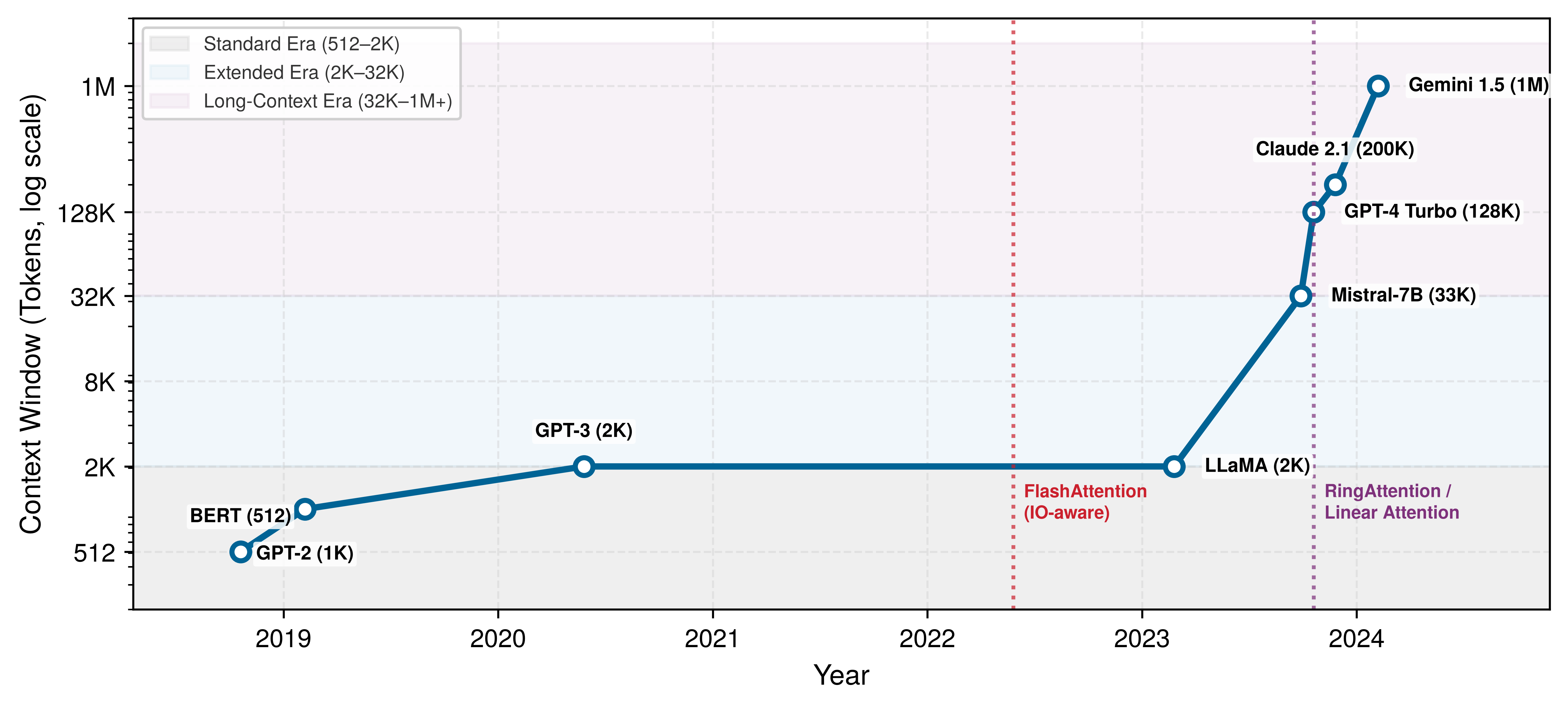
Figure 10: **Context Window Explosion**: Model context capacity (tokens, log scale) from early models (512 to 2K tokens) to modern long-context architectures (128K to 1M tokens). As context scales $1,000\times$, naive attention memory grows $1,000,000\times$ ($\mathcal{O}(S^2)$), driving the development of FlashAttention, sparse attention, and linear attention mechanisms.

Listing 8 presents a typical implementation, showing how self-attention derives queries, keys, and values from the same input sequence.

The preceding computational mapping shows how transformers process entire sequences in parallel. The picture changes at inference time, when the model generates tokens one at a time, a shift whose system consequences section 1.6.4 quantifies through the GPT-2 XL lighthouse.

System implications

The quadratic bottleneck analyzed in section 1.5.4 manifests differently across execution regimes. Full-sequence training and prefill compute all token positions together, whereas autoregressive decoding generates one token at a time. Their compute, memory, and data-movement bottlenecks depend on sequence length, batch size, model dimensions, implementation, and hardware.

Training: The quadratic compute wall

During training, all token positions can be processed in parallel, while dense attention’s score computation grows as $\mathcal{O}(S^2)$. For long sequences (for example, 32k tokens), materializing the $32k{\times}32k$ attention matrix requires gigabytes of memory per layer across multiple heads. This cost motivates optimizations like FlashAttention, which tiles computation to avoid materializing the full matrix in HBM. The hardware memory hierarchies (HBM, SRAM, register files) that make such tiling effective are detailed in Hardware Acceleration.

Small-batch autoregressive decoding: The memory bandwidth wall

Autoregressive decoding generates one token at a time and is often memory-bandwidth bound at batch one or small batch sizes. To generate a token, the system performs three broad operations:

Read model weights, with reuse determined by batching and the memory hierarchy (for example, a 70-billion-parameter model stores 140 GB of FP16 weights; GPT-2 XL makes the cost of that first step concrete).
Perform matrix-vector multiplications.
Read/write the KV Cache.

Listing 8: Self-Attention and Multi-Head Attention: Self-attention (top) derives $\mathbf{Q}$, $\mathbf{K}$, and $\mathbf{V}$ from the same input $\mathbf{X}$ through three projections, then computes attention as before. Multi-head attention (bottom) runs $N_{\text{heads}}$ parallel attention heads with dimension $d_k = d_{\text{model}}/N_{\text{heads}}$, then concatenates and projects. For GPT-2 (768-dim, 12 heads), each head operates on 64 dimensions, partitioning the projected feature dimension across heads while enabling diverse relationship patterns.

def self_attention_layer(X, W_Q, W_K, W_V, d_k):
    # X: input tensor (batch_size × seq_len × d_model)
    # W_Q, W_K, W_V: weight matrices (d_model × d_k)

    Q = matmul(X, W_Q)
    K = matmul(X, W_K)
    V = matmul(X, W_V)

    scores = matmul(Q, K.transpose(-2, -1)) / sqrt(d_k)
    attention_weights = softmax(scores, dim=-1)
    output = matmul(attention_weights, V)

    return output

def multi_head_attention(X, W_Q, W_K, W_V, W_O, num_heads, d_k):
    outputs = []
    for i in range(num_heads):
        head_output = self_attention_layer(
            X, W_Q[i], W_K[i], W_V[i], d_k
        )
        outputs.append(head_output)

    concat_output = torch.cat(outputs, dim=-1)
    final_output = matmul(concat_output, W_O)

    return final_output

The KV cache²¹ grows linearly with sequence length ($\mathcal{O}(N_L \times 2 \times N_{\text{heads}} \times S \times d_{\text{head}})$ per request, distinct from the $\mathcal{O}(S^2)$ attention score matrix during training), storing the key and value vectors for all previous tokens to avoid recomputing them (Pope et al. 2023; Kwon et al. 2023). For long contexts, this cache can become massive (for example, 100+ GB), and each decoding step reads prior keys and values. The resulting bandwidth pressure depends on context length, batching, attention architecture, cache layout, and hardware.

²¹ KV cache memory scaling: For a 7-billion-parameter transformer in FP16, model weights consume ~14 GB; a single request’s cache requires 32 layers $\times$ 2 (K,V) $\times$ 32 heads $\times$ 2,048 positions $\times$ 128 dimensions $\times$ 2 bytes, or about 1.07 GB. At 8 concurrent users, the cache is ~8.6 GB, a substantial addition to the weights, and grows linearly with context and concurrency, scaling throughput therefore forces choices such as grouped-query attention (Ainslie et al. 2023), shorter contexts, or KV paging and offloading (Kwon et al. 2023). Paging and offloading preserve model outputs, whereas grouped-query attention changes the architecture and shorter contexts change the information available to the model.

Ainslie, Joshua, James Lee-Thorp, Michiel de Jong, Yury Zemlyanskiy, Federico Lebron, and Sumit Sanghai. 2023. “GQA: Training Generalized Multi-Query Transformer Models from Multi-Head Checkpoints.” Proceedings of the 2023 Conference on Empirical Methods in Natural Language Processing, 4895–901. https://doi.org/10.18653/v1/2023.emnlp-main.298.

Kwon, Woosuk, Zhuohan Li, Siyuan Zhuang, Ying Sheng, Lianmin Zheng, Cody Hao Yu, Joseph Gonzalez, Hao Zhang, and Ion Stoica. 2023. “Efficient Memory Management for Large Language Model Serving with PagedAttention.” Proceedings of the 29th Symposium on Operating Systems Principles, 611–26. https://doi.org/10.1145/3600006.3613165.

This implementation reveals three key computational characteristics. Self-attention enables parallel processing across all positions in a full sequence. Dense score computation grows quadratically with sequence length, creating a long-sequence bottleneck. Autoregressive decoding adds a sequential dependency and can become bandwidth bound at small batch sizes.

This examination of MLPs, CNNs, RNNs, attention mechanisms, and transformers shows how each family addresses a different pattern through dense feature interactions, spatial locality, sequential dependencies, or input-dependent relationships. These families do not cover every production workload. Recommendation systems combine sparse embedding lookups, whose capacity and access distribution shape placement and caching, with dense layers that still require compute and bandwidth.

This hybrid matters at production scale: Meta reported that recommendation models accounted for most of its AI inference cycles (Gupta et al. 2020), even though such workloads receive less academic attention than language or vision models. Section 1.7 examines recommendation as the chapter’s final paradigm.

Gupta, Udit, Carole-Jean Wu, Xiaodong Wang, Maxim Naumov, Brandon Reagen, David Brooks, Bradford Cottel, et al. 2020. “The Architectural Implications of Facebook’s DNN-Based Personalized Recommendation.” 2020 IEEE International Symposium on High Performance Computer Architecture (HPCA), 488–501. https://doi.org/10.1109/HPCA47549.2020.00047.

Lighthouse 1.5: GPT-2 XL (bandwidth lighthouse)

Why it matters: GPT-2 XL exemplifies memory-bandwidth-bound batch-one decoding. In the weight-only model used here, each decoding step reads 6 GB of FP32 weights and performs matrix-vector operations. The resulting arithmetic intensity is about 0.5 FLOP/byte with FP32 weights or 1 FLOP/byte with FP16 weights. Batching can amortize this weight traffic, while KV-cache and activation traffic add to it. Table 6 summarizes the bandwidth lighthouse’s quantitative properties:

Table 6: GPT-2 XL Systems Profile: Weight-only estimates for batch-one autoregressive decoding. Under these assumptions, each step reads the model weights at roughly 0.5–1 FLOP/byte, so HBM bandwidth strongly constrains generation throughput.

Property	Value	System Implication
Parameters	1.5B	Weight loading dominates inference latency.
Model Size	6 GB (FP32)	Fits on one GPU but saturates HBM bandwidth.
Compute	3 GFLOP/token	Low per-token compute; bottleneck is data movement, not math.
Constraint	Memory Bandwidth	Weight-bound batch-one tokens/s depends strongly on HBM bandwidth.
Profile	Bandwidth-Bound (small-batch decoding)	Larger batches can amortize weight traffic and shift the bottleneck.

Self-Check: Question

Why do standard Transformer self-attention layers require explicit positional encodings (such as sinusoidal signals or learned positional embeddings) added to token embeddings?
1. Because matrix multiplication hardware cannot process tensors without fixed static padding across all dimensions.
2. Because layer normalization removes the mean and variance of token vectors, destroying word identity.
3. Because self-attention is mathematically permutation-invariant across sequence positions, meaning that without positional encodings, any permutation of the input tokens produces identical output representations.
4. Because positional encodings reduce the computational complexity of the attention matrix from $\mathcal{O}(S^2)$ to $\mathcal{O}(S)$.
Under a weight-only memory model in FP16 precision, an autoregressive language model generates 1 token per forward pass at batch size 1, performing approximately 2 FLOPs per parameter while streaming the entire weight matrix from High Bandwidth Memory (HBM). Calculate the theoretical arithmetic intensity of this decoding step and explain why it causes accelerator matrix units (Tensor Cores) to remain severely underutilized.
Order the sub-layer operations executed within a single standard Transformer encoder block during a forward pass:

Project input activations into Query, Key, and Value tensors via linear weight matrices
Compute multi-head scaled dot-product self-attention across all sequence positions
Apply residual skip connection addition and layer normalization to the attention output
Pass normalized representations through a position-wise two-layer feed-forward network (MLP)
Apply residual skip connection addition and layer normalization to the feed-forward output

A production serving system deploys a 32-layer transformer with 32 attention heads, head dimension $d_{\text{head}} = 128$, and context length $S = 2{,}048$ in FP16 precision (2 bytes per value). Calculate the memory footprint of the Key-Value (KV) cache for a single user request, and explain why KV-cache memory can surpass model weight memory under high concurrent batching.
During autoregressive language model inference, single-token generation at batch size 1 achieves near-peak GPU floating-point throughput (TFLOP/s) because the matrix-vector multiplication is highly optimized.
In a Multi-Head Attention layer with model dimension $d_{\text{model}} = 768$ and $N_{\text{heads}} = 12$ heads, what is the per-head dimension $d_k$, and how does multi-head projection affect total computational FLOP complexity compared to a single attention head operating on the full 768 dimensions?
1. The per-head dimension is $d_k = 768$, increasing total projection FLOPs by $12\times$ compared to a single head.
2. The per-head dimension is $d_k = 768 / 12 = 64$; running 12 heads of dimension 64 has the exact same total projection and score FLOP complexity as a single head of dimension 768, while enabling the model to jointly attend to information from 12 distinct representation subspaces.
3. The per-head dimension is $d_k = 12$, reducing total computational complexity by $64\times$.
4. Multi-head attention eliminates the output projection matrix $\mathbf{W}^O$, halving layer parameter count.

See Answers →

Sparse Architectures: RecSys

When a user opens a streaming service, the system must select a handful of recommendations from a catalog of millions—in under 50 milliseconds. The fundamental challenge is representing both users and items as dense vectors in a shared embedding space, then computing similarity at scale.

Unlike the architectures examined so far, which are typically compute bound or bandwidth bound, recommendation models are uniquely memory-capacity-bound due to their reliance on massive embedding tables. This distinction explains why the same GPU that processes transformers efficiently may struggle with recommendation workloads.

Pattern processing needs

The core challenge in RecSys is handling high-cardinality categorical features. A model might need to process User IDs (billions of unique users) and Item IDs (millions of videos or products). Raw IDs carry no geometry: user 1042 is not “near” user 1043 in any meaningful sense, and a neural network cannot infer similarity from the integer itself.

Embeddings solve the representation problem by mapping each ID to a dense vector called an embedding²² (Mikolov et al. 2013). The systems cost is that every lookup becomes a random read into a potentially enormous table. Recommendation workloads therefore inherit a capacity and bandwidth problem before the dense neural network layers begin.

²² Embedding: From the mathematical concept of embedding one space into another: neural embeddings map discrete tokens (user IDs, words) into continuous vector spaces where semantic similarity becomes geometric proximity. Word2vec popularized neural word embeddings in 2013. For systems, embedding tables create a distinctive memory access pattern: each lookup is a random read into a potentially terabyte-scale table, producing the sparse, bandwidth-bound workload that makes DLRM fundamentally different from compute-bound architectures like ResNet.

Mikolov, Tomas, Kai Chen, Greg Corrado, and Jeffrey Dean. 2013. “Efficient Estimation of Word Representations in Vector Space.” ICLR abs/1301.3781.

Algorithmic structure

The DLRM architecture (Naumov et al. 2019) standardizes this pattern as a four-stage pipeline split across dense and sparse regimes. Continuous features such as user age or time of day first flow through a bottom MLP, a compute-intensive but memory-light stage. The sparse stage then looks up categorical IDs in embedding tables, which is where the capacity wall appears:

Naumov, Maxim, Dheevatsa Mudigere, Hao-Jun Michael Shi, Jianyu Huang, Narayanan Sundaraman, Jongsoo Park, Xiaodong Wang, et al. 2019. “Deep Learning Recommendation Model for Personalization and Recommendation Systems.” arXiv Preprint arXiv:1906.00091.

Categorical features such as user ID or item ID are looked up in massive embedding tables. A table for one billion users with 128-dimensional vectors requires $10^9 \times 128 \times 4$ bytes $\approx$ 512 GB of memory, making this stage memory-intensive but compute-light because each lookup is essentially a memory copy. The interaction layer then combines dense vectors from the MLP with sparse embedding vectors, typically through dot products that capture user-item relationships. A top MLP finally processes the combined features to produce a probability such as click-through rate. This combination of dense and sparse computation makes DLRM the chapter’s recommendation lighthouse; section 1.7.3 quantifies the capacity-bound profile that results.

Computational mapping and system implications

DLRM’s computational mapping splits into two regimes that stress different hardware subsystems. The dense MLPs are standard GEMM operations, identical to the MLP computational mapping discussed in section 1.2.4 and handled efficiently by Tensor Cores. The sparse embedding lookups, however, are qualitatively different: they are index-based memory copies (gather operations) with no arithmetic, making them entirely memory-bandwidth bound at the operation level. This is distinct from the capacity constraint described earlier: the total size of the embedding tables is what makes the model memory-capacity-bound, whereas the speed of each individual gather is what makes the lookup operations memory-bandwidth bound. Because each training sample accesses a different set of embedding rows, the access pattern is effectively random, defeating caching and prefetching strategies that benefit CNNs and MLPs.

Lighthouse 1.6: DLRM (recommendation lighthouse)

Why it matters: DLRM exemplifies memory-capacity-bound workloads. Its massive embedding tables often exceed the memory of a single accelerator or server, so the system must decide where those tables live before it can optimize arithmetic throughput. The interaction layer then gathers selected embedding vectors and combines them with dense features, making capacity and irregular data movement the dominant constraints. This contrasts sharply with CNNs (compute bound) and transformers (memory-bandwidth bound), requiring different hardware and deployment choices. Table 7 summarizes the recommendation lighthouse’s quantitative properties:

Table 7: DLRM Systems Profile: Quantitative properties of the recommendation lighthouse and their system consequences. Billion-entry embedding tables push the model past single-device memory, creating a capacity-bound regime that the iron law does not directly address.

Property	Value	System Implication
Embedding Parameters	25B	Parameters $\times$ 4 bytes; dominates total model size.
Model Size	100 GB (FP32)	May exceed one device’s fast memory.
Constraint	Memory Capacity	Model size $> \text{Single GPU Memory}$.
Bottleneck	Irregular Data Movement	Gather operations dominate sparse feature processing.
Profile	Mixed (Sparse/Dense)	Combines memory-heavy lookups with compute-heavy MLPs.

Once embedding tables exceed one device, capacity—not arithmetic—becomes the first systems constraint. A ResNet-50 (102.4 MB) or even GPT-3 (350 GB) might fit on a single node, but industrial recommendation models can reach terabytes or petabytes because of their massive embedding tables. In iron law terms (Iron Law of ML Systems), neither $O$ nor $D_{\text{vol}}$ is the binding constraint—it is raw memory capacity that limits the system, a regime the iron law was not designed to capture.

DLRM embedding lookups can depend on vectors stored outside the local memory partition.

The architecture therefore breaks the single-device assumption that worked for the earlier families. A designer has three broad options, and each changes a different part of the system:

Shrink the tables: Compression, hashing, or pruning can reduce capacity pressure, but these techniques may lose information about rare users or items.
Move the tables: Embeddings can live in CPU memory, host memory, or a storage-backed feature system, but every lookup then pays a data-movement cost.
Partition the tables: Tables can be split across multiple memory resources so no one device stores the whole model, but each request may need vectors from several partitions.

Architecturally, DLRM turns recommendation into a capacity-management problem before it becomes a compute-optimization problem (for example, at 100 million IDs and 128 FP32 values per ID, one embedding table already consumes most of an 80 GB accelerator budget). The corresponding execution strategies include training-time partitioning in Model Training and hardware support for fast data movement in Hardware Acceleration.

One embedding table fits an 80 GB A100; a second breaches the capacity wall.

Napkin Math 1.2: The capacity wall

Problem: Consider a recommendation system for a store with 100M items using an embedding size of 128. How much memory does the item table alone require?

Math:

Table entries: 100M items.
Vector size: 128 elements.
Precision: FP32 (4 bytes per element).
Table size: 100M items $\times$ 128 $\times$ 4 bytes ≈ 51.2 GB.
Capacity share: 51.2 GB $\div$ 80 GB = 64 percent of device capacity.
Two-table check: Two tables at 64 percent each exceed 100 percent of device capacity.

Systems insight: A single embedding table for one feature (Items) already consumes 64 percent of an 80 GB A100 GPU. Adding a User table of the same size means the embedding tables no longer fit on a single 80 GB, motivating either smaller tables, off-device memory, or partitioning across memory resources. DLRM is capacity bound: our first question is not how many FLOPs the accelerator can deliver, but where the embedding state can physically reside.

Once the tables no longer fit on one device, sparse lookups cross memory and network boundaries. A request may need rows owned by several devices, so its dense MLP waits while the system gathers them. Within a node, this exchange stresses the accelerator interconnect; across nodes, it becomes many-to-many communication. The architectural consequence is that a DLRM’s memory layout determines the communication pattern that serving and training must pay, creating a fleet-scale coordination problem.

Checkpoint 1.4: DLRM and sparse scatter

Recommendation systems stress a different part of the machine than CNNs or transformers.

Capacity-bound: can you explain why embedding tables push DLRM into a memory capacity regime where “FLOPs” is not the binding constraint?
Sparse access: can you explain why embedding lookups behave like random memory gathers (low reuse) and therefore resist caching and prefetching?
Placement logic: if a single embedding table does not fit in fast device memory, can you describe which state must move, shrink, or be partitioned?
Data-movement bottleneck: can you explain why sparse embedding lookups can dominate even when the dense MLP has modest FLOP cost?

The five architecture families examined earlier (MLPs, CNNs, RNNs, transformers, and DLRM-style sparse models) appear to differ fundamentally, yet they share a striking convergence: many modern deep variants reuse a small set of primitives such as dense projections, normalization, skip connections, and gating. Every transformer block contains a feedforward MLP, and gating, invented for RNNs, reappears in mixture-of-experts routing. These building blocks are portable: they originated in one architecture family but migrated broadly because the problems they solve (gradient flow, activation stability, signal routing) recur across data types and inductive biases. For systems engineers, this portability is critical because it reveals which hardware optimizations transfer across workloads and which remain architecture-specific.

Self-Check: Question

In the Deep Learning Recommendation Model (DLRM) architecture, what is the primary computational role of the Interaction Layer?
1. It applies 2D convolutions over user and item IDs to extract hierarchical spatial features.
2. It normalizes categorical IDs across the batch using running mean and variance statistics.
3. It performs autoregressive token decoding to predict the next search query.
4. It computes pairwise dot products between the dense feature representations from the Bottom MLP and the sparse embedding vectors gathered from categorical tables to capture explicit feature interactions.
Explain why industrial recommendation models like DLRM are classified as memory-capacity-bound rather than compute-bound, and why the standard execution form of the Iron Law of ML Systems ($T_{\text{exec}} = D_{\text{vol}}/\text{BW} + O/(R_{\text{peak}} \cdot \eta_{\text{hw}}) + L_{\text{lat}}$) cannot directly determine whether a DLRM model can be deployed on a single accelerator.
Order the four primary computational stages executed during an end-to-end inference pass in a DLRM recommendation model:

Process continuous numerical features through the dense Bottom MLP to produce a dense representation
Look up sparse categorical IDs across embedding tables to gather discrete embedding vectors
Compute pairwise dot products (interactions) between the Bottom MLP output and all gathered embedding vectors
Concatenate interaction dot products with Bottom MLP features and pass through the Top MLP to predict click-through probability

An e-commerce recommendation system maintains an item embedding table with 100 million items ($10^8$) and a user embedding table with 1 billion users ($10^9$), each using 128-dimensional FP32 vectors (4 bytes per parameter). Calculate the memory footprint of each table, verify why they cannot fit on a single 80 GB A100 GPU, and describe two systems strategies to handle this capacity wall.
Why do sparse embedding table lookups in recommendation workloads resist standard hardware caching and memory prefetching mechanisms that accelerate CNNs and MLPs?
1. Because each incoming request queries arbitrary, non-contiguous row indices determined by sparse user and item IDs, producing irregular random gathers with minimal spatial locality across batches.
2. Because embedding tables are permanently encrypted in DRAM, preventing hardware prefetchers from reading address buses.
3. Because embedding lookups require performing high-order tensor contractions that stall CPU prefetch queues.
4. Because recommendation systems execute only on storage-class memory where hardware caching is disabled by operating system kernels.

See Answers →

Shared Building Blocks

A transformer block reuses several ideas born elsewhere: dense projections from MLPs, residual paths from deep CNNs, normalization for activation stability, and gating-like routing in later variants. The five architecture families differ in their data assumptions, but many of their engineering problems recur, so the practical question is which building blocks and optimizations transfer. Table 8 shows how these primitives accumulated as architectures grew more complex: each era inherited the tools of its predecessors while adding a mechanism for the next bottleneck.

Table 8: Cross-Architecture Building Blocks: Engineering primitives that originated in one architecture family and now recur across many modern designs. Each building block solves a recurring problem (gradient flow, activation stability, signal routing), though not every architecture uses every primitive.

Building Block	Born In	Problem Solved	Now Used In
GEMM	MLPs	Universal function approximation	All architectures (feedforward layers)
Parameter Sharing	CNNs	Spatial efficiency	Transformers (shared projections), RNNs (weight reuse across time)
Skip Connections	ResNets (CNNs)	Gradient flow at depth	Transformers, DenseNets, U-Nets, many modern deep networks
Normalization	CNNs (BatchNorm)	Activation stability	LayerNorm (Transformers), RMSNorm (root-mean-square normalization), GroupNorm (grouped channels)
Gating	LSTMs (RNNs)	Selective signal routing	Transformers (mixture-of-experts routing), GRUs, highway networks

Those portable building blocks were shaped by the hardware available at the time. LeNet-5 (LeCun et al. 1998) trained on CPUs with networks small enough to fit in megabytes of memory. AlexNet trained its 60-million-parameter network on two GTX 580 GPUs, mapping parallel convolutions to graphics hardware (Krizhevsky et al. 2012). ResNet-152 (He et al. 2016a) became trainable because residual connections and batch normalization improved optimization at depth, using available GPU training infrastructure rather than a specific memory-capacity threshold. Transformers (Vaswani et al. 2017) became practical on contemporary GPUs and later scaled dramatically as GPU/TPU memory bandwidth and distributed training infrastructure improved. This pattern continues: each building block exploits newly available computational resources while pushing against the limits of existing systems.

LeCun, Yann, Léon Bottou, Yoshua Bengio, and Patrick Haffner. 1998. “Gradient-Based Learning Applied to Document Recognition.” Proceedings of the IEEE 86 (11): 2278–324. https://doi.org/10.1109/5.726791.

Dense operations: The universal baseline

GEMM is the one primitive shared by every architecture in this chapter. While section 1.2 examined MLPs as dense pattern processors, the systems engineering legacy of GEMM extends far beyond MLPs. It is the feedforward layer inside every transformer block, the $1{\times}1$ pointwise convolution in MobileNets, the input and recurrent projections inside every RNN cell, and the bottom MLP in every DLRM.

MLPs introduced the GEMM-dominated computation profile that led GPU vendors to develop Tensor Cores. The backpropagation algorithm’s²³ memory access patterns, with its alternating forward and backward passes storing intermediate activations, influenced accelerator memory hierarchies. The batch processing paradigm pioneered for MLP training established the data-center-scale throughput optimization that defines modern ML infrastructure. These foundational patterns (dense matrix operations, gradient-based optimization, batch-oriented processing) appear in every architecture examined in this chapter, even when obscured by domain-specific terminology.

²³ Backpropagation: Rumelhart, Hinton, and Williams showed in 1986 how to efficiently apply the chain rule to train multi-layer networks; standard reverse-mode training retains the forward activations needed by the backward pass, so activation memory commonly grows with network depth. Checkpointing, recomputation, and offloading can reduce stored activations by trading additional computation or data movement. Activation storage, rather than weight storage, can therefore be the binding memory constraint that determines maximum feasible batch size on a given accelerator.

Dense connectivity also established the cost baseline that every subsequent architecture navigates. At $\mathcal{O}(n^2)$ parameters and operations for layers of width $n$, GEMM sets the reference point against which specialized architectures demonstrate efficiency gains. CNNs achieve spatial processing with $\mathcal{O}(k^2)$ parameters per location (where $k$ is kernel size), transformers trade parameter efficiency for dynamic computation with $\mathcal{O}(S^2)$ attention complexity, and sparse architectures like DLRM exploit embedding lookups to handle categorical dimensions that would explode dense layer sizes. Each innovation represents a different strategy for escaping the dense connectivity baseline, but none escapes GEMM itself—it reappears inside every architecture as the workhorse of feature transformation.

Skip connections: Solving the depth problem

Parameter sharing (born in CNNs) made deep networks efficient, but efficiency alone could not solve the challenges of training them. As practitioners attempted to build deeper CNNs for more complex tasks, they encountered a barrier that now confronts every deep architecture: the gradient flow problem. The mathematical foundation for skip connections starts with the failure modes of depth: vanishing gradients, exploding gradients, the limitations of ReLU, and the residual solution that enabled networks exceeding 100 layers.

The problem of depth

Backpropagation through $N_L$ layers applies the chain rule repeatedly; Gradient computation and backpropagation gives the formal derivation of backpropagation and the chain rule. For a deep network with layers $f_1, f_2, \ldots, f_{N_L}$, the gradient of the loss $\mathcal{L}$ with respect to the weights in layer 1 is: \[ \frac{\partial \mathcal{L}}{\partial W_1} = \frac{\partial \mathcal{L}}{\partial a_{N_L}} \cdot \frac{\partial a_{N_L}}{\partial z_{N_L}} \cdot \frac{\partial z_{N_L}}{\partial a_{N_L-1}} \cdot \ldots \cdot \frac{\partial z_2}{\partial a_1} \cdot \frac{\partial a_1}{\partial z_1} \cdot \frac{\partial z_1}{\partial W_1} \] where $z_\ell$ represents the preactivation and $a_\ell = \sigma(z_\ell)$ the postactivation output of layer $\ell$. The gradient becomes a product of $N_L$ terms, each depending on the activation function derivative $\sigma'(z_\ell)$.

Vanishing gradients create a silent training failure in deep architectures. For sigmoid activation functions, the derivative is $\sigma'(z) = \sigma(z)(1 - \sigma(z))$, with maximum value $\sigma'(0) = 0.25$. Through $N_L$ layers, the gradient magnitude is multiplied by approximately $(0.25)^{N_L}$. With such extreme attenuation, early layers receive infinitesimal gradient signals. Weight updates become negligible, effectively preventing these layers from training.

Exploding gradients are the catastrophic counterpart to vanishing gradients. Large singular values in layer Jacobians can amplify gradient directions repeatedly through depth. For example, if each Jacobian expands a shared direction by about 1.5, that component grows exponentially. Such growth can produce numerical overflow, not a number (NaN) values, extreme parameter updates, and training divergence. Unlike vanishing gradients, which silently prevent learning, exploding gradients can cause immediate training failure.

Quantitative analysis: Plain deep networks

Consider training a deep plain convolutional network on CIFAR-10 without architectural interventions. Even with ReLU activations, which have derivative one for positive inputs, optimization can degrade as depth increases. The original ResNet paper reported that a 56-layer plain network had substantially worse CIFAR-10 test error than a 20-layer plain network (about 13.6 percent vs. 8.8 percent), demonstrating that simply adding layers can make optimization worse despite greater representational capacity (He et al. 2016a).

This “degradation problem” is not overfitting. Deeper networks train worse than shallow ones, contradicting the intuition that more layers should provide more representational capacity.

Why ReLU helps but is not sufficient

ReLU activation ($\text{ReLU}(z) = \max(0, z)$) has derivative: \[ \text{ReLU}'(z) = \begin{cases} 1 & \text{if } z > 0 \\ 0 & \text{if } z \leq 0 \end{cases} \]

Through active paths $(z > 0)$, the derivative equals 1, avoiding gradient decay from the activation function. This represents significant improvement over sigmoid, enabling training of networks with 10–20 layers.

However, ReLU introduces a different problem: dead neurons. When $z \leq 0$, the gradient is exactly zero, blocking gradient flow through that activation. A poorly initialized neuron or large update can keep a ReLU unit negative across the training data, causing it to “die.” ReLU also does not solve gradient-flow issues arising from weight matrices themselves. Singular values far below or above one can still attenuate or amplify gradients through depth.

The residual solution

ResNet blocks introduce residual learning through skip connections that transform gradient flow. Equation 9 adds the identity path $\mathbf{x}$ to the residual mapping $\mathcal{F}(\mathbf{x})$. \[ \mathbf{y} = \mathcal{F}(\mathbf{x}) + \mathbf{x} \tag{9}\] where $\mathcal{F}(\mathbf{x})$ represents the residual function (typically two convolutional layers with batch normalization and ReLU) and $\mathbf{x}$ is the identity skip connection.

Theorem 1.2: Residual Jacobian conditioning

Analysis: Consider the network as a composition of functions $\mathbf{x}_{\ell+1} = f_\ell(\mathbf{x}_\ell)$. By the chain rule, the gradient at the input is the product of layer Jacobians $\mathbf{J}_\ell = \frac{\partial f_\ell}{\partial \mathbf{x}_\ell}$: \[ \frac{\partial \mathcal{L}}{\partial \mathbf{x}_0} = \frac{\partial \mathcal{L}}{\partial \mathbf{x}_{N_L}} \cdot \prod_{\ell=1}^{N_L} \mathbf{J}_\ell \]

For plain networks, $\mathbf{J}_\ell$ is arbitrary. The bound $\left\|\prod_\ell \mathbf{J}_\ell\right\|_2 \leq \prod_\ell \|\mathbf{J}_\ell\|_2$ means uniformly subunit norms force vanishing; conversely, $\sigma_{\min}(\prod_\ell \mathbf{J}_\ell) \geq \prod_\ell \sigma_{\min}(\mathbf{J}_\ell)$ means uniformly superunit minimum singular values force expansion. Mixed, non-normal Jacobians depend on singular vectors as well as eigenvalues, so spectral radius alone does not determine gradient behavior.

For ResNets, the layer function is $\mathbf{x}_{\ell+1} = \mathbf{x}_\ell + \mathcal{F}(\mathbf{x}_\ell)$, so the Jacobian is: \[ \mathbf{J}_\ell = \mathbf{I} + \frac{\partial \mathcal{F}}{\partial \mathbf{x}_\ell} \] where $\mathbf{I}$ is the identity matrix. If $\varepsilon_\ell=\|\mathcal{F}'_\ell\|_2<1$, then $1-\varepsilon_\ell \leq \sigma_{\min}(\mathbf{J}_\ell) \leq \sigma_{\max}(\mathbf{J}_\ell) \leq 1+\varepsilon_\ell$. Thus a block whose residual Jacobian is small is close to identity and locally well conditioned. Across many blocks these deviations may still compound, so the skip connection improves gradient flow without guaranteeing unit gain or preventing cancellation.

During backpropagation, the gradient flows through this addition: \[ \frac{\partial \mathcal{L}}{\partial \mathbf{x}} = \frac{\partial \mathcal{L}}{\partial \mathbf{y}} \cdot \frac{\partial \mathbf{y}}{\partial \mathbf{x}} = \frac{\partial \mathcal{L}}{\partial \mathbf{y}} \cdot \frac{\partial (\mathcal{F}(\mathbf{x}) + \mathbf{x})}{\partial \mathbf{x}} \]

Applying the chain rule: \[ \frac{\partial \mathcal{L}}{\partial \mathbf{x}} = \frac{\partial \mathcal{L}}{\partial \mathbf{y}} \cdot \left(\frac{\partial \mathcal{F}(\mathbf{x})}{\partial \mathbf{x}} + \mathbf{I}\right) = \frac{\partial \mathcal{L}}{\partial \mathbf{y}} \cdot \mathcal{F}'(\mathbf{x}) + \frac{\partial \mathcal{L}}{\partial \mathbf{y}} \]

This equation reveals the critical insight. The gradient divides into two contributions. The residual contribution, $\frac{\partial \mathcal{L}}{\partial \mathbf{y}}\mathcal{F}'(\mathbf{x})$, can be small, while the identity term contributes $\frac{\partial \mathcal{L}}{\partial \mathbf{y}}$ directly. The residual contribution can still partially cancel the identity term, but when $\mathcal{F}'(\mathbf{x})$ is small, the block Jacobian remains close to identity and improves conditioning. The additive path does not guarantee unattenuated gradients through arbitrary depth.

Gradient flow through multiple blocks

Through $N_L$ residual blocks, the gradient becomes: \[ \frac{\partial \mathcal{L}}{\partial \mathbf{x}_0} = \frac{\partial \mathcal{L}}{\partial \mathbf{x}_{N_L}} \cdot \prod_{\ell=1}^{N_L} \left(\mathcal{F}'_\ell(\mathbf{x}_\ell) + \mathbf{I}\right) \]

Each factor $(\mathcal{F}'_\ell + \mathbf{I})$ contains the identity term, keeping the factor near identity when the residual-branch Jacobian is small. Unlike plain networks, which multiply arbitrary layer Jacobians, ResNets multiply these near-identity factors. The deviations can still compound, but this structure improves conditioning and helps make networks with 100+ layers trainable.

Empirical validation at 56 layers

The ResNet CIFAR-10 experiments provide the empirical contrast: residual networks avoided the degradation seen in deeper plain networks and achieved lower training and test error as depth increased. In the same family of experiments, a 56-layer residual network reached about 7.0 percent test error, improving over the deeper plain network rather than degrading with depth (He et al. 2016a). The critical difference appears in gradient flow and optimization: identity shortcuts give later layers a direct path to refine earlier representations rather than forcing every layer to learn a complete transformation from scratch.

Skip connections improve gradient flow but can introduce system-level costs. The addition $\mathbf{y} = \mathcal{F}(\mathbf{x}) + \mathbf{x}$ requires the residual input to remain available until the paths merge. The incremental memory and runtime costs depend on tensor liveness, checkpointing, fusion, implementation, and architecture; the addition itself is usually small relative to the residual function $\mathcal{F}(\mathbf{x})$.

Residual networks avoided the degradation observed in comparable plain networks (He et al. 2016a). There is no fixed depth at which skip connections become necessary or insufficient: trainability also depends on initialization, normalization, optimization, layer type, and residual design (He et al. 2016b).

He, Kaiming, Xiangyu Zhang, Shaoqing Ren, and Jian Sun. 2016a. “Deep Residual Learning for Image Recognition.” 2016 IEEE Conference on Computer Vision and Pattern Recognition (CVPR), 770–78. https://doi.org/10.1109/cvpr.2016.90.

He, Kaiming, Xiangyu Zhang, Shaoqing Ren, and Jian Sun. 2016b. “Identity Mappings in Deep Residual Networks.” Computer Vision – ECCV 2016, 630–45. https://doi.org/10.1007/978-3-319-46493-0_38.

The gradient flow improvements from skip connections addressed one critical training challenge but left another: controlling activation distributions across layers. Even with skip connections improving gradient flow, poorly conditioned activations can destabilize training. Skip connections provide a direct gradient path; normalization can help control activation scale. This distinction explains why many deep architectures combine normalization with skip connections.

Normalization: Stabilizing activations at depth

Skip connections improve gradient flow to early layers; normalization helps control activation scale. Like skip connections, normalization is a portable building block: it was born as batch normalization in CNNs²⁴ (Ioffe and Szegedy 2015), evolved into layer normalization for transformers, and most recently simplified into RMSNorm²⁵ for efficient large language models. Many modern deep architectures use some variant. Understanding the mathematics of normalization reveals why these layers can materially improve deep-network training.

²⁴ Batch normalization (BatchNorm): The original normalization layer (Ioffe and Szegedy 2015), which re-scales activations using per-mini-batch statistics. In one ImageNet experiment, it reached the target accuracy with 14$\times$ fewer training steps. Its batch-size dependency and training-serving skew (switching from batch statistics to running averages at inference) are systems limitations that motivated alternatives: LayerNorm removed batch dependency for transformers, and RMSNorm removed mean centering.

Ioffe, Sergey, and Christian Szegedy. 2015. “Batch Normalization: Accelerating Deep Network Training by Reducing Internal Covariate Shift.” Proceedings of the 32nd International Conference on Machine Learning (ICML) 37: 448–56.

²⁵ RMSNorm (root mean square normalization): Introduced by Zhang and Sennrich (2019) at NeurIPS, RMSNorm simplifies LayerNorm by normalizing with the root mean square alone, dropping the mean-centering step. Across the paper’s tested models and implementations, RMSNorm reduced overall running time by 7–64 percent relative to LayerNorm. LLaMA-family and Mixtral-style transformer reports use RMSNorm (Touvron, Lavril, et al. 2023; Touvron, Martin, et al. 2023; Jiang et al. 2024), illustrating why one reduction pass can matter for transformer inference latency.

Zhang, Biao, and Rico Sennrich. 2019. “Root Mean Square Layer Normalization.” Advances in Neural Information Processing Systems (NeurIPS).

Touvron, Hugo, Thibaut Lavril, Gautier Izacard, Xavier Martinet, Marie-Anne Lachaux, Timothée Lacroix, Baptiste Rozière, et al. 2023. “LLaMA: Open and Efficient Foundation Language Models.” arXiv Preprint arXiv:2302.13971.

Touvron, Hugo, Louis Martin, Kevin Stone, Peter Albert, Amjad Almahairi, Yasmine Babaei, Nikolay Bashlykov, et al. 2023. “Llama 2: Open Foundation and Fine-Tuned Chat Models.” arXiv Preprint arXiv:2307.09288.

Jiang, A. Q., A. Sablayrolles, A. Roux, A. Mensch, B. Savary, C. Bamford, D. S. Chaplot, et al. 2024. “Mixtral of Experts.” arXiv Preprint arXiv:2401.04088.

Batch normalization: Definition and formulation

Batch normalization normalizes activations using statistics computed over the mini-batch for each feature or channel during training. For fully connected activations, the averaging axis is the batch. For convolutional activations, implementations typically compute per-channel statistics over both the batch and spatial positions. For a mini-batch $\mathcal{B} = \{x_1, \ldots, x_B\}$ of activations at a particular layer, the transformation proceeds in two stages.

First, compute the batch statistics: \[ \mu_{\mathcal{B}} = \frac{1}{B}\sum_{i=1}^{B} x_i \qquad \sigma_{\mathcal{B}}^2 = \frac{1}{B}\sum_{i=1}^{B} (x_i - \mu_{\mathcal{B}})^2 \]

Then, over the batch, normalize and apply learnable scale and shift. The normalization step in equation 10 centers and scales activations, while equation 11 applies learnable parameters that allow the network to recover the identity transformation if optimal: \[ \hat{x}_i = \frac{x_i - \mu_{\mathcal{B}}}{\sqrt{\sigma_{\mathcal{B}}^2 + \epsilon}} \tag{10}\] \[ y_i = \gamma \hat{x}_i + \beta \tag{11}\]

The parameters $\gamma$ (scale) and $\beta$ (shift) are learned during training, while $\epsilon$ (typically $10^{-5}$) prevents division by zero. The affine transform restores learned scale and shift flexibility, but fixed $\gamma$ and $\beta$ cannot exactly invert varying statistics for every batch. Normalization often permits larger learning rates in some architectures and training regimes, which can accelerate convergence relative to an otherwise comparable unnormalized network.

Theorem 1.3: Normalization Jacobian conditioning

Analysis: The mathematical insight into why normalization aids training lies in how it conditions the Jacobian matrix of the layer. For the current batch, consider the gradient of the normalized output with respect to the input: \[ \frac{\partial \hat{x}_i}{\partial x_j} = \frac{1}{\sqrt{\sigma_{\mathcal{B}}^2 + \epsilon}} \left( \delta_{ij} - \frac{1}{B} - \frac{(x_i - \mu_{\mathcal{B}})(x_j - \mu_{\mathcal{B}})}{B(\sigma_{\mathcal{B}}^2 + \epsilon)} \right) \] where $\delta_{ij}$ is the Kronecker delta. This Jacobian couples examples within the batch, with scale set by $1/\sqrt{\sigma_{\mathcal{B}}^2+\epsilon}$; the subsequent affine scale $\gamma$ multiplies it. It has zero directions associated with batchwise shift invariance, so there is no universal positive eigenvalue bound such as $[0.5,2.0]$.

Batch normalization can improve optimization empirically by standardizing intermediate scales, but it does not by itself prevent vanishing or exploding gradients through an entire network. Its quantitative effect depends on architecture, batch statistics, optimization, and parameterization rather than a universal two-to-fourfold gradient range.

Layer normalization: Architecture independence

While batch normalization enabled training of much deeper CNNs, it introduced a problematic dependency on batch statistics. This creates issues for small batch sizes (noisy statistics), varying sequence lengths (incompatible batch dimensions), and inference (requires running mean/variance estimation). Layer normalization addresses these limitations by normalizing across features rather than across the batch (Ba et al. 2016).

For an input vector $\mathbf{x} \in \mathbb{R}^{d_{\text{model}}}$ with $d_{\text{model}}$ features: \[ \mu_{\text{LN}} = \frac{1}{d_{\text{model}}}\sum_{i=1}^{d_{\text{model}}} x_i \qquad \sigma_{\text{LN}}^2 = \frac{1}{d_{\text{model}}}\sum_{i=1}^{d_{\text{model}}} (x_i - \mu_{\text{LN}})^2 \]

Equation 12 defines the complete layer normalization operation, where $\odot$ denotes element-wise multiplication: \[ \text{LayerNorm}(\mathbf{x}) = \frac{\mathbf{x} - \mu_{\text{LN}}}{\sqrt{\sigma_{\text{LN}}^2 + \epsilon}} \odot \boldsymbol{\gamma} + \boldsymbol{\beta} \tag{12}\]

Layer normalization normalizes each sample independently, making the operation invariant to batch size and suitable for autoregressive models where per-sample independence is required (batch statistics would leak information across samples). This architectural difference explains why transformers universally adopt layer normalization: the self-attention mechanism processes sequences of varying length, and autoregressive generation requires each position to be normalized independently of batch composition.

Comparative analysis: When to use each variant

The choice between normalization variants depends on computational context. Table 9 summarizes the key trade-offs. BatchNorm typically stores learned scale/shift parameters plus nonlearned running mean/variance buffers; LayerNorm computes per-sample statistics at runtime and typically stores learned scale/shift parameters but no running-statistic buffers.

Batch size constraints emerge because batch normalization estimates statistics from the values available for each channel. Small effective sample counts can make those statistics noisy, but the threshold depends on architecture, spatial dimensions, task, and implementation. This constraint impacts memory-limited scenarios such as high-resolution images or large models.

The computational cost of computing mean and variance adds $\mathcal{O}(B \times d_{\text{model}})$ operations per batch normalization layer for batch size $B$ and feature dimension $d_{\text{model}}$. For layer normalization, the cost is $\mathcal{O}(d_{\text{model}})$ per sample. RMSNorm reduces this further by eliminating the mean computation.

Table 9: Normalization Variant Comparison: Different normalization techniques trade off between computational efficiency, batch size sensitivity, and architectural compatibility. RMSNorm (Zhang and Sennrich 2019), used in LLaMA-family and other efficient transformer architectures (Touvron, Lavril, et al. 2023; Touvron, Martin, et al. 2023), omits mean centering: $\text{RMSNorm}(\mathbf{x}) = \mathbf{x} / \sqrt{\frac{1}{d_{\text{model}}}\sum_i x_i^2 + \epsilon} \cdot \boldsymbol{\gamma}$.

Characteristic	BatchNorm	LayerNorm	RMSNorm
Normalization Axis	Batch and, for CNNs, spatial positions	Feature dimension	Feature dimension
Batch Size Dependency	High (noisy for small batches)	None	None
Typical Use Case	CNNs, vision models	Transformers, RNNs	LLaMA, efficient transformers
Computation Cost	Higher (mean + variance)	Higher (mean + variance)	Lower (RMS only)
Training/Inference	Different (running stats)	Identical	Identical

Operational differences between training vs. inference require explicit mode switching for batch normalization, which exhibits different behavior between training (batch statistics) and inference (running statistics). Incorrect mode handling is a common source of training-serving skew. Layer normalization behaves identically in both modes, simplifying deployment.

Skip connections and normalization solve depth-related problems—gradient flow and activation stability, respectively. The third portable building block, gating, solves a different problem entirely: selectively routing information through the network.

Gating: Controlling information flow

Gating mechanisms were born in RNNs, where early sequence models hit a “temporal barrier”: gradients vanished or exploded through long sequences, revealing that simple recurrence was insufficient for long-term dependencies. LSTMs²⁶ (Hochreiter and Schmidhuber 1997) and GRUs²⁷ (Cho et al. 2014) addressed this by introducing gates: small MLPs that learn to control the flow of information through the network, acting as differentiable valves that selectively protect, forget, or route signals.

²⁶ LSTM (long short-term memory): Invented by Hochreiter and Schmidhuber in 1997, LSTMs introduced a “Constant Error Carousel,” a gated cell state that protects error signals from exponential decay during backpropagation through time. The systems cost of this solution: a standard LSTM computes input, forget, and output gates plus a candidate cell update, giving roughly four affine transformations per time step vs. one in a vanilla RNN. This compute overhead explains why transformers, which solve long-range dependencies through parallelizable attention, replaced LSTMs in many large-scale language workloads.

Hochreiter, Sepp, and Jürgen Schmidhuber. 1997. “Long Short-Term Memory.” Neural Computation 9 (8): 1735–80. https://doi.org/10.1162/neco.1997.9.8.1735.

²⁷ GRU (gated recurrent unit): Cho et al. (2014) describes a gated hidden unit for encoder-decoder translation that uses reset and update gates to control how the hidden state is updated. Relative to an LSTM’s input, forget, and output gates plus candidate cell update, this gives a simpler gated recurrence. The broader systems lesson: architectural simplification can reduce state and matrix operations when it preserves task performance, a principle that recurs in efficiency-oriented designs from MobileNet to distilled transformers.

Cho, Kyunghyun, Bart van Merrienboer, Dzmitry Bahdanau, and Yoshua Bengio. 2014. “On the Properties of Neural Machine Translation: Encoder-Decoder Approaches.” Proceedings of SSST-8, Eighth Workshop on Syntax, Semantics and Structure in Statistical Translation, 103–11. https://doi.org/10.3115/v1/w14-4012.

Bahdanau, Dzmitry, Kyunghyun Cho, and Yoshua Bengio. 2015. “Neural Machine Translation by Jointly Learning to Align and Translate.” International Conference on Learning Representations (ICLR).

The key insight is that gating is not an RNN-specific technique. It is a general principle of using one learned signal to modulate another learned signal. Highway Networks applied the idea to feedforward layers, letting the network decide whether to transform an input or pass it through, which made them an important precursor to skip connections. Attention uses the same principle at the sequence level: encoder-decoder attention (Bahdanau et al. 2015), originally introduced for machine translation, learns which source positions should influence each output position. In transformers, the softmax attention weights become the routing signal that controls how much each position contributes to the output, while later large-scale variants extend the same idea to explicit expert routing. The portability of gating reinforces the central theme: the building blocks that matter most are not tied to any single architecture but solve universal problems—in this case, the problem of selectively routing information through deep, complex networks.

Synthesis: How transformers recombine everything

The transformer recombines several building blocks discussed earlier. A full transformer block combines the residual-path idea illustrated in figure 11 with dense projections, normalization, and attention gating. Dense GEMM operations in MLP-style feedforward networks process features between attention layers. Residual paths wrap every sub-layer, enabling gradient flow through deep stacks. LayerNorm, evolved from the same stabilization problem that BatchNorm addressed in CNNs, stabilizes activations at each sub-layer (Ba et al. 2016). Softmax attention weights then gate how much each position contributes, while mixture-of-experts variants extend the same routing idea to explicit expert selection.

Ba, Jimmy Lei, Jamie Ryan Kiros, and Geoffrey E. Hinton. 2016. “Layer Normalization.” arXiv Preprint arXiv:1607.06450.

\begin{tikzpicture}[line join=round,font=\small\sffamily]
\tikzset{%
  Line/.style={line width=1.0pt,black!50,text=black},
  Box/.style={align=center,
    inner xsep=2pt,
    node distance=2,
    draw=BlueLine,
    line width=0.75pt,
    fill=BlueL,
    text width=24mm,
    minimum width=24mm, minimum height=10mm
  },
  op/.style={circle, draw=GreenLine, minimum size=9mm,fill=GreenL,line width=0.75pt},
  >={Latex[length=2mm]},line/.style={-latex, thick},
do path picture/.style={%
    path picture={%
      \pgfpointdiff{\pgfpointanchor{path picture bounding box}{south west}}%
        {\pgfpointanchor{path picture bounding box}{north east}}%
      \pgfgetlastxy\x\y%
      \tikzset{x=\x/2,y=\y/2}%
      #1
    }
  },
plus/.style={do path picture={
    \draw [black,line cap=round, line width=1pt] (-3/5,0) -- (3/5,0) (0,-3/5) -- (0,3/5);
  }}
}
%
\node[Box] (in) {Weight Layer};
\node[Box, right=5 of in] (hidden) {Weight Layer};
\node[op] (relu1) at ($(in)!0.5!(hidden)$) {ReLU};
\node[circle,draw,minimum size=7mm,node distance=1.65,right=of hidden,plus,
draw=BrownLine,fill=BrownL,line width=0.75pt] (add) {};
\node[op, below=0.7 of add] (relu2) {ReLU};
%
\draw[Line,-latex] (in) -- (relu1);
\draw[Line,-latex] (relu1) -- (hidden);
\draw[Line,-latex] (hidden) -- (add);
\draw[Line,-latex] (add) -- (relu2);
\draw[Line,-latex] (relu2) -- ++(1.7,0);
%  Feedback (identity)
\draw[Line,latex-] (in.west) --coordinate(SR) ++(-1.5,0) node[left] {$\mathbf{x}$};
\draw[Line,-latex] (SR) --++(0,0.9)  -| node[pos=0.25,above]{$\mathbf{x}$ identity}(add);
%
\node[below=2pt of relu2] {$\mathcal{F}(\mathbf{x}) + \mathbf{x}$};
\node[below=2pt of relu1] {$\mathcal{F}(\mathbf{x})$};
\end{tikzpicture}

Figure 11: Residual Connection Block: The skip connection implements $\mathbf{y} = \text{ReLU}(\mathcal{F}(\mathbf{x}) + \mathbf{x})$, creating an identity shortcut that bypasses the weight layers before the final nonlinearity. During backpropagation, gradients flow through both the residual path (via $\mathcal{F}'(\mathbf{x})$) and the identity path (via $\mathbf{I}$ before the final nonlinearity), helping gradients reach early layers even in 100+ layer networks. This architectural pattern enabled very deep residual CNNs and became central in transformer blocks and many other modern architectures.

This recombination is not accidental. The transition from RNNs to transformers represents a decisive engineering shift from sequential to parallel state management. Replacing time-step dependencies with global, data-dependent routing (attention) moves sequence models from $\mathcal{O}(S)$ sequential complexity to $\mathcal{O}(1)$ sequential steps for information flow between any two positions, enabling full use of accelerator parallelism. The other building blocks, however, carried over unchanged: GEMM, skip connections, and normalization remain essential across all families.

This portability recurs in later architectures. Vision Transformers²⁸ adapt the transformer to images while maintaining all four building blocks (Dosovitskiy et al. 2021). GPT-3, for example, scales up these transformer patterns and uses alternating dense and locally banded sparse attention while still relying on the same core primitives (Brown et al. 2020). Practical implementation challenges and optimizations are explored in Model Compression.

²⁸ Vision transformers (ViTs): Google’s 2020 ViT paper split $224{\times}224$ images into $16{\times}16$ patches (196 “tokens”) and applied standard transformer attention. ViTs replace CNN’s local convolutions with $\mathcal{O}(S^2)$ global attention over patch tokens. In the original study, large-scale pretraining improved ViT’s competitiveness, illustrating how data and compute can compensate for weaker spatial inductive bias (Dosovitskiy et al. 2021).

Dosovitskiy, Alexey, Lucas Beyer, Alexander Kolesnikov, Dirk Weissenborn, Xiaohua Zhai, Thomas Unterthiner, Mostafa Dehghani, et al. 2021. “An Image Is Worth 16x16 Words: Transformers for Image Recognition at Scale.” International Conference on Learning Representations (ICLR).

Brown, Tom B., Benjamin Mann, Nick Ryder, Melanie Subbiah, Jared Kaplan, Prafulla Dhariwal, Arvind Neelakantan, et al. 2020. “Language Models Are Few-Shot Learners.” Advances in Neural Information Processing Systems 33: 1877–901. https://doi.org/10.48550/arxiv.2005.14165.

Table 10 makes this synthesis concrete. Transformers retain the core GEMM operations common to all architectures but introduce content-dependent all-to-all reductions through attention, blending the broadcast operations of MLPs with the gather and reduce operations of more dynamic architectures.

Table 10: Primitive Utilization Across Architectures: Every architecture uses GEMM, but they differ in memory access patterns, data movement (broadcast to gather+reduce), and parallelism. Transformers combine dense tiled QKV access with attention-specific reductions, which is why they stress both the GEMM units and the reduction path at once.

Primitive Type	MLP	CNN	RNN	Transformer
Computation	Dense GEMM	Convolution	Sequential GEMM	GEMM + Attention
Memory Access	Sequential	Strided	Sequential + State	Tiled QKV streams
Data Movement	Broadcast	Sliding window	Temporal broadcast	Gather + Reduce
Parallelism	High	High	Low (time deps)	High (positions)

For systems engineers, this building-block perspective separates portable optimizations from architecture-specific ones. GEMM tiling and mixed-precision compute benefit every architecture. Skip connection memory management applies to any residual network. Normalization kernel fusion helps CNNs and transformers alike. Attention-specific optimizations remain tied to attention’s memory pattern, but even those build on the same underlying GEMM and memory-access primitives. To understand why these optimizations transfer, section 1.9 lowers the shared layers to the primitives the machine executes.

Self-Check: Question

In a residual block implementing $\mathbf{y} = \mathcal{F}(\mathbf{x}) + \mathbf{x}$, how does the additive identity shortcut mathematically condition the layer Jacobian $\mathbf{J} = \frac{\partial \mathbf{y}}{\partial \mathbf{x}}$ during backpropagation to prevent vanishing gradients in 100+ layer networks?
1. The shortcut forces the residual function $\mathcal{F}(\mathbf{x})$ to have zero weights, turning the network into an immutable linear identity operator.
2. The Jacobian takes the form $\mathbf{J} = \mathbf{I} + \frac{\partial \mathcal{F}}{\partial \mathbf{x}}$, ensuring that even when residual path derivatives $\frac{\partial \mathcal{F}}{\partial \mathbf{x}}$ are small, the block Jacobian remains near the identity matrix $\mathbf{I}$, providing an unattenuated gradient pathway across layers.
3. The shortcut doubles the singular values of the weight matrix at every layer, ensuring gradients explode exponentially rather than vanish.
4. The shortcut eliminates the backpropagation chain rule by replacing gradient updates with forward-only finite differences.
Compare Batch Normalization (BatchNorm) and Layer Normalization (LayerNorm) along two critical systems dimensions: (a) sensitivity to mini-batch size during training, and (b) operational differences between training and inference (including training-serving skew).
Order the historical emergence and cross-architecture migration of deep learning building blocks from earliest innovation to modern synthesis:

Dense linear operations (GEMM) established as the universal baseline in Multilayer Perceptrons
Local parameter sharing and spatial weight reuse introduced in Convolutional Neural Networks
Gating mechanisms (input/forget/output gates) introduced in LSTMs to control signal propagation
Additive identity skip connections and Batch Normalization introduced in ResNets to enable 100+ layer depth
Transformers synthesize GEMM projections, skip connections, layer normalization, and attention gating into a unified parallel architecture

Modern efficient large language models (such as the LLaMA family) frequently replace standard LayerNorm with ____, which omits the mean-centering step and scales activations using only the root mean square of feature values, reducing memory reduction passes and improving inference latency.
Why did the Transformer architecture adopt Layer Normalization rather than Batch Normalization as its standard normalization building block?
1. Because Batch Normalization requires $10\times$ more learnable parameters than Layer Normalization.
2. Because Layer Normalization can only run on CPU hardware, matching early NLP training cluster setups.
3. Because Transformers process variable-length sequences where batch padding distorts mini-batch statistics, and autoregressive generation requires each sequence position to be normalized independently of batch composition.
4. Because the Universal Approximation Theorem forbids using Batch Normalization with multi-head attention mechanisms.

See Answers →

Computational Primitives

Portable building blocks still lower to a smaller set of operations; those primitives determine what hardware must execute. A ResNet-50 forward pass executes billions of multiply-accumulate operations; a transformer attention layer moves gigabytes through memory hierarchies; a DLRM lookup scatters random reads across terabyte-scale tables. Despite their architectural differences, all three reduce to a small set of computational primitives that hardware and software must actually execute. Synthesizing the per-architecture system implications from earlier sections into a unified view reveals common optimization opportunities.

Each primitive represents an operation that cannot be decomposed further while maintaining its essential characteristics. Understanding these operations reveals where performance bottlenecks arise on specific hardware and guides the optimization strategies detailed in Hardware Acceleration.

Core computational primitives

The core primitive question is which execution pattern an architecture forces the system to optimize: dense tensor math, repeated local reuse, or input-dependent routing. Matrix multiplication, sliding window operations, and dynamic computation recur across the families because each preserves a distinct performance profile when lowered to hardware. They are primitive in the engineering sense: decomposing them further would erase the performance characteristics a system must optimize.

Matrix multiplication is the dense tensor-math path. Multiplying a matrix of inputs by a matrix of weights computes weighted combinations, the core operation of neural networks (recall the reference MLP layer from section 1.2.3). This path appears everywhere: MLPs use it directly for layer computations, CNNs can lower convolutions into matrix multiplications, and transformers use it extensively in their attention mechanisms. Figure 12 shows one row-major arrangement: each sliding-window position unfolds into a row of the transformed matrix.

\begin{tikzpicture}[line join=round,font=\sffamily\small]
\tikzset{
Line/.style={line width=1.0pt,VioletLine,text=black},
  mymatrix/.style={
    matrix of nodes,
    nodes={
      draw,
      fill=orange!40,
      minimum size=8mm,
      text centered,
      execute at begin node=\strut, % za vertikalno poravnanje
      text depth=0.25ex,
      text height=1.25ex,
    },
    column sep=-\pgflinewidth,
    row sep=-\pgflinewidth,
    nodes in empty cells
  }
}
%MA1
\begin{scope}[local bounding box=MA1,shift={(0,0)}]
    \matrix[mymatrix,
  column 1/.style={nodes={fill=cyan!30}},
  column 2/.style={nodes={fill=cyan!30}},
  column 3/.style={nodes={fill=cyan!30}},
  column 4/.style={nodes={fill=cyan!30}},](M1){%
1&  2 &4&5&10&11&13&14 \\
2& 3  &5&6&11&12&14&15 \\
4& 5  &7&8&13&14&16&17 \\
5& 6  &8&9&14&15&17&18 \\
      };
\node[draw=red,inner sep=-2pt,rounded corners=8pt,
yshift=0mm,fill=none,fit=(M1-1-1)(M1-1-4),line width=1.5pt](F1){};
\node[draw=red,inner sep=-2pt,rounded corners=8pt,
yshift=0mm,fill=none,fit=(M1-2-5)(M1-2-8),line width=1.5pt](F3){};
\node[above=3pt of M1]{Transformed GEMM};
\end{scope}
%MA2
\begin{scope}[local bounding box=MA2,shift={($(MA1.north west)+(-3,-1)$)}]
    \matrix[mymatrix,
 nodes={fill=green!40}](M2){%
1& 2 \\
3& 4 \\
      };
\node[draw=red,inner sep=-2pt,rounded corners=8pt,
yshift=0mm,fill=none,fit=(M2-1-1)(M2-2-2),line width=1.5pt](F5){};
\end{scope}
%MA3
\begin{scope}[local bounding box=MA3,shift={($(MA1.south west)+(-3,0.5)$)}]
    \matrix[mymatrix,
 nodes={
      fill=yellow!30}](M3){%
5& 6 \\
7& 8 \\
      };
\node[below=3pt of M3]{Filter Kernels};
\end{scope}
%MA4
\begin{scope}[local bounding box=MA4,shift={($(M2-2-1.north west)+(-2.75,0.5)$)}]
    \matrix[mymatrix,
 nodes={
      fill=cyan!30}](M4){%
1& 2&3 \\
4& 5&6 \\
7& 8&9 \\
      };
\node[draw=red,inner sep=-2pt,rounded corners=8pt,
yshift=0mm,fill=none,fit=(M4-1-1)(M4-2-2),line width=1.5pt](F2){};
\node[below=3pt of M4]{Input feature maps};
\end{scope}
%MA5
\begin{scope}[local bounding box=MA4,shift={($(M3-2-1.north west)+(-2.75,-0.5)$)}]
    \matrix[mymatrix,
 nodes={ fill=orange!40}](M5){%
10& 11&12 \\
13& 14&15 \\
16& 17&18 \\
      };
\node[draw=red,inner sep=-2pt,rounded corners=8pt,
yshift=0mm,fill=none,fit=(M5-1-2)(M5-2-3),line width=1.5pt](F4){};
\end{scope}
%MA6
\begin{scope}[local bounding box=MA6,shift={($(MA1.east)+(1.98,0)$)}]
    \matrix[mymatrix,
 nodes={fill=green!40},
row 5/.style={nodes={fill=yellow!30}},
row 6/.style={nodes={fill=yellow!30}},
row 7/.style={nodes={fill=yellow!30}},
row 8/.style={nodes={fill=yellow!30}}](M6){%
1\\ 2 \\ 3\\ 4 \\ 5\\ 6\\7\\8\\
      };
\node[draw=red,inner sep=-2pt,rounded corners=8pt,
yshift=0mm,fill=none,fit=(M6-1-1)(M6-4-1),line width=1.5pt](F6){};
\end{scope}
%%
\draw[Line,-latex](F5)--++(0,2.5)-|(F6);
\draw[Line,-latex](F2)--++(0,1.2)-|(F1);
\draw[Line,-latex](F4)--++(0,-2.0)-|(F3);
\node[font=\huge] at($(M1.east)!0.5!(M6.west)$){$\times$};
\coordinate(SR)at($(M2-2-2.south east)!0.65!(M3-1-2.north east)$);
\node[single arrow, draw=black,thick, fill=VioletL,
      minimum width = 20pt, single arrow head extend=3pt,
      minimum height=11mm]at($(SR)!0.5!(M1.west)$) {};
\end{tikzpicture}

Figure 12: im2col Transformation: Converts convolution to GEMM by unfolding image patches into a dense matrix. The two $3{\times}3$ input feature maps produce four sliding-window positions, represented here as rows of a $4{\times}8$ matrix; the two $2{\times}2$ filter kernels stack into an $8{\times}1$ column. Their product yields the four output positions. Lowering can exploit optimized matrix kernels but expands memory by an amount that depends on kernel size, stride, padding, and implementation, so its performance benefit is workload dependent.

The im2col²⁹ (image to column) technique is the bridge that turns sliding-window locality into the matrix-multiply path. It unfolds overlapping image patches into a dense matrix. In the row-major arrangement in figure 12, each sliding-window position becomes a row and the stacked filter values form a column; transposed conventions are also common. This allows the convolution operation to be expressed as a standard GEMM operation.

²⁹ im2col (image to column): Rather than being a new learning algorithm, im2col-style lowering is an implementation technique used by CNN frameworks and libraries such as Caffe and cuDNN (Jia et al. 2014; Chetlur et al. 2014): it converts convolutions into standard GEMM calls by unfolding overlapping patches into matrix columns. The trade-off is memory: in a simple fully materialized stride-1 $K{\times}K$ transform, interior input elements can appear in up to $K^2$ columns (9 times for $3{\times}3$ filters), though borders, stride, padding, tiling, and direct-convolution algorithms reduce the realized expansion. This memory-for-simplicity exchange explains why mobile frameworks (TFLite, NNAPI) prefer direct convolution, while data center GPUs with abundant HBM may use GEMM-oriented lowering when it improves throughput.

Jia, Yangqing, Evan Shelhamer, Jeff Donahue, Sergey Karayev, Jonathan Long, Ross Girshick, Sergio Guadarrama, and Trevor Darrell. 2014. “Caffe: Convolutional Architecture for Fast Feature Embedding.” Proceedings of the 22nd ACM International Conference on Multimedia, 675–78. https://doi.org/10.1145/2647868.2654889.

Chetlur, Sharan, Cliff Woolley, Philippe Vandermersch, Jonathan Cohen, John Tran, Bryan Catanzaro, and Evan Shelhamer. 2014. “cuDNN: Efficient Primitives for Deep Learning.” arXiv Preprint arXiv:1410.0759.

The optimization trade-off is pragmatic: im2col spends memory to use mature GEMM implementations such as cuBLAS, MKL, and OpenBLAS. The transformation duplicates data where windows overlap, and whether lowering outperforms a direct convolution depends on the workload, implementation, and target hardware.

Structured and unstructured sparsity are treated in Pruning; hardware-aware sparse execution and algorithm-hardware co-design are treated in Hardware Acceleration.

Sliding window operations are the local-reuse path. They compute local relationships by applying the same operation to chunks of data. A $3{\times}3$ convolution filter slides across the input, generating one output per window position (for example, $26{\times}26$ windows for a $28{\times}28$ input with stride 1). Modern hardware accelerators implement this through specialized memory access patterns and data buffering schemes that optimize data reuse. For example, TPUs use systolic arrays³⁰ where data flows systematically through processing elements, allowing each input value to be reused across multiple computations without repeatedly accessing off-chip memory.

³⁰ Systolic array: Named for the heart’s rhythmic contraction, the array’s lockstep “pulse” of data through a grid of processors directly implements the efficient data reuse required by sliding window operations. By passing input values between neighboring processors, an expensive round-trip to off-chip DRAM is avoided for every single multiplication in the convolution. This is critical for efficiency, as a single off-chip memory access can cost over 100$\times$ more energy than a floating-point multiply-accumulate, and still more relative to low-precision arithmetic.

Content-dependent weighting is an adaptive-routing path. In dense transformer attention, each query’s weights depend on the input, but the tensor shapes and dense computation graph remain regular and are commonly implemented with GEMMs and tiled reductions. Sparse attention and mixture-of-experts routing can additionally make the executed operations data dependent.

Real architectures combine these paths, which is why primitive-level reasoning is a design tool rather than a taxonomy. A transformer layer uses matrix multiplications of shape $[S,d_{\text{model}}] \times [d_{\text{model}},d_{\text{proj}}]$ for feature projections and computes an $S{\times}S$ score pattern for dense attention. Some variants use sliding windows or data-dependent sparse routing. The interaction between primitives creates specific demands on system design, from memory hierarchy organization to computation scheduling.

The core computational primitives above explain why certain hardware features exist (Tensor Cores for matrix multiplication) and why software frameworks organize computations in particular ways (batching similar operations together). Computational primitives, however, tell only part of the story: the way operations access memory often determines real-world performance more than the operations themselves.

Memory access primitives

The next optimization decision is whether the primitive can feed the compute units predictably. Memory access often constitutes the primary bottleneck in ML systems: even a matrix multiplication unit capable of thousands of operations per cycle will remain idle if data is not available in time. Accessing data from DRAM typically requires hundreds of cycles, while on-chip computation requires only a few, making data movement a first-order energy constraint.

The relevant access patterns are sequential access, strided access, and random access because they determine how much of the memory stream the system can predict and reuse. Each pattern creates different demands on the memory system and offers different opportunities for optimization. Critically, each incurs vastly different energy costs based on the preceding principle.

Systems Perspective 1.2: The energy cost of data movement

A core systems principle: moving data costs more than computing on it. A floating-point multiply-accumulate operation consumes approximately 1–5 pJ depending on process node (for example, ~4.6 pJ at 45 nm (Horowitz 2014)), while fetching a 32-bit operand from off-chip DRAM costs hundreds of pJ in the same reference model. Even conservative estimates put off-chip DRAM access tens to hundreds of times above arithmetic, explaining why memory access patterns, not just FLOP counts, determine real-world efficiency.

Revisit the preceding architectures through this energy lens: MLPs have low data reuse (each weight loaded once per sample) and are therefore energy-dominated by DRAM traffic. CNNs reuse filter weights across spatial positions, amortizing load cost over $H \times W$ applications; the very locality that makes them compute-bound also makes them energy-efficient. RNNs reuse weights across time steps (high temporal reuse) but pay repeated hidden-state read/write costs at each step. Transformers combine pairwise score computation with key-value movement, making dense full-sequence attention compute-quadratic; implementation and tiling determine auxiliary memory traffic and energy. These energy profiles directly track the bottleneck column in table 3.

This principle underlies later optimization strategies: Quantization and Precision shows how quantization reduces bits moved per value, pruning eliminates unnecessary data movement, and tiling keeps working sets in faster, lower-energy caches.

Sequential access is the simplest, most efficient pattern, and the most energy-favorable. Consider an MLP performing matrix multiplication: it accesses weight matrices and input vectors in contiguous order. This pattern maps well to modern memory systems; DRAM can operate in burst mode for sequential reads (reaching on the order of hundreds of GB/s in modern GPUs), and hardware prefetchers can effectively predict and fetch upcoming data. Software frameworks optimize for this by ensuring data is laid out contiguously in memory and aligning data to cache line boundaries.

Strided access appears prominently in CNNs, where each output position needs to access a window of input values at regular intervals. Each output position requires accessing nine input values (for a $3{\times}3$ filter) with a stride matching the input width. While less efficient than sequential access, hardware supports this through pattern-aware caching strategies and specialized memory controllers. Software frameworks often transform these strided patterns into sequential access through data layout reorganization, where the im2col transformation in deep learning frameworks converts convolution’s strided access into efficient matrix multiplications.

Random access poses the greatest challenge for system efficiency. Sparse embedding lookups in recommendation models illustrate this challenge. Each request may touch a different set of table rows, defeating predictable streaming and causing cache misses or irregular memory latency. Dense transformer attention is different. Its weights are content-dependent, but Q, K, and V are stored in contiguous tensors and optimized kernels tile those tensors through SRAM/registers while reducing over the sequence. The systems challenge for dense attention is therefore quadratic score computation and reduction structure, not arbitrary address-random fetches.

Table 11 quantifies how these different memory access patterns contribute to the overall memory requirements of each architecture, comparing MLPs, CNNs, RNNs, and transformers across parameter storage, activation storage, and scaling behavior.

Table 11: Memory Access Complexity: Different neural network architectures exhibit varying memory access patterns and storage requirements, impacting system performance and scalability. Parameter storage depends on model dimensions, while activation storage represents a significant runtime cost. The transformer’s $\mathcal{O}(B S^2)$ term describes materialized attention scores in a naïve implementation; tiled exact-attention kernels can avoid retaining that full matrix.

Architecture	Input Dependency	Parameter Storage	Activation Storage	Scaling Behavior
MLP	Linear	$\mathcal{O}(N_{\text{in}} \times d_{\text{width}})$	$\mathcal{O}(B \times d_{\text{width}})$	Predictable
CNN	Constant w.r.t. resolution	$\mathcal{O}(K^2 C_{\text{in}} C_{\text{out}})$	$\mathcal{O}(B \times H_{\text{img}} \times W_{\text{img}} \times C)$	Efficient
RNN	Linear	$\mathcal{O}(d_{\text{hidden}}^2)$	$\mathcal{O}(B \times S \times d_{\text{hidden}})$	Challenging
Transformer	Quadratic attention	$\mathcal{O}(d_{\text{model}}^2 + d_{\text{model}} d_{\text{ff}})$ per block	$\mathcal{O}(B \times S^2)$ attention, plus $\mathcal{O}(B S d_{\text{model}})$ activations	Problematic

Where:

$N_{\text{in}}$: Input size
$d_{\text{width}}$: Layer width
$B$: Batch size
$K$: Kernel size
$C$: Number of channels
$C_{\text{in}}, C_{\text{out}}$: Input and output channels
$H_{\text{img}}$: Height of input feature map (CNN)
$W_{\text{img}}$: Width of input feature map (CNN)
$d_{\text{hidden}}$: RNN hidden-state dimension
$S$: Sequence length
$d_{\text{model}}$: Transformer model dimensionality

Table 11 captures where data lives and how access patterns scale. The complementary table 12 that follows captures how much computation each architecture demands, including forward-pass FLOPs, parallelization potential, and the resulting bottleneck. Together, the two tables answer the systems questions “how much work?” and “how does the memory system handle it?”, providing a resource profile that informs design decisions such as choosing memory hierarchy configurations and developing memory optimization strategies.

The impact of these patterns becomes clear when we consider data reuse opportunities. In CNNs, each input pixel participates in multiple convolution windows (typically nine times for a $3{\times}3$ filter), making effective data reuse necessary for performance. Modern GPUs provide multi-level cache hierarchies (L1, L2, shared memory) to capture this reuse, while software techniques like loop tiling ensure data remains in cache once loaded.

Working set size, the amount of data needed simultaneously for computation, varies dramatically across architectures. An MLP layer might need only a few hundred KB (weights plus activations), while a transformer processing long sequences can require several MB just for storing attention patterns. These differences directly influence hardware design choices, like the balance between compute units and on-chip memory, and software optimizations like activation checkpointing, which saves memory by recomputing selected activations during backpropagation instead of storing all of them, or attention approximation techniques.

Table 12: Computational Complexity Comparison: Scaling behaviors and resource requirements for major neural network architectures. Variables: $d_{\text{in}}$ = input dimension, $d_{\text{out}}$ = output dimension, $d_{\text{model}}$ = transformer model dimension, $d_{\text{hidden}}$ = RNN hidden-state dimension, $k$ = kernel size, $c$ = channels, $H_{\text{img}}, W_{\text{img}}$ = spatial dimensions, $S$ = sequence length (time steps), $B$ = batch size. The bottleneck column identifies the primary performance-limiting factor in typical deployments. For transformers, the $\mathcal{O}(S^2)$ memory term assumes materialized attention scores; tiled exact-attention kernels can avoid retaining that full matrix.

Architecture	Parameters	Forward Pass	Memory	Parallelization	Bottleneck
MLPs	$\mathcal{O}(d_{\text{in}} \times d_{\text{out}})$ per layer	$\mathcal{O}(d_{\text{in}} \times d_{\text{out}})$ per layer	$\mathcal{O}(d_{\text{in}}d_{\text{out}})$ weights $\mathcal{O}(B d_{\text{out}})$ activations	Excellent Matrix ops parallel	Memory bandwidth
CNNs	$\mathcal{O}(k^2 \times c_{\text{in}} \times c_{\text{out}})$ per layer	$\mathcal{O}(H_{\text{img}} \times W_{\text{img}} \times k^2 \times c_{\text{in}} \times c_{\text{out}})$	$\mathcal{O}(H_{\text{img}} \times W_{\text{img}} \times c)$ features $\mathcal{O}(k^2 \times c^2)$ weights	Good Spatial independence	Often compute throughput; bandwidth for depthwise or small-batch cases
RNNs	$\mathcal{O}(d_{\text{hidden}}^2+d_{\text{hidden}} \times d_{\text{in}})$ total	$\mathcal{O}(S \times d_{\text{hidden}}^2)$ for $S$ time steps	$\mathcal{O}(d_{\text{hidden}})$ recurrent state (inference); $\mathcal{O}(S d_{\text{hidden}})$ activations (training)	Poor Sequential deps	Sequential deps
Transformers	$\mathcal{O}(d_{\text{model}}^2)$ QKV/O projections plus $\mathcal{O}(d_{\text{model}}d_{\text{ff}})$ feed-forward layers	$\mathcal{O}(S^2 \times d_{\text{model}} + S \times d_{\text{model}}^2)$ per layer	$\mathcal{O}(S^2)$ attention $\mathcal{O}(S \times d_{\text{model}})$ sequences	Excellent (positions) Limited by memory	Memory $(S^2)$

Understanding these memory access patterns is essential as architectures evolve. The shift from CNNs to transformers, for instance, has driven the development of hardware with larger on-chip memories and more advanced caching strategies to handle increased working sets and more dynamic access patterns. Future architectures will likely continue to be shaped by their memory access characteristics as much as their computational requirements.

Data movement primitives

Memory access patterns describe where data resides, but a complementary dimension determines system performance: the flow of information between components. Data movement primitives characterize these flows. As established in section 1.9.2, data movement often dominates both time and energy budgets, making these flow patterns critical optimization targets.

The data-movement decision is fan-out and fan-in: whether one value must reach many consumers, many values must converge, or different values must be routed to different destinations. Figure 13 separates the four recurring patterns: broadcast, scatter, gather, and reduction. Broadcast operations send the same data to multiple destinations simultaneously. In matrix multiplication with batch size 32, each weight must be broadcast to process different inputs in parallel. Modern hardware supports this through specialized interconnects and hardware multicast capabilities, with bandwidth on the order of hundreds of GB/s in high-end accelerator interconnects, while some accelerators also use dedicated on-chip broadcast fabrics. Software frameworks optimize broadcasts by restructuring computations (like matrix tiling) to maximize data reuse.

\begin{tikzpicture}[line join=round,font=\sffamily,scale=0.8, every node/.append style={transform shape}]
\definecolor{Ballcol}{RGB}{172,245,164}
\colorlet{Ballcol}{gray!20}%brown!60!black!20}%magenta!20!magenta!20}%orange!30}%blue!30!cyan!80}
\tikzset{%
LineA/.style={line width=0.75pt,black,-latex},
ALine/.style={line width=0.75pt,black,latex-}
}

\tikzset{
  box/.pic={
    \pgfkeys{/box/.cd, #1}
\foreach \x in {1,...,\columns}{
    \foreach \y in {1,...,\rows}{
        %
        \node[draw=none, fill=\ffill, minimum width=\cellsize, inner sep=0pt,
                    minimum height=\cellheight, line width=\llinewidth] (cell-\x-\y\br) at (\x*\cellsize,-\y*\cellheight) {};
      }
     }
   }
 }

\pgfkeys{
  /box/.cd,
  cellsize/.store in=\cellsize,
  llinewidth/.store in=\llinewidth,
  cellheight/.store in=\cellheight,
  columns/.store in=\columns,
  br/.store in=\br,
  ffill/.store in=\ffill,
  rows/.store in=\rows,
  columns=1,
  rows=3,
  br=A,
  ffill=red,
  cellsize=2mm,
  cellheight=5mm,
  llinewidth=0pt
}
\def\radius{6mm}

\begin{scope}[scale=1, every node/.append style={transform shape},
local bounding box=B1,shift={($(0,0)+(0,0)$)}]
\foreach \x in {1,2,3,4}{
\pgfmathsetmacro{\xcord}{1.6*\x}
\coordinate (1B-\x) at (\xcord,0);
\filldraw[fill=Ballcol] (\xcord,0) circle (\radius);
\pic[shift={(-0.20,0.5)}] at (1B-\x) {box={columns=1,rows=1,br=A,ffill=red}};
}
\pgfmathsetmacro{\xcenter}{(1.6*1 + 1.6*4)/2} %
\coordinate (1CB) at (\xcenter,-2.5);
\filldraw[fill=Ballcol]  (1CB) circle (\radius);
\pic[shift={({-0.20,0.5})}] at (1CB) {box={columns=1,rows=1,br=A,ffill=red}};

\foreach \x in {1}{
  \foreach \y in {1,2,3,4}{
    \edef\from{\x CB}
    \edef\to{1B-\y}
\path let
    \p1 = (\from),
    \p2 = (\to),
    \n1 = {atan2(\y2-\y1,\x2-\x1)}
  in
    coordinate (from) at ($ (\from) + (\n1:\radius) $)
    coordinate (to) at ($ (\to) + (\n1+180:\radius) $);
  \draw[LineA] (from) -- node[inner sep=0pt](L\x){}(to);
  }
}
\node[below=7mm of 1CB]{Broadcast};
\end{scope}

\begin{scope}[scale=1, every node/.append style={transform shape},
local bounding box=B2,shift={($(0,0)+(11,0)$)}]

\foreach \x/\col in {1/red,2/yellow,3/green,4/myblue}{
\pgfmathsetmacro{\xcord}{1.6*\x}
\coordinate (2B-\x) at (\xcord,0);
\filldraw[fill=Ballcol]  (\xcord,0) circle (\radius);
\pic[shift={(-0.20,0.5)}] at (2B-\x) {box={columns=1,rows=1,br=A,ffill=\col}};
}
\pgfmathsetmacro{\xcenter}{(1.6*1 + 1.6*4)/2} % Sredina između prve i četvrte lopte
\coordinate (2CB) at (\xcenter,-2.5);
\filldraw[fill=Ballcol]  (2CB) circle (\radius);

\foreach \x/\col in {1/red,2/yellow,3/green,4/myblue}{
\pgfmathsetmacro{\xcord}{0.2*\x}
\pic[shift={({-0.70,0.5})}] at ($(2CB)+(\xcord,0)$) {box={columns=1,rows=1,br=A,ffill=\col}};
}

\foreach \x in {2}{
  \foreach \y in {1,2,3,4}{
    \edef\from{\x CB}
    \edef\to{2B-\y}
\path let
    \p1 = (\from),
    \p2 = (\to),
    \n1 = {atan2(\y2-\y1,\x2-\x1)}
  in
    coordinate (from) at ($ (\from) + (\n1:\radius) $)
    coordinate (to) at ($ (\to) + (\n1+180:\radius) $);
  \draw[LineA] (from) -- node[inner sep=0pt](L\x){}(to);
  }
}
\node[below=7mm of 2CB]{Scatter};
\end{scope}
%%%%%
\begin{scope}[scale=1, every node/.append style={transform shape},
local bounding box=B3,shift={($(0,0)+(0,-4.75)$)}]

\foreach \x/\col in {1/red,2/yellow,3/green,4/myblue}{
\pgfmathsetmacro{\xcord}{1.6*\x}
\coordinate (3B-\x) at (\xcord,0);
\filldraw[fill=Ballcol]  (\xcord,0) circle (\radius);
\pic[shift={(-0.20,0.5)}] at (3B-\x) {box={columns=1,rows=1,br=A,ffill=\col}};
}
\pgfmathsetmacro{\xcenter}{(1.6*1 + 1.6*4)/2} % Sredina između prve i četvrte lopte
\coordinate (3CB) at (\xcenter,-2.5);
\filldraw[fill=Ballcol]  (3CB) circle (\radius);

\foreach \x/\col in {1/myred,2/yellow,3/green,4/myblue}{
\pgfmathsetmacro{\xcord}{0.2*\x}
\pic[shift={({-0.70,0.5})}] at ($(3CB)+(\xcord,0)$) {box={columns=1,rows=1,br=A,ffill=\col}};
}

\foreach \x in {3}{
  \foreach \y in {1,2,3,4}{
    \edef\from{\x CB}
    \edef\to{3B-\y}
\path let
    \p1 = (\from),
    \p2 = (\to),
    \n1 = {atan2(\y2-\y1,\x2-\x1)}
  in
    coordinate (from) at ($ (\from) + (\n1:\radius) $)
    coordinate (to) at ($ (\to) + (\n1+180:\radius) $);
  \draw[ALine] (from) -- node[inner sep=0pt](L\x){}(to);
  }
}
\node[below=7mm of 3CB]{Gather};
\end{scope}
%%%%%%%
\begin{scope}[scale=1, every node/.append style={transform shape},
local bounding box=B4,shift={($(0,0)+(11,-4.75)$)}]

\foreach \x/\col in {1/1,2/3,3/5,4/7}{
\pgfmathsetmacro{\xcord}{1.6*\x}
\coordinate (4B-\x) at (\xcord,0);
\filldraw[fill=Ballcol]  (\xcord,0) circle (\radius);
%\pic[shift={(-0.20,0.5)}] at (4B-\x) {box={columns=1,rows=1,br=A,ffill=\col}};
\node[]at(4B-\x){\large\col};
}
\pgfmathsetmacro{\xcenter}{(1.6*1 + 1.6*4)/2}
\coordinate (4CB) at (\xcenter,-2.5);
\filldraw[fill=Ballcol]  (4CB) circle (\radius);
\node[]at(4CB){\large 16};

\foreach \x in {4}{
  \foreach \y in {1,2,3,4}{
    \edef\from{\x CB}
    \edef\to{4B-\y}
\path let
    \p1 = (\from),
    \p2 = (\to),
    \n1 = {atan2(\y2-\y1,\x2-\x1)}
  in
    coordinate (from) at ($ (\from) + (\n1:\radius) $)
    coordinate (to) at ($ (\to) + (\n1+180:\radius) $);
  \draw[ALine] (from) -- node[inner sep=0pt](L\x){}(to);
  }
}
\node[below=7mm of 4CB]{Reduction};
\end{scope}
\end{tikzpicture}

Figure 13: Data Movement Primitives: Four fundamental patterns govern information flow in neural network computation. Broadcast (top-left) replicates a single value to all destinations, used when sharing weights across batch elements. Scatter (top-right) distributes distinct elements to different destinations, enabling work partitioning. Gather (bottom-left) collects distributed values to a single location, as in attention pooling. Reduction (bottom-right) combines multiple values through aggregation (sum, max), appearing in gradient synchronization and attention scoring. The energy cost of data movement (see section 1.9.2) makes these patterns critical optimization targets.

Scatter operations distribute different elements to different destinations. When parallelizing a $512{\times}512$ matrix multiplication across accelerator cores, each core receives a subset of the computation. This parallelization is important for performance but challenging, as memory conflicts and load imbalance can reduce efficiency substantially. Hardware provides flexible high-bandwidth interconnects (often in the hundreds of GB/s class within a node), while software frameworks employ specialized work distribution algorithms to maintain high utilization. In large language models, mixture-of-experts architectures expose a far more demanding scatter pattern: a learned gating network routes each token to a small subset of expert sub-networks distributed across accelerators, requiring all-to-all communication that scales with the number of devices. Unlike the predictable tile-to-core scatter in matrix tiling, expert routing is data-dependent, so load imbalance across experts is common and can leave most accelerator capacity idle while a handful of hot experts become bottlenecks. This communication cost is a primary constraint on scaling such models to hundreds of experts.

Gather operations collect data from multiple sources. Dense transformer attention combines information from every key-value position, but implementations operate on regular dense tensors and commonly tile these reductions for locality. Irregular random gathers instead arise in workloads such as sparse embeddings, graph neighborhoods, and data-dependent routing.

Reduction operations combine multiple values into a single result through operations like summation. When computing attention scores in transformers or layer outputs in MLPs, efficient reduction is essential. Hardware implements tree-structured reduction networks (reducing latency from $\mathcal{O}(n)$ to $\mathcal{O}(\log n)$), while software frameworks use optimized parallel reduction algorithms that can achieve near-theoretical peak performance.

In practice, these patterns combine in layered ways. For each sequence and attention head in a transformer attention operation with sequence length 512 and batch size 32, the computation involves broadcasting query vectors ($512{\times}64$ elements), gathering relevant keys and values ($512{\times}512{\times}64$ elements), and reducing attention scores ($512{\times}512$ elements). The batch dimension multiplies each of these counts by 32.

The evolution from CNNs to transformers has increased reliance on gather and reduction operations, driving hardware innovations like more flexible interconnects and larger on-chip memories. As models grow (some now exceeding 100 billion parameters), efficient data movement becomes an architecture constraint rather than an implementation afterthought, leading to innovations like near-memory processing and targeted data flow optimizations.

System design impact

The computational, memory access, and data movement primitives explored earlier become system design constraints when they force resources to be allocated in silicon and software. Matrix-heavy workloads justify tensor units; random and gather-heavy workloads justify memory hierarchy and interconnect investment. The way these primitives influence hardware design, create common bottlenecks, and drive trade-offs turns architecture selection into infrastructure planning.

The most visible result is specialized hardware. The prevalence of matrix multiplications and convolutions in deep learning has led to the development of TPUs³¹ and Tensor Cores in GPUs, which are specifically designed to perform these operations efficiently. Hardware Acceleration examines how these specialized units map architectural primitives to silicon, from systolic arrays for GEMM to dataflow engines for convolution.

³¹ TPU (tensor processing unit): Google’s first TPU maps matrix multiplication onto a large systolic array, trading general-purpose features such as caches and complex control flow for domain-specific inference efficiency (Jouppi et al. 2017). The architectural lesson needed here is qualitative: when one primitive dominates a workload, dedicated data paths and local reuse can outperform general-purpose flexibility. Hardware Acceleration develops the precision choices, hardware specifications, and performance trade-offs.

Jouppi, Norman P., Cliff Young, Nishant Patil, David Patterson, Gaurav Agrawal, Raminder Bajwa, Sarah Bates, et al. 2017. “In-Datacenter Performance Analysis of a Tensor Processing Unit.” Proceedings of the 44th Annual International Symposium on Computer Architecture, ISCA ’17, 1–12. https://doi.org/10.1145/3079856.3080246.

Memory systems have also evolved in response to deep learning primitives. The need to support both sequential and random access patterns efficiently has driven the development of multi-level memory hierarchies. HBM–3D-stacked DRAM delivering 2–3 TB/s of bandwidth, over 20$\times$ standard server RAM–has become common in AI accelerators to support high data-movement requirements, especially for operations such as transformer attention. On-chip memory hierarchies have grown in complexity, with multiple levels of caching and scratchpad memories–programmer-controlled SRAM that trades cache convenience for explicit data movement and predictable locality–to support the diverse working set sizes of different neural network layers.

The data movement primitives have particularly influenced the design of interconnects and on-chip networks. The need to support efficient broadcasts, gathers, and reductions has led to the development of more flexible and higher-bandwidth interconnects. Some AI chips now feature specialized networks-on-chip designed to accelerate common data movement patterns in neural networks.

The system implications of these primitives span hardware, software, and performance considerations. Table 13 turns the primitive-to-system mapping into a design checklist: each row links an architectural primitive to the hardware support, software optimization, and bottleneck it tends to create. Despite the specialized hardware that these primitives have motivated, several bottlenecks persist. Memory bandwidth often remains a key limitation, particularly for models with large working sets or those that require frequent random access. The energy cost of data movement, especially between off-chip memory and processing units, continues to be a significant concern. For large-scale models, the communication overhead in distributed training can become a bottleneck, limiting scaling efficiency.

Table 13: Primitive-Hardware Co-Design: Efficient machine learning systems require tight integration between algorithmic primitives and underlying hardware. Common primitives map to specific hardware accelerations and software optimizations, each presenting distinct implementation challenges. Specialized hardware such as Tensor Cores addresses computational demands of matrix multiplication and sliding windows, while software techniques like batching and dynamic graph execution further enhance performance.

Primitive	Hardware Impact	Software Optimization	Key Challenges
Matrix Multiplication	Tensor Cores	Batching, GEMM libraries	Parallelization, precision
Sliding Window	Specialized datapaths	Data layout optimization	Stride handling
Dynamic computation	Flexible routing	Dynamic graph execution	Load balancing
Sequential Access	Burst mode DRAM	Contiguous allocation	Access latency
Random Access	Large caches	Memory-aware scheduling	Cache misses
Broadcast	Specialized interconnects	Operation fusion	Bandwidth
Gather/Scatter	High-bandwidth memory	Work distribution	Load balancing

The same primitive mapping also determines energy budgets. Each architectural pattern exhibits distinct energy characteristics that inform deployment decisions and optimization strategies for data center and edge systems.

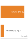
Moving a 32-bit value from DRAM costs far more energy than one FP32 multiply.

Large batched GEMMs in MLPs can achieve excellent arithmetic intensity, but small-batch MLP inference often has low reuse and can spend much of its energy on data movement. The reference FP32 multiply costs approximately 3.7 pJ/FLOP, while one 32-bit DRAM access costs 640 pJ (Horowitz 2014), about 173× as much per event. This ratio alone does not prove total dominance because workload energy also depends on operation counts, transfer counts, and reuse. Data movement can nevertheless dominate low-reuse inference, making bandwidth and locality important energy targets. This energy gap has driven accelerator designers to maximize on-chip SRAM capacity, keeping frequently reused weights and activations closer to compute and avoiding the DRAM penalty. Architectures that keep their working sets or active tiles on-chip, whether through tiled SRAM banks or wafer-scale integration, reduce inference energy by avoiding repeated off-chip transfers.

Convolutional operations reduce energy consumption through data reuse but exhibit variable efficiency depending on implementation. Im2col-based convolution implementations trade memory for simplicity; a fully materialized lowering can multiply temporary storage and memory traffic, up to $K^2$ for stride-1 $K{\times}K$ filters away from the borders. Direct convolution implementations can achieve substantially better energy efficiency by eliminating redundant data movement, particularly for larger kernel sizes where im2col duplication is most severe.

Sequential processing in RNNs creates energy efficiency opportunities through temporal data reuse. The constant memory footprint of RNN hidden states allows aggressive caching strategies that can dramatically reduce DRAM access energy for long sequences by keeping the recurrent state in on-chip SRAM. The sequential dependencies limit parallelization opportunities, often resulting in suboptimal hardware utilization and higher energy per operation.

Attention mechanisms in transformers can exhibit high energy consumption per operation due to data movement and, in naive implementations, stored attention matrices (the quadratic bottleneck from section 1.5.4). Attention’s data movement can raise energy per useful FLOP compared with standard matrix multiplication, making long-sequence processing expensive without implementations such as FlashAttention.

These energy profiles make primitive support a deployment trade-off. Optimizing for the dense matrix operations common in MLPs and CNNs might come at the cost of flexibility needed for the more dynamic computations in attention mechanisms. Supporting large working sets for transformers might require sacrificing energy efficiency.

The right balance depends on the target workloads and deployment scenarios. Understanding the nature of each primitive guides the development of both hardware and software optimizations in ML systems, allowing designers to make informed decisions about system architecture and resource allocation.

The analysis of architectural patterns, computational primitives, and system implications provides the conceptual foundation for understanding how architectures work and what they cost. The practical selection problem is to choose an architecture for a specific problem under specific deployment constraints. This selection process must consider not only algorithmic performance but also the deployment constraints covered in ML Systems and the lifecycle requirements introduced in ML Workflow.

Self-Check: Question

Based on Horowitz’s reference energy models for CMOS hardware, roughly how does the energy required to read a single 32-bit word from off-chip DRAM compare to executing a single 32-bit floating-point multiply-accumulate (MAC) arithmetic operation?
1. Off-chip DRAM access requires exactly the same energy as a 32-bit floating-point multiply-accumulate operation (~4.6 pJ each).
2. A 32-bit floating-point multiply-accumulate operation requires over $100\times$ more energy (~640 pJ) than reading from DRAM (~4.6 pJ).
3. Off-chip DRAM access requires roughly $2\times$ less energy than arithmetic because DRAM capacitors store passive electrostatic charge.
4. Off-chip DRAM access requires over $100\times$ more energy (~640 pJ) than executing an FP32 arithmetic operation (~4.6 pJ), making data movement rather than arithmetic the dominant energy cost in memory-heavy workloads.
Define the four fundamental collective data movement primitives (Broadcast, Scatter, Gather, Reduction) and identify one concrete neural network operation that exemplifies each primitive.
The im2col transformation converts a 2D convolution into a standard matrix multiplication (GEMM) without requiring any additional memory or duplicated data buffers in RAM.
Google’s Tensor Processing Unit (TPU) accelerates matrix multiplication and 2D convolution by organizing processing elements into a 2D ____ array, where activations and weights flow rhythmically across adjacent hardware registers to maximize data reuse without repeatedly accessing external DRAM.
Explain the architectural difference between hardware-managed caches (such as L1/L2 caches in general-purpose CPUs/GPUs) and programmer-controlled scratchpad SRAM in specialized AI accelerators, and explain why scratchpads provide superior energy efficiency and predictable latency for regular neural network tensor workloads.
Which memory access pattern is the most energy-efficient and hardware-friendly for memory controllers due to DRAM burst-mode capability and hardware prefetching?
1. Contiguous sequential memory access, because it maximizes DRAM burst transfer efficiency, cache line utilization, and predictable prefetcher streaming.
2. Random pointer-chasing access, because it distributes memory requests across different physical memory banks to avoid bank conflicts.
3. Strided access with prime-numbered step sizes, because prime strides prevent cache line collision.
4. Scattered indirect gather access, because it minimizes total bytes transferred by reading single scalar floats.

See Answers →

Architecture Selection Framework

A wildlife monitoring sensor may need to classify camera-trap images on solar power, while a recommendation service may need to retrieve terabyte-scale embeddings under a millisecond budget. Those deployment constraints immediately rule out many otherwise accurate architectures. The families examined earlier embody specific assumptions about data structure and computational patterns: MLPs assume arbitrary feature relationships, CNNs exploit spatial locality, RNNs capture temporal dependencies, and transformers model complex relational patterns. The selection problem is to match those assumptions to a specific use case before optimizing the model.

Successful architecture selection requires understanding principles rather than following trends: matching data characteristics to architectural strengths, evaluating computational constraints against system capabilities, and balancing accuracy requirements with deployment realities. The framework presented here draws upon the computational patterns and system implications explored in this chapter, together with the deployment paradigms from ML Systems and the lifecycle constraints from ML Workflow. The same selection logic also governs Data Selection and ML Operations, where data curation and production operations add their own constraints.

Data-to-architecture mapping

The first step in systematic architecture selection involves data-to-architecture mapping: understanding how different data types align with architectural strengths. The architectural families introduced in section 1.1 provide the foundation: MLPs for tabular data with arbitrary relationships, CNNs for spatial data with local patterns, RNNs for sequential data with temporal dependencies, transformers for complex relational data where any element might influence any other, and sparse embedding architectures such as DLRM for high-cardinality categorical recommendation data.

This alignment is not coincidental; it reflects fundamental computational trade-offs. Architectures that match data characteristics can exploit natural structure for efficiency, while mismatched architectures must work against their design assumptions, leading to poor performance or excessive resource consumption.

In practice, MLPs excel for financial modeling, medical measurements, and structured prediction where feature relationships are unknown a priori. CNNs dominate image recognition, 2D sensor processing, and signal analysis where spatial locality matters. RNNs remain useful for time-series forecasting and simple sequential tasks where memory across time is essential. Transformers are widely used for machine translation and language understanding (Vaswani et al. 2017; Devlin et al. 2019), and large variants support prompting-based reasoning tasks (Wei et al. 2022). DLRM-style sparse architectures are the natural starting point for recommendation systems with user IDs, item IDs, and other high-cardinality categorical features whose embedding tables dominate memory capacity.

Vaswani, Ashish, Noam Shazeer, Niki Parmar, Jakob Uszkoreit, Llion Jones, Aidan N. Gomez, Lukasz Kaiser, and Illia Polosukhin. 2017. “Attention Is All You Need.” Advances in Neural Information Processing Systems (NeurIPS) 30: 5998–6008.

Devlin, Jacob, Ming-Wei Chang, Kenton Lee, and Kristina Toutanova. 2019. “BERT: Pre-Training of Deep Bidirectional Transformers for Language Understanding.” Proceedings of the 2019 Conference of the North American Chapter of the Association for Computational Linguistics: Human Language Technologies, 4171–86. https://doi.org/10.18653/v1/n19-1423.

Wei, Jason, Xuezhi Wang, Dale Schuurmans, Maarten Bosma, Brian Ichter, Fei Xia, Ed H. Chi, Quoc V. Le, and Denny Zhou. 2022. “Chain-of-Thought Prompting Elicits Reasoning in Large Language Models.” Advances in Neural Information Processing Systems (NeurIPS) 35: 24824–37. https://doi.org/10.52202/068431-1800.

Beyond data type matching, computational constraints often determine final feasibility. Understanding the scaling behavior of each architecture allows realistic resource planning and prevents costly architectural mismatches during deployment.

Computational complexity considerations

Architecture selection must account for computational and memory trade-offs that determine deployment feasibility. Each architecture exhibits distinct scaling behaviors that create different bottlenecks as problem size increases, and understanding these patterns allows realistic resource planning.

The preceding sections analyzed each architecture through the four-part lens of pattern processing needs, algorithmic structure, computational mapping, and system implications. As table 12 showed earlier alongside table 11, examining these architectures from both computational scaling and memory access perspectives reveals different optimization opportunities and system design considerations.

Scalability and production considerations

Production deployment introduces constraints beyond algorithmic performance: latency requirements, memory limitations, energy budgets, and fault tolerance needs. These are not four independent scorecards. Each family’s production behavior traces back to the single structural property that defined it: dense connectivity, spatial locality, sequential dependence, or all-to-all attention. The same property that set a family’s accuracy also governs how it parallelizes, how its latency scales, and how much memory it consumes.

MLPs and CNNs occupy the easier operational corner because they are largely stateless across examples and can scale when independent inputs are split across devices. Their latency and memory behavior still differ. MLP latency is usually predictable from layer size, which helps it meet strict service level agreements, while CNN latency depends more on implementation strategy, convolution algorithm, model shape, precision, and hardware support. MLPs require fixed memory proportional to model size; CNNs add feature-map memory that grows with input resolution.

RNNs and transformers create harder production regimes for opposite reasons. RNNs keep a compact hidden state, but time step $t$ depends on time step $t-1$, so additional hardware cannot remove the sequence’s critical path and temporal state complicates recovery. Transformers parallelize well across sequence positions and deliver high throughput for batches, but the quadratic attention bottleneck (section 1.5.4) limits effective batch size, single-request latency, and checkpoint practicality as model scale grows. Hardware efficiency varies with operation shape, batch size, implementation, and target accelerator; sequential dependencies generally constrain RNN utilization, while small transformer batches often use compute units less efficiently than large batches. Model Training later formalizes the corresponding scaling strategies as data, model, pipeline, and tensor parallelism.

Hardware mapping and optimization strategies

Different architectural patterns require distinct optimization strategies for efficient hardware mapping, so performance tuning starts by matching the operation shape to the hardware path. Dense matrix operations in MLPs map naturally to tensor processing units and GPU Tensor Cores (Hardware Acceleration details how these map to specific silicon implementations). These operations benefit from three recurring optimizations: matrix tiling keeps active blocks close to the compute units, often with tile sizes such as $64{\times}64$ for L1 cache, $256{\times}256$ for L2 cache, and $16{\times}16$ Tensor Core blocks on Volta-class GPUs; mixed-precision computation increases useful operations per second when accuracy allows it; and operation fusion reduces memory traffic by combining adjacent steps. ML Frameworks later examines how frameworks translate these high-level operations into optimized kernel launches on specific hardware.

CNNs benefit from specialized convolution algorithms and data layout optimizations that differ significantly from dense matrix operations. Im2col transformations convert convolutions to matrix multiplication but can multiply temporary storage and memory traffic, up to $K^2$ for fully materialized stride-1 $K{\times}K$ filters away from the borders. Winograd algorithms³² reduce multiplication count by 2.25× for $3{\times}3$ convolutions but can amplify numerical error. Direct convolution with custom kernels can avoid im2col materialization but requires architecture-specific tuning.

³² Winograd algorithm: For one $2{\times}2$ output tile with a $3{\times}3$ filter, this method trades 36 direct multiplications for 16 elementwise multiplications in the Winograd domain, plus additional transforms and additions. The transforms can amplify rounding error, so low-precision suitability depends on the variant, implementation, and accuracy requirements.

RNNs require different optimization approaches because, as section 1.4.4 established, their sequential critical path cannot be shortened by adding hardware, so the available levers attack the overhead around that path instead. Loop unrolling removes per-step control overhead, shaving the latency term at the cost of larger code size and activation memory. State vectorization batches multiple independent sequences through the same step, recovering SIMD throughput without shortening any single sequence’s critical path. Wavefront parallelization exploits the independence of forward and backward passes in bidirectional models, roughly doubling utilization where the model structure permits it. None of these removes the sequential dependency; they amortize or sidestep it.

Transformer attention demands specialized optimizations that reduce memory usage and complexity. The common theme is to keep attention scores close to the compute units or to avoid computing scores that the model structure does not need. FlashAttention: IO-aware attention optimization examines FlashAttention³³ as a concrete tiling example, while sparse attention patterns remain a model-structure optimization.

³³ FlashAttention: An IO-aware algorithm (Dao et al. 2022) that avoids materializing the full $S{\times}S$ attention matrix in HBM by fusing computation into a single kernel tiled to fit in SRAM. The result: 2–4$\times$ wall-clock speedup and memory reduction from $\mathcal{O}(S^2)$ to $\mathcal{O}(S)$, enabling training on sequences 4–16$\times$ longer than standard attention. FlashAttention demonstrates that algorithmic optimization of data movement $(D_{\text{vol}})$ can yield larger speedups than increasing raw compute $(R_{\text{peak}})$ – a concrete validation of the iron law’s data term.

Dao, T., D. Y. Fu, S. Ermon, A. Rudra, and C. Ré. 2022. “FlashAttention: Fast and Memory-Efficient Exact Attention with IO-Awareness.” Advances in Neural Information Processing Systems (NeurIPS) 35: 16344–59. https://doi.org/10.52202/068431-1189.

The complexity patterns detailed in each architecture’s System Implications section define its most favorable domains. MLPs excel when parameter efficiency is not critical, CNNs dominate for moderate-resolution spatial data, RNNs remain viable for very long sequences where memory is constrained, and transformers excel for complex relational tasks where their computational cost is justified through superior performance. These constraints supply the inputs to a systematic decision framework for architecture selection.

Decision framework

Effective architecture selection requires balancing multiple competing factors: data characteristics, computational resources, performance requirements, and deployment constraints. In practice, teams often make this choice based on familiarity (“we always use transformers”) or trend-following (“new papers use X”), leading to architectures that are either overpowered for the problem (wasting resources) or underpowered (failing to meet requirements). While data patterns provide initial guidance and complexity analysis establishes feasibility bounds, final architectural choices often involve nuanced trade-offs demanding systematic evaluation.

The decision flowchart in figure 14 begins by identifying the data type, branches to candidate dense architectures (Transformers, RNNs, CNNs, or MLPs), and then checks each constraint diamond. High-cardinality recommendation workloads sit outside this flowchart and should be routed to the sparse embedding/DLRM family (section 1.7) before applying the same memory, compute, speed, accuracy, and deployment checks. If any check fails, the “No” path loops back for reconsideration. This iterative structure ensures consideration of all relevant factors while avoiding selection based on novelty or perceived sophistication.

\scalebox{1}{%
\begin{tikzpicture}[font=\small\sffamily]
\tikzset{%
Line/.style={line width=1.0pt,black!50,text=black},
LineA/.style={BrownLine!80, line width=1.0pt,{-{Triangle[width=0.7*6pt,length=1.40*6pt]}},text=black},
  Box/.style={inner xsep=2pt,
    node distance=7mm,
    draw=GreenLine, line width=0.75pt,
    fill=GreenL,
    text width=35mm,align=flush center,
    minimum width=35mm, minimum height=10mm
  },
    Box1/.style={Box, draw=RedLine, fill=RedL, node distance=30mm},
    Box2/.style={Box, draw=BlueLine, fill=BlueL!50, node distance=10mm,
    },
    RedT/.style={blue!55!black,font=\footnotesize\sffamily},
 decision/.style = {align=flush center,text width=42mm,minimum width=40mm,diamond, aspect=2.2, node distance=6mm,
                             inner xsep=-3pt,  inner ysep=-2.95ex,fill=VioletL2, draw=VioletLine},
}
\node[Box2](B1){Transformers: Attention mechanisms};
\node[Box2,right=of B1](B2){RNNs: Temporal dependencies};
\node[Box2,right=of B2](B3){CNNs: Local feature detection};
\node[Box2,right=of B3](B4){MLPs: Dense connectivity};
%start
\node[decision,node distance=15mm,above=of $(B2.north east)!0.5!(B3.north west)$](D1){What type\\ of data?};
\node[Box,above=of D1](B0){Start:\\ Define Problem};
%below
\node[Box,node distance=10mm,below=of $(B2.south east)!0.5!(B3.south west)$](D2){Check\\ Constraints};
\node[decision,below=of D2](D3){Memory\\ budget?};
\node[decision,below=of D3](D4){Computational\\ budget?};
\node[decision,below=of D4](D5){Inference\\ speed?};
\node[decision,below=of D5](D6){Accuracy\\ target?};
\node[decision,below=of D6](D7){Deployment \\ready?};
%End
\node[Box,below=of D7](AS){Architecture\\ Selected};
\node[Box1,right=of D7](SD){Scale down model or change architecture};
\node[Box1,left=2.5 of D6](IM){Increase model capacity or change architecture};
%arrows
\draw[LineA](B0)--(D1);
\draw[LineA](D1.south)--++(0,-3mm)-|node[right,align=left,pos=0.77]{Text, complex\\ relations}(B1);
\draw[LineA](D1.south)--++(0,-3mm)-|node[right,align=left,pos=0.75]{Time series,\\ sequences}(B2);
\draw[LineA](D1.south)--++(0,-3mm)-|node[right,align=left,pos=0.75]{Images, spatial\\ patterns}(B3);
\draw[LineA](D1.south)--++(0,-3mm)-|node[right,align=left,pos=0.75]{Tabular, features\\ unrelated}(B4);
\foreach \a in{1,2,3,4}{
\draw[LineA](B\a.south)--++(0,-4mm)-|(D2);
}
\draw[LineA](D2)--(D3);
\draw[LineA](D3)--node[right]{Yes}node[left,RedT]{Sufficient}(D4);
\draw[LineA](D4)--node[right]{Yes}node[left,RedT]{Acceptable}(D5);
\draw[LineA](D5)--node[right]{Yes}node[left,RedT]{Fast enough}(D6);
\draw[LineA](D6)--node[right]{Yes}node[left,RedT]{Met}(D7);
\draw[LineA](D7)--node[right]{Yes}node[left,RedT]{Hardware suitable}(AS);
%
\draw[LineA](D7)--node[above,pos=0,anchor=south west]{No}node[below,RedT,pos=0,anchor=north west]{Hardware issues}(SD);
\draw[LineA](D3)-|node[above,pos=0,anchor=south west]{No}node[below,RedT,pos=0,anchor=north west]{Insufficient}(SD);
\draw[LineA](D4)-|node[above,pos=0,anchor=south west]{No}node[below,RedT,pos=0,anchor=north west]{Too slow}(SD);
\draw[LineA](D5)-|node[above,pos=0,anchor=south west]{No}node[below,RedT,pos=0,anchor=north west]{Too slow}(SD);
%
\draw[LineA](D6)--node[above,pos=0,anchor=south east]{No}node[below,RedT,pos=0,anchor=north east]{Not met}(IM);
%
\draw[LineA](SD.east)--++(14mm,0)|-node[above,RedT,pos=0.8,anchor=south east]{Insufficient}(D1);
\draw[LineA](IM.west)--++(-10mm,0)|-(D1);
\end{tikzpicture}}

Figure 14: Architecture Selection Decision Framework: A systematic flowchart for choosing dense neural network architectures based on data characteristics and deployment constraints. The process begins with data type identification (text/sequences/images/tabular) to select initial architecture candidates (Transformers/RNNs/CNNs/MLPs), then iteratively evaluates memory budget, computational cost, inference speed, accuracy targets, and hardware compatibility. High-cardinality recommendation workloads are handled separately by the sparse-embedding family (DLRM) in section 1.7, then re-enter the same constraint checks.

When constraints require scaling down, the model compression techniques in Model Compression provide systematic approaches for reducing memory, compute, and latency while preserving accuracy. The framework applies through three ordered steps:

Data analysis: Pattern types in data provide the strongest initial signal. Spatial data naturally aligns with CNNs, sequential data with RNNs.
Progressive constraint validation: Each constraint check (memory, computational budget, inference speed) acts as a filter. Failing any constraint requires either scaling down the current architecture or considering a fundamentally different approach.
Iterative trade-off handling: When accuracy targets remain unmet, additional model capacity may be needed, requiring a return to constraint checking. If deployment hardware cannot support the chosen architecture, reconsidering the entire architectural approach may be necessary.

Inductive bias hierarchy

The decision framework provides practical guidance for architecture selection, but the entire process rests on a deeper unifying principle: diverse architectures form a spectrum of structural constraints, or inductive biases. The five architectural families, practical selection framework, and computational primitives examined throughout this chapter share this common theoretical foundation, introduced in section 1.1. Comparing their biases reveals a hierarchy of systems implications without redefining each term.

Different architectures form a hierarchy of decreasing inductive bias. CNNs exhibit the strongest constraints through local connectivity, parameter sharing, and translation equivariance, dramatically reducing the parameter space while limiting flexibility to spatial data. RNNs demonstrate moderate bias through sequential processing and shared temporal weights. MLPs maintain minimal architectural bias, requiring more data to learn structure that other architectures encode explicitly. Transformers represent adaptive inductive bias, dynamically adjusting based on data through learned attention patterns.

Many deep architectures implement hierarchical representation learning, but through different mechanisms: CNNs through progressive receptive field expansion (section 1.3), RNNs through hidden state evolution (section 1.4), and transformers through multi-head attention (section 1.5). This hierarchical organization reflects a general principle: complex patterns can be efficiently represented through composition of simpler components. For systems engineering, computational patterns must efficiently compose lower-level features into higher-level abstractions, memory hierarchies must align with representational hierarchies to minimize data movement, parallelization strategies must respect hierarchical dependency structure, and hardware accelerators must efficiently support the matrix operations implementing feature composition.

Architecture selection in practice

A real-time wildlife monitoring scenario synthesizes the chapter’s concepts by applying the full architecture-selection process. First, a back-of-the-napkin calculation reveals the throughput ceiling that drives the hardware selection.

Napkin Math 1.3: The throughput ceiling

Problem: A real-time application must process 30 FPS of video with ResNet-50. What sustained compute throughput is required?

Math:

Model cost: ResNet-50 requires ~8.2 GFLOP per $224{\times}224$ image.
Frame rate: 30 FPS required.
Sustained throughput: 30 FPS $\times$ 8.2 GFLOP = 246 GFLOP/s.
Effective throughput: 10 TFLOP/s peak $\times$ 50–60 percent utilization = 5 TFLOP/s–6 TFLOP/s.
ResNet-50 headroom: 5 TFLOP/s $\div$ 246 GFLOP/s = 20.3×.
Detection-model check: 30 FPS $\times$ 100 GFLOP = 3 TFLOP/s, leaving 1.7× headroom at the lower effective-throughput estimate.

Systems insight: A mid-range GPU delivering 10 TFLOP/s theoretical peak achieves ~50–60 percent utilization in this planning scenario, yielding 5 TFLOP/s–6 TFLOP/s effective. For ResNet-50 at 30 FPS, the system has 20.3× headroom. Switching to an object detection model at 100 GFLOP per frame, however, requires 3 TFLOP/s sustained, leaving only 1.7× headroom. Batch size constraints or multi-stream processing quickly push the system toward the compute ceiling. ResNet-50 is compute-bound, but the margin depends on the accelerator and utilization achieved.

The throughput ceiling converts an abstract compute requirement into a concrete hardware utilization percentage. A real-world deployment adds physical constraints the ceiling alone does not capture.

Worked example: Real-time wildlife monitoring

The task is to design an ML system that identifies wildlife species from camera trap images in a national park. The system must process images locally with no cloud connectivity, operate on battery power for six months, and achieve 90 percent accuracy on 50 target species. The decision process below walks through five steps: characterizing the data, analyzing the constraints, evaluating candidate architectures, validating against hardware limits, and assessing deployment risk.

The first step is data characterization. The input is spatial data (images from camera traps, typically $1920{\times}1080$ resolution, downsampled to $224{\times}224$ for processing). The task requires recognizing visual patterns (fur textures, body shapes, distinctive markings) that are:

Spatially local: Species identification relies on local features (ear shape, stripe patterns)
Translation invariant: A deer in the top-left is still a deer in the bottom-right
Hierarchical: Low-level edges combine into textures, then body parts, then whole animals

These three properties (spatial locality, translation invariance, and hierarchical structure) point directly to a CNN, whose inductive bias matches them. Choosing a CNN captures these visual invariants natively, avoiding the parameter explosion of an unconstrained MLP.

Constraint analysis comes next. Table 14 catalogs the five deployment constraints and the architectural choices each forces:

Table 14: Wildlife Monitoring Constraints: Five deployment constraints and their implications for the camera-trap scenario. No connectivity rules out cloud-only inference, while the power, latency, memory, and accuracy requirements must be validated on the target device.

Constraint	Requirement	Implication
Connectivity	None (offline)	All inference must run on-device
Power	~2 W average (solar + battery)	Rules out GPUs; must use low-power MCU or edge NPU
Latency	<500 ms per detection	Allows batch size 1, no real-time streaming
Memory	512 MB RAM, 2 GB storage	Model, activations, and runtime buffers must fit locally
Accuracy	90%+ on 50 species	Requires sufficient model capacity

With the constraints fixed, the third step evaluates candidate architectures against the chapter’s lighthouse models:

ResNet-50 (25.6M params, 8.2 GFLOP): Too compute- and power-heavy for this device. At 102.4 MB FP32, it is also marginal against the 100 MB this deployment allocates to model weights before lower-precision weights, activations, and runtime buffers. The main blockers are its GFLOP cost and power draw, not raw storage alone.
MobileNetV1 (4.2M params, 1138 MFLOP): Promising. It needs 16.8 MB at FP32, or 4.2 MB when each weight is stored as an 8-bit integer (INT8). Its depthwise separable convolutions are power-efficient.
KWS DS-CNN (200K params, 20 MFLOP): Too small. Designed for 12-class audio, insufficient capacity for 50 visual species.

MobileNetV1 is therefore the right family, and its successor does the same job with fewer resources. MobileNetV2’s inverted residual blocks reach comparable accuracy at a smaller parameter count, so the chosen model is a MobileNetV2 variant with width multiplier 0.75. It carries ~2.6M parameters (10.4 MB FP32, 2.6 MB with INT8 weights) and costs ~418 MFLOP at $224{\times}224$. It is a plausible candidate for the 50-class problem; accuracy must be measured on the target data. It fits the memory budget with margin, and its depthwise separable convolutions are power-efficient.

The fourth step validates that choice against the hardware. The memory budget checks out: \[ \text{$\underbrace{\text{2.6 MB}}_{\text{Model}} + \underbrace{224 \times 224 \times 64 \times 4 \approx \text{12.8 MB}}_{\text{Activations}} + \underbrace{\text{50 MB}}_{\text{OS/Buffers}} = \text{65.4 MB} \ll \text{512 MB}~\checkmark$} \]

The compute budget holds on the target device, an ARM Cortex-A53 at 1.2 GHz with NEON SIMD (~2 GOPS INT8): $\frac{418 \times 10^6 \text{ INT8 ops}}{0.002 \times 10^{12} \text{ INT8 ops/s}} = 209 ms \text{ latency} \ll 500 ms \text{ target}~\checkmark$

Power is the final check. Estimated inference power is ~200 mW for 209 ms, or 41.8 mJ per inference. At 100 inferences/day, that is 4.2 J/day before sensor, sleep, storage, and communication energy; battery-life feasibility still requires the full device budget.

The fifth step is risk assessment. Table 15 pairs the top accuracy, thermal, and species-coverage risks with the engineering mitigation chosen for each:

Table 15: Wildlife Camera Deployment Risks: Top accuracy, thermal, and species-coverage risks for the MobileNetV2 deployment, paired with the engineering mitigation chosen for each.

Risk	Mitigation
90% accuracy not achieved	Train on augmented dataset; consider EfficientNet-Lite if MobileNet insufficient
Thermal throttling in enclosure	Add passive heatsink; reduce inference frequency in high-temperature conditions
New species added postdeployment	Expand or retrain the output head and plan an over-the-air (OTA) update mechanism

The resolution is therefore MobileNetV2 (0.75× width) with INT8 weight storage, deployed on a Cortex-A53 system on chip (SoC) with 512 MB RAM. The systems insight is that this architecture fits the stated model, compute, and active-power budgets, processing images in about 209 ms under the stated throughput assumption and leaving memory headroom for system operations. We still must validate the accuracy and six-month battery targets in deployment. The decision was driven by matching the CNN inductive bias to the spatial data characteristics, then checking the hardware constraints quantitatively.

This worked example applies the chapter’s architectural principles to an engineering decision. Architecture selection still involves counterintuitive trade-offs. A model with fewer FLOPs can run slower on certain hardware. A more expressive architecture can deliver worse accuracy on problems that do not match its inductive bias. An architecture that performs well in the lab can also miss its targets on production hardware with a different memory hierarchy. The most common errors are catalogued next, each grounded in the systems principles developed throughout this chapter.

Self-Check: Question

For computing a $2 \times 2$ output feature tile with a $3 \times 3$ convolutional filter, how does the Winograd minimal filtering algorithm $F(2 \times 2, 3 \times 3)$ accelerate computation compared to standard direct convolution?
1. It eliminates all floating-point additions by transforming the convolution into a lookup table in DRAM.
2. It reduces the required multiplications from 36 down to 16, achieving a $2.25\times$ multiplication reduction at the cost of additional transforms and sensitivity to numerical rounding errors.
3. It factorizes the $3 \times 3$ kernel into two $1 \times 1$ convolutions, halving parameter count.
4. It converts the 2D spatial convolution into a 1D recurrent sequence, reducing memory traffic by $9\times$.
In the wildlife monitoring edge deployment case study (50 species classification on a 2W battery-powered Cortex-A53 device with 512 MB RAM and a <500 ms latency target), explain why MobileNetV2 (0.75 width multiplier with INT8 quantization) was selected over ResNet-50 and KWS DS-CNN.
Order the five systematic stages of the Architecture Selection Framework when designing an edge or data center ML system:

Characterize input data structure (spatial, sequential, relational, tabular, categorical) and select candidate architectural families via inductive bias matching
Analyze physical deployment constraints (connectivity, power budget, latency ceiling, memory capacity, accuracy target)
Evaluate candidate model variants against hardware throughput and memory limits using roofline and capacity models
Validate runtime footprints (model weights + activations + OS/workspace buffers) and benchmark latency on target hardware
Perform deployment risk assessment and implement engineering mitigations (e.g., INT8 quantization, thermal throttling controls, OTA update pipeline)

In a real-time video inference application requiring 30 FPS processing with ResNet-50 (~8.2 GFLOPs per frame), calculate the sustained compute throughput required. On a mid-range GPU delivering 10 TFLOP/s peak at 50% utilization (5 TFLOP/s effective), calculate the compute headroom factor and explain what happens to this headroom if the team switches to an object detection model requiring 100 GFLOPs per frame.
In the systematic Architecture Selection Decision Framework, if a candidate model fails the inference speed or memory budget constraint check on the target device, the engineer must immediately abandon on-device edge execution and route all inference to a cloud data center.
When matching data characteristics to architecture families, which workload is best suited for a Multilayer Perceptron (MLP) rather than a CNN or Transformer?
1. A 4K satellite image stream where local texture patterns determine deforestation boundaries.
2. A multi-lingual speech audio stream with continuous temporal phoneme transitions.
3. A tabular customer credit-risk dataset with 50 heterogeneous, unordered financial indicators (age, income, credit score, debt ratio) where no spatial adjacency or sequential ordering exists.
4. A document translation dataset where word meaning depends on complex cross-paragraph attention interactions.

See Answers →

Fallacies and Pitfalls

Architecture choice is a systems decision, not a leaderboard selection. The common mistakes in this section arise when teams treat architecture families as interchangeable accuracy tools while ignoring inductive bias, memory traffic, hardware mapping, and deployment state.

Fallacy: More complex architectures always perform better than simpler ones.

Engineers often assume that transformers outperform simpler architectures on all tasks. In production, architectural sophistication must match problem complexity: the algorithm must fit both the structure of the data and the cost of the machine. The MNIST comparison in section 1.2.1 shows that the example CNN uses 47× fewer parameters than the example MLP because its locality bias matches image structure. Accuracy, training cost, and inference latency still require measurement for the specific implementation and task.

Pitfall: Selecting architectures based solely on accuracy metrics without analyzing computational requirements.

Practitioners choose architectures from papers reporting top-line accuracy, ignoring computational implications. RNNs expose a sequential critical path that limits parallelism, while transformers face quadratic dense-score computation and, in naive implementations, quadratic score storage. Sequence length 2,048 therefore requires 16× more materialized score memory than length 512. Systems that ignore these characteristics can miss latency targets, exceed memory budgets, and deliver much lower hardware utilization than expected.

Fallacy: An architecture has one dominant bottleneck across training and inference.

The same computation graph can occupy different systems regimes. Transformer training and prefill process many positions together and may bind on dense attention compute; small-batch autoregressive decoding repeatedly streams weights and KV-cache state and may bind on memory bandwidth. Batching, sequence length, precision, and cache layout can shift that boundary. A benchmark from one regime therefore cannot establish another’s bottleneck; measure each against the iron law.

Pitfall: Combining architectural patterns without analyzing interaction effects at the system level.

Engineers add attention to CNNs or convolutions to transformers expecting additive benefits. Each pattern creates distinct memory access characteristics: CNNs exploit spatial locality through sliding windows, while dense attention introduces all-to-all score computation. Combining them can increase intermediate traffic and disrupt locality, so the hybrid’s throughput cannot be inferred by adding the components’ benefits. Adding recurrent connections to transformers likewise reintroduces sequential dependencies. Successful hybrids require profiling memory access and cache behavior before combining patterns.

Fallacy: Architecture wins on training hardware transfer directly to deployment hardware.

Teams design for high-end GPU clusters, then discover deployment failures on target hardware. An architecture exploiting 8$\times$ A100 GPUs (640 GB total memory) cannot deploy unchanged to a representative edge node such as the NVIDIA Jetson Orin NX (16 GB system memory). As section 1.10.3 emphasizes, architecture selection must analyze the full system stack because storage, latency, and power budgets vary by deployment target.

Pitfall: Ignoring KV cache growth when estimating transformer serving costs.

Teams budget transformer deployment based on model weight memory alone, overlooking the key-value (KV) cache used during autoregressive generation (Pope et al. 2023; Kwon et al. 2023). The cache scales as $\mathcal{O}(B \times N_L \times 2 \times N_{\text{heads}} \times S \times d_{\text{head}})$, where $B$ is the number of concurrent sequences, $N_L$ is the layer count, the factor 2 stores keys and values, $N_{\text{heads}}$ is the head count, $S$ is sequence length, and $d_{\text{head}}$ is head dimension. At long contexts or high concurrency, this overhead can become a binding serving constraint. Section 1.6.4.2 works through the chapter’s 32-layer, 32-head example step by step. With 128-dimensional heads, 2,048-token sequences, and FP16 storage, each concurrent request holds $\approx$ 1 GB of KV cache. At 2–4 users, the cache alone consumes 2 GB–4 GB before allocator, activation, and workspace overhead. Those values do not exhaust a 80 GB device, but they consume part of the post-weight headroom and grow linearly with context and concurrency. Capacity planning must therefore budget weights, cache, and runtime buffers together, then reduce concurrency, context, or cache footprint, or add memory capacity, when the combined total approaches device memory.

Pope, Reiner, Sholto Douglas, Aakanksha Chowdhery, Jacob Devlin, James Bradbury, Jonathan Heek, Kefan Xiao, Shivani Agrawal, and Jeff Dean. 2023. “Efficiently Scaling Transformer Inference.” Proceedings of Machine Learning and Systems (MLSys) 5: 606–24.

Self-Check: Question

Why is estimating LLM transformer serving memory based solely on static model parameter footprint (e.g., 14 GB for a 7B FP16 model) a critical engineering pitfall in production deployments?
1. Because model weights expand by $10\times$ in memory due to framework compilation graph overhead.
2. Because inference requires storing three full optimizer states (momentum and variance buffers) in GPU RAM.
3. Because transformers delete their weights after processing each token and must reload them from disk.
4. Because autoregressive decoding dynamically accumulates a Key-Value (KV) cache that scales linearly with context length and concurrency ($\mathcal{O}(B \times S)$), which at high concurrency or long context windows can rival or exceed the static weight memory.
Explain the fallacy: ‘An architecture has one dominant bottleneck across training and inference.’ Use the Transformer architecture to illustrate how execution regime (full-sequence training/prefill vs. batch-1 autoregressive decoding) shifts the primary hardware bottleneck.
Because a hybrid neural network architecture combining convolutional layers with self-attention achieves higher top-1 accuracy on a benchmark leaderboard, it is guaranteed to maintain the high throughput and low memory traffic of the pure CNN baseline.
A vision model trained on a cluster of $8 \times \text{A100}$ GPUs (640 GB total memory) achieves state-of-the-art accuracy. Why is assuming this model will deploy successfully to an edge device such as an NVIDIA Jetson Orin NX (16 GB memory) a dangerous fallacy, even if the model weights require only 8 GB?
1. Because total runtime memory during inference includes intermediate activation tensors, workspace scratchpads, and operating system buffers; under high batch sizes or high input resolutions, these activation and workspace buffers easily exceed the remaining 8 GB memory ceiling.
2. Because edge devices are mathematically incapable of executing the floating-point multiplication instructions used by server GPUs.
3. Because models trained on 8 GPUs permanently hardcode an 8-way tensor parallel communication protocol that fails if fewer than 8 physical GPUs are connected.
4. Because PyTorch and TensorFlow models can only run on cloud-hosted Linux kernels and cannot execute on embedded SoCs.

See Answers →

Summary

Architecture is infrastructure. The choice among MLPs, CNNs, RNNs, transformers, and recommendation models (DLRM) is not merely an algorithmic hyperparameter; it fixes the physical terms in the serialized form of the iron law of ML systems ($T_{\text{exec}} = D_{\text{vol}}/\text{BW} + O / (R_{\text{peak}} \cdot \eta_{\text{hw}}) + L_{\text{lat}}$). By examining each architecture through our four-part lens (pattern processing needs, algorithmic structure, computational mapping, and system implications), we see that an architecture’s mathematical inductive bias strongly shapes which term of the iron law is likely to bind hardware performance.

The five lighthouse models established at the chapter opening map directly onto these physical bounds. ResNet-50’s spatial weight reuse inflates arithmetic intensity ($I = O/D_{\text{vol}}$), pushing execution into the compute-bound regime ($O/R_{\text{peak}}$). Small-batch autoregressive GPT-2 generation has low arithmetic intensity, binding execution to memory bandwidth ($D_{\text{vol}}/\text{BW}$). RNN temporal recurrences impose an un-parallelizable sequential critical path that raises the latency floor ($L_{\text{lat}}$). DLRM sparse embeddings hit a capacity wall outside the iron law: their tables can exceed accelerator memory before either execution term becomes the first feasibility test. Finally, MobileNetV2 and KWS highlight how low FLOP counts do not guarantee throughput if operational shapes fail to saturate hardware functional units.

Key Takeaways: Architecture is infrastructure

Inductive bias is the unifying concept: Every architecture encodes structural assumptions: locality for CNNs, sequence for RNNs, global context for transformers. These biases trade generality for sample efficiency and determine which problems an architecture can solve efficiently.
Arithmetic intensity helps identify the bottleneck: Comparing a workload’s arithmetic intensity with the target hardware’s roofline balance helps determine whether compute or memory bandwidth is likely to bind.
Quadratic costs are permanent constraints: Dense transformer attention computes $\mathcal{O}(S^2)$ score interactions. Naive implementations also use quadratic score storage; tiled exact attention removes that storage cost but not the dense computation.
Lighthouse models isolate distinct bottlenecks: ResNet-50 (compute), GPT-2 (bandwidth), DLRM (capacity), MobileNetV2 (latency), KWS (power). These archetypes diagnose which physical constraint dominates a given system.
Depth benefits from architectural support: Skip connections and normalization improve optimization in very deep networks rather than acting as universal prerequisites beyond a fixed depth. These building blocks, born in CNNs, transfer to many deep architectures, including transformers.
FLOPs do not equal speed: MobileNetV2 uses 13.7× fewer FLOPs than ResNet-50 but may run slower on some data center GPUs when its operation shapes and arithmetic intensity use the available compute units poorly. Architecture-hardware alignment, not operation count alone, determines throughput.
Architecture selection is deployment selection: Choosing a transformer over a CNN determines memory requirements, latency floors, hardware utilization, and infrastructure costs. The architecture is the system constraint.

Inductive bias and systems cost are two views of the same choice. The assumptions that help a model generalize from limited samples, such as locality, recurrence, or unrestricted token interactions, also determine the shape, reuse, and lifetime of intermediate data. An algorithmic choice therefore propagates into memory capacity, bandwidth, and scheduling requirements before a framework chooses kernels.

Architecture selection signs a physical contract with hardware. A CNN commits to spatial locality and weight reuse; dense attention commits to $\mathcal{O}(S^2)$ score computation; and an RNN commits to serial time-step dependencies. These topological choices fix the fundamental workload terms $O$, $D_{\text{vol}}$, and $L_{\text{lat}}$, thereby governing memory footprint, bandwidth demand, and parallel efficiency. Runtime techniques can improve how efficiently the contract is paid but cannot erase it: tiled exact attention removes intermediate score storage without changing the quadratic arithmetic floor, while pipeline parallelism partitions recurrent work without removing the serial time-step path. Systems engineers can therefore anticipate likely bottleneck shifts before implementation by matching model inductive bias and data geometry to silicon physics.

What’s Next: From blueprints to construction

Raw computational primitives (Neural Computation) become concrete architectural contracts in this chapter. How does an abstract blueprint become an executable runtime on physical hardware? The architecture fixes what work must be performed; the machine learning framework determines how that work is scheduled and dispatched. ML Frameworks examines how PyTorch, TensorFlow, and JAX convert high-level architectural graphs into computational directed acyclic graphs (DAGs), autograd graphs, and optimized device kernels that execute directly on silicon.

Self-Check: Question

According to the chapter’s summary, how does choosing a neural network architecture act as ‘signing a physical contract with hardware’?
1. By forcing hardware vendors to synthesize custom ASIC chips for every newly published neural network paper.
2. By compiling the model graph into immutable read-only memory (ROM) upon framework initialization.
3. By fixing the fundamental mathematical operations $O$, data movement volumes $D_{\text{vol}}$, and sequential critical paths $L_{\text{lat}}$, which dictates hardware cluster provisioning, memory bandwidth demands, and latency ceilings before code is compiled.
4. By locking in the optimizer learning rate schedule so that training convergence is guaranteed regardless of dataset quality.
Summarize how the five lighthouse models in this chapter isolate five distinct system bottlenecks, identifying each model along with its primary hardware constraint and representative workload archetype.
Which statement correctly synthesizes the relationship between inductive bias strength, sample complexity, and hardware resource demands across neural network architecture families?
1. Architectures with weak inductive biases (like MLPs) require less training data because they can represent any mathematical function.
2. Strong inductive biases increase parameter counts exponentially, causing immediate out-of-memory crashes on GPU accelerators.
3. Inductive bias strength has no relationship to training sample requirements because backpropagation optimizes all architectures at identical convergence rates.
4. Stronger inductive biases (such as CNN spatial locality) restrict the hypothesis space to match domain structure, reducing required training samples and memory traffic, whereas weaker or adaptive biases (such as MLPs and Transformers) offer greater expressiveness at the expense of higher sample complexity and heavier computational/memory demands.

See Answers →

Self-Check Answers

Self-Check: Answer

A team must choose between an MLP and a CNN for classifying $224 \times 224$ pixel RGB medical images. A single dense first layer would require $224 \times 224 \times 3 = 150{,}528$ input weights per output unit (yielding roughly 150 million weights for a 1,000-unit layer), whereas a CNN uses a shared $3 \times 3 \times 3$ filter (27 weights). Using the chapter’s framing of inductive bias, which statement best explains why the CNN is the superior starting point?
1. The CNN is strictly more expressive than the MLP, allowing it to approximate non-continuous functions that the Universal Approximation Theorem forbids.
2. The MLP is mathematically incapable of representing any 2D spatial feature mapping due to lack of convolutional instruction support.
3. The CNN eliminates gradient descent during optimization because convolutional spatial filters are deterministic, handcrafted operators.
4. The CNN’s spatial locality and weight-sharing prior directly matches the 2D structure of image data, collapsing parameter storage by over $5{,}000\times$ and drastically reducing sample complexity and memory traffic.
Answer: The correct answer is D. Inductive bias is an architecture’s built-in structural assumption about data: a CNN assumes nearby pixels are strongly correlated and features are translation invariant, allowing it to share a small 27-weight filter across all spatial positions. That match between prior and data collapses parameter count by roughly $5{,}575\times$ per detector, lowers sample complexity, and maximizes data reuse. The claim that CNNs are more expressive than MLPs inverts the mathematical relationship—CNNs are more constrained (less expressive) than MLPs, but far more learnable on spatial data. The assertion that MLPs cannot represent image functions is false because the Universal Approximation Theorem guarantees representation given sufficient width. The claim that CNN filters eliminate gradient descent is incorrect because CNN weights are learned via backpropagation.

Learning Objective: Apply the inductive bias concept to justify a CNN-over-MLP architecture choice on structured spatial data and explain how the bias reduces both sample complexity and memory traffic.
A dense MLP layer running batch-1 FP32 inference reports an arithmetic intensity of $\approx 0.5\text{ FLOP/byte}$, while an image convolution bottleneck layer achieves $>50\text{ FLOP/byte}$ on the same accelerator. Using the roofline model and an accelerator ridge point of $150\text{ FLOP/byte}$, explain why these kernels occupy opposite execution regimes and diagnose why upgrading to an accelerator with double the peak TFLOP/s will not speed up the batch-1 MLP.

Answer: Arithmetic intensity ($I = \text{FLOPs}/\text{bytes}$) defines the ratio of arithmetic operations performed to data moved from memory. The batch-1 dense layer reads each 4-byte FP32 weight to execute a single MAC (2 FLOPs), yielding $\approx 0.5\text{ FLOP/byte}$, which sits orders of magnitude below the $150\text{ FLOP/byte}$ ridge point, placing it strictly in the memory-bandwidth-bound regime. The convolution reuses each loaded filter weight across thousands of spatial positions, amortizing weight memory traffic and pushing intensity toward or above the ridge point into the compute-bound regime. Upgrading peak TFLOP/s doubles compute capacity but leaves memory bandwidth unchanged; because the batch-1 MLP is stalled waiting for weight transfers from memory, its runtime will remain unchanged without higher bandwidth or larger batch sizes.

Learning Objective: Analyze how arithmetic intensity determines which side of the roofline a workload occupies and select the hardware upgrade that targets its actual bottleneck.
Because an inductive bias restricts the hypothesis space to a smaller set of representable functions, machine learning systems engineers should always select the architecture with the strongest possible inductive bias for every workload.

Answer: False. By the No Free Lunch theorem, an inductive bias only improves generalization and efficiency when its structural assumptions align with the true data-generating distribution. Imposing a strong spatial locality bias (such as a CNN) on tabular records or global language dependencies prevents the model from representing necessary non-local relationships, resulting in severe underfitting and degraded accuracy.

Learning Objective: Evaluate the trade-offs of inductive bias strength and justify why structural assumptions must align with data domain properties.
A production profiler reveals that a model’s embedding tables consume over 1 TB of memory across cluster nodes, inference requests perform sparse random row lookups rather than dense matrix multiplies, and accelerator compute units remain over 95% idle. Which lighthouse archetype best represents this workload’s dominant system constraint?
1. DLRM, because the binding constraint is memory capacity for terabyte-scale embedding tables accessed via sparse, irregular memory gathers.
2. ResNet-50, because it stresses dense matrix floating-point throughput across regular convolutional grids.
3. GPT-2, because autoregressive decoding is the canonical memory-bandwidth-limited serving workload.
4. MobileNetV2, because depthwise-separable convolutions produce low arithmetic intensity on server GPUs.
Answer: The correct answer is A. A terabyte-scale parameter footprint dominated by sparse, random embedding table lookups with largely idle compute units is the hallmark signature of DLRM (Deep Learning Recommendation Model). DLRM models are memory-capacity-bound and memory-latency-bound, requiring model-parallel table sharding across cluster memory. The ResNet-50 archetype represents compute-bound dense convolutions with high arithmetic intensity. The GPT-2 archetype represents bandwidth-bound autoregressive decoding dominated by streaming weights per token. The MobileNetV2 archetype represents latency-constrained mobile vision with depthwise separable convolutions.

Learning Objective: Classify a production workload by matching its profile signature (table size, access pattern, compute utilization) to the correct lighthouse archetype.
Why does the chapter describe selecting a neural network architecture as ‘signing a contract with physics’ rather than merely selecting a mathematical modeling preference? Explain how architectural graph structure fixes terms in the iron law of ML systems ($T_{\text{exec}} = D_{\text{vol}}/\text{BW} + O/(R_{\text{peak}} \cdot \eta_{\text{hw}}) + L_{\text{lat}}$).

Answer: Selecting an architecture fixes the fundamental computational graph and memory access pattern, permanently locking in the operation count $O$, the data movement volume $D_{\text{vol}}$, and the sequential critical path length $L_{\text{lat}}$. A CNN commits to spatial locality and weight reuse (high arithmetic intensity $O/D_{\text{vol}}$); a transformer commits to quadratic pairwise score computation $\mathcal{O}(S^2)$ and linear KV cache growth; an RNN commits to a serial time dependency $L_{\text{lat}}$; and a DLRM commits to terabyte-scale embedding capacity. These topological choices dictate physical hardware cluster sizing, memory bandwidth demand, power draw, and deployment latency floors before compilation or runtime optimization begins.

Learning Objective: Explain how architectural choice acts as an infrastructure commitment that dictates physical hardware resource allocation and iron law execution terms.

← Back to Questions

Self-Check: Answer

A fully connected layer connecting 2,048 input units to 2,048 output units stores approximately 4.19 million weights (~16.8 MB in FP32). When applied to high-resolution image inputs, dense layers suffer severe parameter explosion. Which statement best captures the systems mechanism behind the MLP’s parameter and memory scaling?
1. Dense layers use non-linear activations whose element-wise memory footprints dwarf the weight tensors by several orders of magnitude.
2. MLP bias vectors grow quadratically with the output dimension, dominating total layer memory storage.
3. The MLP encodes no structural prior about the input, requiring every input-output pair to maintain an independent learnable parameter, yielding $\mathcal{O}(M \times N)$ parameter storage and weight memory traffic per sample.
4. Dense layers require storing three master copies of every weight matrix in hardware registers during inference forward passes.
Answer: The correct answer is C. Because an MLP assumes no spatial or sequential structure, it treats all input-output connections as equally plausible. A fully connected layer between $M$ inputs and $N$ outputs must materialize a full $M \times N$ weight matrix, scaling parameters as $\mathcal{O}(M \times N)$. For batch-1 inference, every weight is loaded from memory once per sample, leading to $\mathcal{O}(M \times N)$ memory traffic. The claim that element-wise activations dwarf weights is incorrect because activation memory scales linearly ($\mathcal{O}(N)$). The assertion that bias vectors scale quadratically is false because bias vectors are linear in output width ($\mathcal{O}(N)$). The claim regarding three master copies in hardware registers is incorrect because inference requires only standard weight tensor access.

Learning Objective: Apply the MLP’s unrestricted-interaction assumption to explain why parameter count and bytes-moved-per-sample both scale as O(M * N), and connect that scaling to its bandwidth behavior.
A team cites the Universal Approximation Theorem (UAT) to argue that a wide 3-layer MLP should be used to classify $256 \times 256$ RGB images instead of a CNN. Explain why UAT does not justify this design choice in practice, detailing both the statistical failure mode (sample complexity) and the systems failure mode (memory bandwidth and parameter explosion).

Answer: The Universal Approximation Theorem guarantees only mathematical representation capacity (a wide enough MLP can approximate any continuous function on a compact domain), but gives no constructive bound on sample complexity or trainability. Statistically, a $256 \times 256$ RGB image contains 196,608 flattened input features; ignoring spatial locality forces the MLP to learn spatial relationships from scratch, requiring an exponentially large dataset to avoid severe overfitting. From a systems perspective, connecting 196,608 inputs to even 4,096 hidden units requires ~805 million weights (~1.61 GB in FP16 for one layer). At batch size 1, reading 805M weights to perform ~1.61 GFLOPs yields an arithmetic intensity of $\approx 1.0\text{ FLOP/byte}$ (or $0.5\text{ FLOP/byte}$ in FP32), leaving high-throughput GPU Tensor Cores completely starved for memory bandwidth.

Learning Objective: Analyze the gap between UAT’s representational guarantee and practical trainability, and connect both the statistical (sample complexity) and systems (memory-bandwidth) failure modes of a naive dense-MLP image classifier.
The ____ hypothesis states that high-dimensional real-world data (such as natural images) actually resides on a much lower-dimensional structured surface embedded within the full input space, explaining why deep neural networks can generalize from feasible training budgets despite the curse of dimensionality.

Answer: manifold (or Manifold). The manifold hypothesis posits that high-dimensional data lies on a low-dimensional manifold embedded in the ambient space, allowing deep networks to unfold this structure into linearly separable representations.

Learning Objective: Explain the manifold hypothesis and its role in bridging the gap between high ambient input dimensionality and finite training sample complexity.
A single dense layer ($2{,}048 \times 2{,}048$) running FP32 inference on an A100 GPU at batch size 1 achieves only ~4% of peak compute throughput, with profilers reporting an arithmetic intensity of $\approx 0.5\text{ FLOP/byte}$. What is the most effective engineering solution to move this kernel out of the memory-bandwidth-bound regime and raise hardware utilization?
1. Increase the batch size ($B > 1$), transforming the matrix-vector multiplication (GEMV) into a matrix-matrix multiplication (GEMM), which amortizes weight loading across $B$ samples and scales arithmetic intensity.
2. Replace the dense matrix multiplication with an unvectorized scalar loop to avoid GPU kernel launch overhead.
3. Upgrade to an accelerator with double the peak FP32 TFLOP/s while keeping the batch size at 1.
4. Replace the linear transformation with an element-wise activation function to eliminate all weight memory traffic.
Answer: The correct answer is A. At batch size 1, each weight is read from memory to compute a single multiply-accumulate (GEMV), yielding $I \approx \frac{2 \cdot M \cdot N}{4 \cdot M \cdot N} = 0.5\text{ FLOP/byte}$ in FP32. Batching $B$ samples together transforms the kernel into a GEMM ($\mathbf{X}\mathbf{W}$ where $\mathbf{X} \in \mathbb{R}^{B \times M}$), performing $2 \cdot B \cdot M \cdot N$ FLOPs for the same $4 \cdot M \cdot N$ weight bytes read (ignoring activation traffic), which scales arithmetic intensity linearly with $B$ and pushes execution into the compute-bound regime. An unvectorized scalar loop would severely degrade SIMD instruction throughput. Upgrading peak TFLOP/s leaves memory bandwidth unchanged and does not solve a bandwidth bottleneck. Eliminating the matrix multiplication would change the underlying mathematical function of the network.

Learning Objective: Analyze a batch-1 dense-layer kernel as bandwidth-bound from a FLOP/byte signature and select batching as the intensity-raising fix rather than a compute upgrade.
In the nested loop implementation of an MLP forward pass (for batch, for out, for in_), calculate the exact number of multiply-accumulate (MAC) operations and memory accesses required to compute 100 hidden neurons from a 784-dimensional MNIST input vector at batch size 1, and explain how framework-level BLAS libraries optimize this pattern.

Answer: For 100 output neurons and 784 inputs at batch size 1, the layer computes $784 \times 100 = 78{,}400\text{ MACs}$ (equivalent to 156,800 FLOPs). Each output neuron reads 784 inputs and 784 weights, requiring $2 \times 784 = 1{,}568$ memory accesses per neuron (totaling 156,800 operand reads for the layer). Deep learning frameworks replace naive nested loops with optimized BLAS libraries (such as cuBLAS or MKL), which tile matrix blocks into on-chip cache/shared memory, use SIMD/Tensor Core instructions, and vectorize dot products to maximize memory coalescing and operational throughput.

Learning Objective: Calculate the exact MAC and memory access count of an MLP layer and describe how BLAS libraries optimize the underlying nested loop structure.

← Back to Questions

Self-Check: Answer

A $3 \times 3$ convolutional layer with 64 input channels and 64 output channels processes a $224 \times 224$ feature map. How does the parameter count of this convolutional layer compare to an equivalent fully connected layer operating on the flattened input of the same dimensions?
1. The CNN requires $205\text{ million}$ parameters, whereas the dense layer requires only $36{,}864$ parameters due to flattened matrix vectorization.
2. The CNN requires $3 \times 3 \times 64 \times 64 = 36{,}864$ parameters (~37K), whereas the equivalent dense layer requires $224^2 \times 64 \times 64 \approx 205\text{ million}$ parameters, representing a $>5{,}500\times$ parameter reduction.
3. Both architectures require exactly the same number of parameters because both perform 64-to-64 channel transformations.
4. The CNN requires 9 parameters because spatial weight sharing reduces all kernel weights across all channels to a single $3 \times 3$ matrix.
Answer: The correct answer is B. A convolutional layer’s parameters depend only on kernel size ($K \times K$) and channel counts ($C_{\text{in}} \times C_{\text{out}}$), giving $3 \times 3 \times 64 \times 64 = 36{,}864$ parameters regardless of spatial resolution. An equivalent fully connected layer on a $224 \times 224 \times 64$ tensor must connect all $224^2 \times 64$ inputs to 64 outputs, requiring $224^2 \times 64 \times 64 \approx 205{,}520{,}896$ parameters (~205M), a roughly $5{,}575\times$ reduction. The claim that the dense layer requires 37K parameters inverts the parameter counts. The claim that parameter counts are identical ignores spatial connectivity. The claim that the CNN requires only 9 parameters forgets that each input-output channel pair requires an independent $3 \times 3$ filter.

Learning Objective: Calculate and compare parameter footprints between convolutional and fully connected layers to quantify the efficiency of spatial weight sharing.
Distinguish between translation equivariance ($f(\mathcal{T}(\mathbf{x})) = \mathcal{T}(f(\mathbf{x}))$) and translation invariance ($f(\mathcal{T}(\mathbf{x})) = f(\mathbf{x})$). Explain why intermediate convolutional layers must maintain equivariance for object detection while final classification layers often apply global average pooling to achieve invariance.

Answer: Translation equivariance means that shifting the input shifts the output feature map by the exact same spatial offset, preserving precise positional and geometric relationships (‘eye above nose’). Invariance means that transforming the input produces an identical, unchanging output, discarding spatial coordinates. Intermediate layers in object detection must remain equivariant so that downstream bounding box predictors can accurately localize object coordinates $(x, y, w, h)$. Final classification layers introduce invariance (via global average pooling) because the class label (‘dog’) must remain unchanged regardless of where the object appears in the frame.

Learning Objective: Compare translation equivariance and invariance, and justify their respective roles in intermediate feature extraction versus final classification.
**Order the sequence of operations performed when executing a 2D convolution layer via the standard im2col lowering transformation followed by activation:

Multiply the unfolded patch matrix by the stacked filter weight matrix using a standard GEMM library call
Reshape and fold the resulting 2D GEMM output matrix back into the 4D spatial feature map tensor $(B, C_{\text{out}}, H_{\text{out}}, W_{\text{out}})$
Unfold overlapping $K \times K$ receptive field input patches into columns (or rows) of a 2D matrix
Add channel bias vectors and apply the element-wise nonlinear activation function (e.g., ReLU)
Receive the 4D input activation tensor of shape $(B, C_{\text{in}}, H_{\text{in}}, W_{\text{in}})$**

Answer: The correct order is (5) -> (3) -> (1) -> (2) -> (4). Step 1 is (5) Receive 4D input tensor $(B, C_{\text{in}}, H_{\text{in}}, W_{\text{in}})$. Step 2 is (3) Unfold input patches into a 2D matrix via im2col. Step 3 is (1) Multiply unfolded input matrix by filter weights via GEMM. Step 4 is (2) Reshape 2D GEMM result into 4D output feature map. Step 5 is (4) Add bias and apply element-wise activation.

Learning Objective: Explain the operational sequence of the im2col transformation in lowering 2D convolutions to matrix multiplications.

Because MobileNetV2 requires roughly 14–15$\times$ fewer FLOPs than ResNet-50 per $224 \times 224$ image, it is guaranteed to execute at least 10$\times$ faster on any data center GPU.

Answer: False. FLOPs measure arithmetic work, not execution latency. MobileNetV2 uses depthwise separable convolutions that have low arithmetic intensity and small channel dimensions per kernel, which can fail to saturate dense matrix units (such as Tensor Cores) on server GPUs. Because memory access and operator launch overhead can dominate compute, MobileNetV2 may achieve less than proportional speedup or even run slower than ResNet-50 on high-end GPUs.

Learning Objective: Evaluate the fallacy that FLOP count directly equals inference latency and explain why arithmetic intensity dictates hardware speedup.
A depthwise separable convolution decomposes standard convolution into two sequential operations: a ____ convolution that applies spatial filters to each input channel independently, followed by a $1 \times 1$ pointwise convolution that projects and mixes channels across the depth dimension.

Answer: depthwise. Depthwise separable convolution factorizes standard convolution into a depthwise convolution (spatial filtering per channel) and a pointwise convolution ($1 \times 1$ cross-channel linear combination).

Learning Objective: Explain depthwise separable convolution components and explain how factorizing spatial and channel mixing reduces arithmetic complexity.
In a deep CNN using stacked $3 \times 3$ convolutional filters with stride 1 and padding, by how much does the receptive field side length increase with each additional layer, and what is the architectural implication for detecting large objects?
1. Receptive field increases by 9 pixels per layer, allowing a 3-layer network to cover an entire $224 \times 224$ image.
2. Receptive field side length doubles with each layer, scaling exponentially as $3^L$.
3. Receptive field side length grows linearly by 2 pixels per layer (a 3-layer stack sees a $7 \times 7$ region), requiring deep stacks of layers or downsampling (pooling/striding) to detect objects spanning $100+$ pixels in high-resolution images.
4. Receptive field remains strictly fixed at $3 \times 3$ across all layers because convolutional filter weights are shared across positions.
Answer: The correct answer is C. Each successive $3 \times 3$ stride-1 convolutional layer expands the receptive field side length by $K - 1 = 2$ pixels (layer 1 sees $3 \times 3$, layer 2 sees $5 \times 5$, layer 3 sees $7 \times 7$). To detect large objects spanning 100+ pixels in a $224 \times 224$ image, networks must either use deep stacks of layers, strided convolutions, or pooling operations. The claim of 9 pixels confuses kernel area with linear side growth. The claim of exponential doubling is incorrect for stride-1 layers. The claim that receptive field remains $3 \times 3$ confuses single-layer kernel size with cumulative receptive field depth.

Learning Objective: Calculate receptive field growth across stacked convolutional layers and analyze the depth-versus-downsampling trade-off in network design.

← Back to Questions

Self-Check: Answer

An RNN processes a sequence of length $S = 1{,}000$ tokens with hidden state dimension $d_{\text{hidden}} = 128$. Which statement correctly describes the scaling of its inference state memory versus its training activation memory?
1. Inference state memory is $\mathcal{O}(d_{\text{hidden}})$ (constant $\mathcal{O}(1)$ with respect to sequence length $S$), whereas training with backpropagation through time (BPTT) requires storing activations across all steps, scaling as $\mathcal{O}(S \cdot d_{\text{hidden}})$.
2. Both inference state memory and training activation memory scale quadratically as $\mathcal{O}(S^2)$ due to recurrent hidden-to-hidden weight matrices.
3. Inference state memory scales linearly as $\mathcal{O}(S \cdot d_{\text{hidden}})$, while training memory is constant because weights are shared across all time steps.
4. Inference requires zero memory because recurrent states are discarded immediately after computing output probabilities.
Answer: The correct answer is A. During inference, an RNN only needs to retain the single active hidden state vector $\mathbf{h}_{t-1}$ of size $d_{\text{hidden}}$ to compute the next step, giving constant $\mathcal{O}(1)$ state memory relative to sequence length $S$. During training, backpropagation through time (BPTT) requires computing gradients through all prior time steps, forcing the system to store intermediate hidden activations for all $S$ steps, which scales as $\mathcal{O}(S \cdot d_{\text{hidden}})$. The claim of quadratic scaling confuses RNNs with naive transformer attention. The claim that inference memory scales with $S$ while training is constant reverses the operational realities. The claim that inference requires zero memory is false because the hidden state represents the sequence context.

Learning Objective: Compare the memory complexity of RNN inference (constant state) against BPTT training (linear in sequence length).
Explain why upgrading an accelerator from 10 TFLOP/s to 100 TFLOP/s cannot reduce the sequential critical path length of an RNN processing a single long sequence, and contrast this with the parallel sequence processing capability of a transformer.

Answer: An RNN computes $\mathbf{h}_t = f(\mathbf{W}_{\text{hh}}\mathbf{h}_{t-1} + \mathbf{W}_{\text{hx}}\mathbf{x}_t)$, creating an unbreakable temporal dependency where time step $t$ cannot begin until step $t-1$ finishes. For a sequence of length $S$, this enforces an $\mathcal{O}(S)$ serial critical path ($L_{\text{lat}}$ in the iron law); adding compute units can accelerate the tiny matrix-vector multiplication at each step, but cannot parallelize across the sequence dimension. In contrast, a transformer processes all $S$ positions of a full sequence concurrently during training and prefill, mapping the entire sequence onto parallel hardware cores simultaneously.

Learning Objective: Analyze the sequential critical path of RNNs and explain why hardware parallelism cannot eliminate step-to-step dependencies.
Because transformers offer superior parallelization and representational capacity for long-range dependencies, recurrent neural networks are entirely obsolete and have no valid deployment use cases in modern ML systems.

Answer: False. For streaming inference on resource-constrained microcontrollers (TinyML) and always-on audio devices with strict power and memory budgets, an RNN’s constant $\mathcal{O}(1)$ state memory footprint (e.g., 2 KB for a 512-dim state) is vastly superior to the linear KV-cache growth and quadratic attention requirements of transformers, making RNNs a systems-justified choice.

Learning Objective: Justify edge and streaming use cases where RNN constant-state memory is superior to transformer memory scaling.
**Order the mathematical and dataflow operations executed during a single time-step forward pass of a standard Elman RNN cell:

Multiply the previous hidden state vector $\mathbf{h}_{t-1}$ by the recurrent weight matrix $\mathbf{W}_{\text{hh}}$
Multiply the current input vector $\mathbf{x}_t$ by the input weight matrix $\mathbf{W}_{\text{hx}}$
Sum the recurrent contribution, input contribution, and hidden bias vector $\mathbf{b}_h$
Apply the nonlinear activation function (e.g., $\tanh$) to generate the new hidden state $\mathbf{h}_t$
Multiply the new hidden state $\mathbf{h}_t$ by the output weight matrix $\mathbf{W}_{\text{yh}}$ to produce output $\mathbf{y}_t$**

Answer: The correct order is (2) -> (1) -> (3) -> (4) -> (5) (or (1) and (2) computed in parallel -> (3) -> (4) -> (5)). Step 1 and 2 project the input $\mathbf{x}_t \mathbf{W}_{\text{hx}}$ and previous hidden state $\mathbf{h}_{t-1} \mathbf{W}_{\text{hh}}$. Step 3 is (3) Sum the projections with bias $\mathbf{b}_h$. Step 4 is (4) Apply $\tanh$ activation to produce $\mathbf{h}_t$. Step 5 is (5) Project $\mathbf{h}_t$ via $\mathbf{W}_{\text{yh}}$ to compute output $\mathbf{y}_t$.

Learning Objective: Explain the operational dataflow and matrix operations executed within a single RNN time step.

During backpropagation through time (BPTT) over $S$ time steps, the gradient of the loss with respect to the initial hidden state satisfies $\frac{\partial \mathcal{L}}{\partial \mathbf{h}_0} \propto \prod_{t=1}^S \frac{\partial \mathbf{h}_t}{\partial \mathbf{h}_{t-1}}$. Explain the mathematical mechanism that causes gradients to vanish or explode as $S$ grows large.

Answer: The gradient requires computing the product of $S$ Jacobian matrices $\mathbf{J}_t = \frac{\partial \mathbf{h}_t}{\partial \mathbf{h}_{t-1}} = \operatorname{diag}(\sigma'(\mathbf{z}_t)) \mathbf{W}_{\text{hh}}^T$. If the singular values of the recurrent weight matrix $\mathbf{W}_{\text{hh}}$ and activation derivatives are consistently less than 1, their product decays exponentially ($< 1^S \to 0$), causing vanishing gradients that prevent learning long-term dependencies. Conversely, if the maximum singular values exceed 1, the gradient product grows exponentially ($> 1^S \to \infty$), causing exploding gradients, numerical instability, and training divergence.

Learning Objective: Analyze how repeated Jacobian multiplication in BPTT leads to vanishing and exploding gradient failure modes.
In a standard RNN layer with input dimension $d_{\text{in}} = 100$ and hidden state dimension $d_{\text{hidden}} = 128$, how many total multiply-accumulate (MAC) operations are performed per sequence step to compute the unactivated hidden state?
1. 12,800 MACs, because only the input projection performs matrix multiplication.
2. 29,184 MACs, consisting of $128 \times 128 = 16{,}384\text{ MACs}$ for the recurrent projection plus $100 \times 128 = 12{,}800\text{ MACs}$ for the input projection.
3. 1,280,000 MACs, because recurrence multiplies all hidden states across all past time steps simultaneously.
4. 256 MACs, because an RNN updates only a single vector addition per step.
Answer: The correct answer is B. At each time step, the RNN performs two distinct matrix multiplications: the recurrent projection $\mathbf{h}_{t-1} \mathbf{W}_{\text{hh}}$ requires $128 \times 128 = 16{,}384\text{ MACs}$, and the input projection $\mathbf{x}_t \mathbf{W}_{\text{hx}}$ requires $100 \times 128 = 12{,}800\text{ MACs}$. Together, these sum to $16{,}384 + 12{,}800 = 29{,}184\text{ MACs}$ per step per batch item. The choice of 12,800 MACs omits the recurrent projection. The choice of 1,280,000 MACs incorrectly assumes quadratic all-to-all history computation. The choice of 256 MACs confuses dimension addition with full matrix transformations.

Learning Objective: Calculate the per-step multiply-accumulate arithmetic cost of input and recurrent projections in an RNN layer.

← Back to Questions

Self-Check: Answer

Why does scaled dot-product attention divide the query-key dot product $\mathbf{Q}\mathbf{K}^T$ by $\sqrt{d_k}$ prior to applying the softmax normalization function?
1. To convert the matrix multiplication into a sparse graph lookup that reduces compute complexity from $\mathcal{O}(S^2)$ to $\mathcal{O}(S)$.
2. Under independent zero-mean unit-variance components, the dot product of two $d_k$-dimensional vectors has variance $d_k$; dividing by $\sqrt{d_k}$ scales variance back to 1, preventing softmax from saturating into regions with vanishing gradients or causing 16-bit float overflow.
3. To force the sum of all elements in the unnormalized query-key matrix to equal exactly 1.0 before applying softmax.
4. To eliminate the need for Key weight matrices by making Query and Value representations mathematically identical.
Answer: The correct answer is B. For two independent random vectors with zero mean and unit variance, their dot product $\sum_{i=1}^{d_k} q_i k_i$ has a mean of 0 and a variance of $d_k$. For large dimensions $d_k$, large-magnitude logits push the softmax function into saturated regions where gradients vanish, and in FP16 mixed-precision training, large logits can cause exponent overflow. Dividing by $\sqrt{d_k}$ normalizes the variance to 1. The claim of reducing complexity from quadratic to linear is incorrect because scaling does not alter matrix dimensions. The assertion that unnormalized logits sum to 1 confuses scaling with softmax normalization. The claim that scaling eliminates Key matrices is false because scaling is applied after Q and K are projected.

Learning Objective: Explain the statistical and numerical stability rationale for dividing query-key dot products by sqrt(d_k) in scaled dot-product attention.
Consider a single transformer self-attention layer processing a sequence of length $S = 4{,}096$ with $N_{\text{heads}} = 12$ attention heads in FP16 precision (2 bytes per score). Calculate the memory required to store the materialized attention score matrices $(\mathbf{Q}\mathbf{K}^T)$ for this single layer, and explain why doubling the context length to $S = 8{,}192$ creates a super-linear memory wall.

Answer: For $S = 4{,}096$ and 12 heads, the number of score elements in one layer is $S \times S \times N_{\text{heads}} = 4{,}096 \times 4{,}096 \times 12 = 201{,}326{,}592\text{ elements}$. At 2 bytes per element (FP16), this consumes $201{,}326{,}592 \times 2 = 402{,}653{,}184\text{ bytes} \approx 402.7\text{ MB}$ per layer (or ~33.6 MB per head). Because dense score interactions scale quadratically as $\mathcal{O}(S^2)$, doubling the context length from 4,096 to 8,192 increases the score elements by a factor of $(8{,}192/4{,}096)^2 = 4\times$, requiring $\approx 1.61\text{ GB}$ per layer. Across 32 retained layers during training, materialized score storage explodes from ~12.9 GB to ~51.5 GB, quickly exceeding available accelerator SRAM/HBM capacity.

Learning Objective: Calculate the memory footprint of materialized attention score matrices and analyze quadratic context scaling.
IO-aware algorithms like FlashAttention reduce the computational complexity of dense self-attention from $\mathcal{O}(S^2)$ down to $\mathcal{O}(S)$ floating-point operations.

Answer: False. FlashAttention does not reduce the fundamental arithmetic computation: dense self-attention still requires computing $\mathcal{O}(S^2 \cdot d)$ FLOPs. FlashAttention reduces high-bandwidth memory (HBM) data movement and eliminates intermediate score matrix materialization by tiling computation across on-chip SRAM and computing online softmax, reducing HBM memory traffic from $\mathcal{O}(S^2)$ to $\mathcal{O}(S)$ while keeping arithmetic complexity quadratic.

Learning Objective: Compare arithmetic complexity (FLOPs) and IO/memory traffic scaling in tiled attention algorithms like FlashAttention.
In the scaled dot-product attention mechanism, the input sequence is projected into three distinct learned representations known as Queries, Keys, and ____, drawing a direct analogy to content-addressable retrieval systems.

Answer: Values (or values). Attention projects inputs into Queries, Keys, and Values, where Queries match Keys to compute weights that aggregate Values.

Learning Objective: Explain the three core projection components (Q, K, V) of the attention mechanism and describe their roles in content-based routing.
In an attention layer with sequence length $S = 512$ and per-head feature dimension $d_k = 64$, how many multiply-accumulate (MAC) operations are required to compute the query-key attention scores $(\mathbf{Q}\mathbf{K}^T)$ for a single attention head, excluding softmax normalization and value aggregation?
1. 32,768 MACs, calculated as $512 \times 64$.
2. 262,144 MACs, calculated as $512 \times 512$.
3. 1,048,576 MACs, calculated as $512 \times 512 \times 4$.
4. 16,777,216 MACs (~16.8 million MACs), calculated as $S \times S \times d_k = 512 \times 512 \times 64$.
Answer: The correct answer is D. Computing the score matrix $\mathbf{Q}\mathbf{K}^T$ for a single head involves multiplying an $S \times d_k$ matrix by a $d_k \times S$ matrix. This produces an $S \times S$ output matrix where each of the $512 \times 512 = 262{,}144$ entries requires a $d_k = 64$ dimensional dot product. The total arithmetic cost is $512 \times 512 \times 64 = 16{,}777{,}216\text{ MACs}$ (approx. 16.8M MACs). The choice of 32,768 MACs computes only a single vector-matrix projection. The choice of 262,144 MACs counts output matrix elements without multiplying by feature depth $d_k$.

Learning Objective: Calculate the exact multiply-accumulate operation count required for pairwise query-key score computation in an attention head.

← Back to Questions

Self-Check: Answer

Why do standard Transformer self-attention layers require explicit positional encodings (such as sinusoidal signals or learned positional embeddings) added to token embeddings?
1. Because matrix multiplication hardware cannot process tensors without fixed static padding across all dimensions.
2. Because layer normalization removes the mean and variance of token vectors, destroying word identity.
3. Because self-attention is mathematically permutation-invariant across sequence positions, meaning that without positional encodings, any permutation of the input tokens produces identical output representations.
4. Because positional encodings reduce the computational complexity of the attention matrix from $\mathcal{O}(S^2)$ to $\mathcal{O}(S)$.
Answer: The correct answer is C. The self-attention operation computes pairwise similarities based solely on vector dot products $\mathbf{q}_i \cdot \mathbf{k}_j$; it contains no built-in notion of sequence ordering or token distance. If the input tokens are permuted, the resulting attention weights and output vectors permute identically without changing their values. Positional encodings inject sequence order information into the input representations before attention is applied. The claim regarding matrix hardware dimension constraints is unrelated to attention math. The claim that LayerNorm destroys word identity is incorrect because LayerNorm normalizes features across channels per token. The claim that positional encodings reduce complexity is false because positional encodings do not change matrix dimensions.

Learning Objective: Explain why self-attention is permutation-invariant and justify the role of positional encodings in sequence modeling.
Under a weight-only memory model in FP16 precision, an autoregressive language model generates 1 token per forward pass at batch size 1, performing approximately 2 FLOPs per parameter while streaming the entire weight matrix from High Bandwidth Memory (HBM). Calculate the theoretical arithmetic intensity of this decoding step and explain why it causes accelerator matrix units (Tensor Cores) to remain severely underutilized.

Answer: In FP16 precision, each model parameter occupies 2 bytes. Executing 2 FLOPs per parameter while reading 2 bytes per parameter from memory yields a theoretical arithmetic intensity of $I = \frac{2\text{ FLOPs}}{2\text{ bytes}} = 1.0\text{ FLOP/byte}$. Modern accelerator GPUs have ridge points between 100 and 200 FLOP/byte (for example, an A100 GPU with 312 TFLOP/s FP16 compute and 2.0 TB/s memory bandwidth has a ridge point of $\approx 156\text{ FLOP/byte}$). Because an arithmetic intensity of $1.0\text{ FLOP/byte}$ is over two orders of magnitude below the ridge point, execution is strictly memory-bandwidth bound: the memory bus cannot stream weights fast enough to saturate the compute units, leaving Tensor Cores over 95% idle.

Learning Objective: Calculate the arithmetic intensity of batch-1 autoregressive decoding and evaluate why memory bandwidth bottlenecks single-token generation.
**Order the sub-layer operations executed within a single standard Transformer encoder block during a forward pass:

Project input activations into Query, Key, and Value tensors via linear weight matrices
Compute multi-head scaled dot-product self-attention across all sequence positions
Apply residual skip connection addition and layer normalization to the attention output
Pass normalized representations through a position-wise two-layer feed-forward network (MLP)
Apply residual skip connection addition and layer normalization to the feed-forward output**

Answer: The correct order is (1) -> (2) -> (3) -> (4) -> (5). Step 1 is (1) Linear Q, K, V projections. Step 2 is (2) Multi-head scaled dot-product attention. Step 3 is (3) First residual addition and layer normalization. Step 4 is (4) Position-wise feed-forward MLP. Step 5 is (5) Second residual addition and layer normalization.

Learning Objective: Explain the architectural layout and sub-layer execution order of a standard Transformer encoder block.

A production serving system deploys a 32-layer transformer with 32 attention heads, head dimension $d_{\text{head}} = 128$, and context length $S = 2{,}048$ in FP16 precision (2 bytes per value). Calculate the memory footprint of the Key-Value (KV) cache for a single user request, and explain why KV-cache memory can surpass model weight memory under high concurrent batching.

Answer: For a single request, the KV cache stores key and value tensors across all layers: $\text{Memory} = N_L \times 2 \times N_{\text{heads}} \times S \times d_{\text{head}} \times \text{bytes} = 32 \times 2 \times 32 \times 2{,}048 \times 128 \times 2\text{ bytes} = 1{,}073{,}741{,}824\text{ bytes} = 1.07\text{ GB}$ (exactly 1.0 GiB). While a 7B parameter FP16 model weight footprint is fixed at ~14 GB, serving 32 concurrent user requests requires $32 \times 1.07\text{ GB} \approx 34.3\text{ GB}$ of dynamic KV cache, more than double the static weight memory. This linear growth with concurrency and context length makes the KV cache the dominant serving memory bottleneck.

Learning Objective: Calculate the per-request Key-Value (KV) cache memory footprint and analyze how concurrency shifts serving memory bottlenecks from weights to activation state.
During autoregressive language model inference, single-token generation at batch size 1 achieves near-peak GPU floating-point throughput (TFLOP/s) because the matrix-vector multiplication is highly optimized.

Answer: False. Single-token generation at batch size 1 performs matrix-vector multiplications (GEMV) with an arithmetic intensity of $\approx 1.0\text{ FLOP/byte}$ in FP16, placing it deep in the memory-bandwidth-bound regime and achieving only a tiny fraction (often <5%) of peak TFLOP/s. Peak compute throughput is achieved during the prefill phase (processing the prompt in parallel) or during high-batch decoding where matrix-matrix operations (GEMM) amortize weight loading.

Learning Objective: Evaluate the difference in hardware utilization between memory-bound batch-1 decoding and compute-bound batched prefill.
In a Multi-Head Attention layer with model dimension $d_{\text{model}} = 768$ and $N_{\text{heads}} = 12$ heads, what is the per-head dimension $d_k$, and how does multi-head projection affect total computational FLOP complexity compared to a single attention head operating on the full 768 dimensions?
1. The per-head dimension is $d_k = 768$, increasing total projection FLOPs by $12\times$ compared to a single head.
2. The per-head dimension is $d_k = 768 / 12 = 64$; running 12 heads of dimension 64 has the exact same total projection and score FLOP complexity as a single head of dimension 768, while enabling the model to jointly attend to information from 12 distinct representation subspaces.
3. The per-head dimension is $d_k = 12$, reducing total computational complexity by $64\times$.
4. Multi-head attention eliminates the output projection matrix $\mathbf{W}^O$, halving layer parameter count.
Answer: The correct answer is B. Multi-head attention partitions the model dimension across heads such that $d_k = d_{\text{model}} / N_{\text{heads}} = 768 / 12 = 64$. For $N_{\text{heads}}$ heads, the $S \times S$ score calculation requires $N_{\text{heads}} \times (S \times S \times d_k) = S^2 \times (N_{\text{heads}} \cdot d_k) = S^2 \cdot d_{\text{model}}$ MACs, which is mathematically identical to the arithmetic cost of a single full-width attention head while providing the representational capacity of diverse attention subspaces. The claim that $d_k = 768$ misstates the per-head dimension. The claim of $d_k = 12$ inverts the head count and head dimension. The claim that multi-head attention eliminates the output projection matrix is false because $\mathbf{W}^O$ is required to mix the concatenated head outputs.

Learning Objective: Analyze the dimension partitioning mechanics of multi-head attention and explain why multi-head projection preserves total computational complexity.

← Back to Questions

Self-Check: Answer

In the Deep Learning Recommendation Model (DLRM) architecture, what is the primary computational role of the Interaction Layer?
1. It applies 2D convolutions over user and item IDs to extract hierarchical spatial features.
2. It normalizes categorical IDs across the batch using running mean and variance statistics.
3. It performs autoregressive token decoding to predict the next search query.
4. It computes pairwise dot products between the dense feature representations from the Bottom MLP and the sparse embedding vectors gathered from categorical tables to capture explicit feature interactions.
Answer: The correct answer is D. In DLRM, continuous numerical features are processed through a dense Bottom MLP, while categorical features are looked up in sparse embedding tables. The Interaction Layer takes these resulting dense vectors and computes all-to-all pairwise dot products, explicitly capturing interactions between numerical context and categorical embeddings before passing the concatenated results to the Top MLP. Convolutions are vision operators that do not apply to unstructured IDs. Batch normalization does not compute cross-feature dot product interactions. Autoregressive token decoding is a language model mechanism.

Learning Objective: Explain the architectural function and computational role of the Interaction Layer in DLRM recommendation models.
Explain why industrial recommendation models like DLRM are classified as memory-capacity-bound rather than compute-bound, and why the standard execution form of the Iron Law of ML Systems ($T_{\text{exec}} = D_{\text{vol}}/\text{BW} + O/(R_{\text{peak}} \cdot \eta_{\text{hw}}) + L_{\text{lat}}$) cannot directly determine whether a DLRM model can be deployed on a single accelerator.

Answer: DLRM models rely on massive embedding tables for billions of users and items that consume hundreds of gigabytes to terabytes of storage, exceeding the physical memory capacity of any single GPU (e.g. 80 GB). While the dense MLPs perform relatively few FLOPs and sparse lookups move small amounts of data per query, the model cannot be loaded onto the device in the first place. The iron law models execution runtime assuming the workload fits on the hardware; it does not account for whether parameter capacity exceeds hardware memory limits. DLRM deployment feasibility is first gated by memory capacity planning and model-parallel table sharding across cluster memory before runtime terms apply.

Learning Objective: Analyze why recommendation systems are memory-capacity-bound and explain why capacity limits precede iron law execution terms.
**Order the four primary computational stages executed during an end-to-end inference pass in a DLRM recommendation model:

Process continuous numerical features through the dense Bottom MLP to produce a dense representation
Look up sparse categorical IDs across embedding tables to gather discrete embedding vectors
Compute pairwise dot products (interactions) between the Bottom MLP output and all gathered embedding vectors
Concatenate interaction dot products with Bottom MLP features and pass through the Top MLP to predict click-through probability**

Answer: The correct order is (1) and (2) in parallel -> (3) -> (4) (or (1) -> (2) -> (3) -> (4)). Step 1 and 2 are (1) Continuous features through Bottom MLP and (2) Categorical ID embedding table lookups. Step 3 is (3) Pairwise dot product feature interactions. Step 4 is (4) Top MLP classification for click-through rate prediction.

Learning Objective: Analyze and sequence the four main pipeline stages of DLRM inference dataflow.

An e-commerce recommendation system maintains an item embedding table with 100 million items ($10^8$) and a user embedding table with 1 billion users ($10^9$), each using 128-dimensional FP32 vectors (4 bytes per parameter). Calculate the memory footprint of each table, verify why they cannot fit on a single 80 GB A100 GPU, and describe two systems strategies to handle this capacity wall.

Answer: The item table requires $10^8 \times 128 \times 4\text{ bytes} = 51.2\text{ GB}$. The user table requires $10^9 \times 128 \times 4\text{ bytes} = 512.0\text{ GB}$. Combined, they require $563.2\text{ GB}$, which exceeds the 80 GB capacity of an A100 by $>7\times$ (even the item table alone consumes ~64% of an 80 GB GPU). Two systems strategies to resolve this capacity wall: (1) Model-parallel table sharding, where embedding tables are partitioned across the memory of multiple GPUs or cluster nodes; (2) Hierarchical memory offloading, where frequently accessed embeddings are cached in GPU HBM while the vast majority of cold embeddings reside in host CPU DRAM or NVMe storage.

Learning Objective: Calculate embedding table capacity requirements and formulate systems strategies (sharding, offloading) to bypass the memory capacity wall.
Why do sparse embedding table lookups in recommendation workloads resist standard hardware caching and memory prefetching mechanisms that accelerate CNNs and MLPs?
1. Because each incoming request queries arbitrary, non-contiguous row indices determined by sparse user and item IDs, producing irregular random gathers with minimal spatial locality across batches.
2. Because embedding tables are permanently encrypted in DRAM, preventing hardware prefetchers from reading address buses.
3. Because embedding lookups require performing high-order tensor contractions that stall CPU prefetch queues.
4. Because recommendation systems execute only on storage-class memory where hardware caching is disabled by operating system kernels.
Answer: The correct answer is A. Continuous numerical features in CNNs and MLPs access memory in contiguous or regularly strided patterns that hardware prefetchers and multi-level caches exploit effectively. In contrast, categorical IDs in recommendation requests arrive in pseudo-random order depending on real-time user traffic, accessing arbitrary rows scattered across multi-gigabyte tables. This irregular gather pattern causes frequent cache misses and uncoalesced memory reads, binding execution to random memory latency and memory bandwidth. The assertions regarding encryption, tensor contractions, and operating system storage disabling are technically incorrect explanations.

Learning Objective: Explain why sparse embedding table lookups produce irregular memory access patterns that defeat hardware prefetchers and caches.

← Back to Questions

Self-Check: Answer

In a residual block implementing $\mathbf{y} = \mathcal{F}(\mathbf{x}) + \mathbf{x}$, how does the additive identity shortcut mathematically condition the layer Jacobian $\mathbf{J} = \frac{\partial \mathbf{y}}{\partial \mathbf{x}}$ during backpropagation to prevent vanishing gradients in 100+ layer networks?
1. The shortcut forces the residual function $\mathcal{F}(\mathbf{x})$ to have zero weights, turning the network into an immutable linear identity operator.
2. The Jacobian takes the form $\mathbf{J} = \mathbf{I} + \frac{\partial \mathcal{F}}{\partial \mathbf{x}}$, ensuring that even when residual path derivatives $\frac{\partial \mathcal{F}}{\partial \mathbf{x}}$ are small, the block Jacobian remains near the identity matrix $\mathbf{I}$, providing an unattenuated gradient pathway across layers.
3. The shortcut doubles the singular values of the weight matrix at every layer, ensuring gradients explode exponentially rather than vanish.
4. The shortcut eliminates the backpropagation chain rule by replacing gradient updates with forward-only finite differences.
Answer: The correct answer is B. For a plain network layer $\mathbf{y} = \mathcal{F}(\mathbf{x})$, backpropagation multiplies arbitrary layer Jacobians $\mathbf{J} = \mathcal{F}'(\mathbf{x})$; if their singular values are subunit ($< 1$), gradients vanish exponentially through depth ($< 1^{N_L} \to 0$). In a residual block $\mathbf{y} = \mathcal{F}(\mathbf{x}) + \mathbf{x}$, the Jacobian is $\mathbf{J} = \mathbf{I} + \mathcal{F}'(\mathbf{x})$. When the residual branch derivatives $\mathcal{F}'(\mathbf{x})$ are small, each factor remains close to the identity matrix $\mathbf{I}$, preserving gradient magnitude through deep stacks. The claim that $\mathcal{F}$ has zero weights is false because $\mathcal{F}$ learns the residual mapping. The claim of exponential explosion misstates the mathematical goal of conditioning. The claim that skip connections eliminate backpropagation is false.

Learning Objective: Analyze how identity skip connections condition the layer Jacobian (J = I + F’(x)) to ensure stable gradient propagation in deep networks.
Compare Batch Normalization (BatchNorm) and Layer Normalization (LayerNorm) along two critical systems dimensions: (a) sensitivity to mini-batch size during training, and (b) operational differences between training and inference (including training-serving skew).

Answer: (a) Mini-batch sensitivity: BatchNorm computes mean and variance across the batch dimension, making it highly sensitive to batch size (small batches yield noisy statistics that degrade training stability). LayerNorm computes statistics across the feature dimension independently for each sample, making it completely invariant to batch size. (b) Training vs. inference behavior: BatchNorm operates differently during training (where it calculates dynamic mini-batch statistics) versus inference (where it freezes running population statistics), creating a common source of training-serving skew if running statistics mismatch test distributions. LayerNorm executes the exact same per-sample computation identically during both training and inference, eliminating training-serving skew and simplifying deployment.

Learning Objective: Compare Batch Normalization and Layer Normalization across batch-size sensitivity and training-versus-inference execution behavior.
**Order the historical emergence and cross-architecture migration of deep learning building blocks from earliest innovation to modern synthesis:

Dense linear operations (GEMM) established as the universal baseline in Multilayer Perceptrons
Local parameter sharing and spatial weight reuse introduced in Convolutional Neural Networks
Gating mechanisms (input/forget/output gates) introduced in LSTMs to control signal propagation
Additive identity skip connections and Batch Normalization introduced in ResNets to enable 100+ layer depth
Transformers synthesize GEMM projections, skip connections, layer normalization, and attention gating into a unified parallel architecture**

Answer: The correct order is (1) -> (2) -> (3) -> (4) -> (5). Step 1 is (1) Dense GEMM baseline in MLPs (1980s). Step 2 is (2) Local parameter sharing in CNNs (1989/1998). Step 3 is (3) Gating mechanisms in LSTMs (1997). Step 4 is (4) Skip connections in ResNets (2015). Step 5 is (5) Synthesis of all primitives in Transformers (2017).

Learning Objective: Explain the historical emergence and cross-architecture migration of foundational deep learning building blocks.

Modern efficient large language models (such as the LLaMA family) frequently replace standard LayerNorm with ____, which omits the mean-centering step and scales activations using only the root mean square of feature values, reducing memory reduction passes and improving inference latency.

Answer: RMSNorm (or root mean square normalization). RMSNorm simplifies LayerNorm by normalizing inputs with their root mean square alone: RMSNorm(x) = x / RMS(x) * gamma, omitting mean calculation.

Learning Objective: Explain how RMSNorm eliminates mean centering to improve memory reduction efficiency in transformer inference.
Why did the Transformer architecture adopt Layer Normalization rather than Batch Normalization as its standard normalization building block?
1. Because Batch Normalization requires $10\times$ more learnable parameters than Layer Normalization.
2. Because Layer Normalization can only run on CPU hardware, matching early NLP training cluster setups.
3. Because Transformers process variable-length sequences where batch padding distorts mini-batch statistics, and autoregressive generation requires each sequence position to be normalized independently of batch composition.
4. Because the Universal Approximation Theorem forbids using Batch Normalization with multi-head attention mechanisms.
Answer: The correct answer is C. In sequence modeling and autoregressive generation, input sentences have variable lengths requiring padding, and inference often runs at small or variable batch sizes. BatchNorm calculates statistics across the batch, which leaks information across sequence elements, suffers from padding distortions, and requires batch-size consistency. LayerNorm normalizes across the hidden feature dimension independently for each token and sample, making it perfectly suited for variable sequence lengths, autoregressive decoding, and distributed training. The claim regarding parameter counts is incorrect because both maintain scale and shift vectors proportional to layer width. The claim of CPU exclusivity is false. The claim regarding the Universal Approximation Theorem is fictitious.

Learning Objective: Justify why Layer Normalization is chosen over Batch Normalization for sequence-based Transformer architectures.

← Back to Questions

Self-Check: Answer

Based on Horowitz’s reference energy models for CMOS hardware, roughly how does the energy required to read a single 32-bit word from off-chip DRAM compare to executing a single 32-bit floating-point multiply-accumulate (MAC) arithmetic operation?
1. Off-chip DRAM access requires exactly the same energy as a 32-bit floating-point multiply-accumulate operation (~4.6 pJ each).
2. A 32-bit floating-point multiply-accumulate operation requires over $100\times$ more energy (~640 pJ) than reading from DRAM (~4.6 pJ).
3. Off-chip DRAM access requires roughly $2\times$ less energy than arithmetic because DRAM capacitors store passive electrostatic charge.
4. Off-chip DRAM access requires over $100\times$ more energy (~640 pJ) than executing an FP32 arithmetic operation (~4.6 pJ), making data movement rather than arithmetic the dominant energy cost in memory-heavy workloads.
Answer: The correct answer is D. In standard CMOS hardware reference models (such as Horowitz 45 nm), an FP32 multiply-add arithmetic operation consumes approximately 4.6 pJ, while fetching a 32-bit operand across off-chip PCB traces from external DRAM consumes approximately 640 pJ—an energy disparity of $>130\times$. This fundamental physical reality explains why low-reuse architectures (like batch-1 MLPs) are energy-dominated by memory traffic, and why hardware accelerators invest heavily in on-chip SRAM caches and scratchpads to capture data reuse. The choices claiming equal energy, higher compute energy, or lower DRAM energy completely invert hardware energy physics.

Learning Objective: Evaluate the energy cost ratio of off-chip DRAM data movement versus floating-point arithmetic and explain its systems consequences.
Define the four fundamental collective data movement primitives (Broadcast, Scatter, Gather, Reduction) and identify one concrete neural network operation that exemplifies each primitive.

Answer: 1. Broadcast replicates a single value or tensor to all destination units (e.g., sharing a single weight matrix across all batch elements during GEMM). 2. Scatter distributes distinct slices of a tensor to different destinations (e.g., partitioning matrix tiles across accelerator cores or routing tokens to distinct experts in Mixture-of-Experts). 3. Gather collects distributed values from multiple source locations into a single tensor (e.g., looking up non-contiguous embedding vectors from tables or pooling attention keys/values). 4. Reduction combines multiple input values into a single aggregated result through an associative operator like sum or max (e.g., accumulating partial dot products in matrix multiplication, computing softmax row sums, or aggregating gradients across workers).

Learning Objective: Explain the four fundamental data movement primitives (Broadcast, Scatter, Gather, Reduction) and match each to a neural network operation.
The im2col transformation converts a 2D convolution into a standard matrix multiplication (GEMM) without requiring any additional memory or duplicated data buffers in RAM.

Answer: False. The im2col transformation unfolds overlapping spatial patches into matrix columns, which duplicates interior input pixels up to $K^2$ times (9 times for $3 \times 3$ filters with stride 1). This trade-off consumes substantial temporary memory in exchange for formatting the computation into a dense, regular GEMM that saturates optimized BLAS libraries and Tensor Cores.

Learning Objective: Evaluate the memory-duplication trade-off of the im2col transformation in lowering convolutions to GEMM.
Google’s Tensor Processing Unit (TPU) accelerates matrix multiplication and 2D convolution by organizing processing elements into a 2D ____ array, where activations and weights flow rhythmically across adjacent hardware registers to maximize data reuse without repeatedly accessing external DRAM.

Answer: systolic. A systolic array streams data rhythmically through a 2D grid of processing units, capturing high data reuse in hardware registers and minimizing off-chip memory traffic.

Learning Objective: Explain systolic arrays and how lockstep register dataflow captures data reuse for dense matrix and convolution operations.
Explain the architectural difference between hardware-managed caches (such as L1/L2 caches in general-purpose CPUs/GPUs) and programmer-controlled scratchpad SRAM in specialized AI accelerators, and explain why scratchpads provide superior energy efficiency and predictable latency for regular neural network tensor workloads.

Answer: Hardware-managed caches use tag matching, replacement policies (e.g., LRU), and cache coherency protocols implemented in silicon to automatically cache recently accessed addresses at runtime, incurring hardware area and energy overhead on every access. In contrast, scratchpad SRAM is mapped directly into the software address space without cache tags or hardware controllers; the compiler or programmer explicitly orchestrates DMA transfers to move exact tensor tiles into SRAM before computation. Because neural network loop bounds and tensor access patterns are known at compile time, scratchpads eliminate tag-lookup energy overhead, avoid cache conflict misses, and guarantee deterministic, predictable latency.

Learning Objective: Compare hardware-managed caches against software-controlled scratchpad SRAM in AI accelerators regarding energy efficiency and predictable latency.
Which memory access pattern is the most energy-efficient and hardware-friendly for memory controllers due to DRAM burst-mode capability and hardware prefetching?
1. Contiguous sequential memory access, because it maximizes DRAM burst transfer efficiency, cache line utilization, and predictable prefetcher streaming.
2. Random pointer-chasing access, because it distributes memory requests across different physical memory banks to avoid bank conflicts.
3. Strided access with prime-numbered step sizes, because prime strides prevent cache line collision.
4. Scattered indirect gather access, because it minimizes total bytes transferred by reading single scalar floats.
Answer: The correct answer is A. Sequential contiguous access allows DRAM to operate in high-throughput burst mode (reading consecutive words along a row buffer without re-opening rows), fills entire cache lines with useful data (maximizing spatial locality), and enables hardware prefetchers to stream upcoming data into L1/L2 caches before it is requested. Random pointer-chasing and scattered indirect gathers cause severe row-buffer misses, uncoalesced memory transfers, and cache thrashing. Strided access with large step sizes wastes memory bandwidth by transferring full cache lines while utilizing only a single word.

Learning Objective: Classify memory access primitives and justify why sequential contiguous memory access achieves optimal bandwidth and energy efficiency.

← Back to Questions

Self-Check: Answer

For computing a $2 \times 2$ output feature tile with a $3 \times 3$ convolutional filter, how does the Winograd minimal filtering algorithm $F(2 \times 2, 3 \times 3)$ accelerate computation compared to standard direct convolution?
1. It eliminates all floating-point additions by transforming the convolution into a lookup table in DRAM.
2. It reduces the required multiplications from 36 down to 16, achieving a $2.25\times$ multiplication reduction at the cost of additional transforms and sensitivity to numerical rounding errors.
3. It factorizes the $3 \times 3$ kernel into two $1 \times 1$ convolutions, halving parameter count.
4. It converts the 2D spatial convolution into a 1D recurrent sequence, reducing memory traffic by $9\times$.
Answer: The correct answer is B. Direct convolution of a $2 \times 2$ output tile with a $3 \times 3$ filter computes $2 \times 2 = 4$ output positions, each requiring $3 \times 3 = 9$ multiplications, totaling $4 \times 9 = 36$ multiplications. The Winograd algorithm $F(2 \times 2, 3 \times 3)$ transforms the $4 \times 4$ input tile and $3 \times 3$ filter into the Winograd domain, performs only $4 \times 4 = 16$ element-wise multiplications, and transforms the result back, yielding a $\frac{36}{16} = 2.25\times$ multiplication reduction. The trade-off is increased additions/transformations and susceptibility to numerical rounding errors in low-precision formats. Winograd does not eliminate additions, does not factorize kernels into $1 \times 1$ convolutions, and does not convert convolutions into RNNs.

Learning Objective: Explain how the Winograd minimal filtering algorithm F(2x2, 3x3) reduces multiplication count for small convolution kernels and identify its numerical precision trade-offs.
In the wildlife monitoring edge deployment case study (50 species classification on a 2W battery-powered Cortex-A53 device with 512 MB RAM and a <500 ms latency target), explain why MobileNetV2 (0.75 width multiplier with INT8 quantization) was selected over ResNet-50 and KWS DS-CNN.

Answer: 1. ResNet-50 (~25.6M params, ~8.2 GFLOPs, ~102.4 MB FP32) was rejected because its 8.2 GFLOP compute load and high power draw exceed the 2W solar/battery power envelope and 500 ms latency ceiling on the 2 GOPS Cortex-A53 SoC. 2. KWS DS-CNN (~43K params, ~20 MFLOPs) was rejected because its tiny capacity (designed for 12-class audio keyword spotting) lacks the representational power to separate 50 visual species with 90%+ accuracy. 3. MobileNetV2 (0.75 width multiplier with INT8 quantization) carries ~2.6M params (~2.6 MB INT8 model, ~418 MFLOPs), fitting comfortably in the 512 MB RAM budget with activations (~3.2 MB) and OS buffers (~50 MB), while executing in ~209 ms on the 2 GOPS INT8 engine (~41.8 mJ/inf), well within the <500 ms latency and 2W power budgets.

Learning Objective: Apply the multi-constraint architecture selection framework to justify selecting MobileNetV2 over ResNet-50 and KWS for an edge deployment.
**Order the five systematic stages of the Architecture Selection Framework when designing an edge or data center ML system:

Characterize input data structure (spatial, sequential, relational, tabular, categorical) and select candidate architectural families via inductive bias matching
Analyze physical deployment constraints (connectivity, power budget, latency ceiling, memory capacity, accuracy target)
Evaluate candidate model variants against hardware throughput and memory limits using roofline and capacity models
Validate runtime footprints (model weights + activations + OS/workspace buffers) and benchmark latency on target hardware
Perform deployment risk assessment and implement engineering mitigations (e.g., INT8 quantization, thermal throttling controls, OTA update pipeline)**

Answer: The correct order is (1) -> (2) -> (3) -> (4) -> (5). Step 1 is (1) Data characterization & candidate family identification. Step 2 is (2) Deployment constraint analysis. Step 3 is (3) Candidate evaluation against hardware capacity. Step 4 is (4) Runtime memory & latency validation on target hardware. Step 5 is (5) Risk assessment and mitigation planning.

Learning Objective: Analyze the five stages of the Architecture Selection Framework from problem definition to hardware validation and risk mitigation.

In a real-time video inference application requiring 30 FPS processing with ResNet-50 (~8.2 GFLOPs per frame), calculate the sustained compute throughput required. On a mid-range GPU delivering 10 TFLOP/s peak at 50% utilization (5 TFLOP/s effective), calculate the compute headroom factor and explain what happens to this headroom if the team switches to an object detection model requiring 100 GFLOPs per frame.

Answer: For ResNet-50 at 30 FPS, the sustained throughput required is $30\text{ frames/s} \times 8.2\text{ GFLOPs/frame} = 246\text{ GFLOP/s} = 0.246\text{ TFLOP/s}$. On a GPU delivering 5 TFLOP/s effective throughput, the compute headroom factor is $\frac{5.0\text{ TFLOP/s}}{0.246\text{ TFLOP/s}} \approx 20.3\times$. If switching to an object detection model requiring 100 GFLOPs/frame, the required sustained throughput jumps to $30\text{ frames/s} \times 100\text{ GFLOPs/frame} = 3{,}000\text{ GFLOP/s} = 3.0\text{ TFLOP/s}$. This shrinks the headroom factor from $20.3\times$ down to $\frac{5.0}{3.0} \approx 1.67\times$, leaving minimal margin for multi-stream video feeds, OS jitter, or batching inefficiencies.

Learning Objective: Calculate sustained compute throughput for real-time video processing and analyze how model complexity impacts accelerator headroom.
In the systematic Architecture Selection Decision Framework, if a candidate model fails the inference speed or memory budget constraint check on the target device, the engineer must immediately abandon on-device edge execution and route all inference to a cloud data center.

Answer: False. The Architecture Selection Decision Framework provides an iterative ‘Scale Down’ loop: when a model breaches memory or latency constraints, the team should first apply model compression (such as INT8 quantization, pruning, or structural width multipliers) or evaluate a more efficient architectural variant (such as MobileNet instead of ResNet) before abandoning local edge deployment.

Learning Objective: Explain the iterative scale-down loop in the Architecture Selection Decision Framework when models breach memory or latency ceilings.
When matching data characteristics to architecture families, which workload is best suited for a Multilayer Perceptron (MLP) rather than a CNN or Transformer?
1. A 4K satellite image stream where local texture patterns determine deforestation boundaries.
2. A multi-lingual speech audio stream with continuous temporal phoneme transitions.
3. A tabular customer credit-risk dataset with 50 heterogeneous, unordered financial indicators (age, income, credit score, debt ratio) where no spatial adjacency or sequential ordering exists.
4. A document translation dataset where word meaning depends on complex cross-paragraph attention interactions.
Answer: The correct answer is C. Tabular datasets with heterogeneous, independent numerical and categorical features have no spatial locality (swapping column order does not change data semantics) and no sequential temporal ordering. For such unstructured tabular data, MLPs with unrestricted dense feature interactions are the natural match. Satellite imagery requires CNNs to exploit 2D spatial locality. Speech audio requires RNNs or 1D CNNs to capture temporal sequence structure. Document translation requires Transformers to model long-range relational dependencies.

Learning Objective: Classify input data characteristics (tabular vs spatial vs sequential vs relational) to the appropriate neural network architecture family.

← Back to Questions

Self-Check: Answer

Why is estimating LLM transformer serving memory based solely on static model parameter footprint (e.g., 14 GB for a 7B FP16 model) a critical engineering pitfall in production deployments?
1. Because model weights expand by $10\times$ in memory due to framework compilation graph overhead.
2. Because inference requires storing three full optimizer states (momentum and variance buffers) in GPU RAM.
3. Because transformers delete their weights after processing each token and must reload them from disk.
4. Because autoregressive decoding dynamically accumulates a Key-Value (KV) cache that scales linearly with context length and concurrency ($\mathcal{O}(B \times S)$), which at high concurrency or long context windows can rival or exceed the static weight memory.
Answer: The correct answer is D. Serving large language models requires memory for both static model weights and dynamic activation state. During autoregressive decoding, the system stores key and value vectors for all prior tokens in the KV cache ($B \times N_L \times 2 \times N_{\text{heads}} \times S \times d_{\text{head}} \times \text{bytes}$). For a 7B model (14 GB weights), 32 concurrent users at 2,048 tokens require ~34.3 GB of KV cache alone, more than double the model weight footprint. The claim of 10x graph expansion is incorrect. Optimizer states are stored during training, not inference. Model weights remain resident in GPU memory during serving and are not reloaded from disk per token.

Learning Objective: Analyze the pitfall of budgeting transformer serving memory from weights alone and analyze KV cache scaling with concurrency and context length.
Explain the fallacy: ‘An architecture has one dominant bottleneck across training and inference.’ Use the Transformer architecture to illustrate how execution regime (full-sequence training/prefill vs. batch-1 autoregressive decoding) shifts the primary hardware bottleneck.

Answer: The fallacy assumes a model’s system bottleneck is an immutable property of its mathematical graph. In reality, the bottleneck depends entirely on the execution regime. During training and prompt prefill, the transformer processes all sequence tokens in parallel using large matrix-matrix multiplications (GEMM), making execution compute-bound and limited by peak accelerator TFLOP/s. During batch-1 autoregressive decoding, the model generates one token at a time via matrix-vector operations (GEMV), streaming entire weight matrices from HBM for only 2 FLOPs per parameter ($I \approx 1.0\text{ FLOP/byte}$), making execution strictly memory-bandwidth-bound.

Learning Objective: Analyze how execution regime (training/prefill vs autoregressive decoding) shifts an architecture’s bottleneck between compute throughput and memory bandwidth.
Because a hybrid neural network architecture combining convolutional layers with self-attention achieves higher top-1 accuracy on a benchmark leaderboard, it is guaranteed to maintain the high throughput and low memory traffic of the pure CNN baseline.

Answer: False. Combining architectural patterns introduces complex interaction effects at the systems level. Adding self-attention to a CNN introduces all-to-all quadratic score computations and destroys the predictable spatial streaming locality of convolutions. The hybrid creates intermediate memory traffic and irregular tensor layouts that can severely reduce hardware cache hit rates and throughput compared to a pure CNN.

Learning Objective: Evaluate the pitfall of combining architectural patterns without analyzing their interaction effects on memory locality and hardware efficiency.
A vision model trained on a cluster of $8 \times \text{A100}$ GPUs (640 GB total memory) achieves state-of-the-art accuracy. Why is assuming this model will deploy successfully to an edge device such as an NVIDIA Jetson Orin NX (16 GB memory) a dangerous fallacy, even if the model weights require only 8 GB?
1. Because total runtime memory during inference includes intermediate activation tensors, workspace scratchpads, and operating system buffers; under high batch sizes or high input resolutions, these activation and workspace buffers easily exceed the remaining 8 GB memory ceiling.
2. Because edge devices are mathematically incapable of executing the floating-point multiplication instructions used by server GPUs.
3. Because models trained on 8 GPUs permanently hardcode an 8-way tensor parallel communication protocol that fails if fewer than 8 physical GPUs are connected.
4. Because PyTorch and TensorFlow models can only run on cloud-hosted Linux kernels and cannot execute on embedded SoCs.
Answer: The correct answer is A. Model weight storage is only one component of runtime memory. During inference, the system must also allocate memory for intermediate activation feature maps, framework execution workspaces, CUDA runtime context, and operating system buffers. An 8 GB model on a 16 GB edge device leaves only 8 GB of shared system RAM; high-resolution inputs or concurrent streams can cause activation memory to breach this budget, triggering out-of-memory crashes. The assertions regarding floating-point incompatibility, permanent 8-way GPU communication hardcoding, and cloud-only execution are factually false.

Learning Objective: Analyze the fallacy that training cluster success transfers to edge hardware and evaluate total runtime memory components.

← Back to Questions

Self-Check: Answer

According to the chapter’s summary, how does choosing a neural network architecture act as ‘signing a physical contract with hardware’?
1. By forcing hardware vendors to synthesize custom ASIC chips for every newly published neural network paper.
2. By compiling the model graph into immutable read-only memory (ROM) upon framework initialization.
3. By fixing the fundamental mathematical operations $O$, data movement volumes $D_{\text{vol}}$, and sequential critical paths $L_{\text{lat}}$, which dictates hardware cluster provisioning, memory bandwidth demands, and latency ceilings before code is compiled.
4. By locking in the optimizer learning rate schedule so that training convergence is guaranteed regardless of dataset quality.
Answer: The correct answer is C. Architecture selection is an infrastructure commitment: choosing a CNN fixes spatial locality and weight reuse ($O/D_{\text{vol}}$); choosing a transformer commits to quadratic score computation $\mathcal{O}(S^2)$ and linear KV-cache growth; choosing an RNN commits to serial time-step dependencies ($L_{\text{lat}}$); and choosing a DLRM commits to terabyte-scale memory capacity. These topological decisions set the terms of the iron law and dictate physical hardware requirements before software compilers or runtime optimizers execute. The claims regarding custom ASIC synthesis, ROM compilation, and optimizer locking misrepresent the systems meaning of the architectural contract.

Learning Objective: Explain how neural architecture selection acts as an infrastructure commitment that fixes physical execution terms in the iron law.
Summarize how the five lighthouse models in this chapter isolate five distinct system bottlenecks, identifying each model along with its primary hardware constraint and representative workload archetype.

Answer: 1. ResNet-50 represents the Compute-Bound archetype, where high spatial weight reuse produces high arithmetic intensity, making peak floating-point throughput (TFLOP/s) the primary constraint. 2. GPT-2 XL represents the Memory-Bandwidth-Bound archetype, where batch-1 autoregressive decoding streams entire weight matrices for 2 FLOPs per parameter, making HBM bandwidth the bottleneck. 3. DLRM represents the Memory-Capacity-Bound archetype, where terabyte-scale sparse embedding tables exceed single-device capacity and require model-parallel table sharding. 4. MobileNetV2 represents the Latency-Bound Edge archetype, where depthwise separable convolutions reduce FLOPs but lower arithmetic intensity, making memory access and kernel dispatch overhead the constraint. 5. KWS (DS-CNN) represents the Power-Constrained TinyML archetype, where always-on microcontrollers require extreme quantization and milliwatt power budgets.

Learning Objective: Compare the five lighthouse models and map each to its primary hardware constraint and workload archetype.
Which statement correctly synthesizes the relationship between inductive bias strength, sample complexity, and hardware resource demands across neural network architecture families?
1. Architectures with weak inductive biases (like MLPs) require less training data because they can represent any mathematical function.
2. Strong inductive biases increase parameter counts exponentially, causing immediate out-of-memory crashes on GPU accelerators.
3. Inductive bias strength has no relationship to training sample requirements because backpropagation optimizes all architectures at identical convergence rates.
4. Stronger inductive biases (such as CNN spatial locality) restrict the hypothesis space to match domain structure, reducing required training samples and memory traffic, whereas weaker or adaptive biases (such as MLPs and Transformers) offer greater expressiveness at the expense of higher sample complexity and heavier computational/memory demands.
Answer: The correct answer is D. Inductive bias encodes structural assumptions about data directly into the network graph. A strong, well-matched bias (like CNN translation equivariance) prunes the search space, allowing the model to generalize from fewer training examples while enabling weight reuse that lowers memory traffic. Weaker or adaptive biases (like MLPs and Transformers) make minimal assumptions, allowing them to represent arbitrary relationships and scale to massive datasets, but requiring vastly more training data, compute FLOPs, and memory bandwidth to learn structure from scratch. The claim that weak biases require less data reverses statistical learning theory. The claim that strong biases increase parameter counts is false because weight sharing drastically shrinks parameters. The claim that inductive bias has no effect on convergence ignores the learnability gap.

Learning Objective: Evaluate the trade-offs between inductive bias strength, sample complexity, and hardware resource demands across architecture families.

← Back to Questions