ML Workflow

Purpose

Why is seeing the whole map necessary before walking any single path?

The D·A·M taxonomy names the components of every ML system, and deployment location determines the physical constraints each component must satisfy. Teams often treat these as separate concerns, with one team collecting data, another designing the model, and a third provisioning hardware. Yet the taxonomy’s deepest lesson is that these components interact. The collected data constrains which algorithms are feasible. The chosen algorithm dictates what hardware can run it. The target hardware reshapes what data can be processed. Pull on any single thread and the entire system shifts. These interactions play out across components and across time. A model that performs well at launch may degrade as the data distribution shifts, prompting investigation and, when evidence warrants it, model or data updates. Optimizing each piece in isolation is how teams build accurate models that cannot be deployed and efficient pipelines that feed the wrong data. A data engineer who sees how preprocessing choices constrain downstream architectures builds different pipelines than one who treats data preparation as an isolated task; a model developer who knows the deployment target’s memory budget from day one makes different architecture decisions than one chasing accuracy in a vacuum. Before the details of any one component can be understood, the full map must show how an ML system is built, evaluated, and sustained as a coherent whole. The ML workflow sets that map in motion through iterative D·A·M co-design across data, algorithm, and machine until their emergent capability meets the requirements of the real world.

Learning Objectives

Explain the six ML lifecycle stages as coordinated data-algorithm-machine decisions with feedback
Compare ML workflows with traditional software using drift, nondeterminism, and operational feedback
Analyze how problem-definition constraints propagate through data, modeling, validation, and deployment
Calculate late-discovery integration costs using the workflow’s constraint propagation principle
Evaluate accuracy, efficiency, reproducibility, and deployment readiness trade-offs across lifecycle stages
Design feedback loops that connect monitoring signals to retraining, maintenance, and revised requirements

ML Lifecycle

Consider an illustrative failure scenario. Day one: “Build a diagnostic model for rural clinics.” Day 90: 95 percent accuracy on the test set. Day 120: 96 percent accuracy after a month of architecture tuning. Day 150: model handed to deployment engineers. Day 151: deployment engineers report the model requires 4 GB of memory. Day 152: someone checks the deployment target—tablets in mobile clinics with 512 MB available. Day 153: five months of work is discarded.

The model’s accuracy was excellent. The team’s machine learning skills were excellent. The failure was a workflow failure. A deployment constraint that should have shaped every decision from day one was discovered only after the work was done. The tablet’s memory limit should have propagated backward to the first architecture meeting, constraining which models were even worth considering. Instead, the team optimized each component in isolation (data collection, architecture selection, training), and the integration failure appeared only when the pieces were assembled. A documented diabetic retinopathy (DR) deployment exposed analogous workflow and infrastructure gaps.¹

¹ Lab-to-deployment gap: Beede et al. (2020) documented this empirically for a deep-learning diabetic retinopathy screening system deployed in Thai clinics. Although the system had specialist-level accuracy in earlier validation, 393 of 1,838 submitted images (21 percent) failed its image-quality requirements, often because clinic lighting, camera maintenance, or dilation practices did not match the system’s assumptions. Those rejections added work for nurses, forced retakes or referrals, and exposed workflow and infrastructure barriers rather than simply a model-accuracy problem.

ML systems combine Data, Algorithm, and Machine under physical constraints that partition deployment into Cloud, Edge, Mobile, and TinyML. The parts and operating environments are now in place. The missing piece is how these components connect into a functioning system.

The ML workflow is an engineering framework designed to prevent that failure by making constraints explicit at each development stage and tracing how they propagate across Data, Algorithm, and Machine. It marks the shift from model researcher to systems engineer. A researcher optimizes individual elements: a better architecture, a cleaner dataset, a faster accelerator. A systems engineer orchestrates those elements into production systems that reliably deliver value. The day-153 failure was not a data problem, a modeling problem, or a hardware problem in isolation; it was a missing connection among all three. The workflow supplies the mental map that keeps technical decisions attached to the larger system.

The machine learning lifecycle is the orchestration framework for this work: a structured, iterative process² that guides the development, evaluation, and improvement of ML systems (Amershi et al. 2019). The formal definition emphasizes continuous management rather than a one-time release.

² CRISP-DM (cross-industry standard process for data mining): CRISP-DM codified data-intensive system development as six interconnected, iterative phases rather than a linear waterfall (Chapman et al. 2000); its core design principle (feedback loops between all phases) directly informs the modern ML lifecycle’s structure. Boehm’s software-engineering economics work discussed the higher cost of late fixes (Boehm 1981). The workflow model later uses $2^{N_{\text{stage}}-1}$, where $N_{\text{stage}}$ is the lifecycle stage index, as an illustrative sensitivity scenario rather than an empirical cost law.

Chapman, Pete, Julian Clinton, Randy Kerber, Thomas Khabaza, Thomas Reinartz, Colin Shearer, and Rudiger Wirth. 2000. “CRISP-DM 1.0: Step-by-Step Data Mining Guide.” SPSS Inc 1: 78.

Amershi, Saleema, Andrew Begel, Christian Bird, Robert DeLine, Harald Gall, Ece Kamar, Nachiappan Nagappan, Besmira Nushi, and Thomas Zimmermann. 2019. “Software Engineering for Machine Learning: A Case Study.” 2019 IEEE/ACM 41st International Conference on Software Engineering: Software Engineering in Practice (ICSE-SEIP), 291–300. https://doi.org/10.1109/icse-seip.2019.00042.

Here, lifecycle describes the stages themselves and workflow describes the engineering discipline of orchestrating them; the lifecycle is what gets traversed, the workflow is how the traversal is managed. This distinction requires systems thinking: analyzing how a system’s parts interrelate rather than treating them in isolation. The patterns formalized in section 1.9 and illustrated through the detailed case study explain why ML systems require integrated engineering approaches rather than sequential component optimization.

Orchestrating machine learning requires managing data evolution in lockstep with model updates. In figure 1, the horizontal layout separates the top data pipeline from the bottom model development pipeline, with curved return vectors illustrating how operational insights and data defects cycle back into earlier stages.

Definition 1.1: Machine learning lifecycle

Machine learning lifecycle is the iterative engineering process of building, deploying, monitoring, and updating ML systems, where evidence from later stages can feed back to earlier stages because model performance may change after deployment.

Significance: The lifecycle is a closed loop, not a linear pipeline. Distribution divergence $\mathcal{D}(P_t \lVert P_0)$ between current and training traffic is an alert signal that raises the probability of accuracy loss; the exact relationship depends on the model, labels, loss, and deployment distribution. A full retraining run incurs the $O/(R_{\text{peak}} \cdot \eta_{\text{hw}})$ compute cost, while partial or incremental updates may cost less. Drift velocity and validation delay therefore turn lifecycle maintenance into a budgeting problem, not just an engineering process.
Distinction: Unlike traditional software, whose behavior changes when code, configuration, dependencies, or environment changes, ML behavior can also change as the world changes. A deployed model’s accuracy may change through distribution shift even when the code, infrastructure, and configuration remain untouched.
Common pitfall: A frequent misconception is that the lifecycle ends at deployment. In reality, deployment is the beginning of the feedback loop: production monitoring surfaces drift, drift triggers investigation, and outcome evidence determines whether a retrained model should re-enter the deployment stage.

Understanding how these stages interconnect is essential before diving into individual layers, as each technical domain—from storage pipelines (Data Engineering) to model training (Model Training), execution frameworks (ML Frameworks), and serving infrastructure (Model Serving)—operates as an interdependent system.

\begin{tikzpicture}[font=\sffamily]
%
\tikzset{
  Box/.style={align=flush center,
    inner xsep=2pt,
    node distance=1.6,
    draw=GreenLine,
    line width=0.75pt,
    fill=GreenFill,
    text width=25mm,
    minimum width=25mm, minimum height=23mm
  },
  Box1/.style={Box, node distance=3.7,text width=28mm,minimum width=28mm,fill=BlueFill,draw=BlueLine
  },
 Line/.style={line width=1.30pt,black!50,text=black, -{Triangle[length=3mm, width=1.75mm]}},
 Text/.style={font=\sffamily\footnotesize,align=center
  },
DLine/.style={draw=VioletLine, line width=2pt, -{Triangle[length=4mm, width=2.5mm,bend]},
shorten >=1.1mm, shorten <=1.15mm},
}
%
\node[Box](B1){\textbf{Data Collection}\\\small Continuous input stream};
\node[Box,right=of B1](B2){\textbf{Data Ingestion}\\\small Prep data for downstream ML apps};
\node[Box, right=of B2](B3){\textbf{Data Analysis, Curation}\\\small  Inspect/select the right data};
\node[Box, right=of B3](B4){\textbf{Data Labeling}\\\small  Annotate data};
\node[Box, right=of B4](B5){\textbf{Data Validation}\\\small Verify data is usable through pipeline};
\node[Box, right=of B5](B6){\textbf{Data Preparation}\\\small Prep data for ML uses (split, versioning)};
%
\coordinate(D1) at ($(B2.south west)+(0,-4.25)$);
\coordinate(D4) at ($(B5.south east)+(0,-4.25)$);
\coordinate(D2) at ($(D1)!0.35!(D4)$);
\coordinate(D3) at ($(D1)!0.67!(D4)$);
\fill[red](D2)circle(2pt);
%
\node[Box1]at(D1)(2B2){\textbf{ML System Deployment}\\\small  Deploy ML\\ system to\\ production};
\node[Box1]at(D2)(2B3){\textbf{ML System Validation}\\\small Validate ML\\ system for\\ deployment};
\node[Box1]at(D3)(2B4){\textbf{Model Evaluation}\\\small Compute\\ model KPIs};
\node[Box1]at(D4)(2B5){\textbf{Model Training}\\\small Use ML algorithms\\ to create models};

\coordinate(S) at ($(B4.south)!0.5!(2B4.north)$);

\begin{scope}[local bounding box=AR,shift={($(S)+(-6,-0.7)$)},anchor=center]
% Dimensions
\def\w{6cm}
\def\h{15mm}
\def\r{6mm} % radius
\def\gap{4mm} % break lengths

\draw[BlueLine, -{Latex[length=10pt,width=22pt]},line width=10pt]
  (\w,\h-\r) -- (\w,\r)
  arc[start angle=0, end angle=-90, radius=\r]
  -- (\gap,0);

  \draw[GreenLine, -{Latex[length=10pt,width=22pt]},line width=10pt]
  (0,\r) -- (0,\h-\r)
  arc[start angle=180, end angle=90, radius=\r]
  -- ({\w-\gap},\h);
\end{scope}
%%%
\draw[Line](B1)--node[below,Text]{Raw\\ data}(B2);
\draw[Line](B2)--node[below,Text]{Indexed\\ data}(B3);
\draw[Line](B3)--node[below,Text]{Selected\\ data}(B4);
\draw[Line](B4)--node[below,Text]{Labeled\\ data}(B5);
\draw[Line](B5)--node[below,Text]{Validated\\ data}(B6);
\draw[Line](B6)|-node[left,Text,pos=0.2]{ML-ready\\ datasets}(2B5);
\draw[Line](2B5)--node[below,Text]{Models}(2B4);
\draw[Line](2B4)--node[below,Text]{KPIs}(2B3);
\draw[Line](2B3)--node[below,Text]{Validated\\ ML System}
node[above,Text]{ML\\ Certificate}(2B2);
\draw[Line](2B2)-|node[below,Text,pos=0.3]{Online\\ ML System}
node[right,Text,pos=0.8]{Online\\ Performance}(B1);

\draw
  (current bounding box.south west) coordinate (bbSW)
  (current bounding box.north east) coordinate (bbNE);

\draw[overlay,DLine,distance=44](B3.north)to[out=120,in=80]
node[below]{Data fixes}(B1.north);
\draw[DLine,distance=44,overlay](B5.north)to[out=120,in=80]
node[below]{Data needs}(B3.north);
%
\path[use as bounding box]
  ($(bbSW)+(0mm,-1mm)$)
  rectangle
  ($(bbNE)+(0mm,11.5mm)$);
%\path[red,use as bounding box] (-1.4,1.82) rectangle (21,2.43);
\end{tikzpicture}

Figure 1: Dual-Pipeline ML Development: Machine learning engineering decouples into parallel data and model pipelines operating on different timescales. While the model pipeline executes rapid inner-loop training and evaluation, outer-loop feedback from production deployment and data validation continuously reshapes upstream collection, labeling, and curation.

The conceptual stages of the ML lifecycle establish the what and why of the development process. The operational layer constitutes the how: the implementation of this lifecycle through automation, tooling, and infrastructure. ML Operations names and develops those practices in detail. This distinction matters: the lifecycle is the conceptual framework; operational infrastructure is the machinery that implements it at scale.

Quantifying the ML lifecycle

Practitioner time allocation makes the lifecycle bottleneck measurable: the stages that consume engineering effort are often not the stages that receive the most attention. Understanding the ML lifecycle conceptually is necessary but insufficient for engineering decisions; quantitative characterization reveals where effort and compute actually go in ML projects, exposing which stages bottleneck development and where optimization investments yield the highest returns.

Practitioner surveys reveal a stark asymmetry between where research attention centers and where engineering hours are spent, with data collection and preparation consuming 79 percent of practitioner time. In figure 2, a pie chart breaks down reported primary time sinks, contrasting the dominant data collection and preparation slices against the narrow share occupied by model architecture and algorithm tuning.

\scalebox{0.75}{%
\begin{tikzpicture}[line join=round,font=\small\sffamily]
\makeatletter
\def\pgfpie@legend#1{%
  \coordinate[xshift=15mm,
  yshift={(\the\pgfpie@sliceLength*0.5+1)*0.5cm}] (pgfpie@legendpos) at
  (current bounding box.east);

\scope[node distance=2.25mm]
    \foreach \pgfpie@p/\pgfpie@t [count=\pgfpie@i from 0] in {#1}
    {
      \pgfpie@findColor{\pgfpie@i}
      \node[circle,draw, fill={\pgfpie@thecolor}, draw=none,inner sep=5 pt,below =1.6mm of {pgfpie@legendpos},
      label={[font=\footnotesize\sffamily]0:{\pgfpie@t}}] (pgfpie@legendpos) {};
    }
  \endscope
}
\makeatother
\definecolor{Greenn}{RGB}{84,180,53}
\definecolor{Redd}{RGB}{249,56,39}
\definecolor{Orangee}{RGB}{255,157,35}
\definecolor{Brownn}{RGB}{214,128,96}
\definecolor{Bluee}{RGB}{0,97,168}
\definecolor{Violett}{RGB}{178,108,186}
\definecolor{Yelloww}{RGB}{255,210,76}
\tikzset{lines/.style={
  draw=none,
  line width=0.75pt
}}

\pie[text=legend,radius=2.65,
     style={lines},
     color={Greenn!60, Redd!90, Orangee, Bluee!80, Yelloww, Violett},
     every slice/.style={draw=blue}
     ]
{60/Cleaning and organizing data,
19/Collecting datasets,
9/Mining data for patterns,
3/Building training sets,
4/Refining algorithms,
5/Other}
\end{tikzpicture}}

Figure 2: Data Scientist Most-Time Responses: In CrowdFlower’s 2016 survey, 60 percent of respondents selected cleaning and organizing data as the activity where they spent the most time, with 19 percent selecting data collection. Model-focused responses such as pattern mining, training set construction, and algorithm refinement together represent roughly 16 percent of responses. Source: CrowdFlower, Data Science Report 2016.

Beyond time allocation, iteration cycles characterize successful ML projects. Return to figure 1 and notice the feedback loops driving these iterations: each arrow represents a path that teams traverse repeatedly. Production ML systems usually require repeated iteration across data, model, and infrastructure stages, where each cycle may revisit multiple stages. Understanding what triggers these iterations guides resource allocation. Data quality issues (missing labels, distribution mismatches, preprocessing errors) are often a major source of rework. Architecture and training choices (model capacity, tunable settings such as learning rate and batch size, training instability) and infrastructure issues (latency violations, resource constraints, integration failures) create additional loops that teams must budget for explicitly.

Under the stated assumptions, the faster-cycle model finishes slightly ahead after 26 weeks.

Napkin Math 1.1: The iteration tax

Problem: A DR screening system for rural clinics must choose between a large ensemble trained on high-resolution fundus images (training time: 1 week, accuracy: 95 percent) and a lightweight model suitable for edge deployment on clinic hardware (training time: 1 hour, accuracy: 90 percent). Which model has higher modeled accuracy after six months under these assumptions?

Math: In six months (~26 weeks), the possible experiment count is:

Large model: 26 weeks of calendar time at 1 week per experiment. Each experiment improves accuracy by an assumed constant ~0.15 percentage points.
Small model: 26 weeks of calendar time at 168 h/week gives 4,368 possible experiments at 1 hour each. Machine time is not the binding constraint at that cycle length, so this scenario counts only 100 of them as effective experiments, the number a team can realistically design, run, and learn from in six months. The remaining capacity sits idle for want of hypotheses. Even with a smaller assumed gain per iteration, more useful iterations can produce a larger cumulative gain.

Result: If each iteration improves accuracy by 0.1 percentage points on average, the small model starts at 90 percent and reaches 100 percent after 100 effective iterations, before applying the 99 percent ceiling. It therefore renders as 99 percent. The large model starts at 95 percent and reaches 98.9 percent after 26 slower iterations. In practice, the small model’s rapid iteration enables discovering better architectures, label-preserving data augmentations, and tunable training settings.

Systems insight: Iteration velocity is a feature. When candidate systems have comparable attainable quality and useful experiments have similar expected value, shorter cycles expand how much of the design space a team can test. Speed alone cannot guarantee that a smaller model will outperform a larger one. For our DR screening scenario, the lightweight model’s rapid iteration cycle enables the team to experiment with label-preserving input transformations, preprocessing pipelines, and architecture variations far more quickly.

These proportions show why data engineering capabilities deserve explicit planning rather than being treated as setup work. They also explain why Part I concludes with Data Engineering: data work is a major source of effort, iteration, and project risk. Understanding the data pipeline first provides leverage before the modeling, training, and optimization techniques that follow.

Late discoveries can be costly,³ as formalized later by the constraint propagation principle (section 1.9.1). Violations discovered late may require corrections across multiple preceding stages. This risk motivates explicit stage interface contracts: validating outputs at each stage transition catches violations early, while correction costs remain manageable. Section 1.2.2 formalizes these contracts once the six stages themselves have been introduced.

³ Late correction costs: Boehm’s Software Engineering Economics (Boehm 1981) discussed how defects found late can cost more to fix than those caught during requirements. In ML systems, late-discovered constraints may require retraining, data-pipeline changes, and renewed validation. The doubling rule is an illustrative sensitivity scenario, not an empirical cost law.

Boehm, Barry W. 1981. Software Engineering Economics. Prentice-Hall.

This opportunity cost of slow iteration creates the iteration tax. A quick calculation makes the bottleneck concrete.

The iteration tax makes a broader point: ML workflows are not slow versions of traditional software lifecycles. They are structurally different, and the differences show up in where time is spent, how feedback loops operate, and how late discoveries can expand rework.

ML vs. traditional software

Traditional and ML systems can both use iterative lifecycles and exhibit nondeterministic behavior.⁴ The relevant distinction is how application behavior is specified. Rule-based software encodes explicit logic, while ML systems learn statistical mappings from data (ML vs. Traditional Software). This adds data, evaluation, and monitoring concerns to established software-engineering practices.

⁴ Waterfall model: A plan-driven lifecycle is often depicted as a sequence of requirements, implementation, and testing, but Royce (1970) warned that a purely sequential implementation was risky and described iteration between successive phases. ML systems add data and model feedback that must be managed explicitly. This chapter uses an illustrative sensitivity model for ML lifecycle stages.

Royce, Winston W. 1970. “Managing the Development of Large Software Systems.” Proceedings of IEEE WESCON 26: 328–88.

Machine learning systems therefore require additional workflow controls. Consider financial transaction processing: a deterministic authorization rule follows explicit logic and can execute quickly once its inputs are available. An ML-based fraud detector adds learned scoring, feature retrieval, and statistical decision logic. The model stage may take milliseconds, but end-to-end latency also depends on storage, networking, and surrounding services. This shift from explicit programming to learned behavior reshapes the development lifecycle, altering how teams establish reliability and robustness.

These differences alter how lifecycle stages interact. While conventional software engineering relies on production feedback to refine code and requirements, ML systems introduce feedback loops where operational data reshapes training distributions, detected drift prompts investigation, and runtime errors expose dataset blind spots. Table 1 contrasts traditional software and ML engineering across six core lifecycle dimensions, highlighting how data evolution redefines testing, deployment, and ongoing maintenance.⁵

⁵ Data versioning: Unlike code, which changes through discrete, auditable commits, data can drift gradually (distribution shift), suddenly (schema migration), or subtly (label quality degradation). Plain Git is impractical for many multi-terabyte datasets, so teams commonly version external-data manifests or pointers using tools such as DVC and Git LFS. Without data versioning, teams cannot reliably reproduce a prior training run or determine whether an accuracy regression stems from a code change or a data change.

Table 1: Traditional Software vs. ML Development Lifecycles: Six dimensions where ML development diverges from traditional software engineering. Both use production feedback, while ML systems add loops in which deployment insights reshape data collection, monitoring drives model updates, and production experience informs model design.

Aspect	Traditional Software Lifecycles	Machine Learning Lifecycles
Problem Definition	Precise functional specifications are defined upfront.	Performance-driven objectives evolve as the problem space is explored.
Development Process	Iterative code, configuration, and interface development.	Iterative experimentation with data, features, and models.
Testing and Validation	Many functional tests have exact expected results; performance and reliability remain quantitative.	Statistical validation and metrics that involve uncertainty.
Deployment	Behavior remains static until explicitly updated.	Performance may change over time due to shifts in data distributions.
Maintenance	Maintenance involves modifying code to address bugs or add features.	Continuous monitoring, updating data pipelines, retraining models, and adapting to new data distributions.
Feedback Loops	Production feedback commonly changes code, configuration, and requirements.	Insights from deployment and monitoring often refine earlier stages like data preparation and model design.

Checkpoint 1.1: ML vs. traditional software

ML systems are not traditional software with a model attached. Check the differences that force a separate workflow:

Failure modes: Can you distinguish silent degradation from explicit failures, recognizing that either can occur in ML and conventional systems?
Logic source: Can you explain why changing training data can change model behavior even when the code remains fixed?
Iteration: Can you explain why ML requires monitoring and, when evidence warrants it, model or data updates?

Data locality at scale

Large ML data pipelines can stress the locality optimizations used by modern operating systems. OS kernels exploit spatial and temporal locality,⁶ the tendency for a program that reads byte $X$ to read nearby bytes soon and to reuse recently accessed memory.

⁶ Locality of reference: Denning (1968) formalized the working-set principle for virtual memory. Randomly ordered examples can reduce locality when the logical order maps to scattered physical reads, but the effect depends on storage layout, batching, caching, and prefetching.

Denning, Peter J. 1968. “The Working Set Model for Program Behavior.” Communications of the ACM 11 (5): 323–33. https://doi.org/10.1145/363095.363141.

When randomized sample order maps to scattered physical reads, shuffling can reduce the effectiveness of file-system buffers and virtual-memory prefetchers. The penalty depends on how logical examples map to physical storage. Contiguous reads from shuffled shards may retain useful locality, whereas small reads across many shards expose storage and network latency. Layout-aware batching, caching, and explicit prefetching can restore locality and reduce these stalls. The relevant systems variable is the physical access pattern presented to the memory hierarchy, not randomization alone.

That distinction determines where to optimize. If the loader already issues large sequential reads, more caching may add little. If it fans out small reads, repacking records or increasing read granularity may matter more than adding compute. Profiling should therefore examine storage request size, queue depth, cache hit rate, and accelerator idle time together. The data-engineering and hardware-aware optimizations examined in the following Parts address these costs. That diagnosis should trace the complete access path from storage to accelerator.

Self-Check: Question

Team A ships a diabetic retinopathy (DR) screening model and freezes all development once the model clears validation in the lab, treating subsequent tasks as standard server operations. Team B treats the launch as the beginning of an ongoing feedback loop, monitoring operational telemetry and data distributions to guide investigation and evidence-based model updates. Which team’s posture aligns with the ML lifecycle as defined in this chapter, and why?
1. A. Team B, because the ML lifecycle is a closed loop where operational feedback, distribution drift, and real-world performance continuously reshape upstream data and model decisions.
2. B. Team A, because once a model meets its offline validation thresholds, its statistical properties remain fixed and require only standard infrastructure maintenance.
3. C. Team A, because changing a validated model in production introduces regulatory risk that outweighs the benefits of adapting to data drift.
4. D. Team B, because the ML lifecycle mandates automatic daily retraining of production models regardless of whether input distributions have drifted.
In the chapter’s opening failure scenario, a team spends five months developing a diagnostic model that reaches 96 percent accuracy, only to have the entire project discarded on day 153. Explain the root cause of this failure from a workflow perspective and state the systems engineering rule that would have prevented it.
In the 2016 CrowdFlower data scientist survey cited in the text, respondents indicated that data-related tasks dominated their time, with 60 percent selecting ____ and organizing data as their largest time sink, compared to only 4 percent for refining algorithms.
True or False: Traditional software workflows and ML lifecycles differ fundamentally because ML system behavior can degrade through data distribution drift over time even when application source code, execution environment, and hardware configuration remain completely untouched.
A training pipeline randomly shuffles a multi-terabyte dataset across samples on every epoch, pulling records from storage backed by NVMe and spinning disks. Even though the hardware accelerator has ample peak compute capacity, training throughput stalls. Which explanation correctly identifies the systems-level bottleneck according to the chapter?
1. A. Random shuffling makes the training workload strictly compute-bound, so the accelerator cores become overloaded by stochastic gradient calculations.
2. B. Random sample access across multi-terabyte storage defeats operating system spatial and temporal locality, causing page cache misses and I/O latency stalls that additional compute cannot resolve.
3. C. Shuffling multi-terabyte datasets bypasses the operating system page cache entirely, forcing floating-point arithmetic units to stall on instruction decoding.
4. D. The memory hierarchy becomes saturated because the accelerator requires deterministic sample ordering to maintain kernel pipeline parallelism.

See Answers →

Lifecycle Stages

The rural-clinic failure shows why ML projects need an explicit six-stage framework: deployment constraints surfaced only after data, model, and evaluation decisions had hardened around the wrong target. Conventional and ML lifecycles both use iteration, while ML systems add feedback from deployment into data, training, and evaluation. The six-stage framework captures this loop.

The complete machine learning lifecycle distills into six core stages laid out across two functional rows. In figure 3, trace the top row from problem formulation through model evaluation, and follow the bottom row as deployment feeds monitoring signals back into upstream data collection.

\begin{tikzpicture}[font=\small\sffamily]
\tikzset{
Box2/.style={align=flush center, inner sep=2pt,draw=none,fill=black!70,
font=\fontsize{8pt}{8}\sffamily\bfseries,text=white,minimum width=20mm, minimum height=5mm },
Box/.style={align=center, inner xsep=2pt,draw=black!70, line width=1pt,node distance=15mm,
fill=none, minimum width=25mm, minimum height=20mm},
Circle1/.style={circle,  minimum size=33mm, draw=none, fill=BrownLine!20},
LineD/.style={BrownLine!60!black!20,line width=4.0pt,dashed,dash pattern=on 5pt off 2pt,
{-{Triangle[width=1.5*6pt,length=2.0*5pt]}},shorten <=5pt,shorten >=1pt},
LineA/.style={BrownLine!80!black!40,line width=4.0pt,
{-{Triangle[width=1.5*6pt,length=2.0*5pt]}},shorten <=5pt,shorten >=1pt},
ALineA/.style={violet!60,{Circle[line width=1.0pt,fill=white,round,length=5pt,width=5pt]}-,
line width=1.2pt,shorten <=-15pt,shorten >=-6pt}
}

%dataS
\tikzset{%
 pics/dataS/.style = {
        code = {
        \pgfkeys{/channel/.cd, #1}
\begin{scope}[local bounding box=FUNNEL,scale=\scalefac, every node/.append style={transform shape}]
%plats
\draw[fill=\filllcolor,line width=\Linewidth,draw=\drawcolor](0,-0.3)--(-0.67,0.03)--(0,0.37)--(0.67,0.03)--cycle;
\draw[fill=\filllcirclecolor,line width=\Linewidth,draw=\drawcolor](0,0)--(-0.67,0.33)--(0,0.67)--(0.67,0.33)--cycle;
\draw[fill=\filllcolor,line width=\Linewidth,draw=\drawcolor](0,0.3)--(-0.67,0.63)--(0,0.97)--(0.67,0.63)--cycle;
%left
\draw[line width=\Linewidth,draw=\drawcolor](-0.39,1.21)--++(210:0.55)--++(270:1.22)--(-0.39,-0.56);
\fill[line width=\Linewidth,fill=\filllcirclecolor!60!violet!,draw=green,draw=\drawcolor](-0.39,1.21)circle(3pt);
\fill[line width=\Linewidth,fill=\filllcolor,draw=green,draw=\drawcolor](-0.39,-0.56)circle(3pt);
%right
\draw[line width=\Linewidth,draw=\drawcolor](0.39,1.21)--++(330:0.55)--++(270:1.22)--(0.39,-0.56);
\fill[line width=\Linewidth,fill=\filllcirclecolor!60!violet!,draw=green,draw=\drawcolor](0.39,1.21)circle(3pt);
\fill[line width=\Linewidth,fill=\filllcolor,draw=green,draw=\drawcolor](0.39,-0.56)circle(3pt);
\end{scope}
     }
  }
}
%testing+pencil
\tikzset{
pics/testing/.style = {
        code = {
        \pgfkeys{/channel/.cd, #1}
\begin{scope}[local bounding box=TESTING1,shift={($(0,0)+(0,0)$)},scale=\scalefac,every node/.append style={transform shape}]
\newcommand{\tikzxmark}{%
\tikz[scale=0.18] {
    \draw[line width=0.7,line cap=round,RedLine] (0,0) to [bend left=6] (1,1);
    \draw[line width=0.7,line cap=round,RedLine] (0.2,0.95) to [bend right=3] (0.8,0.05);
}}
\newcommand{\tikzxcheck}{%
\tikz[scale=0.16] {
    \draw[line width=0.7,line cap=round,GreenLine] (0.5,0.75)--(0.85,-0.1) to [bend left=16] (1.5,1.55);

}}
 \node[draw, minimum width  =15mm, minimum height = 20mm, inner sep = 0pt,
        rounded corners,draw = \drawcolor, fill=\filllcolor!10, line width=\Linewidth](COM){};
\node[draw=GreenLine,inner sep=4pt,fill=white](CB1) at ($(COM.north west)!0.25!(COM.south west)+(0.3,0)$){};
\node[xshift=0pt]at(CB1){\tikzxcheck};
\node[draw=RedLine,inner sep=4pt,fill=white](CB2) at ($(COM.north west)!0.5!(COM.south west)+(0.3,0)$){};
\node[xshift=0pt]at(CB2){\tikzxmark};
\node[draw=RedLine,inner sep=4pt,fill=white](CB3) at ($(COM.north west)!0.75!(COM.south west)+(0.3,0)$){};
\node[xshift=0pt]at(CB3){\tikzxmark};
\draw[GreenLine,decoration={zigzag,segment length=4pt, amplitude=0.5pt},decorate]($(CB1)+(0.3,0.05)$)--++(0:0.8);
\draw[GreenLine,decoration={zigzag,segment length=4pt, amplitude=0.5pt},decorate]($(CB1)+(0.3,-0.12)$)--++(0:0.7);
\draw[RedLine,decoration={zigzag,segment length=4pt, amplitude=0.5pt},decorate]($(CB2)+(0.3,0.05)$)--++(0:0.8);
\draw[RedLine,decoration={zigzag,segment length=4pt, amplitude=0.5pt},decorate]($(CB2)+(0.3,-0.12)$)--++(0:0.6);
\draw[RedLine,decoration={zigzag,segment length=4pt, amplitude=0.5pt},decorate]($(CB3)+(0.3,0.05)$)--++(0:0.8);
\draw[RedLine,decoration={zigzag,segment length=4pt, amplitude=0.5pt},decorate]($(CB3)+(0.3,-0.12)$)--++(0:0.6);
\end{scope}
    }
  }
}
%pencil
\tikzset{
pics/pencil/.style = {
        code = {
        \pgfkeys{/channel/.cd, #1}
\begin{scope}[local bounding box=TESTING1,shift={($(0,0)+(0,0)$)},scale=\scalefac,every node/.append style={transform shape},rotate=340]
            \fill[fill=\filllcolor!70] (0,4) -- (0.4,4) -- (0.4,0) --(0.3,-0.15) -- (0.2,0) -- (0.1,-0.14) -- (0,0) -- cycle;
            \draw[color=white,thick] (0.2,4) -- (0.2,0);
            \fill[black] (0,3.5) -- (0.2,3.47) -- (0.4,3.5) -- (0.4,4) arc(30:150:0.23cm);
            \fill[fill=\filllcolor!40] (0,0) -- (0.2,-0.8)node[coordinate,pos=0.75](a){} -- (0.4,0)node[coordinate,pos=0.25](b){} -- (0.3,-0.15) -- (0.2,0) -- (0.1,-0.14) -- cycle;
            \fill[fill=\filllcolor] (a) -- (0.2,-0.8) -- (b) -- cycle;

\end{scope}
    }
  }
}
%nodes
\tikzset{
pics/nodes/.style = {
        code = {
        \pgfkeys{/channel/.cd, #1}
\begin{scope}[shift={($(0,0)+(0,0)$)},scale=\scalefac,every node/.append style={transform shape}]
%\node[draw=white,fill=none,circle,minimum size=0.925*40mm,line width=1pt](CI){};
%\draw[step=5mm,draw=white] (-2,-2) grid (2,2);
\foreach \x/\y[count=\a] in {-0.2/0.35,
0.7/0.6,-0.5/1.4,-1.20/-0.8,-0.1/-1.3,-0.4/-0.43,
0.61/-0.3,1/-0.85,0.45/1.2,-0.96/0.63}{
\node[circle,fill=myblue,draw=black,inner sep=0pt,minimum size=3mm](XB\a)at(\x,\y){};
}
\foreach \x/\y[count=\a] in {-2.0/0.1
}{
\node[circle,fill=myred,draw=black,inner sep=0pt,minimum size=3mm](XR\a)at(\x,\y){};
}

\foreach \x/\y[count=\a] in {1.87/0.1
}{
\node[circle,fill=mygreen,draw=black,inner sep=0pt,minimum size=3mm](XG\a)at(\x,\y){};
}

\foreach \x in {1,3,4,6,10}{
\draw[RedLine,line width=0.5pt](XR1) edge  (XB\x);
}
\foreach \x in {1,2,5,8,9}{
\draw[mygreen,line width=0.5pt](XG1) edge  (XB\x);
}
\foreach \x in {2,3,6,9,10}{
\draw[black,line width=0.5pt](XB1) edge  (XB\x);
}
\foreach \x in {4,5,7}{
\draw[black,line width=0.5pt](XB6) edge  (XB\x);
}
\draw[black,line width=0.5pt](XB4) edge  (XB5);
\draw[black,line width=0.5pt](XB3) edge  (XB9);
\foreach \x in {2,8}{
\draw[black,line width=0.5pt](XB7) edge  (XB\x);
}
\end{scope}
    }
  }
}

%target
\tikzset{
pics/target/.style = {
        code = {
        \pgfkeys{/channel/.cd, #1}
\begin{scope}[shift={($(0,0)+(0,0)$)},scale=\scalefac,every node/.append style={transform shape}]
\definecolor{col1}{RGB}{62,100,125}
\definecolor{col2}{RGB}{219,253,166}
\colorlet{col1}{\filllcolor}
\colorlet{col2}{\filllcirclecolor}
\foreach\i/\col [count=\k]in {22mm/col1,17mm/col2,12mm/col1,7mm/col2,2.5mm/col1}{
\node[circle,inner sep=0pt,draw=\drawcolor,fill=\col,minimum size=\i,line width=\Linewidth](C\k){};
}
\draw[thick,fill=brown,xscale=-1](0,0)--++(111:0.13)--++(135:1)--++(225:0.1)--++(315:1)--cycle;
\path[green,xscale=-1](0,0)--(135:0.85)coordinate(XS1);
\draw[thick,fill=yellow,xscale=-1](XS1)--++(80:0.2)--++(135:0.37)--++(260:0.2)--++(190:0.2)--++(315:0.37)--cycle;
\end{scope}
    }
  }
}
%cloud-arrow
\tikzset {
pics/cloudA/.style = {
        code = {
        \pgfkeys{/channel/.cd, #1}
\begin{scope}[local bounding box=CLO,scale=0.8, every node/.append style={transform shape}]
\node[draw=\drawcolor!90!red,line width=\Linewidth,minimum width=6mm,minimum height=12mm](VSK)at(0,0.5){};
\node[draw=\drawcolor!90!red,line width=\Linewidth,fill=white,minimum width=9mm,minimum height=4mm](VSKG)at(VSK.north){};
\node[draw=\drawcolor!90!red,line width=\Linewidth,fill=white,minimum width=9mm,minimum height=4mm](VSKC)at(VSK.center){};
\node[draw=\drawcolor!90!red,line width=\Linewidth,fill=white,minimum width=9mm,minimum height=4mm](VSKD)at(VSK.south){};
\draw[fill=\filllcolor,draw=\drawcolor!60,,line width=\Linewidth](0,0)to[out=170,in=180,distance=11](0.1,0.61)
to[out=90,in=105,distance=17](1.07,0.71)
to[out=20,in=75,distance=7](1.48,0.36)
to[out=350,in=0,distance=7](1.48,0)--(0,0);
\draw[draw=\drawcolor!60,,line width=\Linewidth](0.27,0.71)to[bend left=25](0.49,0.96);
\draw[draw=\drawcolor!60,,line width=\Linewidth](0.67,1.21)to[out=55,in=90,distance=13](1.5,0.96)
to[out=360,in=30,distance=9](1.68,0.42);
\node[single arrow, draw=orange,fill=orange,
      minimum width = 10pt, single arrow head extend=3pt,
      minimum height=10mm,
      rotate=270]at(1.05,0) {};
\end{scope}
}
}
}
%display
\tikzset{%
    comp/.style = {draw,
        minimum width  =18mm,
        minimum height = 15mm,
        inner sep      = 0pt,
        rounded corners,
       draw = \drawcolor,
       fill=\filllcolor!10,
       line width=2.0pt
    },
 pics/displayK/.style = {
        code = {
        \pgfkeys{/channel/.cd, #1}
\begin{scope}[local bounding box=COMPUTER1,shift={(0,0)}]
 \node[comp](\picname-COM){};
% \draw[draw = \drawcolor,line width=1.0pt]
% ($(\picname-COM.north west)!0.85!(\picname-COM.south west)$)-- ($(\picname-COM.north east)!0.85!(\picname-COM.south east)$);
\draw[draw = \drawcolor,line width=\Linewidth]($(\picname-COM.south west)!0.4!(\picname-COM.south east)$)--++(270:0.2)coordinate(DL);
\draw[draw = \drawcolor,line width=\Linewidth]($(\picname-COM.south west)!0.6!(\picname-COM.south east)$)--++(270:0.2)coordinate(DD);
\draw[draw = \drawcolor,line width=3*\Linewidth,shorten <=-3mm,shorten >=-3mm](DL)--(DD);
 \draw[
  line width=1pt,
  draw=red,
  line cap=round,
  line join=round
]
(-0.70,0) --(-0.40,0) --
(-0.30,0.13) --
(-0.2,-0.18) --
(-0.05,0.32) --
(0.05,-0.15) --
(0.15,0.23) --
(0.38,-0.15) --
(0.40,0.0) --
(0.70,0.0);
\end{scope}
   }
  }
}

%%%%%%%%%%
\pgfkeys{
  /channel/.cd,
   Depth/.store in=\Depth,
  Height/.store in=\Height,
  Width/.store in=\Width,
  filllcirclecolor/.store in=\filllcirclecolor,
  filllcolor/.store in=\filllcolor,
  drawcolor/.store in=\drawcolor,
  drawcircle/.store in=\drawcircle,
  scalefac/.store in=\scalefac,
  Linewidth/.store in=\Linewidth,
  picname/.store in=\picname,
  tiecolor/.store in=\tiecolor,
  bodycolor/.store in=\bodycolor,
  stetcolor/.store in=\stetcolor,
  tiecolor=red,      % default tie color
  bodycolor=blue!30,  % default body color
  stetcolor=green,  % default stet color
  filllcolor=BrownLine,
  filllcirclecolor=violet!20,
  drawcolor=black,
  drawcircle=violet,
  scalefac=1,
  Linewidth=0.5pt,
  Depth=0.2,
  Height=0.5,
  Width=0.25,
  picname=C
}
%Problem Definition
\node[Box,draw=none](B1){};
 \pic[shift={(0,0)}] at  (B1){target={scalefac=0.7,picname=1,
 drawcolor=BlueD,filllcolor=myred,Linewidth=0.7pt, filllcirclecolor=myred!20}};
 \draw[ALineA,draw=mygreen](B1.south west)--++(200:0.45)
 node[below=1pt,Box2,fill=mygreen]{Problem\\ Definition};
%Data Collection \&  Preparation
\node[Box,right= of B1,draw=none](B2){};
\pic[shift={(0,-0.28)}] at  (B2){dataS={scalefac=0.9,picname=1,Linewidth=1.0pt,
 filllcolor=cyan!90!black!40!,drawcolor=black,filllcirclecolor=orange}};
\draw[ALineA,draw=mygreen](B2.south west)--++(200:0.45)
 node[below=1pt,Box2,fill=mygreen]{Data Collection  \\ \& Preparation};
%Model Development \& Training
\node[Box,right= of B2,draw=none](B3){};
 %persons 1
\pic[shift={(0,0)}] at  (B3){nodes={scalefac=0.6,picname=1,drawcolor=orange,filllcirclecolor=orange!20,filllcolor=orange}};
\draw[ALineA,draw=mygreen](B3.south west)--++(200:0.45)
 node[below=1pt,Box2,fill=mygreen]{Model Development\\ \& Training};
%Evaluation \& Validation
\node[Box,right=of B3,draw=none](B4){};
\pic[shift={(0,0)}] at  (B4){testing={scalefac=0.85,picname=1,drawcolor=myblue,filllcolor=myblue, Linewidth=1.0pt}};
\pic[shift={(0,-0.5)},rotate=-15] at  (B4){pencil={scalefac=0.37,picname=1,filllcolor=mygreen, Linewidth=1.0pt}};
\draw[ALineA,draw=mygreen](B4.south west)--++(200:0.45)
 node[below=1pt,Box2,fill=mygreen]{Evaluation \& \\ Validation};
%Deployment \& Integration
\node[Box,below= 1.25 of B4,draw=none](B5){};
%AI
\pic[shift={(-0.50,-0.40)}] at  (B5){cloudA={scalefac=1,filllcirclecolor=orange!80,drawcolor=BlueLine,
filllcolor=cyan!10,  Linewidth=1.0pt}};

\draw[ALineA,draw=mygreen](B5.south west)--++(200:0.45)
     node[below=1pt,Box2,fill=mygreen]{Deployment \&\\ Integration};
%Monitoring \& Maintenance
\node[Box,left=of B5,draw=none](B6){};
%AI
\pic[shift={(0,0.1)}] at  (B6){displayK={scalefac=0.45,picname=D,
filllcolor=gray, drawcolor=BlueLine!70!black,Linewidth=0.7pt}};
\draw[ALineA,draw=mygreen](B6.south west)--++(200:0.45)
     node[below=1pt,Box2,fill=mygreen]{Monitoring \&\\ Maintenance};

%arrows
\foreach \x in{1,2,3,4,5}{
\pgfmathtruncatemacro{\nx}{\x + 1} %
\draw[LineA,BrownLine!80!black!70](B\x)--(B\nx);
}
\draw[LineD](B6)-|node[above,pos=0.25,font=\footnotesize\sffamily,text=black!70]{Feedback}(B2);
\end{tikzpicture}

Figure 3: Simplified Lifecycle with Feedback: The six core stages of ML engineering form a closed loop rather than a linear handoff. A primary feedback path from monitoring back to data collection supports investigation and adaptation as production distributions shift, model accuracy degrades, and operational constraints evolve.

To make these stages concrete, consider how they apply to MobileNetV2, a mobile vision model whose small footprint makes deployment constraints visible. For MobileNetV2, Problem Definition establishes tight constraints: about 14 MB model size, about 600 MFLOP, and real-time inference on mobile-class hardware. Those constraints shape the rest of the workflow immediately. Data Collection must account for on-device preprocessing limitations, and Model Development must choose an architecture whose operations fit the budget. MobileNetV2 does this through depthwise separable convolutions,⁷ not merely by reducing parameter count. Evaluation validates both accuracy and latency on target devices, Deployment tests whether the model fits the device’s memory and power envelope, and Monitoring tracks performance across diverse device populations. Each stage’s decisions propagate through subsequent stages, and the workflow framework makes these dependencies explicit. A DR screening model optimized for rural clinic deployment faces analogous pressures: limited device memory, strict power budgets, and the need for real-time inference without reliable connectivity. These shared constraints make DR an effective running case study.

⁷ Depthwise separable convolutions: Replacing a standard convolution with this cheaper factorization reduces computation by roughly 8–9$\times$ for typical kernel sizes (Sandler et al. 2018), which is what makes the roughly 600 MFLOP inference budget plausible on mobile-class hardware. Network Architectures covers the architectural mechanism in depth.

Sandler, Mark, Andrew Howard, Menglong Zhu, Andrey Zhmoginov, and Liang-Chieh Chen. 2018. “MobileNetV2: Inverted Residuals and Linear Bottlenecks.” 2018 IEEE/CVF Conference on Computer Vision and Pattern Recognition, 4510–20. https://doi.org/10.1109/cvpr.2018.00474.

Figure 3 suggests linear progression, but the feedback loop reveals the true iterative nature of ML development.

Checkpoint 1.2: The workflow cycle

The stage prompts test whether the lifecycle can be traced as a coupled system.

The Stages

Problem definition: Have you defined success metrics that actually map to business value?
Data: Is your data pipeline reproducible, and have you specified what it must deliver before model development begins?
Modeling: Are you iterating fast enough?
Deployment: Have you recorded the deployment constraints that must shape upstream data and model decisions?

Figure 3 captures this loop, but its deeper weight is quantitative: each stage corresponds to specific terms in the performance equation, and this mapping reveals a workflow-level version of the iron law: decisions made during data collection constrain what is achievable during model development, which in turn determines deployment requirements. The stage-by-stage mapping connects the lifecycle to the iron law of ML systems defined in Iron Law of ML Systems.

The binding constraint differs dramatically across workload archetypes, causing each lifecycle stage to optimize different iron law terms. ResNet-50, DLRM, and keyword spotting (KWS) are useful anchors because each stresses a different part of the system: dense vision training tries to keep accelerators busy, sparse recommendation spends much of its time moving embedding rows, and keyword spotting is constrained first by tiny memory and always-on energy budgets. Table 2 shows how three selected workflow stages manifest for these recurring workload archetypes.

Production systems rarely fall neatly into a single archetype. A medical imaging classifier, for instance, may require sustained computation while being trained over large image datasets yet face strict energy and memory constraints when deployed to portable clinic devices. Understanding how the same workflow framework adapts to each archetype, and how a single project can span multiple archetypes simultaneously, is essential for making sound engineering decisions.

Table 2: Workflow Variations by Lighthouse Model: Three selected lifecycle stages target different iron law terms depending on the workload’s binding constraint. ResNet-50 emphasizes useful computation per unit time, DLRM emphasizes data movement and embedding freshness, and KWS emphasizes energy and memory capacity.

Stage	ResNet-50 vision training	DLRM recommendation	KWS TinyML
Data Eng	Keep image batches available fast enough to sustain high GPU utilization.	Keep online feature-store lookups within the serving latency budget; embedding tables dominate storage and freshness.	Curate short audio clips for an SRAM-constrained device.
Training	Coordinate preprocessing, batching, mixed precision, and model execution to reduce accelerator idle time.	Optimize sparse embedding lookups because memory bandwidth limits throughput.	Search for the smallest model family that still recognizes the trigger phrase reliably.
Deploy	Use large batches when throughput and cost matter more than single-request latency.	Meet strict interactive p99 latency targets while keeping features fresh.	Stay within a strict always-on energy budget.

Each stage of this workflow presents distinct engineering challenges, from curating high-quality datasets to maintaining model performance in production. DR screening earns its place as the case study that threads through every stage by passing three tests: it appears simple on the surface but reveals deep complexity in practice, it spans enough of the deployment spectrum to exercise the workflow framework, and documented studies can be paired with explicit illustrative scenarios.

Systems Perspective 1.1: The iron law of workflow

The six lifecycle stages are not merely procedural steps. Each can alter several variables in the iron law of ML systems $(T = \frac{D_{\text{vol}}}{\text{BW}} + \frac{O}{R_{\text{peak}} \cdot \eta_{\text{hw}}} + L_{\text{lat}})$, so the mappings below are diagnostic starting points rather than one-to-one assignments:

Problem definition: Sets the target constraints: accuracy, latency, cost, privacy, and deployment paradigm. These targets determine which terms of the equation are allowed to grow and which must be bounded from the start.
Data collection and preparation: Shapes dataset composition and the byte volume $(D_{\text{vol}})$ presented to downstream pipelines. Curation can also change the work required to reach a quality target.
Model development and training: Changes the operation count $(O)$, data reuse, parameter movement, and achievable hardware efficiency $(\eta_{\text{hw}})$.
Evaluation and validation: Tests whether model quality and end-to-end performance meet deployment requirements on the target system.
Deployment and integration: Determines the serving path, including data movement, execution efficiency, and fixed overhead $(L_{\text{lat}})$.
Monitoring and maintenance: Observes drift, latency, throughput, and cost after launch, then feeds violations back into earlier stages for re-optimization.

When we view the lifecycle stages through the iron law, the equation provides one quantitative lens on latency and cost. Workflow management must also account for accuracy, safety, privacy, and organizational constraints outside the expression.

Case study: DR screening

The documentation behind DR screening spans both sides of the lab-to-field divide: Gulshan et al. (2016) document the large validation study for automated DR detection, while Beede et al. (2020) document what changed when a related deep-learning system was used in Thai clinics. The problem appears straightforward (classify retinal images as healthy or diseased), but the path from laboratory success toward clinical use illustrates lifecycle complexity. Together, these sources give us a documented path from data collection and validation to workflow integration and infrastructure constraints.

⁸ Diabetic retinopathy (DR): DR is a common complication of diabetes; early detection can prevent vision loss, but specialist access varies substantially across countries. This gap motivates scalable screening programs. In clinics with limited hardware or unreliable connectivity, model size, offline capability, latency, and workflow integration can become binding deployment constraints.

Diabetic retinopathy is a leading cause of preventable blindness.⁸ To appreciate what the model must learn, look closely at figure 4: the clinical challenge is detecting characteristic hemorrhages (dark red spots) that indicate disease progression. Limited specialist access in some regions motivates scalable screening programs in which AI assistance may play a role.

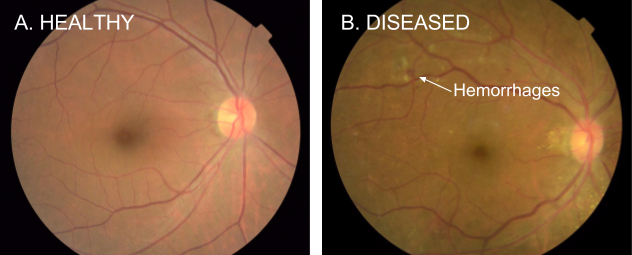
Figure 4: **Retinal Hemorrhages in DR Screening**: Side-by-side fundus images illustrate the subtle visual features an ML screening system must detect. Identifying localized microvascular lesions (such as the indicated hemorrhage) requires preserving fine spatial resolution through the vision pipeline and establishing strict input-quality validation to handle lighting and camera variations in clinical field deployments. Source: Google.

Initial research achieved expert-level performance in controlled settings. However, the journey to clinical deployment revealed how technical excellence must integrate with data quality challenges, infrastructure constraints in rural clinics, regulatory requirements, and workflow integration.⁹ For the metrics that recur in this case, sensitivity is the true-positive rate, specificity is the true-negative rate, and AUC is the area under the ROC curve. The same constraint propagation dynamics apply whether the target is medical imaging systems or mobile applications like MobileNetV2, and the lifecycle stages ahead trace these dynamics in concrete detail.

⁹ Healthcare AI deployment gap: In the Thai DR deployment studied by Beede et al. (2020), real clinics exposed workflow, image-quality, infrastructure, and human-factors constraints that were absent from controlled evaluation. The case shows why laboratory metrics alone do not establish deployment readiness.

Beede, Emma, Elizabeth Baylor, Fred Hersch, Anna Iurchenko, Lauren Wilcox, Paisan Ruamviboonsuk, and Laura M. Vardoulakis. 2020. “A Human-Centered Evaluation of a Deep Learning System Deployed in Clinics for the Detection of Diabetic Retinopathy.” Proceedings of the CHI Conference on Human Factors in Computing Systems (CHI), 1–12. https://doi.org/10.1145/3313831.3376718.

Stage interface specification

Each lifecycle stage operates as a distinct engineering phase with defined inputs, outputs, and quality invariants. Think of these as API contracts between teams. A microservice relies on an interface specification to make integration assumptions explicit; a data pipeline similarly relies on schema and distribution contracts to detect incompatibilities before they propagate. Table 3 formalizes these contracts, making explicit what each stage must receive and produce. This turns the abstract lifecycle diagram (figure 3) into actionable engineering requirements. When a stage’s output fails to meet its contract, the deficiency may propagate into dependent stages.

Table 3: Stage Interface Specification: Each lifecycle stage has explicit input requirements, output deliverables, and quality invariants that must hold for the stage to be considered complete. Violations of these contracts create technical debt that compounds through subsequent stages. The deployment paradigm selection in Problem Definition (Cloud, Edge, Mobile, or TinyML from ML Systems) constrains all downstream stages, as a TinyML target imposes different data, model, and monitoring requirements than a Cloud target.

Stage	Input Contract	Output Contract	Quality Invariant
Problem Definition	Business requirements; operational context	Measurable objectives; deployment paradigm selection; resource constraints	All success criteria are quantifiable; target deployment paradigm is explicit
Data Collection & Preparation	Objectives; deployment target; quality requirements	Versioned dataset with schema; preprocessing pipeline; data validation rules	Distribution approximates anticipated production environment; labeling meets accuracy requirements
Model Development & Training	Dataset; accuracy targets; resource constraints	Trained model weights; training configuration; experiment logs	Meets accuracy thresholds within computational budget; architecture compatible with deployment target
Evaluation & Validation	Trained model; held-out test data; evaluation criteria	Performance metrics across subgroups; failure mode analysis; validation certificate	No critical subgroup falls below minimum thresholds; confidence calibration meets domain requirements
Deployment & Integration	Validated model; infrastructure requirements; service-level agreement (SLA) targets	Serving endpoint; monitoring instrumentation; rollback procedures	Latency and throughput meet paradigm requirements; integration tests pass
Monitoring & Maintenance	Live system; performance baselines; alert threshold	Drift detection alerts; update-review criteria; incident reports	Alert coverage and detection windows are defined; detected degradation triggers review

This specification reveals why ML projects experience the iteration cycles diagrammed in figure 3. When a downstream stage discovers that an upstream contract was violated (for example, evaluation reveals the training data distribution does not match production), the project must iterate back to fix the root cause. Teams that validate contracts at each stage transition catch violations early, when correction costs are lowest. This validation process is best understood as auditing stage transitions.

Example 1.1: Auditing stage transitions

Scenario: An engineering team claims to have completed Problem Definition for a medical imaging classifier, attempting to transition to Data Collection without establishing deployment target constraints.

Diagnosis: The output contract lacks deployment paradigm selection and resource constraints (latency and memory targets). Attempting to deploy late in the lifecycle exposes violations (e.g., edge device memory limit < 200 MB), incurring 16× the cost compared to early correction.

Systems lesson: Stage transitions act as control-plane quality gates in the ML lifecycle. Enforcing strict output contract validation before proceeding downstream prevents expensive upstream rework and ensures data collection aligns with target deployment hardware.

The DR case study and Stage Interface Specification provide the concrete context and formal contracts that ground each lifecycle stage. The first stage, Problem Definition, records the constraints that subsequent stages must satisfy.

Self-Check: Question

Order the following lifecycle phases in the canonical sequence established in the chapter for a new ML system project: (1) Deployment and Integration, (2) Problem Definition, (3) Monitoring and Maintenance, (4) Data Collection and Preparation, (5) Model Development and Training, (6) Evaluation and Validation.
An engineering team completes Problem Definition with clinical sensitivity targets but marks the target deployment paradigm as ‘TBD — to be determined after model training.’ According to the Stage Interface Specification, what should the transition audit verdict be, and why?
1. A. Approved, because decoupling model development from hardware targets allows researchers to maximize accuracy before applying post-hoc pruning.
2. B. Approved with warning, provided the team commits to using cloud inference if the model exceeds edge memory budgets.
3. C. Blocked, because Problem Definition’s output contract explicitly requires deployment paradigm and resource constraints to be established before data collection and modeling begin.
4. D. Blocked only if the model architecture requires distributed multi-GPU training, since single-device models can adapt to any deployment target.
The chapter discusses MobileNetV2 with its ~600 MFLOPs inference budget as a lighthouse case study for workflow thinking. Explain how establishing this mobile constraint at Problem Definition propagates across Data Collection, Model Development, and Evaluation.
Which mapping between lifecycle stages and the terms in the Iron Law of ML Systems ( = + + L_{}$) is conceptually correct according to the chapter?
1. A. Problem Definition governs {}$; Evaluation governs $; Monitoring governs $\text{BW}$.
2. B. Data Collection sets {}$; Model Development sets $\text{BW}$; Deployment sets {}$.
3. C. Deployment governs $; Model Development governs {\text{vol}}$; Data Collection governs {}$.
4. D. Data Collection and Preparation shapes $ and {}$; Model Development and Training sets $; Deployment and Integration minimizes {\text{lat}}$.
To prevent defect propagation across lifecycle boundaries, the chapter formalizes each stage boundary using a(n) ____ contract, which defines required inputs, output deliverables, and non-negotiable quality invariants.

See Answers →

Problem Definition

Problem definition in ML begins with sentences that look deceptively simple. A product manager writes: “Build a model that detects diabetic retinopathy.” That single sentence conceals a dozen engineering decisions: sensitivity thresholds for patient safety, hardware capabilities in rural clinics, latency budgets that keep clinicians engaged, and regulatory frameworks governing approval. Some conventional requirements translate directly into implementation rules. In ML systems, defining what the system should do is inseparable from defining how it will learn to do it and the physical constraints under which it must operate. This first stage, the leftmost box in figure 3, lays the foundation for all subsequent phases in the ML lifecycle.

The DR screening case makes this concrete. What appears to be a straightforward classification task (detect disease in retinal photographs) actually requires balancing five competing constraints: diagnostic accuracy (patient safety), computational efficiency (rural clinic hardware), workflow integration (clinical adoption), regulatory compliance (FDA approval), and cost-effectiveness (sustainable deployment in resource-limited settings). Each constraint tightens the feasible design space for the others: pursuing higher accuracy through larger models conflicts with the hardware budget; achieving regulatory compliance demands annotation protocols that increase data collection costs. ML adds learned statistical behavior to a multi-constraint optimization problem that also appears in conventional systems.

Constraint layers

The DR example reveals that ML problem definitions are not single requirements but stacks of interacting constraint layers. Accuracy constraints (>90 percent sensitivity, >80 percent specificity across diverse populations and equipment) sit on top of infrastructure constraints (edge devices with limited compute, intermittent connectivity, inference within clinical workflow timeframes) which sit on top of regulatory constraints (FDA validation, audit trails, privacy compliance). Each layer narrows the feasible design space for the layers above it.

Privacy compliance in an ML system carries a distinctive operational weight that a generic data-handling rule does not capture. In a traditional database, deleting a patient’s record is a DELETE statement. In an ML system, model weights may encode statistical patterns learned from that record: where law or a regulator requires removing that influence, compliance may require machine unlearning (an active research area with incomplete guarantees) or retraining on the remaining data. The obligation and remedy depend on the governing rule and system; at DR-system scale, either can make privacy compliance a recurring compute-budget item and training provenance an architectural constraint.

This layered structure generalizes beyond healthcare. Any ML problem definition must address at least three constraint layers: statistical (what accuracy, across which subpopulations), physical (what hardware, under what latency and memory budgets), and operational (what regulatory, organizational, or workflow requirements apply). The constraint propagation principle (section 1.9.1) explains why: a constraint that exists but remains unspecified does not disappear—it may surface later after dependent decisions have hardened.

The specific constraints for the DR system did not emerge from technical analysis alone. They required systematic collaboration between engineers, ophthalmologists, and clinic administrators to translate clinical needs into measurable engineering requirements. Key decisions (balancing model complexity with hardware limitations, ensuring interpretability for healthcare providers, and accounting for patient privacy) emerged from this cross-disciplinary process. Without domain expertise, the engineering team might have optimized for aggregate accuracy while missing the sensitivity threshold that determines clinical safety.

War Story 1.1: When the label was the bias (2018)

Context: In 2014, Amazon assembled an engineering team at its Edinburgh hub to build an internal machine-learning system for ranking technical job applicants, training it on ten years of resumes submitted to Amazon (Dastin 2018).

Mechanism: Because prior hiring was male-dominated, the model learned that male-coded language correlated with hiring success, systematically penalizing terms like “women’s” and downgrading graduates of all-women’s colleges.

Impact: The model reproduced historical hiring bias, rendering automated resume screening unsuitable for production recruitment.

Fix: Amazon abandoned the experimental tool after attempts to remove explicit gender signals could not guarantee that it would not learn other discriminatory proxies.

Systems lesson: Problem definition must specify fairness, auditability, and rejection criteria before data collection and training. A workflow trained on biased labels does not learn the operational goal; it learns to reproduce the labels.

Dastin, Jeffrey. 2018. “Amazon Scraps Secret AI Recruiting Tool That Showed Bias Against Women.” Reuters.

Problem definitions evolve

ML problem definitions may evolve as a system scales. Suppose a DR program grows from a handful of clinics with consistent imaging setups to hundreds with varying equipment, staff expertise, and patient demographics.¹⁰ Such growth may require stratified accuracy targets, support for heterogeneous hardware, and revised reporting requirements.

¹⁰ Demographic drift: Population changes can expose performance gaps that aggregate evaluation obscures. Facial-analysis benchmarks found large demographic error-rate disparities (Buolamwini and Gebru 2018), while a healthcare risk-scoring study found racially biased allocation from a proxy label despite similar need (Obermeyer et al. 2019). These examples illustrate why a growing DR program should evaluate subgroup performance rather than claiming that such a rollout occurred.

Buolamwini, Joy, and Timnit Gebru. 2018. “Gender Shades: Intersectional Accuracy Disparities in Commercial Gender Classification.” Conference on Fairness, Accountability and Transparency, 77–91.

Obermeyer, Ziad, Brian Powers, Christine Vogeli, and Sendhil Mullainathan. 2019. “Dissecting Racial Bias in an Algorithm Used to Manage the Health of Populations.” Science 366 (6464): 447–53. https://doi.org/10.1126/science.aax2342.

This evolution is not a sign of poor initial planning—it is inherent to ML systems. Scaling exposes edge cases invisible at pilot scale, and production data reveals distributional properties that no training set fully captures. The problem definition must accommodate this reality by specifying both current targets and the mechanisms for revising them: which metrics trigger re-evaluation, who approves revised thresholds, and how changes propagate to downstream stages.

Self-Check: Question

Why does the statement ‘Build a computer vision model that detects diabetic retinopathy’ fail as a complete problem definition for an ML system?
1. A. It specifies only a high-level task while omitting the statistical constraint layers (sensitivity/specificity floors across subgroups), physical constraints (edge device memory/latency budgets), and operational constraints (regulatory compliance, clinical workflow integration).
2. B. It fails to specify which exact deep neural network backbone and learning rate schedule must be used during training.
3. C. It defines an image classification problem when medical AI systems must always be framed as unsupervised anomaly detection tasks.
4. D. It defines quantifiable objectives before data collection has occurred, which violates standard ML agile practices.
Explain why ophthalmologists and clinic administrators must participate directly in Problem Definition for a DR screening system, rather than being consulted only during clinical evaluation.
In the 2018 Amazon automated recruiting war story cited in the chapter, an ML model trained on ten years of resumes was abandoned because it systematically penalized female applicants. What fundamental systems lesson does this case illustrate regarding Problem Definition?
1. A. Resume screening models require recurrent neural networks rather than transformer architectures to avoid learning gendered proxies.
2. B. Offline evaluation metrics are inherently incapable of measuring demographic disparities in supervised learning models.
3. C. A model trained on historical data learns to reproduce historical label biases rather than the intended operational goal; fairness criteria and auditability must be explicitly defined at Problem Definition.
4. D. Multi-class classification algorithms should not be applied to human evaluation tasks where ground truth is subjective.
True or False: When a diabetic retinopathy screening deployment scales from a 3-clinic pilot to 200 clinics across diverse regions, the high-level clinical intent (detect referable retinopathy early) remains stable, but the specific engineering targets (subgroup sensitivity thresholds, device latency budgets, and camera-specific preprocessing rules) must evolve.

See Answers →

Data Collection

With objectives defined and constraints layered, the next practical task is identifying the data that can teach the model to meet these objectives. The constraints, metrics, and deployment targets from problem definition exist only on paper until a team acquires the data that will teach the model to satisfy them. This transition from defining goals to data collection marks a critical juncture where many projects fail. As the survey in section 1.1.1 established, practitioners often report data-related activities as their primary time sink. In iron law terms, this stage primarily determines dataset size and composition $(D)$, along with the byte volume $(D_{\text{vol}})$ that downstream stages must move. The deployment constraints established during problem definition now become data requirements: if the model must run on edge devices, the data pipeline must produce inputs compatible with edge preprocessing. If the model must achieve 90 percent sensitivity across diverse populations, the data must include sufficient examples from each population.

Data collection and preparation is not merely a preliminary step but often a major engineering activity. Data Engineering addresses data engineering as its core focus. For DR screening, the challenge is substantial: the data must be statistically diverse enough to train a model that generalizes across populations, operationally feasible to collect in resource-limited clinics, and annotated with enough clinical rigor to satisfy regulatory scrutiny.

Problem definition decisions shape data requirements in the DR example. The multi-dimensional success criteria established (accuracy across diverse populations, hardware efficiency, and regulatory compliance) demand a data collection strategy that goes beyond typical computer vision datasets. Not all data contributes equally to learning, either—Data Selection shows how selection can retain comparable performance with less compute when a dataset contains redundancy, provided the selected subset preserves the evidence the task requires.

The DR system requires on the order of $10^5$ retinal fundus photographs, each reviewed by multiple expert ophthalmologists. Expert consensus addresses the inherent subjectivity in medical diagnosis (two ophthalmologists may disagree on borderline cases) while establishing ground truth labels that can withstand regulatory scrutiny. The annotation process must capture clinically relevant features like microaneurysms, hemorrhages, and hard exudates across the full spectrum of disease severity.

Raw high-resolution retinal scans can reach tens of megabytes per image before compression, creating substantial infrastructure challenges. A clinic processing dozens of patients per day can produce gigabytes to tens of gigabytes of imaging data per week. This volume can occupy much of a limited uplink during clinic hours, making local processing one option alongside compression, batching, scheduling, or increased link capacity.

Edge summaries beat raw medical-image uploads when bandwidth dominates.

Napkin Math 1.2: Bandwidth vs. compute

Problem: A rural clinic captures retinal images for DR screening. How much of the assumed same-shift uplink window would raw uploads occupy, and what alternatives reduce that occupancy?

Math:

Daily data: At 150 patients/day, 10 photos/patient, and 5 MB/photo, the clinic produces 7.5 GB/day.
Upload time: The uplink is 2 Mb/s, or 0.25 MB/s. Dividing 7,500 MB by that rate gives 30,000 s, approximately 8.3 h.
Constraint: If the clinic requires same-shift upload during its 8 h operating window, this transfer alone occupies the link for 104.2 percent of that window and may contend with other traffic.

Systems insight: Local inference with uploaded detection summaries (10 KB/patient) reduces bandwidth usage by 5,000×. Overnight batching, compression, scheduling, or a faster link are alternatives not compared by this calculation.

Lab-to-field data gap

Laboratory data and production data inhabit different worlds. This lab-to-field gap appears when DR screening deploys to rural clinics across Thailand and India: images arrive from diverse camera equipment operated by staff with varying expertise, often under suboptimal lighting with inconsistent patient positioning. A model trained on high-quality research images from standardized fundus cameras may fail on blurry, poorly-lit images from older equipment—not because the algorithm is wrong, but because the data distribution has shifted beyond the training envelope.

As the Bandwidth vs. Compute exercise quantified, this data volume makes same-shift raw upload difficult under the scenario assumptions. The scenario therefore evaluates edge deployment using specialized hardware such as NVIDIA Jetson.¹¹ Local preprocessing reduces bandwidth requirements by orders of magnitude but demands correspondingly more local computation, forcing a trade-off: simpler models that run on constrained hardware, or more powerful edge devices that increase per-clinic costs.

¹¹ NVIDIA Jetson: NVIDIA’s Jetson family spans a wide SKU spectrum, from Jetson Orin Nano (7–15 W) through Jetson Orin NX (10–25 W) to Jetson AGX Orin (15–60 W). This scenario uses an Orin Nano-class device (4–8 GB shared LPDDR5, 7–15 W power envelope) as a concrete edge target. Its memory and power budgets constrain model complexity, while selecting a larger device changes both the feasible model and the per-clinic cost.

The bandwidth constraint makes infrastructure a data-collection decision rather than a late implementation detail. The scenario architecture combines edge devices for local inference and preprocessing, clinic aggregation servers for data management and buffering, and cloud training infrastructure for periodic model updates. It targets end-to-end latency under 100 milliseconds and operation without connectivity-induced delays.

Privacy constraints impose a similar architectural decision. Patient privacy regulations may motivate local retention or distributed training, but they generally specify protections and permitted uses rather than one required training topology. Workflows that keep raw clinic data local while sharing only approved updates or summaries add complexity to both data collection and model training infrastructure.

Distributed data infrastructure

If a deployment grows from a handful of clinics to hundreds, data infrastructure must scale accordingly. Each retinal image travels through multiple stages: clinic cameras capture the image, local systems provide initial storage and processing, quality validation checks ensure usability, secure transmission moves data to central systems, and finally, integration with training datasets completes the pipeline. The infrastructure decisions at each stage are shaped by the deployment constraints established during problem definition.

Storage tiers are another place where the data pipeline either preserves or erodes downstream iteration velocity. Different data access patterns demand different storage solutions, so teams typically implement tiered storage architectures,¹² each calibrated to access frequency and performance requirements.

¹² Tiered storage: Places data on different storage media based on access frequency and performance requirements. The storage price gap is roughly 4.3× in this example: Non-Volatile Memory Express (NVMe) SSDs deliver 500,000+ input/output operations per second (IOPS) at ~$0.10/GB/month, while object storage costs ~$0.023/GB/month but with 100–200 ms latency. For ML training loops requiring sustained sequential reads at 1–10 GB/s, choosing the wrong tier converts a compute-bound training pipeline into an I/O-bound one, directly inflating the iron law’s data term $(D_{\text{vol}}/\text{BW})$.

Hot storage uses high-throughput NVMe SSDs for data currently used in training loops. Warm storage uses S3-compatible object storage for recent datasets and active validation sets. Cold storage uses low-cost archival systems, such as AWS Glacier, for historical data required for regulatory audit trails but rarely accessed.

In practice, the boundary between tiers is dynamic: a dataset migrates from warm to hot when selected for the next training run, and from hot to cold when the model it trained is superseded. Automated lifecycle policies manage these transitions, promoting data based on training schedules and demoting it based on access recency—a pattern that Data Engineering explores in detail.

Rural clinic deployments face severe connectivity constraints that force a choice between transmission strategies. Clinics with reliable broadband can stream images in near-real-time for centralized processing, but clinics with intermittent satellite links, common in remote regions of India and sub-Saharan Africa, require store-and-forward architectures that batch images during connectivity windows and reconcile results asynchronously. The choice propagates through the entire stack: store-and-forward clinics need larger local storage buffers, more robust local inference capabilities, and conflict-resolution logic when locally generated predictions differ from later cloud-based analysis.

Infrastructure scalability poses a harder challenge than raw capacity. As the system grows from a handful of pilot clinics to hundreds of production sites, data heterogeneity grows alongside data volume: each clinic’s camera model, lighting environment, and operator habits can produce a different image distribution. The infrastructure must handle increasing throughput while also tracking which data came from where. This provenance metadata proves essential for debugging accuracy regressions at specific sites and for satisfying the audit trail requirements that regulatory validation demands. Scaling from initial clinics to a broader network therefore introduces emergent complexity: variability in equipment, workflows, operating conditions, and image sizes as newer clinics add higher-resolution devices. Each clinic becomes a distinct data source,¹³ yet the system must evaluate performance across the full network.

¹³ Distributed clinic data: Training across clinic sites without simply pooling all raw data addresses privacy and governance constraints, but it shifts cost into coordination. Each site may use different cameras, serve different patient populations, and follow different operating routines, so the system must track where data came from and how each site differs. The workflow cost is therefore not just storage capacity; it is the engineering work needed to compare, validate, and update models across sites whose data does not behave identically.

The workflow response is coordination infrastructure. Shared artifact repositories, versioned APIs, and automated testing pipelines make clinic-specific variation visible before it becomes a model failure. That same heterogeneity is what makes point-of-capture validation necessary: the larger and more varied the clinic network becomes, the less useful it is to discover quality failures weeks later in a centralized training run.

Quality assurance and validation

A blurry retinal image that slips past quality checks does not merely waste storage. If such images enter training with unreliable labels or appear frequently in production, they can distort the evidence available to the model and increase error risk. Quality assurance ensures that data meets the requirements downstream stages depend on. In our DR example, automated checks at the point of collection flag issues like poor focus or incorrect framing, allowing clinic staff to recapture images immediately rather than discovering the problem weeks later during model training.

Validation extends beyond image quality to verify proper labeling, patient association, and privacy compliance. Local validation catches problems at the point of capture; centralized validation detects distributional anomalies across the full clinic network—for instance, flagging when a particular site’s images skew toward a narrow demographic range that would bias the training set.

Data collection decisions directly constrain model development: bandwidth limits dictate what architectures are feasible, privacy requirements shape training pipelines, and quality variations across clinic environments determine robustness requirements. Figure 5 traces these feedback pathways concretely. Follow each labeled arrow: evaluation reveals the DR model underperforms on images from older fundus cameras, triggering targeted data collection from clinics using that equipment. Validation across diverse patient populations shows lower sensitivity for patients with cataracts, driving data augmentation strategies that simulate lens opacities. Monitoring detects accuracy drift in clinics that upgraded their imaging equipment, feeding back to update preprocessing steps.

\begin{tikzpicture}[line join=round,font=\sffamily\small]
\tikzset{%
  Box/.style={align=flush center,
    inner xsep=2pt,
    node distance=0.65,
    draw=GreenLine,
    line width=0.75pt,
    fill=mygreen!06,
    %text width=35mm,
    minimum width=37mm, minimum height=16mm
  },
  Box2/.style={Box, draw=BrownLine, fill=BrownL!30,
  },
  Txt/.style={font=\sffamily\footnotesize,text=black!90
  },
  LineA/.style={black!30,line width=1.5pt,{-{Triangle[width=1.0*5pt,length=9pt]}},shorten <=2pt,shorten >=2pt},
}

%funnel
\tikzset{%
 pics/funnel/.style = {
        code = {
        \pgfkeys{/channel/.cd, #1}
\begin{scope}[local bounding box=FUNNEL,scale=\scalefac, every node/.append style={transform shape}]
\draw[fill=\filllcolor!50,line width=\Linewidth,draw=\drawcolor](-0.12,-0.81)--(-0.19,-0.25)--(-0.7,0.41)--(0.7,0.41)--(0.19,-0.25)--(0.12,-0.81)--cycle;
\draw[fill=\filllcolor!50,line width=\Linewidth,draw=\drawcolor](-0.19,-0.25)--(0.08,-0.25);
\draw[fill=\filllcolor!50,line width=\Linewidth,draw=\drawcolor](0.16,-0.09)--(0.41,0.31);
%
\node[line width=\Linewidth,draw=\drawcolor,fill=\filllcolor!50,inner sep=1pt,
rectangle,rounded corners=2pt,minimum width=16mm,minimum height=5pt]at(0,0.5){};
%
\foreach \i in{-0.5,0,0.5}{
\node[single arrow, line width=0.8*\Linewidth,draw=\filllcirclecolor,fill=\filllcirclecolor, rotate=270,inner sep=1pt,
      minimum width =9pt, single arrow head extend=2pt,
      minimum height=5mm]at(\i,0.9) {}; % length of arrow
   }
\node[single arrow,line width=0.8*\Linewidth,draw=\filllcirclecolor,fill=\filllcirclecolor, rotate=270,inner sep=1pt,
      minimum width =11pt, single arrow head extend=2pt,
      minimum height=5mm]at(0,-1.1) {}; % length of arrow
 \end{scope}
     }
  }
}
%nodes
\tikzset{
pics/nodes/.style = {
        code = {
        \pgfkeys{/channel/.cd, #1}
\begin{scope}[shift={($(0,0)+(0,0)$)},scale=\scalefac,every node/.append style={transform shape}]
\foreach \x/\y[count=\a] in {-0.2/0.35,
0.7/0.6,-0.5/1.4,-1.20/-0.8,-0.1/-1.3,-0.4/-0.43,
0.61/-0.3,1/-0.85,0.45/1.2,-0.96/0.63}{
\node[circle,fill=myblue,draw=black,inner sep=0pt,minimum size=3mm](XB\a)at(\x,\y){};
}
\foreach \x/\y[count=\a] in {-2.0/0.1
}{
\node[circle,fill=myred,draw=black,inner sep=0pt,minimum size=3mm](XR\a)at(\x,\y){};
}

\foreach \x/\y[count=\a] in {1.87/0.1
}{
\node[circle,fill=mygreen,draw=black,inner sep=0pt,minimum size=3mm](XG\a)at(\x,\y){};
}

\foreach \x in {1,3,4,6,10}{
\draw[RedLine,line width=0.5pt](XR1) edge  (XB\x);
}
\foreach \x in {1,2,5,8,9}{
\draw[mygreen,line width=0.5pt](XG1) edge  (XB\x);
}
\foreach \x in {2,3,6,9,10}{
\draw[black,line width=0.5pt](XB1) edge  (XB\x);
}
\foreach \x in {4,5,7}{
\draw[black,line width=0.5pt](XB6) edge  (XB\x);
}
\draw[black,line width=0.5pt](XB4) edge  (XB5);
\draw[black,line width=0.5pt](XB3) edge  (XB9);
\foreach \x in {2,8}{
\draw[black,line width=0.5pt](XB7) edge  (XB\x);
}
\end{scope}
    }
  }
}
%testing
\tikzset{
pics/testing/.style = {
        code = {
        \pgfkeys{/channel/.cd, #1}
\begin{scope}[local bounding box=TESTING1,shift={($(0,0)+(0,0)$)},scale=\scalefac,every node/.append style={transform shape}]
\newcommand{\tikzxmark}{%
\tikz[scale=0.18] {
    \draw[line width=0.7,line cap=round,RedLine] (0,0) to [bend left=6] (1,1);
    \draw[line width=0.7,line cap=round,RedLine] (0.2,0.95) to [bend right=3] (0.8,0.05);
}}
\newcommand{\tikzxcheck}{%
\tikz[scale=0.16] {
    \draw[line width=0.7,line cap=round,GreenLine] (0.5,0.75)--(0.85,-0.1) to [bend left=16] (1.5,1.55);

}}
 \node[minimum width  =15mm, minimum height = 20mm, inner sep = 0pt,
        rounded corners=2pt,draw = \drawcolor, fill=\filllcolor!10, line width=\Linewidth](COM){};
 \node[minimum width  =8mm, minimum height = 2mm, inner sep = 0pt,anchor=north,
        rounded corners=1.5pt,draw =white, fill=\drawcolor!70, line width=0.7*\Linewidth]at
        ($(COM.north)+(0,0.75mm)$)(GOR){};
 \node[minimum size = 2.5mm, inner sep = 0pt,circle,%anchor=north,
        rounded corners=0.5pt,draw =white, fill=\drawcolor!70, line width=0.7*\Linewidth]at(GOR.north)(GOR1){};
\node[draw=GreenLine,inner sep=4pt,fill=white](CB1) at ($(COM.north west)!0.25!(COM.south west)+(0.3,0)$){};
\node[xshift=0pt]at(CB1){\tikzxcheck};
\node[draw=RedLine,inner sep=4pt,fill=white](CB2) at ($(COM.north west)!0.5!(COM.south west)+(0.3,0)$){};
\node[xshift=0pt]at(CB2){\tikzxmark};
\node[draw=RedLine,inner sep=4pt,fill=white](CB3) at ($(COM.north west)!0.75!(COM.south west)+(0.3,0)$){};
\node[xshift=0pt]at(CB3){\tikzxmark};
\draw[GreenLine,decoration={zigzag,segment length=4pt, amplitude=0.5pt},decorate]($(CB1)+(0.3,0.05)$)--++(0:0.8);
\draw[GreenLine,decoration={zigzag,segment length=4pt, amplitude=0.5pt},decorate]($(CB1)+(0.3,-0.12)$)--++(0:0.7);
\draw[RedLine,decoration={zigzag,segment length=4pt, amplitude=0.5pt},decorate]($(CB2)+(0.3,0.05)$)--++(0:0.8);
\draw[RedLine,decoration={zigzag,segment length=4pt, amplitude=0.5pt},decorate]($(CB2)+(0.3,-0.12)$)--++(0:0.6);
\draw[RedLine,decoration={zigzag,segment length=4pt, amplitude=0.5pt},decorate]($(CB3)+(0.3,0.05)$)--++(0:0.8);
\draw[RedLine,decoration={zigzag,segment length=4pt, amplitude=0.5pt},decorate]($(CB3)+(0.3,-0.12)$)--++(0:0.6);
\end{scope}
    }
  }
}
%check mark
\tikzset{pics/.cd,
checkmark/.style={code={
        \pgfkeys{/channel/.cd, #1}
\pgfgettransformentries{\tmpxx}{\tmp}{\tmp}{\tmp}{\tmp}{\tmp}
\draw[line width=\tmpxx*1pt,draw=none,fill=\filllcirclecolor,line join=bevel] (0,.35) -- (.25,0) to[bend left=5] (0.8,.6) to[bend
right=5] (.25,.18) -- cycle;}}}
\tikzset{%
 pics/checkI/.style = {
        code = {
        \pgfkeys{/channel/.cd, #1}
\begin{scope}[local bounding box=CHECK,scale=\scalefac, every node/.append style={transform shape}]
\node[fill=\filllcolor,minimum width=6mm, minimum height=6mm,
            outer sep=2pt] (C1) {};
\pic[shift={(-0.27,-0.19)},scale=0.7]{checkmark};
 \end{scope}
     }
  }
}
%cloud
\tikzset {
pics/cloudA/.style = {
        code = {
        \pgfkeys{/channel/.cd, #1}
\begin{scope}[local bounding box=CLO,scale=\scalefac,, every node/.append style={transform shape}]
\node[draw=\drawcolor!90!red,line width=\Linewidth,minimum width=6mm,minimum height=12mm](VSK)at(0,0.5){};
\node[draw=\drawcolor!90!red,line width=\Linewidth,fill=white,minimum width=9mm,minimum height=4mm](VSKG)at(VSK.north){};
\node[draw=\drawcolor!90!red,line width=\Linewidth,fill=white,minimum width=9mm,minimum height=4mm](VSKC)at(VSK.center){};
\node[draw=\drawcolor!90!red,line width=\Linewidth,fill=white,minimum width=9mm,minimum height=4mm](VSKD)at(VSK.south){};
\draw[fill=\filllcolor,draw=\drawcolor!60,,line width=\Linewidth](0,0)to[out=170,in=180,distance=11](0.1,0.61)
to[out=90,in=105,distance=17](1.07,0.71)
to[out=20,in=75,distance=7](1.48,0.36)
to[out=350,in=0,distance=7](1.48,0)--(0,0);
\draw[draw=\drawcolor!60,,line width=\Linewidth](0.27,0.71)to[bend left=25](0.49,0.96);
\draw[draw=\drawcolor!60,,line width=\Linewidth](0.67,1.21)to[out=55,in=90,distance=13](1.5,0.96)
to[out=360,in=30,distance=9](1.68,0.42);
\node[single arrow, draw=orange,fill=orange,
      minimum width = 10pt, single arrow head extend=3pt,
      minimum height=10mm,
      rotate=270]at(1.05,0) {};
\end{scope}
}
}
}
%data
\tikzset{mycylinder/.style={cylinder, shape border rotate=90, aspect=1.3, draw, fill=white,
minimum width=25mm,minimum height=11mm,line width=\Linewidth,node distance=-0.15},
pics/data/.style = {
        code = {
        \pgfkeys{/channel/.cd, #1}
\begin{scope}[local bounding box=STREAMING,scale=\scalefac, every node/.append style={transform shape}]
\node[mycylinder,fill=\filllcolor!50] (A) {};
\node[mycylinder, above=of A,fill=\filllcolor!30] (B) {};
\node[mycylinder, above=of B,fill=\filllcolor!10] (C) {};
\fill[\filllcolor!50!black]($(C.west)!0.12!(C.east)$)circle(3pt);
\fill[\filllcolor!50!black]($(B.west)!0.12!(B.east)$)circle(3pt);
\fill[\filllcolor!50!black]($(A.west)!0.12!(A.east)$)circle(3pt);
 \end{scope}
     }
  }
}
%display
\tikzset{%
    comp/.style = {draw,
        minimum width  =18mm,
        minimum height = 15mm,
        inner sep      = 0pt,
        rounded corners=3pt,
       draw = \drawcolor,
       fill=\filllcolor!10,
       line width=2.0pt
    },
 pics/displayK/.style = {
        code = {
        \pgfkeys{/channel/.cd, #1}
\begin{scope}[local bounding box=COMPUTER1,scale=\scalefac, every node/.append style={transform shape}]
\node[comp](\picname-COM){};
\draw[draw = \drawcolor,line width=\Linewidth]($(\picname-COM.south west)!0.4!(\picname-COM.south east)$)--++(270:0.2)coordinate(DL);
\draw[draw = \drawcolor,line width=\Linewidth]($(\picname-COM.south west)!0.6!(\picname-COM.south east)$)--++(270:0.2)coordinate(DD);
\draw[draw = \drawcolor,line width=3*\Linewidth,shorten <=-3mm,shorten >=-3mm](DL)--(DD);
 \draw[
  line width=1pt,
  draw=red,
  line cap=round,
  line join=round
](-0.70,0) --(-0.40,0) --(-0.30,0.13) --(-0.2,-0.18) --(-0.05,0.32) --(0.05,-0.15) --
(0.15,0.23) --(0.38,-0.15) --(0.40,0.0) --(0.70,0.0);
\end{scope}
   }
  }
}

\pgfkeys{
  /channel/.cd,
   Depth/.store in=\Depth,
  Height/.store in=\Height,
  Width/.store in=\Width,
  filllcirclecolor/.store in=\filllcirclecolor,
  filllcolor/.store in=\filllcolor,
  drawcolor/.store in=\drawcolor,
  drawcircle/.store in=\drawcircle,
  scalefac/.store in=\scalefac,
  Linewidth/.store in=\Linewidth,
  picname/.store in=\picname,
  filllcolor=BrownLine,
  filllcirclecolor=violet!20,
  drawcolor=red,
  drawcircle=violet,
  scalefac=1,
  Linewidth=0.5pt,
  Depth=0.2,
  Height=0.5,
  Width=0.25,
  picname=C
}
% Model Training
\node[Box](B1){};
\coordinate(GO1)at($(B1.north west)!0.38!(B1.north east)$);
\coordinate(T1)at($(GO1)!0.5!(B1.south east)$);
\coordinate(I1)at($(B1.west)!0.21!(B1.east)$);
\node[align=center]at(T1){Model\\ Training};
\node[Box,fill=none]{};
\pic[shift={(0.2,0)}] at  (I1){nodes={scalefac=0.4,picname=1,drawcolor=orange,filllcirclecolor=orange!20,filllcolor=orange}};
%Model Deployment
\node[Box,right=5of B1](B2){};
\coordinate(GO2)at($(B2.north west)!0.4!(B2.north east)$);
\coordinate(T2)at($(GO2)!0.5!(B2.south east)$);
\coordinate(I2)at($(B2.west)!0.24!(B2.east)$);
\node[align=center]at(T2){Model\\ Deployment};
\pic[shift={(-0.36,-0.30)}] at  (I2){cloudA={scalefac=0.6,filllcirclecolor=orange!80,drawcolor=BlueLine,
filllcolor=cyan!10,  Linewidth=1.0pt}};
%Data Preparation
\node[Box,below left=0.5 of B1](B3){};
\coordinate(GO3)at($(B3.north west)!0.4!(B3.north east)$);
\coordinate(T3)at($(GO3)!0.5!(B3.south east)$);
\coordinate(I3)at($(B3.west)!0.24!(B3.east)$);
\node[align=center]at(T3){Data\\ Preparation};
\node[Box,below left=0.5 of B1,fill=none]{};
\pic[shift={(0,0.04)}] at  (I3){funnel={scalefac=0.55,Linewidth=0.5pt,
 filllcolor=mypurple,drawcolor=black,filllcirclecolor=red}};
%Model Evaluation
\node[Box,right=5 of B3](B4){};
\coordinate(GO4)at($(B4.north west)!0.4!(B4.north east)$);
\coordinate(T4)at($(GO4)!0.5!(B4.south east)$);
\coordinate(I4)at($(B4.west)!0.24!(B4.east)$);
\node[align=center]at(T4){Model\\ Evaluation};
\node[Box,right=5 of B3,fill=none]{};
\pic[shift={(-0.1,-0.02)}] at  (I4){testing={scalefac=0.6,drawcolor=mybrown,filllcolor=gray, Linewidth=1.0pt}};
\pic[shift={(0.3,-0.46)}] at  (I4){checkI={scalefac=0.7,filllcolor=GreenLine, filllcirclecolor=white,Linewidth=0.7pt}};
%Monitoring \& Maintenance
\node[Box,right=3.5 of B4](B5){};
\coordinate(GO5)at($(B5.north west)!0.4!(B5.north east)$);
\coordinate(T5)at($(GO5)!0.5!(B5.south east)$);
\coordinate(I5)at($(B5.west)!0.24!(B5.east)$);
\node[align=center]at(T5){Monitoring \&\\ Maintenance};
\node[Box,right=3.5 of B4,fill=none]{};
\pic[shift={(-0.02,0.06)}] at  (I5){displayK={scalefac=0.65,picname=D,
filllcolor=myblue, drawcolor=myblue,Linewidth=0.7pt}};
%Data Collection
\node[Box,below =1 of B3](B6){};
\coordinate(GO6)at($(B6.north west)!0.4!(B6.north east)$);
\coordinate(T6)at($(GO6)!0.5!(B6.south east)$);
\coordinate(I6)at($(B6.west)!0.24!(B6.east)$);
\node[align=center]at(T6){Data\\ Collection};
\node[Box,below =1 of B3,fill=none]{};
\pic[shift={(0,-0.5)}] at  (I6){data={scalefac=0.45,picname=1,filllcolor=red, Linewidth=0.6pt}};
%arrows
\draw[LineA](B6)--(B3);
\draw[LineA](B4)-|(B2);
\draw[LineA](B1.350)-|(B4);
\draw[LineA](B2)-|(B5.130);
\draw[LineA](B3.60)|-(B1);
\draw[LineA](B5.south)|-node[Txt,above,pos=0.6]{Performance Insights}(B6.350);
\draw[LineA](B4.south)|-node[Txt,above,pos=0.75]{Data gaps}(B6.10);
\draw[LineA](B4.west)-|node[Txt,above,pos=0.25]{Validation Issues}(B1);
\draw[LineA](B2.170)--node[Txt,above,pos=0.5]{Deployment Constraints}(B1.10);
%
\draw[LineA](B5)--++(0,35mm)-|node[Txt,above,pos=0.25]{Model Updates}(B1);
\draw[LineA](B5.50)--++(0,35mm)-|node[Txt,above,pos=0.25]{Data Quality Issues}(B3.120);
\end{tikzpicture}

Figure 5: Feedback Paths Across Lifecycle Stages: Multi-stage feedback pathways show how downstream discoveries can require upstream corrections. Data-quality and distribution gaps detected during evaluation may prompt targeted collection or augmentation, while operational constraints and performance drift can motivate model, data, or pipeline changes after investigation.

These feedback pathways reinforce a central point: data collection does not end when training begins. The quality, volume, and diversity of the data flowing through these pipelines now become the raw material for the next stage—turning curated datasets into trained models.

Self-Check: Question

A rural clinic captures 150 patients per day for DR screening, with 10 retinal photos per patient at 5 MB per photo. The clinic operates on an 8-hour daily shift with a 2 Mbps uplink. According to the chapter’s Bandwidth vs. Compute analysis, what operational bottleneck arises, and how does edge inference resolve it?
1. A. Daily raw image upload requires ~2.5 hours, which fits comfortably within the 8-hour window without needing edge processing.
2. B. Daily raw image upload generates 7.5 GB of data requiring ~8.3 hours to transfer—saturating the entire 8-hour clinic shift—whereas edge inference uploading 10 KB detection summaries reduces network traffic by roughly 5,000$\times$.
3. C. Daily raw image upload generates 75 GB of data, which exceeds daily satellite uplink capacity by a factor of 100$\times$ regardless of compression.
4. D. Raw uploads complete in 45 minutes, but cloud GPU queuing delay adds 12 hours of fixed inference latency.
Explain why a DR screening model achieving an AUC of 0.99 on a curated laboratory research dataset can experience a severe drop in sensitivity (e.g., falling to 78 percent) when deployed to rural clinics across Thailand and India.
In tiered storage architectures for ML pipelines, placing active training data in cold or warm object storage (e.g., S3 Standard with 100–200 ms latency) instead of local high-throughput NVMe SSDs directly degrades training performance by affecting which term in the Iron Law of ML Systems?
1. A. It increases the Operations ($) term by forcing the model to compute extra gradient updates.
2. B. It decreases peak hardware performance ({}$) by downclocking GPU compute cores.
3. C. It decreases hardware utilization efficiency ($\eta_{\text{hw}}$) solely through floating-point precision mismatches.
4. D. It inflates the data movement time ($\frac{D_{\text{vol}}}{\text{BW}}$), converting a compute-bound training pipeline into an I/O-bound stall where accelerators sit idle waiting for data batches.
True or False: In large-scale medical data collection, if collected images pass basic file format and schema validation, image-quality defects (such as blur, low contrast, or partial occlusion) can be safely ignored because deep neural networks naturally learn to filter out bad samples when trained on sufficiently large datasets.
In rural clinics with intermittent connectivity, an architecture that buffers captured images locally and reconciles inference results asynchronously with the central cloud during available network windows is known as a(n) ____ architecture.

See Answers →

Model Development

The DR team has 128,000 labeled retinal images, a validated preprocessing pipeline, and a target: more than 90 percent sensitivity on edge hardware with less than 50 ms inference latency. The question is no longer what data to collect but what model to build—and that question has no answer independent of the deployment constraints already established. In iron law terms, this stage defines the Operations $(O)$ term: architectural choices set the computational floor that hardware must sustain. The challenges extend well beyond selecting algorithms and tuning hyperparameters.¹⁴ Model Training covers the training methodologies, infrastructure requirements, and distributed training strategies in detail. In high-stakes domains like healthcare, every design decision affects clinical outcomes, so technical performance and operational constraints must be integrated from the start.

¹⁴ Hyperparameter: Architectural and optimizer choices (for example, learning rate and network depth) affect the computational work of training. A naive Cartesian grid that trains every combination independently incurs a multiplicative search cost: 5 hyperparameters with 4 values each produces 1,024 ($4^{5}$) configurations. Early stopping, multifidelity methods, and adaptive search can avoid completing every run, which is why the grid represents a baseline rather than an unavoidable cost.

¹⁵ Transfer learning: For the same architecture, transfer learning changes how parameters are initialized and optimized, not the operations required at inference.

Russakovsky, Olga, Jia Deng, Hao Su, Jonathan Krause, Sanjeev Satheesh, Sean Ma, Zhiheng Huang, et al. 2015. “ImageNet Large Scale Visual Recognition Challenge.” International Journal of Computer Vision 115 (3): 211–52. https://doi.org/10.1007/s11263-015-0816-y.

Yosinski, Jason, Jeff Clune, Yoshua Bengio, and Hod Lipson. 2014. “How Transferable Are Features in Deep Neural Networks?” Advances in Neural Information Processing Systems 27.

The DR system faces a sharp training challenge: achieve expert-level diagnostic accuracy with finite labeled-data and optimization budgets. Transfer learning¹⁵ addresses this constraint by adapting a model pretrained on a source task to a target task. The ImageNet Large Scale Visual Recognition Challenge (ILSVRC) 2012 training subset contains 1.3 million labeled images (Russakovsky et al. 2015). Reusing learned representations can improve target-task optimization and generalization relative to random initialization, with the benefit depending on source-target similarity, which layers are transferred, and transfer-related optimization effects (Yosinski et al. 2014).

In the controlled validation study reported by Gulshan et al. (2016), transfer learning and a labeled dataset of 128,000 images produced an AUC¹⁶ of 0.99, with sensitivity of 97.5 percent and specificity of 93.4 percent at one operating point. The result demonstrates the potential of large-scale pretraining with domain-specific fine-tuning under the study conditions; it does not by itself establish deployment performance. The training strategy uses error gradients to adjust model weights; Neural Computation establishes that mechanism before Model Training develops the training systems around it.

Gulshan, Varun, Lily Peng, Marc Coram, Martin C. Stumpe, Derek Wu, Arunachalam Narayanaswamy, Subhashini Venugopalan, et al. 2016. “Development and Validation of a Deep Learning Algorithm for Detection of Diabetic Retinopathy in Retinal Fundus Photographs.” JAMA 316 (22): 2402. https://doi.org/10.1001/jama.2016.17216.

¹⁶ AUC (area under the ROC curve): Measures the area under the receiver operating characteristic (ROC) curve plotting true positive rate vs. false positive rate across all classification thresholds, ranging from 0 to 1; 0.5 represents random discrimination, and values below 0.5 are possible. Unlike accuracy, AUC is threshold-independent and insensitive to class prevalence, making it a common metric for medical screening systems. The systems consequence: a model with 0.99 AUC can still produce unacceptable sensitivity at the specific operating threshold chosen for deployment, so AUC alone cannot validate deployment readiness.

Achieving high accuracy is only the first challenge. Edge deployment constraints impose strict efficiency requirements: models may need to fit within tens to hundreds of megabytes, complete inference in tens of milliseconds, and operate within tight memory budgets.

From a workflow perspective, accuracy gains must always be weighed against deployment feasibility. Ensemble learning¹⁷ illustrates this trade-off: combining predictions from multiple models often yields better performance than any individual model, but adds inference work and memory usage. Bagging trains multiple models on different data subsets, boosting sequentially trains models to correct previous errors, and stacking uses a meta-model to combine base model predictions. These methods generate diversity in different ways, but every constituent model adds serving work that must fit the deployment budget. The Netflix Prize illustrates how ensemble complexity can impede production deployment.¹⁸

¹⁷ Ensemble learning: Combines predictions from multiple models (bagging, boosting, stacking). Inference compute and model storage generally sum across constituents. Serial execution can increase latency, while parallel execution trades latency for additional hardware and coordination; no fixed proportional latency multiplier follows from ensemble size.

¹⁸ Competition-production gap: The Netflix Prize winner used a complex ensemble, but Netflix did not deploy the winning approach because the additional accuracy did not justify the engineering effort (Johnston 2012).

Johnston, Casey. 2012. “Netflix Never Used Its $1 Million Algorithm Due to Engineering Costs.” Ars Technica, April.

Initial research models are often much larger (sometimes multiple gigabytes when using ensembles) and therefore violate deployment constraints, requiring systematic optimization to reach a deployable form factor while preserving clinical utility. These constraints drive systematic model compression and optimization rather than isolated accuracy tuning. Later model-compression techniques reduce computation and memory footprint, but each reduction must be revalidated against clinical accuracy. Model Compression details those techniques. The development process requires continuous iteration between accuracy optimization and efficiency optimization: model capacity, preprocessing choices, and execution cost all affect both dimensions simultaneously.

Reproducible system artifacts

The accuracy-efficiency balancing act produces more than trained weights alone. A common failure mode is treating the trained model weights as the sole output of this stage. In a mature ML workflow, the deliverable is a reproducible system artifact with four components:

Model Weights: The learned parameters.
Inference Code: The exact code used to run the model, including preprocessing logic.
Environment Specification: The complete dependency graph (for example, Docker container, requirements.txt, CUDA drivers) required to execute the code.
Configuration: Hyperparameters and runtime settings.

Without bundling the environment with the model, dependency mismatches can create dangerous failures. Some incompatibilities, including unsupported CUDA combinations or missing libraries, fail loudly and immediately. Other differences in compatible kernels, linear algebra libraries, or image-resizing routines such as OpenCV and PIL may alter floating-point results or pixel interpolation without crashing the serving process. These changes can shift model outputs and affect accuracy. Environment reproducibility is therefore necessary not only for successful execution but also for validating equivalent inference behavior. A model that achieves 99 percent accuracy in development must be reevaluated if its production environment changes, even when inference completes without an exception.

Accuracy vs. efficiency

Medical applications demand specific performance metrics¹⁹ that differ from the standard classification outputs and losses Neural Computation introduces. A DR system requires high sensitivity (to limit missed referable disease) and high specificity (to avoid overwhelming referral systems). These metrics must be maintained across diverse patient populations and image quality conditions.

¹⁹ Medical AI performance metrics: Medical AI evaluation emphasizes sensitivity (true positive rate) and specificity (true negative rate) alongside aggregate accuracy. This DR scenario sets a >90 percent sensitivity target because missed referable disease can delay care and contribute to avoidable vision loss; actual acceptance criteria are product- and regulator-specific. The subtler systems trap is positive predictive value (PPV): even a high-accuracy model can have low PPV in a low-prevalence population. This prevalence dependence can require different operating thresholds across deployment sites, a constraint invisible in standard ML evaluation.

²⁰ Model compression pipeline: Bridging the gap between research accuracy and edge deployment requires an iterative “compress-validate-adjust” loop. Each compression step can reduce model size or execution cost, but it can also silently degrade sensitivity below the clinical threshold. Finding a model that fits in device memory while preserving clinical sensitivity typically requires multiple iterations because only the full validation suite reveals whether the smaller model still satisfies the problem definition.

Optimizing for clinical performance alone is not enough. In this scenario, the model artifact must remain below 500 MB so that it fits comfortably within the edge target’s 4–8 GB of shared system memory, while the device operates inside a sub-20 watt power envelope and meets the clinical latency budget. Improvements in one dimension often come at the cost of others: the Operations $(O)$ term, the model byte footprint that contributes to $D_{\text{vol}}$, and fixed serving overhead $(L_{\text{lat}})$ can pull in different directions. Network Architectures explores model capacity, while ML Systems discusses deployment feasibility, and the inherent tension between them drives architectural decisions. Systematic compression and revalidation²⁰ can bridge the gap, meeting deployment requirements while aiming to preserve clinical utility.

The ensemble trade-off illustrates a broader pattern: choosing an ensemble of lightweight models over a single large model reduces per-model complexity (enabling edge deployment) but increases pipeline complexity (requiring orchestration logic and multi-model monitoring). Every architectural decision creates this kind of downstream ripple.

Constraint-driven development

Real-world constraints shape model development from initial exploration through final optimization, demanding systematic experimentation. Development begins when data scientists collaborate with domain experts (ophthalmologists in the DR case) to identify subtle lesions and image-quality requirements that matter clinically. Without that domain knowledge, a model architect might choose a resolution or receptive field, the input region each internal feature can see, that discards relevant detail before the network can use it. This interdisciplinary approach helps model architectures preserve clinically relevant evidence while respecting the computational constraints identified during data collection.

Computational constraints profoundly shape experimental approaches. Multiple model variants, hyperparameter sweeps, and preprocessing approaches can make exhaustive experimentation expensive. This economic reality drives investments in better job scheduling, caching of intermediate results, early stopping, and automated resource optimization. Systematic hyperparameter optimization and disciplined experiment design can reduce computation relative to exhaustive search.

The inherent uncertainty of ML outcomes demands scientific methodology: controlled variables through fixed random seeds and environment versions, systematic ablation studies²¹ to isolate component contributions, confounding factor analysis to separate architecture effects from optimization effects, and statistical significance testing across multiple training runs using paired offline tests rather than the A/B testing²² reserved for comparing models on live production traffic. Without this rigor, teams cannot distinguish genuine performance improvements from statistical noise—a distinction that becomes critical when a 0.5 percent accuracy difference determines whether a model meets the clinical sensitivity threshold.

²¹ Ablation studies: Named for surgical tissue removal, ablation studies systematically disable individual components to isolate their contribution to performance. The rigor matters because a 0.5 percent accuracy difference can determine whether the DR model meets its clinical sensitivity threshold. Without ablation, a team cannot distinguish a genuine architectural improvement from noise introduced by a different random seed, wasting iteration cycles on phantom gains.

²² A/B testing in ML: Compares a new model (B) against the production baseline (A) on randomly assigned live traffic to estimate the model’s causal effect. Required sample size depends on the baseline event rate, effect size, variance, allocation, significance level, and statistical power; no universal interaction count or duration follows from a 0.5 percentage-point change alone.

At every development milestone, teams validate models against the deployment constraints identified in earlier lifecycle stages. Each architectural innovation must be evaluated for accuracy improvements and compatibility with edge device limitations and clinical workflow requirements. This dual validation approach ensures that development efforts align with deployment goals rather than optimizing for laboratory conditions that do not translate to real-world performance.

Prototype to production

A team of three data scientists may manage experiments with spreadsheets and shared notebooks, while a team of 30 is more likely to need shared workflow infrastructure. As projects evolve from prototype to production, complexity grows across multiple dimensions simultaneously: larger datasets, more sophisticated models, concurrent experiments, and distributed training infrastructure. Informal coordination can become a bottleneck at production scale as teams share data splits, resolve experiment conflicts, and reconcile notebook versions. Figure 6 illustrates one assumed contrast between manual coordination and a shared workflow platform. The axes are relative units intended to show shape, not absolute throughput.

Figure 6: **Illustrative Workflow Automation Dynamics**: Conceptual scaling curves contrast the experimentation velocity of manual workflows against shared workflow platforms as team size grows. Unstructured ad hoc scripts eventually hit a “coordination tax” from merge conflicts and unversioned artifacts, whereas shared platforms can reduce duplicated work through reusable components and automated lineage. The curves illustrate assumptions rather than empirical scaling laws.

The curves in figure 6 encode assumed functions rather than measured team-scaling laws. The manual-workflow curve represents coordination costs from sharing data splits, resolving experiment conflicts, and reconciling notebook versions. The platform curve represents benefits from reusable preprocessing components, versioned experiment tracking, and automated scheduling. Actual throughput need not saturate or grow super-linearly; it depends on workload parallelism, platform overhead, team structure, and experiment quality. Figure 6 therefore illustrates why shared infrastructure can reduce duplicated work and manual handoffs without predicting a universal return for every team.

Reproducibility and technical debt

Shared infrastructure can accelerate experimentation—but rapid iteration creates a hidden liability. If experiments are not reproducible, the team cannot reliably distinguish genuine improvements from noise, and the codebase accumulates technical debt²³ that compounds with every unreproducible result.

²³ ML artifact interdependence: ML artifacts are deeply interdependent. A model’s measured accuracy is tied to the data version, preprocessing pipeline, and hyperparameter configuration used to produce it. Without lineage tracking, the team may not be able to determine whether a regression stems from code, data, or run-to-run variation, forcing expensive reruns of experiments whose provenance is lost.

Reproducing ML results requires tracking data versions, random seeds, hardware configurations, and library versions alongside program logic. Hardware and nondeterministic operations can alter training results, so teams need lineage to distinguish architectural changes from run-to-run variation. Systematic experiment tracking records unique run identifiers and artifact versions. Systems such as MLflow and Weights & Biases link data versions, code commits, hyperparameters, and resulting models so teams can reconstruct differences between runs.

The cost of neglecting reproducibility is economic, not just scientific. Teams that cannot reproduce a result waste cycles rerunning experiments that may not converge to the same outcome. Reproducibility infrastructure such as versioned environments, controlled pipelines, and automated checkpointing reduces redundant computation and supports more confident architectural decisions.

Reproducible, optimized models are necessary but not sufficient. A model that achieves expert-level accuracy on curated research data may still fail in production. The next stage subjects these trained artifacts to systematic testing against the conditions they will actually encounter.

Self-Check: Question

According to the chapter, which bundle of deliverables constitutes a complete, reproducible system artifact from the Model Development and Training stage, and why are model weights alone insufficient?
1. A. Model weights, inference/preprocessing code, environment specification (e.g., container or locked dependency graph), and runtime configuration; weights alone fail because library version mismatches or preprocessing differences alter outputs without crashing.
2. B. Model weights and a serialized training log; the execution environment can always be inferred from the framework version tag.
3. C. Model weights, a test-set evaluation scorecard, and an architecture diagram; deployment engineers reconstruct dependencies during serving containerization.
4. D. Source code repository commits and hyperparameters; weights can be deterministically reproduced from random seeds on any hardware.
Explain why a competition-winning 50-model ensemble that achieves state-of-the-art accuracy on a benchmark may be discarded for production edge deployment, citing the Netflix Prize as an empirical reference.
In the chapter’s Iteration Tax scenario, a team compares Model L (large ensemble, starts at 95% accuracy, 1-week training cycle, +0.15% gain/iter) with Model S (lightweight model, starts at 90% accuracy, 1-hour training cycle, +0.1% gain/iter, 100 effective iters) over a 26-week window with a 99% ceiling. What is the modeled outcome after 26 weeks, and what systems lesson does it demonstrate?
1. A. Model L reaches 99.0% while Model S reaches 92.6%, proving that starting accuracy dominates iteration speed over six months.
2. B. Model S reaches the 99.0% ceiling while Model L reaches 98.9%, demonstrating that shorter training cycles permit more iterative experiments that can overcome a lower starting accuracy.
3. C. Both models reach exactly 95.0% accuracy because human hypothesis generation saturates at 26 experiments regardless of training speed.
4. D. Model L fails to converge due to training instability, while Model S converges to 90.0% without improvement.
A team observes that model validation accuracy drops 2 percent between run 47 and run 48. Explain how an automated experiment tracking lineage record resolves this regression compared to an ad hoc notebook workflow.
Arrange the following model development milestones in the logical order prescribed for a constraint-driven ML workflow: (1) Baseline transfer-learning fine-tuning from pretrained weights, (2) Physical constraint profiling (target latency, memory ceiling, power envelope), (3) Systematic ablation studies to isolate component contributions, (4) Model compression (pruning/quantization) and hardware-in-the-loop latency validation, (5) Packaging weights, preprocessing code, dependencies, and configuration into a reproducible system artifact.

See Answers →

Evaluation and Validation

In this illustrative scenario, the DR team’s model achieves an AUC of 0.99 on the curated research dataset. Then they test it on images from a rural clinic in Chiang Mai where a technician with two weeks of training operates a five-year-old fundus camera. Sensitivity drops to 78 percent. The code has not failed or thrown an exception; the model has simply never seen images this blurry, this poorly lit, or this inconsistently framed. Laboratory success does not guarantee production value, and the gap between the two is where many ML projects fail. Before deployment, trained models must undergo rigorous evaluation and validation to confirm they meet performance requirements across the diverse conditions encountered in production. This stage bridges model development and deployment, transforming experimental artifacts into production-ready systems through systematic testing against predefined metrics, edge cases, and real-world scenarios.

Production validation is a gate: field sensitivity below the required floor fails deployment.

Definition 1.2: Model validation

Model validation is an evidence gate for deciding whether a trained model is suitable to deploy for a specified use. It tests the model against deployment constraints such as latency targets, subgroup performance targets, cost budgets, and robustness under distribution shift, but cannot certify safety under every possible condition.

Significance: Validation adds dimensions that test-set accuracy ignores. A model achieving 95 percent accuracy on a static test set may miss a 100 ms latency target on its slowest requests, underperform a required subgroup threshold such as a maximum five percentage-point performance gap across demographic groups, or lose more than ten percentage points of accuracy under common image-quality problems such as blur and glare. Each unchecked dimension is a deployment risk that compounds silently in production.
Distinction: Evaluation measures model behavior using chosen datasets, metrics, and experiments, which may include out-of-distribution and subgroup tests. Validation assembles the broader evidence needed for a specified deployment decision, including system latency, throughput, robustness, operational readiness, and cost.
Common pitfall: A frequent misconception is that validation is “one more test.” In reality, it is a multi-dimensional gate: a model can pass the accuracy test and still fail validation because it violates latency, subgroup reliability, or cost constraints that accuracy alone does not measure.

Evaluation and validation address different questions. Evaluation characterizes model behavior with selected datasets, metrics, and experiments. Validation asks whether the accumulated model and system evidence supports a specified use in a specified environment, including edge cases, distribution shifts, operational constraints, and unusual input conditions. Together these processes establish the evidence base required for deployment decisions and define validation as a risk-management discipline.

Evaluation metrics and thresholds

Effective evaluation begins with metrics that align with problem definition objectives. For our DR screening system, standard classification metrics like accuracy prove insufficient. The illustrative requirements set sensitivity above 90 percent to limit missed referable disease and specificity above 80 percent to avoid overwhelming referral systems with false positives. Actual thresholds depend on the intended use, population, and regulatory evidence.

Beyond aggregate metrics, stratified evaluation reveals performance variations across patient subgroups. A model achieving 94 percent overall accuracy might drop below 80 percent for patients with specific comorbidities, particular age groups, or images captured under certain lighting conditions. These disparities, invisible in aggregate metrics, become critical in production where every patient deserves reliable predictions. Benchmarking provides systematic treatment of these evaluation methodologies.

Evaluation must also address calibration:²⁴ whether a predicted 80 percent confidence corresponds to 80 percent observed correctness. Poorly calibrated models undermine clinical trust even when accuracy metrics appear strong. Clinicians relying on confidence scores for triage decisions need those scores to reflect true uncertainty.

²⁴ Calibration: A calibrated model’s predicted probabilities match observed frequencies: 80 percent confidence should correspond to 80 percent correctness. Calibration is distinct from accuracy, and the systems consequence for the DR system is severe: clinicians use confidence scores for triage decisions, so a miscalibrated model that assigns 90 percent confidence to uncertain cases can misdirect clinical workflows more dangerously than a less accurate but well-calibrated alternative. Platt scaling and temperature scaling can improve posttraining calibration, but their effectiveness must be evaluated on representative data.

Offline and online evaluation

The validation gate begins offline and then moves progressively closer to production. Offline evaluation on held-out test sets establishes baseline performance but cannot guarantee production behavior. Online evaluation deploys models in controlled production conditions through staged rollout:²⁵ shadow mode runs the model without serving its predictions, canary deployment exposes a limited share of traffic, and A/B testing uses randomized allocation to compare outcomes against a baseline. The required traffic for either method depends on the effect and evidence sought. This staged rollout meaning is separate from the cross-tier compression pattern called progressive deployment in ML Systems; here the emphasis is validation risk, not producing smaller model variants.

²⁵ Staged rollout: Shadow mode runs the new model in parallel, logging predictions without serving them. Canary deployment (named after coal-mine canaries) then exposes a limited, configurable share of traffic and increases it gradually if metrics hold. Coverage depends on traffic, observability, duration, and the failure modes exercised, so staged rollout reduces risk without guaranteeing that it catches a fixed share of production issues. ML Operations details implementation strategies.

Each validation stage adds different, overlapping evidence, as table 4 summarizes.

Table 4: Staged Validation Coverage: The stages provide complementary, overlapping evidence rather than partitioning failures into exclusive classes.

Validation stage	Typical evidence it adds
Offline evaluation	Algorithmic behavior
Shadow mode	Integration behavior
Canary deployment	Limited-traffic behavior
A/B testing	Comparative outcomes

Teams should plan for this staged validation workflow from the beginning, because retrofitting staged rollout to an already-deployed system proves more difficult than building it into the original deployment architecture.

Production-condition validation

After staged evaluation establishes basic behavior, production-condition validation tests whether the model survives the specific environment named during problem definition. This process reveals failure modes that standard evaluation cannot detect, and its three checks move outward in scope: from the sites a model meets at deployment, to the individual inputs it sees at inference, to the slow drift of the world it operates in.

External and multisite validation address the site-level question of whether the model has learned generalizable patterns or overfit to characteristics specific to its development sources. A DR model trained primarily on images from high-quality research cameras must demonstrate robust performance on images from the diverse equipment deployed across clinic networks. Validation datasets should include images from equipment manufacturers, lighting conditions, and operator skill levels representative of actual deployment contexts.

Even within a single validated site, individual inputs vary, so robustness testing narrows the lens to the single inference, subjecting models to realistic perturbations and edge cases. For image-based systems, this includes testing with varying brightness, contrast, focus quality, and partial occlusions. In our DR example, teams discover that models optimized for research-quality images may fail on images captured by technicians with minimal training, requiring preprocessing pipelines that normalize image quality before inference.

A model that passes both checks today can still fail next year, which is why temporal validation extends the horizon, assessing whether models maintain performance over time. Data distributions shift as patient populations change, equipment ages, and clinical practices evolve. Models validated only on historical data may degrade unexpectedly when deployed. This includes data or covariate drift when the input distribution changes, and concept drift when the relationship between inputs and labels changes; both motivate the continuous monitoring discussed in section 1.8.

Regulatory validation

Healthcare AI systems face device- and pathway-specific validation requirements. When FDA premarket review is required, the safety and performance evidence must be appropriate to the device and its regulatory pathway; clinical data are required for some submissions, not all.²⁶

²⁶ FDA AI/ML regulation: FDA marketing authorization requires evidence appropriate to the device, intended use, risk, and regulatory pathway. The FDA’s 2021 AI/ML SaMD Action Plan identified lifecycle management, real-world performance monitoring, and predetermined change control planning as central issues for adaptive medical-device software (U.S. Food and Drug Administration 2021). These concerns make model versions, training provenance, monitoring, and change documentation important workflow artifacts without imposing one identical audit artifact at every lifecycle stage.

U.S. Food and Drug Administration. 2021. Artificial Intelligence/Machine Learning (AI/ML)-Based Software as a Medical Device (SaMD) Action Plan. U.S. Department of Health; Human Services.

Domain-specific validation goes beyond regulatory compliance to address stakeholder requirements. Clinical validation studies in our DR example involve deploying the system alongside expert graders and comparing predictions against ground truth established by consensus panels of ophthalmologists. These studies must demonstrate comparable accuracy and acceptable failure modes: systems that fail safely (referring uncertain cases to specialists) receive more clinical trust than those that fail silently.

Human factors validation assesses how clinicians interact with system predictions and whether the overall workflow achieves intended outcomes. A technically accurate model that clinicians distrust or misuse fails to deliver clinical value. Validation studies should measure end-to-end workflow outcomes (clinician confidence, referral appropriateness, and patient satisfaction) alongside model performance metrics.

Deployment readiness

Successful validation produces the evidence package for deployment decisions: documentation covering performance across relevant metrics and subgroups, characterization of failure modes and their frequencies, validated preprocessing and inference pipelines, and evidence of regulatory compliance where required. The transition from validation to deployment represents a decision point where teams assess whether accumulated evidence supports production release. This decision balances technical performance metrics, operational readiness, regulatory status, and organizational capacity for monitoring and maintenance. Incomplete validation creates deployment risks that compound throughout the system lifecycle.

Validation failures drive model architecture revisions, training data augmentation, and preprocessing pipeline improvements. Validation successes establish the performance baselines and monitoring thresholds that guide production operations. Once the model evidence clears this gate, deployment still depends on system readiness: validated preprocessing and serving paths, observability, rollback procedures, operational ownership, and any required regulatory authorization. The central issue shifts from laboratory performance to whether the complete system can operate reliably in its target environment.

Self-Check: Question

What is the primary conceptual distinction between Model Evaluation and Model Validation as defined in this chapter?
1. A. Evaluation is conducted by internal software engineers, whereas validation is conducted exclusively by government regulatory agencies.
2. B. Evaluation tests software execution speed on accelerators, whereas validation tests algorithm mathematical convergence on CPUs.
3. C. Evaluation measures model behavior on chosen datasets and metrics; validation is a multi-dimensional evidence gate confirming the model satisfies all operational, latency, subgroup fairness, robustness, and cost constraints under production-representative conditions.
4. D. Evaluation is performed on live production traffic, whereas validation is performed exclusively on synthetic offline data.
A diabetic retinopathy screening model achieves 94 percent aggregate accuracy on held-out validation data. However, stratified evaluation reveals that sensitivity drops to 76 percent for patients with cataracts and falls below the 90 percent sensitivity floor for one demographic subpopulation. How should the engineering team respond?
1. A. Proceed to full deployment immediately, because aggregate accuracy above 90 percent statistically compensates for minor subpopulation variations.
2. B. Apply post-hoc temperature scaling to increase overall prediction confidence, which automatically resolves subgroup sensitivity deficits.
3. C. Deploy the model in shadow mode permanently, since shadow mode bypasses clinical subgroup safety requirements.
4. D. Block deployment, because the model violates non-negotiable clinical sensitivity safety thresholds for vulnerable subgroups; stratified validation exists precisely to prevent aggregate metrics from masking localized clinical harm.
Explain why a medical diagnostic model with an outstanding Area Under the ROC Curve (AUC) of 0.99 on a research dataset may still fail deployment validation for clinical screening.
Order the stages of progressive online validation from lowest initial user risk to broadest comparative evaluation: (1) Canary deployment exposing 1–5% of live traffic, (2) Offline evaluation on held-out and stratified test sets, (3) A/B testing comparing outcomes against the production baseline, (4) Shadow mode running in parallel on live requests without serving predictions to users.
True or False: Model calibration—ensuring that a predicted confidence score of 0.80 corresponds to an empirical 80 percent probability of correctness—is critical for medical AI systems because clinical triage workflows rely directly on confidence scores to route ambiguous cases to human specialists.

See Answers →

Deployment and Integration

A model that passes every validation test in the lab still faces its hardest exam when it meets the real world. Consider the DR scenario: a validated model must now run on tablets in rural clinics with intermittent connectivity, integrate with hospital information systems it was never tested against, and produce results that clinicians trust enough to act on. The scenario’s latency and connectivity assumptions rule out cloud round-trips. Deployment is where the abstract constraints specified during problem definition become concrete engineering requirements. In iron-law terms, the serving path determines data movement, execution efficiency, and fixed overhead together; which term binds varies by archetype. ResNet-50-class vision workloads may use batching to improve throughput, DLRM-class recommendation workloads emphasize interactive latency and embedding access, and TinyML-class audio workloads operate under severe energy budgets (table 2). ML Operations covers the operational aspects of deployment and maintenance in depth.

Deployment requirements

The requirements for deployment stem from both the technical specifications of the model and the operational constraints of its intended environment. In our DR example, the model must operate in rural clinics with limited computational resources and intermittent internet connectivity, while automated quality checks flag poor-quality images for recapture. It must fit into the existing clinical workflow, requiring rapid, interpretable results that assist healthcare providers without causing disruption.

Napkin Math 1.3: Cloud vs. edge deployment economics

Problem: A production model processes about 760,000 billable screening images per month across 500 clinics, assuming daily operation and one processed image per patient after local selection and quality checks. Should the deployment use a cloud inference endpoint or edge inference on an on-premises server?

Option A: Cloud inference.

Model runs on centralized GPU servers
Inference cost: ~$0.01/image (cloud GPU time + API overhead)
Annual inference cost across 500 clinics, 50 patients/day, 1 billable image per patient, 365 days/year, and $0.01/image is $91,250/year
Plus: An assumed connectivity and network-operations allocation for uploading 5 MB per billable image = ~$45,000/year
Total: ~$136,250/year operational cost
Risk: 200 ms+ exceeds the scenario latency target; connectivity outages halt screening

Option B: Edge deployment on a clinic device.

One-time hardware: one $500/device per clinic across 500 clinics requires $250,000 capital expense
Inference cost: ~$0.001/image (assumed all-in variable operating allocation)
Annual cost: approximately $25,000/year maintenance plus approximately $9,125/year variable inference cost, for about $34,125/year
Total: $250,000 upfront + ~$34,125/year
Benefit: latency below 50 ms; works offline; much lower per-inference cost

Math:

Annual savings: $136,250/year (cloud) − $34,125/year (edge) = $102,125/year
Payback: $250,000 (hardware) ÷ $102,125/year = ~2.4 years

Systems insight: Under these scenario assumptions, edge deployment pays back in ~2.4 years and allows inference during connectivity outages, yet it requires tighter model optimization (must fit in edge memory) and more complex update pipelines. The deployment paradigm selected during Problem Definition determines whether the edge option is even viable.

Cloud cost outpaces edge cost as the deployment grows.

The comparison makes the deployment trade-off concrete. In this scenario, bandwidth, latency, connectivity, and workflow constraints favor edge deployment and therefore set tight model size, latency, and memory budgets that the systematic compression techniques in Model Compression must satisfy. Once compressed, the model must be served efficiently under latency and throughput constraints; Model Serving addresses the serving infrastructure that bridges optimized models and production traffic.

Integration with existing systems poses additional challenges. The ML system must interface with hospital information systems (HIS) for accessing patient records and storing results. HIS integration for a probabilistic ML model differs fundamentally from integrating a deterministic sensor: rather than storing a single crisp value like a blood pressure reading, the system must communicate confidence scores and uncertainty estimates that the HIS can display and that clinicians can act on. The interface contract must encode a clinically validated routing policy, including which cases are referred automatically and which require physician review; no confidence threshold is inherently safe outside that policy and its evidence. Privacy regulations add a further ML-specific constraint: HIPAA and analogous frameworks govern not only secure storage and transmission but also whether production inferences can be retained, re-associated with patient records, and legally fed back into a model-update workflow. If the system cannot retain certain outputs, the improvement path must rely on other approved evidence, making privacy compliance a constraint on model maintenance rather than only on data transit. ML Operations details operational considerations that apply to these deployments.

Pilot to full deployment

Deployment proceeds through phases that progressively expose the system to real-world complexity, because each phase adds different evidence. Simulated environments can catch integration issues before any real users are affected. Pilot sites reveal variability that simulation may miss, including equipment differences, operator skill levels, and patient populations. Broader deployment exposes a longer tail of image artifacts, lighting conditions, and rare clinical presentations. Conditions that were absent or sparse in development data warrant explicit monitoring and uncertainty-aware handling, but their rarity alone does not prove that every prediction is unreliable.

Scaling across multiple sites adds to these challenges. Each clinic presents unique constraints (different imaging equipment, varying network reliability, diverse operator expertise levels, and distinct workflow patterns), creating data quality inconsistencies that can require preprocessing adjustments not exposed during the pilot. The deployment paradigm itself constrains solutions: edge deployment can reduce network latency but imposes strict model complexity limits, while cloud deployment enables flexibility but introduces network latency that may violate clinical workflow requirements.

Successful deployment requires more than technical optimization. Clinician trust depends on model calibration and usable explanations, not just aggregate accuracy: a clinician who cannot interpret the system’s uncertainty cannot know when additional review is warranted. Human-in-the-loop routing applies a validated policy to send designated cases to a specialist rather than presenting every prediction as actionable. Automated image-quality checks, calibrated routing rules, and stress testing for peak volumes all contribute evidence for reliable operation; none substitutes for clinical workflow validation.

Managing improvements across distributed deployments requires centralized version control and automated update pipelines. Deployment feedback (usability concerns, performance regressions, integration surprises) shapes the monitoring strategies that keep the system healthy over time. Deployment is not an endpoint but a transition into continuous operations, where the system’s behavior must be watched as carefully as any patient it screens.

Self-Check: Question

A deployment model processes ~760,000 screening images per month across 500 rural clinics. Cloud inference costs zsh.01/image plus ,000/year for connectivity/network operations (,200/year total). Edge deployment requires a device per clinic (,000 CapEx), ,000/year maintenance, and zsh.001/image (,120/year total OpEx). According to the chapter’s economics calculation, what is the annual operating savings of edge deployment and its payback period?
1. A. ~,080 annual savings with a payback period of approximately 2.4 to 2.5 years, while enabling offline operation during connectivity outages.
2. B. ~,000 annual savings with a payback period of 10 years, making cloud deployment far more economical.
3. C. ~,000 annual savings with an immediate 3-month payback period.
4. D. Zero annual savings, because edge hardware maintenance costs exactly equal cloud inference fees at 500 clinics.
Explain why integrating a probabilistic ML model into a Hospital Information System (HIS) differs fundamentally from integrating a deterministic clinical sensor (such as a digital blood pressure monitor).
An edge-deployed DR screening tablet has a 100 ms total latency budget. Profiling reveals the following execution breakdown: on-device model inference = 15 ms, remote cloud lookup for patient metadata = 60 ms, and local serialization/HIS formatting = 40 ms (total = 115 ms). Which engineering modification directly reduces the Iron Law fixed overhead ({}$) term to meet the 100 ms budget?
1. A. Prune the neural network weights to reduce on-device model inference time from 15 ms to 5 ms.
2. B. Cache patient metadata locally on the tablet to eliminate the 60 ms remote network round-trip.
3. C. Quantize the model from FP32 to INT8 to increase arithmetic operational intensity ($).
4. D. Increase the GPU clock frequency on the edge tablet to accelerate tensor core processing.
True or False: Phased deployment progressing from simulation to pilot clinics to full production rollout is recommended because each phase is designed to expose a distinct, non-overlapping class of system failures: simulation catches software integration and schema bugs; pilots catch real-world camera and workflow heterogeneity; and full production catches distributed concurrency contention and rare clinical tail cases.
A deployment policy that automatically routes low-confidence or high-uncertainty model predictions to an expert specialist for manual review, while allowing high-confidence predictions to proceed automatically, is known as ____ routing.

See Answers →

Monitoring and Maintenance

Consider an illustrative case six months after a DR screening system launches. A clinic upgrades its fundus cameras, and the new equipment produces images with different color profiles. The model’s sensitivity then drops at that site because the pixel distributions it learned during training no longer match the images it receives. No code changed. The data drifted beyond the training envelope, and the model degraded silently. ML systems can degrade through data drift even when their artifacts remain untouched. This possibility means that deployment is not the end of the lifecycle but the beginning of an ongoing operational phase. Monitoring provides the statistical telemetry to detect degradation; maintenance ensures the system evolves in response. ML Operations develops these operational practices in full.

In this illustrative scenario, monitoring tracks performance across clinics to detect whether changing patient demographics, camera technology, or equipment degradation affects accuracy. Adding a new imaging modality such as optical coherence tomography would be a product change requiring new data, validation, workflow integration, and any applicable regulatory review rather than routine maintenance. Three feedback pathways guide update decisions: performance evidence can motivate targeted data collection, data-quality findings can prompt preparation changes, and confirmed model degradation can justify retraining or another intervention. Drift thresholds initiate review; they do not select the remedy automatically.

Production monitoring

Monitoring must serve two audiences simultaneously: technical teams tracking system health metrics and clinical staff needing actionable insights. Initial deployment may reveal blind spots invisible during laboratory validation.²⁷ Clinics with older equipment may show accuracy decreases. Specific patient subgroups, such as those with proliferative retinopathy or cataracts complicating the fundus image, may trigger higher error rates. These discoveries drive targeted data collection and architectural improvements.

²⁷ Lab-to-clinic performance gap: Medical AI systems can experience substantial performance changes when camera models, image quality, patient populations, or operator workflows differ from development data; the gap arises because training data cannot capture the full diversity of production conditions. FDA has emphasized total product lifecycle oversight and real-world performance monitoring for AI/ML-enabled medical devices, and device submissions may need evidence appropriate to the product’s intended use and risk. For ML systems engineers, this means monitoring infrastructure should be a deployment prerequisite, not a postlaunch addition.

²⁸ Population stability index (PSI) and Kolmogorov-Smirnov (KS) test: Two lightweight statistical methods for detecting distribution drift; PSI bins features and computes divergence; thresholds such as 0.1 and 0.2 are operating conventions, not universal significance levels. The KS test measures maximum distance between empirical cumulative distributions. Both are cheap enough for frequent monitoring, but a detected input shift does not by itself prove an accuracy change; labels or other outcome evidence are needed. ML Operations covers drift detection pipelines in depth.

A DR screening system, where missed referable disease can delay care and contribute to avoidable vision loss, demands continuous operational monitoring plus periodic performance evaluation when labels arrive. Teams establish quantitative thresholds for latency, accuracy, and data distribution stability. Lightweight statistical tests such as population stability index (PSI) and Kolmogorov-Smirnov (KS) tests²⁸ can trigger responses ranging from on-call alerts to retraining review; ML Operations develops the monitoring pipelines around these tests.

A production DR system can track four metric categories at different timescales. The following thresholds illustrate one scenario policy; clinical and operational teams must validate them for the intended product, population, and deployment environment.

Model performance metrics (requiring ground truth, available with delay): sensitivity (target above 90 percent, alert if seven-day rolling average drops below 88 percent), specificity (target above 80 percent, alert if it drops below 78 percent), and subgroup performance (alert if any demographic drops more than 5 percentage points below baseline).
Proxy metrics (available immediately, without ground truth): prediction confidence distribution (alert if mean confidence drops more than 10 percent relative to baseline), referral rate (alert if rate changes more than 15 percent from baseline), and image quality rejection rate (alert if more than 20 percent of images fail quality checks).
Operational metrics: Inference latency (p95 below 50 ms, alert if above 100 ms), throughput (alert if queue depth exceeds 50 images), and error rate (alert if more than 0.1 percent of requests fail).
Data stability metrics: Feature and prediction distributions compared with a baseline, with alerts when recent traffic moves outside the expected range.

The hierarchy matters: operational metrics can surface immediate problems, proxy metrics can flag possible model issues without waiting for ground truth, and performance metrics often arrive later because they require labeled data.

Maintenance at scale

Model updates require careful validation and controlled rollouts. Teams employ A/B testing frameworks to evaluate updates and implement rollback mechanisms²⁹ that address issues quickly. ML systems must account for data evolution that can affect behavior independently of code changes.

²⁹ ML rollback complexity: An ML model’s validity is coupled to the data distribution on which it was trained, not just its code. “Data evolution” means a simple rollback restores a model artifact but cannot restore the past data environment, creating a temporal state mismatch. Even a rapid rollback is therefore a mitigation tactic rather than a true system restore, as the stale model’s performance on live data is not guaranteed.

³⁰ Data lineage: The automated recording of metadata linking each clinic’s production logs to the exact data, code, and model version that generated them. Without this explicit trail, correlating a site-specific accuracy drop with a training experiment can require manual forensic analysis that delays root-cause identification.

In the illustrative scenario, scaling from pilot sites to hundreds of clinics increases monitoring complexity. The resulting log volume depends on request rates, sampling, payload sizes, and retention policies as well as the number of clinics. The monitoring infrastructure must track both global metrics and site-specific behaviors, maintain data lineage,³⁰ the metadata trail linking production logs to data, code, and model versions, where required for regulatory compliance, and correlate production issues with training experiments for root cause analysis.

Proactive maintenance closes the lifecycle loop: operational signals identify potential problems, review determines whether newly validated data or another change is needed, and production evidence feeds back to refine problem definitions, data-quality standards, and architectural decisions. When retraining is selected, scheduled or evidence-triggered pipelines can incorporate approved data and return the candidate through validation. The patterns underlying these dynamics (why constraints propagate, why feedback operates at multiple timescales, and why system-level behavior diverges from component-level behavior) are the subject of section 1.9.

Self-Check: Question

Why does production ML monitoring structure its telemetry into a four-tier hierarchy of operational, proxy, performance, and data stability metrics rather than relying on a single metric class?
1. A. Because cloud monitoring vendors charge lower fees when metrics are divided into multiple dashboard tabs.
2. B. Because operational metrics like latency and CPU load are sufficient to detect model accuracy degradation in real time.
3. C. Because different failure modes emerge across different timescales: operational metrics catch service crashes in seconds, proxy metrics (confidence, referral rate) detect distribution shifts in hours without labels, and performance metrics (sensitivity, specificity) confirm diagnostic accuracy weeks later when ground truth arrives.
4. D. Because ground-truth diagnostic labels are instantly available in real time for every inference request in production.
Explain why reverting an ML system to an older model checkpoint during a production degradation incident is only a mitigation tactic rather than a true system state restoration.
Six months after launch, a clinic network upgrades its fundus cameras to a newer model with a distinct color profile. System latency and server error rates remain perfectly stable at 0.0%, but clinical sensitivity drops from 92% to 77%. What systems phenomenon does this scenario illustrate?
1. A. A deterministic crash in the GPU serving container caused by CUDA driver incompatibility.
2. B. An adversarial perturbation attack executed against the clinic edge devices.
3. C. Concept drift caused by a sudden biological mutation in the underlying disease pathology.
4. D. Silent degradation caused by covariate/data drift; input pixel distributions shifted beyond the training envelope while traditional infrastructure monitoring showed healthy green dashboards.
True or False: In production ML monitoring, lightweight statistical tests such as the Population Stability Index (PSI) and Kolmogorov-Smirnov (KS) test can detect shifts in input feature distributions, but an alert from these tests does not by itself prove that model classification accuracy has degraded until ground-truth outcome evidence is evaluated.
Describe what metadata elements must be linked in an automated data lineage audit trail for medical ML systems, and explain how lineage reduces the engineering cost of investigating a site-specific accuracy regression.

See Answers →

Systems Thinking

The DR scenario showed the lifecycle acting as a coupled system: bandwidth, latency, connectivity, and workflow constraints favored edge deployment; edge deployment constrained model size; and model size reshaped preprocessing. Three structural patterns explain that cascade. Recognizing them transforms reactive debugging about deployment failure into proactive design that surfaces downstream constraints early.

Constraint propagation principle

An illustrative doubling scenario visualizes late-discovery sensitivity.

The DR scenario illustrated constraint propagation repeatedly: bandwidth, latency, connectivity, and workflow constraints favored edge deployment, which constrained model size and reshaped data preprocessing. Each decision narrowed the feasible design space for dependent stages. This narrowing gives the pattern its name.

Definition 1.3: The constraint propagation principle

The constraint propagation principle states that a constraint discovered late in the ML lifecycle can force rework in affected earlier stages. Actual correction cost depends on which artifacts and decisions must change. This chapter’s $2^{N_{\text{stage}}-1}$ rule is an illustrative sensitivity scenario, not an empirical cost law.

Significance: A 100 ms latency target discovered at deployment (stage 5) may propagate backward to constrain model size (stage 3: algorithm complexity $O$), dataset requirements (stage 2: dataset size $D$), and problem definition (stage 1: what accuracy is achievable). Rework depends on which earlier decisions relied on the missing constraint. Within the iron law, a deployment constraint on $L_{\text{lat}}$ or $R_{\text{peak}}$ can redefine the feasible region for $O$, $D_{\text{vol}}$, and $\eta_{\text{hw}}$.
Distinction: Unlike modular decomposition (which encourages independent optimization of each component), this principle mandates end-to-end reasoning: optimizing accuracy in isolation may produce a model that is infeasible to deploy, making the “local maximum” in accuracy a “global minimum” in system viability.
Common pitfall: A frequent misconception is that deployment is “the last step.” In reality, the deployment environment is the day-one constraint: its latency budget, memory capacity, and power envelope define the boundaries of every upstream decision.

Propagation operates bidirectionally, creating dynamic constraint networks rather than linear dependencies. When rural clinic deployment reveals tight bandwidth limitations, teams may redesign the pipeline to transmit compact outputs after local inference. If the system instead compresses model inputs, the model architecture and training strategy must account for the resulting data degradation. Understanding these cascading relationships enables teams to make architectural decisions that accommodate rather than fight against systemic constraints.

The constraint propagation principle formalizes what experienced ML engineers know intuitively: decisions made in ignorance of downstream constraints can create technical debt.³¹ The stage interface specification (table 3) operationalizes this principle by making constraints explicit at each stage boundary, aligning with the model, data, and infrastructure contract practices discussed in ML Operations. Those contracts enable earlier detection of constraints. When propagation occurs specifically through data quality failures, the resulting pattern is known as a data cascade: a chain of downstream failures triggered by bad data (Sambasivan et al. 2021). Data Engineering formalizes this failure mode and traces how it unfolds stage by stage.

³¹ ML technical debt: Sculley et al. (2015) identify ML-specific debt mechanisms such as entanglement (changing one feature affects all others because the model learned joint distributions), hidden feedback loops (predictions influence future training data), and undeclared consumers (downstream systems depending on outputs without contracts). Since ML code is often only a small part of a production system, the surrounding configuration, pipelines, and infrastructure can allow this debt to accumulate silently.

Sculley, D., Gary Holt, Daniel Golovin, Eugene Davydov, Todd Phillips, Dietmar Ebner, Vinay Chaudhary, Michael Young, Jean-François Crespo, and Dan Dennison. 2015. “Hidden Technical Debt in Machine Learning Systems.” Advances in Neural Information Processing Systems (NeurIPS) 28: 2503–11.

Sambasivan, Nithya, Shivani Kapania, Hannah Highfill, Diana Akrong, Praveen Paritosh, and Lora M Aroyo. 2021. “‘Everyone Wants to Do the Model Work, Not the Data Work’: Data Cascades in High-Stakes AI.” Proceedings of the 2021 CHI Conference on Human Factors in Computing Systems, 1–15. https://doi.org/10.1145/3411764.3445518.

Multi-scale feedback

ML systems succeed by orchestrating feedback loops across multiple timescales, each serving a different purpose. One illustrative operating plan for the DR scenario uses minute-level checks to catch a misconfigured camera before it produces a shift’s worth of unusable images; daily reviews for proxy shifts such as referral-rate, confidence, rejection-rate, or site-specific camera changes; weekly aggregation of labeled accuracy statistics and drift tests when ground truth is available; monthly analysis of population coverage; and quarterly review of whether the architecture still meets clinical needs. Actual cadences depend on label delay, product risk, traffic, and the cost of acting on each signal.

An illustrative monitoring plan spans minutes to quarters across five orders of magnitude.

The temporal structure of these feedback loops reflects the inherent dynamics of ML systems. Rapid loops enable quick correction of operational issues—a clinic’s misconfigured camera can be detected and corrected within minutes. Slower loops enable strategic adaptation; recognizing that population demographic shifts require expanded training data takes months of monitoring to detect reliably. This multi-scale approach prevents both reactionary changes (over-responding to daily fluctuations) and sluggish adaptation (under-responding to meaningful trends). Concretely, fast iteration is not just a productivity metric; it is a systems feature that expands opportunities to discover better architectures and hyperparameters.

Emergent complexity and resource trade-offs

Complex systems produce emergent behaviors invisible when analyzing individual components. In a multisite DR deployment, individual clinics could show stable aggregate performance while system-wide analysis detects degradation affecting specific demographic groups—patterns invisible in single-site monitoring but critical for equitable healthcare delivery. ML systems can experience probabilistic degradation through data drift and bias amplification, while both ML and conventional distributed systems can also fail through deterministic cascades such as server crashes or resource exhaustion. Probabilistic degradation may lack the obvious error signals that trigger traditional incident response.

Checkpoint 1.3: The cost of late discovery

Apply the constraint propagation principle to this scenario:

A team discovers during monitoring (Stage 6) that their DR model fails for patients over 70 years old. This demographic requirement should have been specified at Problem Definition (Stage 1).

Cost multiplier: Calculate the relative cost multiplier using the formula from the constraint propagation principle definition.
Affected stages: Identify which intermediate stages may need to be revisited to fix this issue.
Prevention rule: State the design rule that would have prevented this late-stage rework.

Resource optimization introduces multi-dimensional trade-offs that also arise in conventional software, while ML adds learned statistical behavior to them. An accuracy improvement might require increasing the model size, forcing deployment onto more powerful hardware; when multiplied across many clinics, that incremental accuracy gain translates into capital expenditure. These trade-offs manifest the power wall and memory wall from ML Systems: edge deployment can reduce network latency but constrains model complexity; cloud deployment enables flexibility but introduces network latency that may violate workflow requirements. When we trace these relationships across the system, we can make strategic architectural decisions rather than optimize components in isolation.

Together, these three patterns (constraint propagation, multi-scale feedback, and emergent complexity with its attendant resource trade-offs) define the engineering discipline that transforms ML development from ad hoc experimentation into systematic practice. A late-discovery scenario tests the most consequential pattern.

In the chapter’s illustrative model, a discovery at monitoring, the final stage, carries the largest assigned multiplier. In practice, the fix propagates only through affected stages. These principles predict specific failure modes; the fallacies and pitfalls in section 1.10 capture the most common ways teams violate them.

Self-Check: Question

What does the Constraint Propagation Principle assert regarding the engineering cost of discovering constraints late in the ML lifecycle?
1. A. Correction costs scale exponentially as roughly ^{N_{}-1}$ times the base effort when discovery is delayed to stage {}$, because artifacts produced across all intervening stages inherit the violation and must be rebuilt.
2. B. Correction costs grow strictly linearly with stage index, because each stage requires exactly one day of rework.
3. C. Correction costs remain constant across all stages because modular software abstractions isolate upstream stages from downstream changes.
4. D. Correction costs decrease over time as downstream profiling provides more performance telemetry to guide optimization.
A demographic fairness requirement (e.g., minimum sensitivity floor for patients over 70) should have been specified at Problem Definition (Stage 1) but is discovered only during Monitoring and Maintenance (Stage 6). Calculate the illustrative cost multiplier and enumerate the lifecycle stages that must be revisited to correct the system.
In a multi-site distributed ML deployment spanning hundreds of clinics, why can system-wide emergent behaviors produce failures that are completely invisible when examining individual clinics in isolation?
1. A. Because distributed communication protocols inject pseudo-random noise into inference predictions.
2. B. Because local monitoring averages away subpopulation variance; an underserved demographic group that represents only 1–2% of patients at each clinic appears as statistical noise locally, but forms a significant, systematically failing population in aggregate.
3. C. Because modern ML models are strictly non-deterministic on edge devices and deterministic in the cloud.
4. D. Because individual clinics never experience data drift, which occurs only across wide-area networks.
Arrange the following feedback loop cadences in order from shortest operating timescale (most rapid) to longest operating timescale (slowest): (1) Weekly aggregation of labeled accuracy metrics and statistical drift tests, (2) Minute-level operational health and image-capture focus checks, (3) Quarterly architectural review of model families and regulatory compliance, (4) Daily monitoring of proxy metrics such as referral rates and confidence distributions.
When an undetected data quality failure at data collection propagates downstream to cause compounding failures in model training, validation, and deployment, this systemic failure pattern is known as a(n) ____.

See Answers →

Fallacies and Pitfalls

ML workflows introduce counterintuitive complexities that lead teams to apply familiar software patterns to structurally different problems. These fallacies and pitfalls capture errors that waste development cycles, cause production failures, and create technical debt that compounds as systems scale.

Fallacy: ML development can follow traditional software workflows without modification.

Engineers assume waterfall or standard agile processes will work for ML projects without modification. ML adds learned behavior, statistical evaluation, and data feedback to established software-engineering concerns (table 1). Workflows that treat requirements as fixed and all testing as binary pass/fail cannot accommodate iterative experimentation in which problem definitions evolve through exploration. Practitioner surveys often identify data work as a major claim on practitioners’ time (section 1.1.1), and rigid phase gates can prevent teams from revisiting data, model, and deployment assumptions.

Pitfall: Treating data preparation as a one-time preprocessing step.

Teams assume they can “finish” data preparation and move on to modeling. In production, data distributions may shift over time. The two-pipeline architecture in figure 1 shows data and model pipelines running in parallel with continuous feedback, not sequentially. As section 1.4 establishes, data quality decisions cascade through model training, validation, and deployment. Data quality issues are a common source of production ML failures. Recommendation systems, fraud models, and clinical models may all need feature, label, or preprocessing updates as the world changes, and unchecked drift can degrade accuracy or cause larger failures under training-serving skew. Without continuous validation, drift may be discovered only after users or operators notice degraded behavior; teams that build data validation pipelines from the start can detect drift earlier and trigger update review.

Fallacy: Passing model evaluation means the system is ready for deployment.

Engineers treat the model development pipeline as the entire workflow, assuming strong evaluation metrics mean the system is complete. This is single-axis thinking. The two-pipeline architecture in figure 1 exposes the blind spot: data-pipeline feedback loops, deployment integration, and production monitoring remain unaddressed. The diabetic retinopathy screening case study (section 1.2.1) demonstrates the gap: model evaluation on curated data did not establish behavior across clinic equipment, operator workflows, and patient populations. Evaluation can characterize many dimensions of model behavior, but production readiness requires additional system evidence, including data freshness, preprocessing consistency, latency under load, observability, and failure recovery. The constraint propagation principle (section 1.9.1) explains why late discoveries can require broader correction effort. Teams that equate favorable model metrics with deployment readiness underestimate the integration work.

Pitfall: Scaling data collection before checking marginal model value.

Teams assume that scaling dataset size is the most reliable path to accuracy gains, treating data collection as a monotonically beneficial investment. In practice, additional data may provide little benefit once the target distribution is sufficiently covered, while labeling, storage, and preprocessing costs continue to grow. The feedback loops in figure 1 illustrate why: model performance depends on the interaction between data quality, model capacity, and deployment conditions, not data volume alone. A smaller dataset with careful label quality control and balanced class representation can outperform a larger dataset with noisy labels and skewed distributions. The Data Collection and Preparation stage (section 1.4) establishes that data quality decisions cascade through every subsequent stage. Teams should compare the marginal value of cleaning existing data against collecting more data.

Fallacy: Skipping validation stages accelerates delivery.

Teams assume cutting validation time ships faster. In production, the multi-stage validation process exists because each stage catches different failure modes (section 1.6). Skipping shadow mode testing can expose integration issues such as latency spikes only after launch. Bypassing canary deployment can turn localized model failures into broad user-facing incidents. Postdeployment fixes can be more expensive than catching issues during validation because they combine incident response, rollback, root-cause analysis, data repair, and renewed validation. A team that “saves” time by skipping validation may spend substantially more time on emergency remediation. Organizations investing in systematic validation infrastructure can catch production-condition failures earlier.

Pitfall: Deferring deployment paradigm selection until after model development.

Teams assume they can “figure out deployment later” and focus first on model accuracy. In production, deployment paradigm (Cloud, Edge, Mobile, TinyML) is not a late-stage detail; it is a binding constraint shaping every preceding stage (table 3). Suppose a team develops a 2 GB ensemble model before learning that its TinyML target has 256 KB of memory. The resulting cascade requires revisiting Data Collection, Model Development, and Evaluation. The chapter’s illustrative constraint-propagation model assigns a stage-5 discovery $2^{4} = 16\times$ the stage-1 cost. Teams that defer paradigm selection create avoidable iteration cycles and schedule risk. The paradigm determines what can be built, not merely where it runs.

Self-Check: Question

Why does the chapter characterize ‘scaling dataset size is always the best way to improve model accuracy’ as a major engineering pitfall?
1. A. Because deep learning models degrade in accuracy when trained on more than ^5$ samples due to parameter saturation.
2. B. Because collecting additional data increases the Operations ($) term during inference execution.
3. C. Because once a target distribution is sufficiently covered, adding raw data yields sharply diminishing returns, whereas investing in label cleaning, balanced subgroup representation, and edge-case curation produces higher accuracy gains at lower compute and storage cost.
4. D. Because data privacy regulations strictly limit training set sizes to under 100,000 images in healthcare applications.
True or False: Deferring deployment paradigm selection (Cloud, Edge, Mobile, or TinyML) until after model architecture design and training are complete is an effective engineering strategy because modern model compression techniques can universally fit any trained model onto any target hardware without compromising accuracy.
A software engineering team decides to skip shadow-mode validation and canary deployment to accelerate product delivery, relying entirely on strong test-set accuracy scores. According to the chapter’s analysis of workflow fallacies, why does this practice usually increase total time-to-production rather than shortening it?
1. A. Because skipping canary deployment causes compilers to emit unoptimized serving binaries.
2. B. Because offline test sets are mathematically incapable of computing classification accuracy.
3. C. Because modern cloud orchestrators refuse to route traffic to containers that have not completed shadow mode.
4. D. Because skipping progressive validation exports integration bugs, latency spikes, and distribution mismatches directly into production, where emergency triage, rollback, and data repair take far longer than staged validation.

See Answers →

Summary

The lifecycle is a feedback loop, not a checklist. The data pipeline transforms raw inputs through collection, ingestion, analysis, labeling, validation, and preparation into ML-ready datasets. The model development pipeline takes these datasets through training, evaluation, validation, and deployment to create production systems. With the full chapter as context, the feedback arrows in figure 1 carry the chapter’s central meaning: each one represents a lesson learned in production flowing back to strengthen earlier stages, making data and model feedback explicit in the development cycle.

Understanding this framework explains why machine learning systems require specialized additions to established software-engineering practices. ML workflows add probabilistic optimization, learned statistical behavior, and data-dependent feedback loops. The iron law supplies one quantitative lens: decisions across the lifecycle jointly change data movement, operation count, hardware efficiency, and fixed latency in $(T = \frac{D_{\text{vol}}}{\text{BW}} + \frac{O}{R_{\text{peak}} \cdot \eta_{\text{hw}}} + L_{\text{lat}})$, while production evidence feeds constraint violations back into review. This perspective recognizes that success emerges not from perfecting individual stages in isolation, but from understanding how data quality affects model performance, how deployment constraints shape training strategies, and how production insights inform each subsequent development iteration.

Three patterns define the engineering discipline of the ML lifecycle. Many practitioners report data collection, cleaning, labeling, validation, or preparation as major time sinks, while model development is only one part of the lifecycle. Production-ready systems also require repeated iteration cycles across data, model, and infrastructure stages, so investment in data engineering can have high leverage when data quality is a major source of rework. Finally, late constraints can increase rework: the chapter’s illustrative constraint-propagation model assigns a constraint discovered at stage $N_{\text{stage}}$ roughly $2^{N_{\text{stage}}-1}$ times the stage-1 correction cost, and it assigns a deployment paradigm mismatch discovered at stage 5 a 16× cost multiplier. Actual rework depends on which stages are affected. Early constraint discovery does not require freezing the workflow. It establishes an operating envelope through latency, memory, power, safety, and validation obligations while data and model choices continue to iterate within those bounds.

Key Takeaways: See the whole map first

The lifecycle is a loop, not a checklist: Data and model pipelines advance in parallel, but production feedback is what makes them a system. Monitoring, validation, and retraining send lessons from deployment back into collection, labeling, architecture, and infrastructure decisions.
Late constraints can increase rework: The illustrative model assigns a deployment limit found at stage $N_{\text{stage}}$ roughly $2^{N_{\text{stage}}-1}$ times the stage-1 correction cost. The stage-5 mismatch’s 16× multiplier shows why requirements should flow backward early.
Iteration velocity expands search opportunity: Under the worked assumptions, a lightweight model starting 5 percentage points behind reaches the shared 99 percent ceiling because shorter cycles permit more assumed improvements. Workflow speed alone cannot guarantee model quality.
Interfaces make feedback actionable: Stage contracts define inputs, outputs, and quality invariants so that data, model, and deployment teams can detect violations before integration. Without explicit contracts, each stage can optimize locally while the system fails globally.
Production speaks on different clocks: Real-time inference monitoring, batch update reviews, and quarterly architectural reviews answer different failure modes. Treating all feedback as one loop either reacts too slowly to drift or churns expensive workflows without signal.
Workflow carries constraints through time: Problem definition records targets, data collection shapes evidence and byte volume, model development changes operations and reuse, deployment realizes the complete serving path, and monitoring sends violations back into review. The lifecycle is data-algorithm-machine coupling unfolding over time.

This workflow framework turns ad hoc ML experimentation into a more disciplined engineering practice. By understanding how data pipelines and model development interact through feedback loops, teams can identify integration risks earlier and allocate resources more deliberately. The constraint propagation principle shows why systematic workflow management is risk mitigation rather than bureaucratic overhead.

Seen as a checklist, the lifecycle is a sequence of stages to clear in order. Seen correctly, it is a loop. A constraint discovered at deployment does not stay there; it may force rework in dependent model and data decisions. A workflow is therefore a coupled system rather than a pipeline, the same coupling the D·A·M taxonomy describes in space, now unfolding in time. Optimizing one stage in isolation moves the failure instead of removing it, which is why the discipline is to see the whole map before touching any single part of it.

What’s Next: From blueprint to fuel

The workflow framework established here provides the blueprint for every technical chapter that follows. An engine without fuel, however, is only a heavy block of metal; for an ML system, that fuel is data. Data Engineering therefore develops the first D·A·M axis, Data. Part II then builds the core system (neural network computation, model architectures, frameworks, training), Part III optimizes it for deployment (data selection, model compression, hardware acceleration, benchmarking), and Part IV deploys and operates it in production (model serving, operational practices, responsible engineering). Each chapter assumes familiarity with where its techniques fit within this complete workflow, building on the systematic perspective developed here.

Self-Check: Question

Which pair of parallel pipelines organizes the complete ML workflow in this chapter, and how do they interact through feedback loops?
1. A. A research pipeline and a regulatory compliance pipeline that operate independently until final market authorization.
2. B. A data pipeline (collection through preparation) and a model development pipeline (training through deployment), running in parallel and continuously coupled by forward artifact handoffs and backward operational feedback.
3. C. A hardware provisioning pipeline and a software compiler pipeline that execute sequentially in a waterfall structure.
4. D. An offline training pipeline and a real-time streaming pipeline that never share data artifacts.
Summarize how the chapter’s three primary quantitative takeaways—the CrowdFlower survey finding on data work, the Iteration Tax on development speed, and the exponential Constraint Propagation multiplier—jointly reshape how an engineering team should allocate resources on a new ML project.
True or False: An ML workflow is fundamentally a coupled, closed-loop system rather than a linear checklist, meaning that optimizing any individual stage in isolation merely shifts and compounds failures across data, algorithm, and machine dimensions rather than eliminating them.

See Answers →

Self-Check Answers

Self-Check: Answer

Team A ships a diabetic retinopathy (DR) screening model and freezes all development once the model clears validation in the lab, treating subsequent tasks as standard server operations. Team B treats the launch as the beginning of an ongoing feedback loop, monitoring operational telemetry and data distributions to guide investigation and evidence-based model updates. Which team’s posture aligns with the ML lifecycle as defined in this chapter, and why?
1. A. Team B, because the ML lifecycle is a closed loop where operational feedback, distribution drift, and real-world performance continuously reshape upstream data and model decisions.
2. B. Team A, because once a model meets its offline validation thresholds, its statistical properties remain fixed and require only standard infrastructure maintenance.
3. C. Team A, because changing a validated model in production introduces regulatory risk that outweighs the benefits of adapting to data drift.
4. D. Team B, because the ML lifecycle mandates automatic daily retraining of production models regardless of whether input distributions have drifted.
Answer: The correct answer is A. The chapter defines the ML lifecycle as an iterative, closed-loop engineering process where deployment is the start of the feedback loop rather than its conclusion. Production inputs, patient demographics, and equipment can shift even when code remains untouched, requiring continuous monitoring and evidence-based updates. The view that offline validation permanently freezes statistical behavior ignores real-world distribution drift. The claim that updates should be avoided due to regulatory risk misinterprets compliance frameworks, which mandate lifecycle management and change control. Furthermore, the lifecycle prescribes evidence-driven investigation and retraining when justified, not unconditional automatic daily retraining.

Learning Objective: Classify post-deployment engineering practices against the chapter’s closed-loop lifecycle definition.
In the chapter’s opening failure scenario, a team spends five months developing a diagnostic model that reaches 96 percent accuracy, only to have the entire project discarded on day 153. Explain the root cause of this failure from a workflow perspective and state the systems engineering rule that would have prevented it.

Answer: The failure was a workflow breakdown caused by optimizing model accuracy in isolation while ignoring downstream physical constraints. The team discovered only after development that the target clinic tablets had only 512 MB of memory available, whereas the model required 4 GB. The systems engineering rule that prevents this is backward constraint propagation: physical deployment limits (memory, latency, power budgets) must be established at Problem Definition on day one and propagate backward to constrain feasible model architectures before development begins.

Learning Objective: Explain how late discovery of deployment constraints invalidates isolated model development and forces backward propagation of physical limits.
In the 2016 CrowdFlower data scientist survey cited in the text, respondents indicated that data-related tasks dominated their time, with 60 percent selecting ____ and organizing data as their largest time sink, compared to only 4 percent for refining algorithms.

Answer: cleaning. The survey highlights that cleaning and organizing data accounted for 60 percent of responses, and collecting datasets accounted for 19 percent, demonstrating that data engineering and preparation consume the vast majority of engineering effort compared to model refinement.

Learning Objective: Analyze the primary empirical time sinks reported by ML practitioners in the chapter’s survey analysis.
True or False: Traditional software workflows and ML lifecycles differ fundamentally because ML system behavior can degrade through data distribution drift over time even when application source code, execution environment, and hardware configuration remain completely untouched.

Answer: True. Traditional software behavior changes only when code, configuration, dependencies, or environment change. In contrast, ML systems learn statistical mappings from data; as real-world input distributions shift (such as new clinic cameras or changing patient demographics), model accuracy can degrade silently without any code modification or infrastructure error.

Learning Objective: Compare the fundamental failure mechanisms of ML systems against traditional software systems under distribution drift.
A training pipeline randomly shuffles a multi-terabyte dataset across samples on every epoch, pulling records from storage backed by NVMe and spinning disks. Even though the hardware accelerator has ample peak compute capacity, training throughput stalls. Which explanation correctly identifies the systems-level bottleneck according to the chapter?
1. A. Random shuffling makes the training workload strictly compute-bound, so the accelerator cores become overloaded by stochastic gradient calculations.
2. B. Random sample access across multi-terabyte storage defeats operating system spatial and temporal locality, causing page cache misses and I/O latency stalls that additional compute cannot resolve.
3. C. Shuffling multi-terabyte datasets bypasses the operating system page cache entirely, forcing floating-point arithmetic units to stall on instruction decoding.
4. D. The memory hierarchy becomes saturated because the accelerator requires deterministic sample ordering to maintain kernel pipeline parallelism.
Answer: The correct answer is B. Randomly accessing multi-terabyte records across storage defeats the fundamental assumptions of OS memory management: spatial locality (reading sequential memory addresses) and temporal locality (reusing recently accessed pages). When sample fetches scatter across storage, file system buffers and prefetchers suffer cache misses, forcing expensive storage accesses. Because the stall occurs in the data delivery path ({}/$), adding more peak compute ({\text{peak}}$) cannot resolve the bottleneck. The claim that shuffling makes the workload compute-bound misidentifies a data-movement stall as a compute limitation. The assertion regarding instruction decoding confusion is technically incorrect, and accelerator parallelism does not depend on deterministic data ordering.

Learning Objective: Analyze how randomized data access patterns in ML training defeat OS locality mechanisms and cause data-delivery bottlenecks.

← Back to Questions

Self-Check: Answer

Order the following lifecycle phases in the canonical sequence established in the chapter for a new ML system project: (1) Deployment and Integration, (2) Problem Definition, (3) Monitoring and Maintenance, (4) Data Collection and Preparation, (5) Model Development and Training, (6) Evaluation and Validation.

Answer: The correct order is: (2) Problem Definition, (4) Data Collection and Preparation, (5) Model Development and Training, (6) Evaluation and Validation, (1) Deployment and Integration, (3) Monitoring and Maintenance. Each stage consumes artifacts and contracts produced by preceding stages: Problem Definition sets measurable objectives and physical constraints; Data Collection acquires and curates versioned datasets satisfying those constraints; Model Development trains candidate models within the computational budget; Evaluation and Validation gates models against stratified safety thresholds; Deployment and Integration delivers serving infrastructure meeting latency SLAs; and Monitoring and Maintenance tracks live operational telemetry and feeds drift evidence back into upstream stages.

Learning Objective: Classify and sequence the six core ML lifecycle stages and justify the prerequisite artifact dependencies across stage boundaries.
An engineering team completes Problem Definition with clinical sensitivity targets but marks the target deployment paradigm as ‘TBD — to be determined after model training.’ According to the Stage Interface Specification, what should the transition audit verdict be, and why?
1. A. Approved, because decoupling model development from hardware targets allows researchers to maximize accuracy before applying post-hoc pruning.
2. B. Approved with warning, provided the team commits to using cloud inference if the model exceeds edge memory budgets.
3. C. Blocked, because Problem Definition’s output contract explicitly requires deployment paradigm and resource constraints to be established before data collection and modeling begin.
4. D. Blocked only if the model architecture requires distributed multi-GPU training, since single-device models can adapt to any deployment target.
Answer: The correct answer is C. The Stage Interface Specification requires that Problem Definition’s Output Contract specify measurable objectives, deployment paradigm selection (Cloud, Edge, Mobile, or TinyML), and resource constraints. Deferring deployment paradigm selection violates the contract because target hardware constraints (such as memory limits and latency budgets) directly determine what data preprocessing is feasible and pre-eliminate unviable model architectures. Under the Constraint Propagation Principle, deferring this constraint to deployment causes exponential rework costs (^{N_{}-1}$). The argument for unconstrained accuracy optimization ignores physical deployment realities. Promising fallback to cloud inference ignores connectivity and latency requirements, and single-device models cannot universally run on resource-constrained edge hardware.

Learning Objective: Apply stage interface contracts to audit lifecycle transitions and enforce early constraint binding.
The chapter discusses MobileNetV2 with its ~600 MFLOPs inference budget as a lighthouse case study for workflow thinking. Explain how establishing this mobile constraint at Problem Definition propagates across Data Collection, Model Development, and Evaluation.

Answer: Establishing the ~600 MFLOPs mobile constraint at Problem Definition immediately reshapes all downstream stages: in Data Collection, input image resolution and preprocessing pipelines must be designed to execute within mobile memory and compute limits; in Model Development, it forces the selection of efficient operators (such as depthwise separable convolutions) rather than dense convolutions or large ensembles; in Evaluation, it requires validating on-device latency, power dissipation, and memory footprint on target mobile hardware alongside classification accuracy.

Learning Objective: Explain how mobile hardware constraints propagate backward through Problem Definition, Data Collection, Model Development, and Evaluation.
Which mapping between lifecycle stages and the terms in the Iron Law of ML Systems ( = + + L_{}$) is conceptually correct according to the chapter?
1. A. Problem Definition governs {}$; Evaluation governs $; Monitoring governs $\text{BW}$.
2. B. Data Collection sets {}$; Model Development sets $\text{BW}$; Deployment sets {}$.
3. C. Deployment governs $; Model Development governs {\text{vol}}$; Data Collection governs {}$.
4. D. Data Collection and Preparation shapes $ and {}$; Model Development and Training sets $; Deployment and Integration minimizes {\text{lat}}$.
Answer: The correct answer is D. In the chapter’s iron law perspective, Data Collection and Preparation directly determines dataset size ($) and the data movement byte volume ({\text{vol}}$); Model Development and Training establishes model architecture and operations ($) along with achievable hardware efficiency ($_{}$); and Deployment and Integration engineers the serving pipeline to minimize fixed latency and network overhead ({\text{lat}}$). The other mappings confuse stages that measure system performance with stages that physically set the underlying mathematical terms; for example, {}$ is a hardware specification rather than an output of Problem Definition, and {}$ is determined by deployment serving infrastructure rather than data collection.

Learning Objective: Apply the Iron Law of ML Systems to classify each core lifecycle stage by its governing parameter.
To prevent defect propagation across lifecycle boundaries, the chapter formalizes each stage boundary using a(n) ____ contract, which defines required inputs, output deliverables, and non-negotiable quality invariants.

Answer: stage interface. Stage interface contracts establish formal quality gates at each transition boundary in the ML lifecycle, ensuring that prerequisites (such as deployment paradigm selection or schema validation) are met before downstream engineering begins.

Learning Objective: Explain the role of stage interface contracts as control-plane quality gates in ML workflows.

← Back to Questions

Self-Check: Answer

Why does the statement ‘Build a computer vision model that detects diabetic retinopathy’ fail as a complete problem definition for an ML system?
1. A. It specifies only a high-level task while omitting the statistical constraint layers (sensitivity/specificity floors across subgroups), physical constraints (edge device memory/latency budgets), and operational constraints (regulatory compliance, clinical workflow integration).
2. B. It fails to specify which exact deep neural network backbone and learning rate schedule must be used during training.
3. C. It defines an image classification problem when medical AI systems must always be framed as unsupervised anomaly detection tasks.
4. D. It defines quantifiable objectives before data collection has occurred, which violates standard ML agile practices.
Answer: The correct answer is A. An ML problem definition is not a one-sentence task label; it is a multi-constraint optimization problem spanning statistical layers (>90% sensitivity and >80% specificity across diverse populations), physical layers (inference on edge hardware within 50 ms and under 500 MB memory), and operational layers (FDA regulatory compliance, HIS workflow integration, patient privacy). Omitting these layers leaves downstream teams without the constraints needed to bound the design space. Specifying model backbones upfront inverts the workflow order, unsupervised anomaly detection is not mandatory for medical classification, and establishing quantifiable targets upfront is an essential requirement of the Problem Definition output contract.

Learning Objective: Explain why complete ML problem definitions require layered statistical, physical, and operational constraints.
Explain why ophthalmologists and clinic administrators must participate directly in Problem Definition for a DR screening system, rather than being consulted only during clinical evaluation.

Answer: Engineers optimizing models in isolation tend to maximize aggregate accuracy, but clinical safety depends on domain-specific trade-offs that only medical experts understand. Ophthalmologists define the clinical penalty of false negatives (missed cases leading to blindness) versus false positives (overwhelming specialist clinics), translating medical needs into non-negotiable sensitivity (>90%) and specificity (>80%) floors. Clinic administrators identify physical and workflow constraints (such as 5-minute patient visit windows, older fundus cameras, and intermittent connectivity), ensuring engineering targets reflect real clinical operations from day one.

Learning Objective: Justify the necessity of cross-disciplinary domain collaboration during Problem Definition to establish valid engineering constraints.
In the 2018 Amazon automated recruiting war story cited in the chapter, an ML model trained on ten years of resumes was abandoned because it systematically penalized female applicants. What fundamental systems lesson does this case illustrate regarding Problem Definition?
1. A. Resume screening models require recurrent neural networks rather than transformer architectures to avoid learning gendered proxies.
2. B. Offline evaluation metrics are inherently incapable of measuring demographic disparities in supervised learning models.
3. C. A model trained on historical data learns to reproduce historical label biases rather than the intended operational goal; fairness criteria and auditability must be explicitly defined at Problem Definition.
4. D. Multi-class classification algorithms should not be applied to human evaluation tasks where ground truth is subjective.
Answer: The correct answer is C. The Amazon recruiting case demonstrated that when historical hiring was male-dominated, the model learned that male-coded terms correlated with past hiring decisions and penalized female-coded terms. Simply removing explicit gender words failed because the model identified correlated proxy features. The systems lesson is that Problem Definition must specify fairness, auditability, and validation criteria before data collection and training; an ML workflow trained on biased historical labels optimizes to reproduce the bias of those labels rather than the true organizational goal. The failure was not an architecture choice, offline metrics can measure disparities if stratified evaluation is performed, and binary/multi-class framing was not the root cause.

Learning Objective: Analyze how historical label bias corrupts ML workflows and justify why fairness criteria must be specified at Problem Definition.
True or False: When a diabetic retinopathy screening deployment scales from a 3-clinic pilot to 200 clinics across diverse regions, the high-level clinical intent (detect referable retinopathy early) remains stable, but the specific engineering targets (subgroup sensitivity thresholds, device latency budgets, and camera-specific preprocessing rules) must evolve.

Answer: True. Scaling exposes heterogeneity in patient demographics, camera manufacturers, lighting conditions, and operator training that was invisible at pilot scale. While the overarching clinical mission remains unchanged, the engineering problem definition is a living document that must be revised to include stratified subgroup thresholds, support for older hardware, and updated operational constraints.

Learning Objective: Compare stable clinical intent with evolving engineering targets during deployment scaling.

← Back to Questions

Self-Check: Answer

A rural clinic captures 150 patients per day for DR screening, with 10 retinal photos per patient at 5 MB per photo. The clinic operates on an 8-hour daily shift with a 2 Mbps uplink. According to the chapter’s Bandwidth vs. Compute analysis, what operational bottleneck arises, and how does edge inference resolve it?
1. A. Daily raw image upload requires ~2.5 hours, which fits comfortably within the 8-hour window without needing edge processing.
2. B. Daily raw image upload generates 7.5 GB of data requiring ~8.3 hours to transfer—saturating the entire 8-hour clinic shift—whereas edge inference uploading 10 KB detection summaries reduces network traffic by roughly 5,000$\times$.
3. C. Daily raw image upload generates 75 GB of data, which exceeds daily satellite uplink capacity by a factor of 100$\times$ regardless of compression.
4. D. Raw uploads complete in 45 minutes, but cloud GPU queuing delay adds 12 hours of fixed inference latency.
Answer: The correct answer is B. As calculated in the chapter: = 7,500 = 7.5 $. Transmitting 7,500 MB over a 2 Mbps link (0.25 MB/s) requires ,500 / 0.25 = 30,000 \text{ seconds} \approx 8.33 \text{ hours}$. Because 8.33 hours exceeds the 8-hour operating window, raw upload continuously saturates the connection. Performing inference locally and transmitting compact 10 KB summaries per patient ( = 1.5 $) achieves a ,500 \text{ MB} / 1.5 \text{ MB} = 5,000\times$ bandwidth reduction, transferring in under 6 seconds. The 2.5-hour estimate reflects incorrect unit conversion, the 75 GB estimate miscalculates patient volume, and the 45-minute upload claim contradicts basic network physics.

Learning Objective: Calculate network transmission times for clinical data collection and evaluate edge preprocessing as a bandwidth mitigation strategy.
Explain why a DR screening model achieving an AUC of 0.99 on a curated laboratory research dataset can experience a severe drop in sensitivity (e.g., falling to 78 percent) when deployed to rural clinics across Thailand and India.

Answer: This drop illustrates the lab-to-field distribution gap. Curated research datasets are captured using standardized, high-end fundus cameras under controlled lighting with dilated pupils and experienced operators. In rural field clinics, images are captured on older, lower-resolution cameras by technicians with minimal training, leading to motion blur, poor illumination, glare, and improper framing. The model degrades not because the learning algorithm is broken, but because production inputs fall outside the training data distribution envelope.

Learning Objective: Analyze how distribution mismatches between curated research datasets and real-world field environments cause deployment performance gaps.
In tiered storage architectures for ML pipelines, placing active training data in cold or warm object storage (e.g., S3 Standard with 100–200 ms latency) instead of local high-throughput NVMe SSDs directly degrades training performance by affecting which term in the Iron Law of ML Systems?
1. A. It increases the Operations ($) term by forcing the model to compute extra gradient updates.
2. B. It decreases peak hardware performance ({}$) by downclocking GPU compute cores.
3. C. It decreases hardware utilization efficiency ($\eta_{\text{hw}}$) solely through floating-point precision mismatches.
4. D. It inflates the data movement time ($\frac{D_{\text{vol}}}{\text{BW}}$), converting a compute-bound training pipeline into an I/O-bound stall where accelerators sit idle waiting for data batches.
Answer: The correct answer is D. In the Iron Law ( = + + L_{}$), storage throughput and access latency govern effective data bandwidth ($$) and delivery time for training data volume ({\text{vol}}$). High-throughput NVMe SSDs deliver 500,000+ IOPS and sequential reads at 1–10 GB/s, keeping accelerators saturated. Using high-latency object storage restricts effective $\text{BW}$, causing data starvation where accelerators stall waiting for batches. It does not alter mathematical operations ($), change hardware theoretical peak ({\text{peak}}$), or alter floating-point formats.

Learning Objective: Analyze the impact of tiered storage choices on the Iron Law data movement term ({}/$) during model training.
True or False: In large-scale medical data collection, if collected images pass basic file format and schema validation, image-quality defects (such as blur, low contrast, or partial occlusion) can be safely ignored because deep neural networks naturally learn to filter out bad samples when trained on sufficiently large datasets.

Answer: False. Poor-quality images distort the training distribution and introduce label noise at the critical diagnostic boundary. A blurry fundus image where microaneurysms are obscured may be mislabeled as healthy or cause the network to learn spurious artifacts. Catching defects at the point of capture via real-time image-quality checks allows immediate recapture; allowing bad data into training triggers the Constraint Propagation Principle, where correcting the resulting model failures at stage 5 or 6 costs $ to $ more than catching them at stage 2.

Learning Objective: Evaluate why early point-of-capture data quality validation is essential despite large training set sizes.
In rural clinics with intermittent connectivity, an architecture that buffers captured images locally and reconciles inference results asynchronously with the central cloud during available network windows is known as a(n) ____ architecture.

Answer: store-and-forward. Store-and-forward architectures buffer data locally during network outages and transmit batched data when connectivity is restored, decoupling local clinical operations from central cloud availability.

Learning Objective: Classify store-and-forward architectures as the primary mechanism for managing intermittent network connectivity in distributed data pipelines.

← Back to Questions

Self-Check: Answer

According to the chapter, which bundle of deliverables constitutes a complete, reproducible system artifact from the Model Development and Training stage, and why are model weights alone insufficient?
1. A. Model weights, inference/preprocessing code, environment specification (e.g., container or locked dependency graph), and runtime configuration; weights alone fail because library version mismatches or preprocessing differences alter outputs without crashing.
2. B. Model weights and a serialized training log; the execution environment can always be inferred from the framework version tag.
3. C. Model weights, a test-set evaluation scorecard, and an architecture diagram; deployment engineers reconstruct dependencies during serving containerization.
4. D. Source code repository commits and hyperparameters; weights can be deterministically reproduced from random seeds on any hardware.
Answer: The correct answer is A. A mature ML workflow defines a reproducible system artifact as four co-dependent components: model weights, inference preprocessing code, environment specification (Docker image, CUDA driver, dependency graph), and runtime configuration. Packaging weights alone creates ‘works on my machine’ failures: subtle differences in linear algebra kernels, CUDA versions, or image-resizing libraries (e.g., OpenCV vs. PIL) alter floating-point outputs or pixel interpolation without throwing exceptions, silently degrading accuracy. Training logs or scorecards do not enable execution, and hardware differences make pure seed-based bitwise weight reconstruction unreliable across different accelerator architectures.

Learning Objective: Classify the four core components of a reproducible system artifact and explain why weights alone fail to guarantee consistent inference.
Explain why a competition-winning 50-model ensemble that achieves state-of-the-art accuracy on a benchmark may be discarded for production edge deployment, citing the Netflix Prize as an empirical reference.

Answer: Ensemble accuracy gains come with multiplicative operational costs: model size, memory footprint, and inference latency scale directly with the number of constituent models. In the Netflix Prize competition, the winning BellKor ensemble achieved a 10 percent RMSE improvement but was never deployed to production because the substantial engineering complexity and serving latency did not justify the incremental accuracy gain. On resource-constrained edge devices (such as clinic tablets with 512 MB memory), running a 50-model ensemble violates memory, latency, and power budgets, making lightweight single models or compressed architectures the only viable engineering choice.

Learning Objective: Analyze the competition-versus-production trade-off in ensemble methods and justify why benchmark-winning models may be unviable for edge serving.
In the chapter’s Iteration Tax scenario, a team compares Model L (large ensemble, starts at 95% accuracy, 1-week training cycle, +0.15% gain/iter) with Model S (lightweight model, starts at 90% accuracy, 1-hour training cycle, +0.1% gain/iter, 100 effective iters) over a 26-week window with a 99% ceiling. What is the modeled outcome after 26 weeks, and what systems lesson does it demonstrate?
1. A. Model L reaches 99.0% while Model S reaches 92.6%, proving that starting accuracy dominates iteration speed over six months.
2. B. Model S reaches the 99.0% ceiling while Model L reaches 98.9%, demonstrating that shorter training cycles permit more iterative experiments that can overcome a lower starting accuracy.
3. C. Both models reach exactly 95.0% accuracy because human hypothesis generation saturates at 26 experiments regardless of training speed.
4. D. Model L fails to converge due to training instability, while Model S converges to 90.0% without improvement.
Answer: The correct answer is B. As modeled in the Iteration Tax notebook: over 26 weeks, Model L runs 26 iterations at 1 week each, reaching .0% + (26 %) = 98.9%$. Model S runs 100 effective iterations (capped by hypothesis generation), reaching an uncapped .0\% + (100 \times 0.1\%) = 100.0\%$, which hits the .0%$ ceiling. The systems lesson is that iteration velocity is a feature: shorter cycle times allow teams to test far more architectures, data augmentations, and hyperparameters, enabling an initially weaker but fast-iterating model to overtake a slow-training alternative across a fixed development timeline. The claim that Model L finishes higher contradicts the worked math, and the saturation/non-convergence claims contradict the chapter’s scenario parameters.

Learning Objective: Calculate the cumulative accuracy trajectory under the Iteration Tax model and explain how experimentation velocity acts as a systems optimization lever.
A team observes that model validation accuracy drops 2 percent between run 47 and run 48. Explain how an automated experiment tracking lineage record resolves this regression compared to an ad hoc notebook workflow.

Answer: In an ad hoc workflow without lineage, diagnosing the drop requires weeks of manual forensics and expensive trial-and-error experiment reruns because changes across code commits, dataset versions, hyperparameter values, random seeds, and library dependencies are unrecorded and entangled. With automated lineage tracking (e.g., MLflow, Weights & Biases), every run artifact is immutably indexed with its exact dataset snapshot, git commit hash, environment container, random seed, and hyperparameter dictionary. The team executes a single metadata diff between run 47 and run 48 to instantly isolate the causal variable.

Learning Objective: Explain how automated artifact lineage converts regression root-cause analysis from manual forensics into an immediate metadata query.
Arrange the following model development milestones in the logical order prescribed for a constraint-driven ML workflow: (1) Baseline transfer-learning fine-tuning from pretrained weights, (2) Physical constraint profiling (target latency, memory ceiling, power envelope), (3) Systematic ablation studies to isolate component contributions, (4) Model compression (pruning/quantization) and hardware-in-the-loop latency validation, (5) Packaging weights, preprocessing code, dependencies, and configuration into a reproducible system artifact.

Answer: The correct order is: (2) Physical constraint profiling (target latency, memory ceiling, power envelope), (1) Baseline transfer-learning fine-tuning from pretrained weights, (3) Systematic ablation studies to isolate component contributions, (4) Model compression (pruning/quantization) and hardware-in-the-loop latency validation, (5) Packaging weights, preprocessing code, dependencies, and configuration into a reproducible system artifact. Development must begin by establishing physical constraint boundaries; next, transfer learning establishes a functional baseline; ablation studies systematically isolate architectural improvements; model compression adapts the architecture to target device constraints; and finally, all code, weights, environment specs, and configs are packaged into a reproducible artifact.

Learning Objective: Design the sequence of stages in a constraint-driven model development and optimization pipeline.

← Back to Questions

Self-Check: Answer

What is the primary conceptual distinction between Model Evaluation and Model Validation as defined in this chapter?
1. A. Evaluation is conducted by internal software engineers, whereas validation is conducted exclusively by government regulatory agencies.
2. B. Evaluation tests software execution speed on accelerators, whereas validation tests algorithm mathematical convergence on CPUs.
3. C. Evaluation measures model behavior on chosen datasets and metrics; validation is a multi-dimensional evidence gate confirming the model satisfies all operational, latency, subgroup fairness, robustness, and cost constraints under production-representative conditions.
4. D. Evaluation is performed on live production traffic, whereas validation is performed exclusively on synthetic offline data.
Answer: The correct answer is C. The chapter defines Model Evaluation as characterizing algorithmic performance using selected datasets, loss metrics, and test benchmarks. Model Validation is an evidence-based decision gate for deployment readiness, verifying that the integrated model and system satisfy all physical constraints (latency, memory, power), subgroup safety floors (demographic fairness, comorbidity performance), robustness under distribution shift (blur, lighting, camera variation), and cost budgets. Confining validation to external regulators misses its internal engineering function, splitting evaluation/validation by hardware architecture is incorrect, and online vs. offline execution is handled within staged validation rather than defining the conceptual boundary.

Learning Objective: Compare Model Evaluation and Model Validation to classify their distinct roles in deployment readiness gating.
A diabetic retinopathy screening model achieves 94 percent aggregate accuracy on held-out validation data. However, stratified evaluation reveals that sensitivity drops to 76 percent for patients with cataracts and falls below the 90 percent sensitivity floor for one demographic subpopulation. How should the engineering team respond?
1. A. Proceed to full deployment immediately, because aggregate accuracy above 90 percent statistically compensates for minor subpopulation variations.
2. B. Apply post-hoc temperature scaling to increase overall prediction confidence, which automatically resolves subgroup sensitivity deficits.
3. C. Deploy the model in shadow mode permanently, since shadow mode bypasses clinical subgroup safety requirements.
4. D. Block deployment, because the model violates non-negotiable clinical sensitivity safety thresholds for vulnerable subgroups; stratified validation exists precisely to prevent aggregate metrics from masking localized clinical harm.
Answer: The correct answer is D. In medical AI systems, aggregate accuracy is deceptive: high overall accuracy can obscure catastrophic error rates in specific sub-populations. A sensitivity drop to 76 percent in cataract patients or below the 90 percent safety floor means referable eye disease will be missed, leading to preventable blindness. Problem Definition establishes that subgroup sensitivity floors are hard quality invariants; failing them must block deployment regardless of aggregate accuracy. Relying on aggregate metrics to override subgroup failure violates medical safety principles, temperature scaling modifies confidence scores without altering underlying class sensitivity, and shadow mode is an evaluation stage rather than a permanent production workaround.

Learning Objective: Evaluate stratified subgroup validation results and justify blocking deployment when subgroup safety thresholds are violated.
Explain why a medical diagnostic model with an outstanding Area Under the ROC Curve (AUC) of 0.99 on a research dataset may still fail deployment validation for clinical screening.

Answer: AUC is a threshold-independent metric that evaluates ranking quality across all possible classification cutoffs from 0 to 1. In production clinical screening, however, the model operates at a single, fixed decision threshold. At that specific operating point, the model must simultaneously satisfy strict clinical floors: sensitivity >90 percent (to prevent missed diagnoses) and specificity >80 percent (to prevent overwhelming referral clinics) on production-representative data with diverse camera models and lighting. A high AUC does not guarantee that any single operating threshold meets both clinical floors under real-world distribution shift.

Learning Objective: Explain why threshold-free AUC metrics do not establish clinical deployment readiness at fixed operating thresholds.
Order the stages of progressive online validation from lowest initial user risk to broadest comparative evaluation: (1) Canary deployment exposing 1–5% of live traffic, (2) Offline evaluation on held-out and stratified test sets, (3) A/B testing comparing outcomes against the production baseline, (4) Shadow mode running in parallel on live requests without serving predictions to users.

Answer: The correct order is: (2) Offline evaluation on held-out and stratified test sets, (4) Shadow mode running in parallel on live requests without serving predictions to users, (1) Canary deployment exposing 1–5% of live traffic, (3) A/B testing comparing outcomes against the production baseline. Progressive validation begins offline with static benchmark testing; next, shadow mode tests end-to-end serving integration and performance under live production load with zero user exposure; canary deployment routes a small, controlled fraction of traffic to verify stability under real user interactions; and finally, A/B testing establishes statistically significant comparative efficacy against the incumbent baseline.

Learning Objective: Design the sequence of progressive online validation stages from zero-exposure integration testing to live comparative evaluation.
True or False: Model calibration—ensuring that a predicted confidence score of 0.80 corresponds to an empirical 80 percent probability of correctness—is critical for medical AI systems because clinical triage workflows rely directly on confidence scores to route ambiguous cases to human specialists.

Answer: True. Calibration is distinct from classification accuracy. In clinical triage, physicians use model confidence scores to determine whether automated decisions can be trusted or require specialist review. An uncalibrated model that outputs 95% confidence on borderline, uncertain cases can dangerously mislead clinicians into skipping necessary specialist referrals, creating severe safety risks even if aggregate accuracy appears acceptable.

Learning Objective: Evaluate the role of model calibration in supporting safe clinical triage and human-in-the-loop routing.

← Back to Questions

Self-Check: Answer

A deployment model processes ~760,000 screening images per month across 500 rural clinics. Cloud inference costs zsh.01/image plus ,000/year for connectivity/network operations (,200/year total). Edge deployment requires a device per clinic (,000 CapEx), ,000/year maintenance, and zsh.001/image (,120/year total OpEx). According to the chapter’s economics calculation, what is the annual operating savings of edge deployment and its payback period?
1. A. ~,080 annual savings with a payback period of approximately 2.4 to 2.5 years, while enabling offline operation during connectivity outages.
2. B. ~,000 annual savings with a payback period of 10 years, making cloud deployment far more economical.
3. C. ~,000 annual savings with an immediate 3-month payback period.
4. D. Zero annual savings, because edge hardware maintenance costs exactly equal cloud inference fees at 500 clinics.
Answer: The correct answer is A. As calculated in the Deployment Economics notebook: Total Cloud Annual OpEx = ,200. Total Edge Annual OpEx = ,000 (maintenance) + ,120 (variable inference) = ,120. Annual Savings = ,200 - ,120 = ,080. Edge Hardware CapEx = 500 clinics $\times$ /device = ,000. Payback Period = ,000 / ,080 $\approx$ 2.45 years (~2.5 years). Beyond cost recovery, edge deployment provides the critical operational advantage of functioning without internet connectivity during network outages. The alternative figures miscalculate either CapEx, OpEx, or the payback quotient.

Learning Objective: Calculate total cost of ownership, annual operating savings, and payback period for cloud versus edge ML deployment.
Explain why integrating a probabilistic ML model into a Hospital Information System (HIS) differs fundamentally from integrating a deterministic clinical sensor (such as a digital blood pressure monitor).

Answer: A deterministic sensor outputs a discrete measurement with fixed units and deterministic error bounds that writes directly to database records. A probabilistic ML model outputs class probabilities and uncertainty estimates that reflect statistical distributions. HIS integration for ML must incorporate calibrated confidence thresholds, interpretable visual evidence (e.g., lesion localization), and validated human-in-the-loop clinical routing policies (e.g., automatically referring low-confidence cases to specialists). Furthermore, privacy regulations (e.g., HIPAA) constrain how inference outputs and patient images can be stored, audited, or fed back into retraining loops.

Learning Objective: Compare the architectural and operational integration requirements of probabilistic ML models against deterministic medical sensors.
An edge-deployed DR screening tablet has a 100 ms total latency budget. Profiling reveals the following execution breakdown: on-device model inference = 15 ms, remote cloud lookup for patient metadata = 60 ms, and local serialization/HIS formatting = 40 ms (total = 115 ms). Which engineering modification directly reduces the Iron Law fixed overhead ({}$) term to meet the 100 ms budget?
1. A. Prune the neural network weights to reduce on-device model inference time from 15 ms to 5 ms.
2. B. Cache patient metadata locally on the tablet to eliminate the 60 ms remote network round-trip.
3. C. Quantize the model from FP32 to INT8 to increase arithmetic operational intensity ($).
4. D. Increase the GPU clock frequency on the edge tablet to accelerate tensor core processing.
Answer: The correct answer is B. In the Iron Law ( = + + L_{}$), the 60 ms network round-trip and 40 ms serialization overhead represent fixed serving overhead ({\text{lat}}$), accounting for 100 ms of the 115 ms total. Pruning or quantizing the model can only save a fraction of the 15 ms inference time, leaving total latency above 100 ms. Caching patient metadata locally replaces the 60 ms network round-trip with a sub-millisecond local read, cutting {}$ from 100 ms to ~40 ms and reducing total latency to ~55 ms, well within the 100 ms budget.

Learning Objective: Apply the Iron Law fixed overhead term ({}$) to analyze latency bottlenecks and evaluate caching strategies.
True or False: Phased deployment progressing from simulation to pilot clinics to full production rollout is recommended because each phase is designed to expose a distinct, non-overlapping class of system failures: simulation catches software integration and schema bugs; pilots catch real-world camera and workflow heterogeneity; and full production catches distributed concurrency contention and rare clinical tail cases.

Answer: True. Staged rollout acts as structured risk segmentation. Testing in simulation isolates interface defects without risking patients; pilot deployment exposes environmental and human factors (such as clinic lighting, operator habits, and varying camera models) that simulations cannot replicate; and full-scale rollout surfaces system contention, network bottlenecks, and rare pathologies that appear only across large patient volumes. Skipping phases exports localized failure modes into expensive full-scale incidents.

Learning Objective: Analyze how phased deployment segments risk across distinct failure classes from simulation to full production.
A deployment policy that automatically routes low-confidence or high-uncertainty model predictions to an expert specialist for manual review, while allowing high-confidence predictions to proceed automatically, is known as ____ routing.

Answer: human-in-the-loop. Human-in-the-loop routing uses calibrated model uncertainty to triage decisions, ensuring that ambiguous or borderline cases receive expert human oversight while automating routine, high-confidence cases.

Learning Objective: Explain human-in-the-loop routing as an operational mechanism for managing model uncertainty in high-stakes deployments.

← Back to Questions

Self-Check: Answer

Why does production ML monitoring structure its telemetry into a four-tier hierarchy of operational, proxy, performance, and data stability metrics rather than relying on a single metric class?
1. A. Because cloud monitoring vendors charge lower fees when metrics are divided into multiple dashboard tabs.
2. B. Because operational metrics like latency and CPU load are sufficient to detect model accuracy degradation in real time.
3. C. Because different failure modes emerge across different timescales: operational metrics catch service crashes in seconds, proxy metrics (confidence, referral rate) detect distribution shifts in hours without labels, and performance metrics (sensitivity, specificity) confirm diagnostic accuracy weeks later when ground truth arrives.
4. D. Because ground-truth diagnostic labels are instantly available in real time for every inference request in production.
Answer: The correct answer is C. Different system failures surface on distinct timescales. Operational metrics (latency, error rate, queue depth) detect infrastructure crashes within seconds but reveal nothing about statistical prediction quality. Proxy metrics (confidence distributions, referral rates, image quality rejection rates) provide real-time indicators of data drift within hours without waiting for labels. Performance metrics (sensitivity, specificity) measure true accuracy but require adjudicated ground-truth labels that arrive with weeks of delay. Relying on any single tier creates blind spots: operational metrics miss silent drift, while performance metrics respond too slowly to active incidents.

Learning Objective: Analyze the multi-timescale hierarchy of operational, proxy, and performance metrics in production ML monitoring.
Explain why reverting an ML system to an older model checkpoint during a production degradation incident is only a mitigation tactic rather than a true system state restoration.

Answer: In traditional software, reverting to an older binary restores the exact prior system behavior because program logic is deterministic. In ML systems, however, model validity is coupled to the specific data distribution on which it was trained. When production data has drifted (e.g., clinics upgraded camera hardware or patient demographics shifted), rolling back to an older model restores stale weights against a permanently altered live data environment. The rolled-back model may perform even worse on current inputs than the newly deployed model, creating a temporal state mismatch.

Learning Objective: Explain why model rollback is a temporary mitigation rather than a true system restore due to temporal data mismatch.
Six months after launch, a clinic network upgrades its fundus cameras to a newer model with a distinct color profile. System latency and server error rates remain perfectly stable at 0.0%, but clinical sensitivity drops from 92% to 77%. What systems phenomenon does this scenario illustrate?
1. A. A deterministic crash in the GPU serving container caused by CUDA driver incompatibility.
2. B. An adversarial perturbation attack executed against the clinic edge devices.
3. C. Concept drift caused by a sudden biological mutation in the underlying disease pathology.
4. D. Silent degradation caused by covariate/data drift; input pixel distributions shifted beyond the training envelope while traditional infrastructure monitoring showed healthy green dashboards.
Answer: The correct answer is D. This scenario illustrates silent degradation through covariate/data drift. The upgraded cameras alter the input image distribution (color spectrum, contrast, sensor noise), moving incoming data outside the envelope learned during training. Because the model executes without code errors, traditional software monitoring (uptime, latency, error codes) reports healthy green dashboards while clinical diagnostic performance degrades severely. It is not an infrastructure crash, not an adversarial attack, and not concept drift (the biological relationship between retina lesions and diabetes did not change; the imaging sensor distribution shifted).

Learning Objective: Analyze silent model degradation caused by data drift and explain why traditional infrastructure monitoring fails to detect it.
True or False: In production ML monitoring, lightweight statistical tests such as the Population Stability Index (PSI) and Kolmogorov-Smirnov (KS) test can detect shifts in input feature distributions, but an alert from these tests does not by itself prove that model classification accuracy has degraded until ground-truth outcome evidence is evaluated.

Answer: True. PSI and KS tests detect distribution divergence $\mathcal{D}(P_t \parallel P_0)$ between current inference traffic and baseline training data. An input shift indicates that incoming data has drifted, which raises the probability of accuracy loss and triggers investigation; however, it does not prove that accuracy has degraded (the model might be robust to the specific feature shift). Confirming accuracy degradation requires evaluating labeled outcomes or verified clinical feedback.

Learning Objective: Evaluate the diagnostic scope of statistical drift tests (PSI, KS) and distinguish input distribution shifts from confirmed accuracy loss.
Describe what metadata elements must be linked in an automated data lineage audit trail for medical ML systems, and explain how lineage reduces the engineering cost of investigating a site-specific accuracy regression.

Answer: An automated data lineage record must link every production inference request to its exact model version, training dataset snapshot, preprocessing pipeline commit, hyperparameter configuration, framework environment, and clinic hardware identifier. Without lineage, investigating a regression requires weeks of forensic guesswork across unindexed logs. With lineage, engineers execute a single query to trace the exact causal chain of artifacts, instantly isolating whether a sensitivity drop at Site X resulted from a recent camera change, a preprocessing version bump, or a specific training data split.

Learning Objective: Analyze the metadata links required in a data lineage audit trail and justify how lineage streamlines regression root-cause analysis.

← Back to Questions

Self-Check: Answer

What does the Constraint Propagation Principle assert regarding the engineering cost of discovering constraints late in the ML lifecycle?
1. A. Correction costs scale exponentially as roughly ^{N_{}-1}$ times the base effort when discovery is delayed to stage {}$, because artifacts produced across all intervening stages inherit the violation and must be rebuilt.
2. B. Correction costs grow strictly linearly with stage index, because each stage requires exactly one day of rework.
3. C. Correction costs remain constant across all stages because modular software abstractions isolate upstream stages from downstream changes.
4. D. Correction costs decrease over time as downstream profiling provides more performance telemetry to guide optimization.
Answer: The correct answer is A. The Constraint Propagation Principle models the compounding cost of late constraint discovery: discovering an unmet constraint at stage {}$ carries an illustrative cost multiplier of ^{N_{}-1}$ relative to specifying it at stage 1 (Problem Definition). This exponential growth occurs because each traversed stage produces dependent artifacts (curated datasets, trained weights, validation suites, serving infrastructure) that inherit the invalid assumption and must be invalidated, redesigned, and re-executed. Linear, constant, or decreasing cost models ignore the structural coupling across ML lifecycle stages.

Learning Objective: Analyze the core claim and exponential cost formulation (^{N_{}-1}$) of the Constraint Propagation Principle.
A demographic fairness requirement (e.g., minimum sensitivity floor for patients over 70) should have been specified at Problem Definition (Stage 1) but is discovered only during Monitoring and Maintenance (Stage 6). Calculate the illustrative cost multiplier and enumerate the lifecycle stages that must be revisited to correct the system.

Answer: Under the chapter’s illustrative doubling model, the cost multiplier is ^{6-1} = 2^5 = 32$ the base effort. The team must revisit: (1) Problem Definition to codify stratified demographic sensitivity thresholds; (2) Data Collection to gather representative retinal images from patients over 70; (3) Model Development to retrain and re-tune architectures on the balanced dataset; (4) Evaluation and Validation to re-audit stratified subgroup metrics against clinical safety floors; and (5) Deployment and Integration to redeploy updated models with calibrated monitoring alerts.

Learning Objective: Calculate late-discovery cost multipliers using the ^{N_{}-1}$ formula and enumerate all intermediate lifecycle stages requiring rework.
In a multi-site distributed ML deployment spanning hundreds of clinics, why can system-wide emergent behaviors produce failures that are completely invisible when examining individual clinics in isolation?
1. A. Because distributed communication protocols inject pseudo-random noise into inference predictions.
2. B. Because local monitoring averages away subpopulation variance; an underserved demographic group that represents only 1–2% of patients at each clinic appears as statistical noise locally, but forms a significant, systematically failing population in aggregate.
3. C. Because modern ML models are strictly non-deterministic on edge devices and deterministic in the cloud.
4. D. Because individual clinics never experience data drift, which occurs only across wide-area networks.
Answer: The correct answer is B. Emergent complexity means system-level behaviors cannot be understood by observing individual components in isolation. At any single clinic, an underrepresented patient subpopulation (e.g., elderly patients with rare comorbidities) may comprise only a handful of cases, making local accuracy metrics appear stable and healthy. When aggregated across hundreds of clinics, however, the model may systematically fail for thousands of patients in that demographic. Global cross-site telemetry is essential to surface systemic disparities that local averages conceal. Network noise, deterministic execution claims, and local drift immunity are technically incorrect.

Learning Objective: Analyze how emergent complexity creates systemic demographic disparities that local component monitoring obscures.
Arrange the following feedback loop cadences in order from shortest operating timescale (most rapid) to longest operating timescale (slowest): (1) Weekly aggregation of labeled accuracy metrics and statistical drift tests, (2) Minute-level operational health and image-capture focus checks, (3) Quarterly architectural review of model families and regulatory compliance, (4) Daily monitoring of proxy metrics such as referral rates and confidence distributions.

Answer: The correct order is: (2) Minute-level operational health and image-capture focus checks, (4) Daily monitoring of proxy metrics such as referral rates and confidence distributions, (1) Weekly aggregation of labeled accuracy metrics and statistical drift tests, (3) Quarterly architectural review of model families and regulatory compliance. Multi-scale feedback operates across five orders of magnitude: minute-level checks catch immediate operational and hardware misconfigurations; daily proxy tracking detects distribution shifts without waiting for labels; weekly performance reviews incorporate adjudicated ground-truth outcomes; and quarterly strategic reviews evaluate model architectures, lifecycle costs, and regulatory compliance.

Learning Objective: Compare multi-scale feedback loops across operational, proxy, performance, and strategic timescales.
When an undetected data quality failure at data collection propagates downstream to cause compounding failures in model training, validation, and deployment, this systemic failure pattern is known as a(n) ____.

Answer: data cascade. A data cascade is an compounding chain of downstream engineering and operational failures triggered by undetected data quality issues (such as poor labeling, sensor noise, or unrepresentative sampling) at upstream data collection.

Learning Objective: Explain data cascades as compounding downstream failure chains caused by upstream data quality defects.

← Back to Questions

Self-Check: Answer

Why does the chapter characterize ‘scaling dataset size is always the best way to improve model accuracy’ as a major engineering pitfall?
1. A. Because deep learning models degrade in accuracy when trained on more than ^5$ samples due to parameter saturation.
2. B. Because collecting additional data increases the Operations ($) term during inference execution.
3. C. Because once a target distribution is sufficiently covered, adding raw data yields sharply diminishing returns, whereas investing in label cleaning, balanced subgroup representation, and edge-case curation produces higher accuracy gains at lower compute and storage cost.
4. D. Because data privacy regulations strictly limit training set sizes to under 100,000 images in healthcare applications.
Answer: The correct answer is C. The pitfall of blind data scaling ignores the law of diminishing returns: once core data distributions are covered, collecting more uncurated examples adds storage, labeling, and compute costs while yielding negligible accuracy gains. In contrast, improving data quality—such as correcting noisy labels, balancing underrepresented subgroups (e.g., cataract patients), and filtering blurred images—directly addresses critical error modes at lower cost. Deep learning models do not degrade from parameter saturation on large datasets, training set size does not alter inference operation count ($), and privacy regulations do not impose arbitrary sample-count caps.

Learning Objective: Evaluate the diminishing marginal returns of raw data volume and justify prioritizing data quality, curation, and subgroup balance.
True or False: Deferring deployment paradigm selection (Cloud, Edge, Mobile, or TinyML) until after model architecture design and training are complete is an effective engineering strategy because modern model compression techniques can universally fit any trained model onto any target hardware without compromising accuracy.

Answer: False. Deployment paradigm is a primary day-one constraint, not an afterthought. A TinyML target with 256 KB of memory or an edge tablet with 512 MB cannot run a 2 GB ensemble model regardless of compression. Discovering hardware constraints after model development triggers the Constraint Propagation Principle (^{5-1} = 16$ rework cost), forcing teams to discard months of work and revisit Data Collection and Model Development from scratch.

Learning Objective: Evaluate why deferring deployment paradigm selection causes severe workflow failure and exponential rework.
A software engineering team decides to skip shadow-mode validation and canary deployment to accelerate product delivery, relying entirely on strong test-set accuracy scores. According to the chapter’s analysis of workflow fallacies, why does this practice usually increase total time-to-production rather than shortening it?
1. A. Because skipping canary deployment causes compilers to emit unoptimized serving binaries.
2. B. Because offline test sets are mathematically incapable of computing classification accuracy.
3. C. Because modern cloud orchestrators refuse to route traffic to containers that have not completed shadow mode.
4. D. Because skipping progressive validation exports integration bugs, latency spikes, and distribution mismatches directly into production, where emergency triage, rollback, and data repair take far longer than staged validation.
Answer: The correct answer is D. Skipping progressive validation stages (shadow mode, canary rollout) does not eliminate deployment risks; it merely exports unvetted integration bugs, serialization bottlenecks, and distribution mismatches into live production. Remediating failures in a live production environment requires emergency on-call response, live service rollbacks, forensic debugging under pressure, and emergency patch validation—consuming far more calendar time and engineering effort than planned staged validation. Canary deployment does not affect binary compilation, offline test sets can compute accuracy, and cloud orchestrators do not enforce shadow mode policies.

Learning Objective: Analyze why skipping progressive validation stages increases total time-to-production through emergency production remediation.

← Back to Questions

Self-Check: Answer

Which pair of parallel pipelines organizes the complete ML workflow in this chapter, and how do they interact through feedback loops?
1. A. A research pipeline and a regulatory compliance pipeline that operate independently until final market authorization.
2. B. A data pipeline (collection through preparation) and a model development pipeline (training through deployment), running in parallel and continuously coupled by forward artifact handoffs and backward operational feedback.
3. C. A hardware provisioning pipeline and a software compiler pipeline that execute sequentially in a waterfall structure.
4. D. An offline training pipeline and a real-time streaming pipeline that never share data artifacts.
Answer: The correct answer is B. The chapter’s structural blueprint organizes the ML workflow into two parallel, coupled pipelines: the top Data Pipeline (data collection, ingestion, curation, labeling, validation, preparation) and the bottom Model Development Pipeline (model training, evaluation, validation, deployment). Rather than executing as a one-way handoff, outer-loop feedback vectors from production monitoring and validation continuously cycle operational insights, data defects, and updated requirements back into upstream data and modeling stages. The other options propose disconnected, non-standard, or purely sequential pipeline architectures that contradict the chapter’s core closed-loop framework.

Learning Objective: Analyze the dual-pipeline architecture of the ML lifecycle and explain how feedback loops couple data and model development.
Summarize how the chapter’s three primary quantitative takeaways—the CrowdFlower survey finding on data work, the Iteration Tax on development speed, and the exponential Constraint Propagation multiplier—jointly reshape how an engineering team should allocate resources on a new ML project.

Answer: The three takeaways jointly mandate a data-first, iteration-focused, and constraint-driven strategy: (1) The survey finding (79% of responses citing cleaning or collection as primary time sinks) dictates reserving substantial engineering budget and infrastructure for data engineering rather than model tuning alone; (2) The Iteration Tax demonstrates that faster experiment cycle times allow teams to explore more hypotheses and achieve higher final quality, justifying early investment in automated platforms and experiment tracking; and (3) The Constraint Propagation Principle (^{N_{}-1}$) proves that early constraint discovery prevents exponentially compounding rework, requiring physical deployment and safety constraints to be bound at Problem Definition on day one.

Learning Objective: Evaluate the chapter’s three core quantitative takeaways to formulate an integrated resource allocation and workflow management strategy.
True or False: An ML workflow is fundamentally a coupled, closed-loop system rather than a linear checklist, meaning that optimizing any individual stage in isolation merely shifts and compounds failures across data, algorithm, and machine dimensions rather than eliminating them.

Answer: True. The central thesis of the chapter is that data, algorithms, and hardware form an interdependent system. Optimizing model accuracy without considering hardware memory budgets produces undeployable artifacts; optimizing data pipelines without understanding model needs produces irrelevant datasets; and launching without monitoring leaves systems vulnerable to silent degradation. Seeing the whole map first and managing continuous feedback across stages is what transforms ad hoc ML experimentation into disciplined systems engineering.

Learning Objective: Evaluate why the ML lifecycle functions as a coupled closed-loop system rather than an isolated linear checklist.

← Back to Questions