Training Systems Fundamentals
Model Training
Purpose
Why can training a model cost orders of magnitude more than one inference?
Inference computes a forward pass as data flows through the network and a prediction emerges. Training adds a backward pass and an optimizer step, retains intermediate state, and repeats that work across many examples and optimization steps. Optimizers may also maintain momentum and variance estimates whose storage exceeds the model weights. The ratio depends on the model, workload, training duration, and inference volume, but one training run commonly costs orders of magnitude more than one inference. A lab that trains in three days can explore more designs than one that takes a month. A faster step is not faster training if it delays convergence, so throughput matters only relative to time to target quality. Across repeated experiments, even modest changes in convergence or utilization compound into substantial schedule and cost differences. The central systems challenge is to keep accelerators supplied with data and useful arithmetic without exhausting memory or losing time to synchronization. Which intervention helps depends on the binding compute, memory, data, or communication constraint, so profiling must precede scaling or optimization. Batch size, numerical precision, checkpointing, data loading, and parallelism must therefore be treated as coupled decisions rather than independent tuning knobs. For the systems engineer, training is where hardware and parallelism determine whether a run fits within memory, schedule, and budget, and whether the repeated optimization loop accelerates or stalls. In D·A·M terms, each precision and parallelism decision negotiates between the mathematics of optimization and the physics of execution.
Learning Objectives
- Explain training cost asymmetry using forward, backward, optimizer-state, data, and iteration costs
- Calculate FLOPs, activation memory, optimizer state, and dollar cost for neural network training
- Compare SGD, Adam, and AdamW by convergence behavior, memory overhead, and compute cost
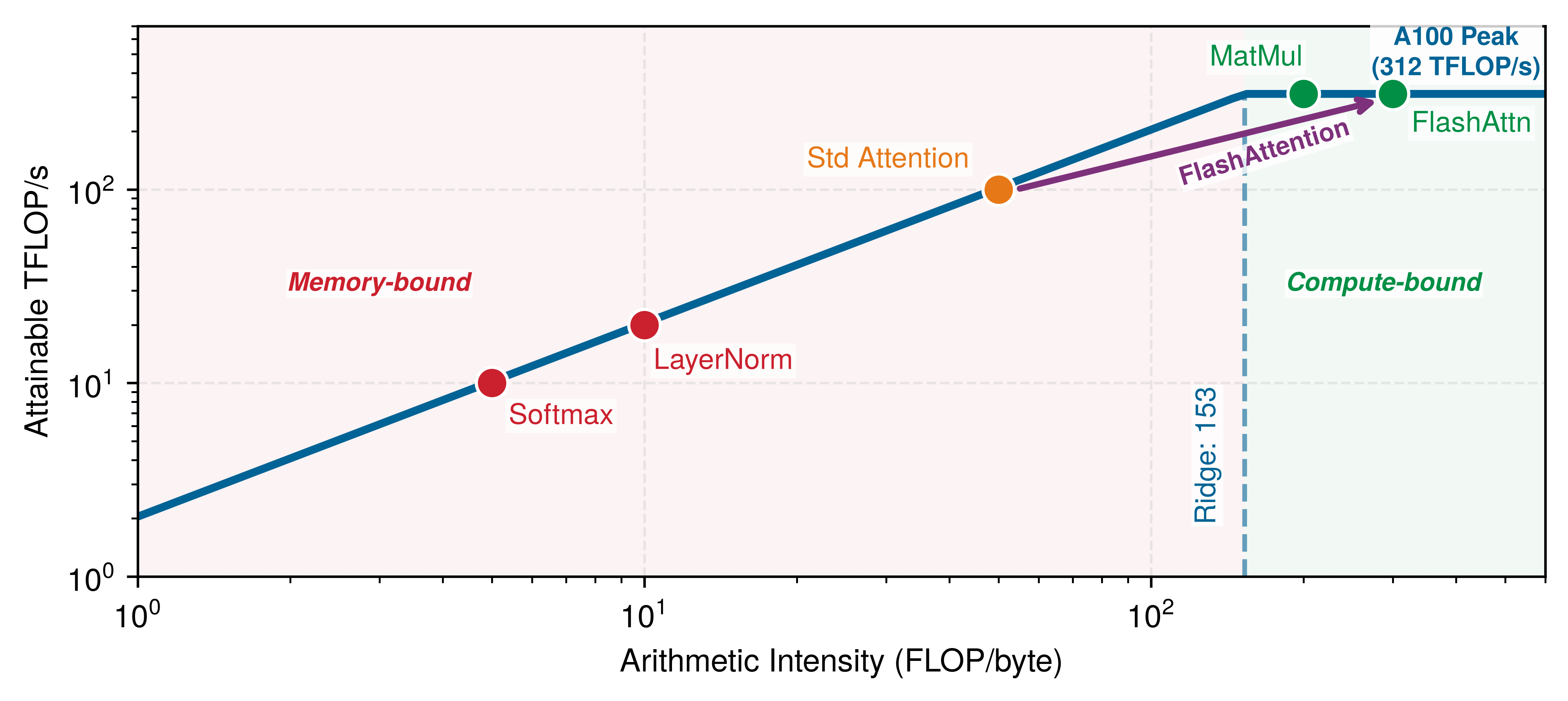
- Diagnose compute-, memory-, and data-bound training bottlenecks with roofline analysis and profiling evidence
- Apply mixed precision, checkpointing, gradient accumulation, and FlashAttention to fit accelerator memory and throughput limits
- Design single-machine training pipelines with prefetching, overlap, batching, and systematic re-profiling
- Evaluate when to scale beyond one machine using memory, duration, communication, energy, and cost constraints
Running a model once and training it from scratch live on opposite sides of the systems cost curve. Frameworks provide the execution substrate: computational graphs schedule operations, automatic differentiation computes gradients, and hardware abstractions target diverse accelerators. Those mechanisms make a single training step possible; training systems make it repeatable at scale. The same forward/backward/update loop may run many thousands or millions of times while retaining activations, feeding accelerators, and staying within practical memory, time, and budget limits.
Training cost stays flat across scale, then explodes past the large-scale knee.
1 Training cost scaling: The roughly 2,000\(\times\) ratio between this chapter’s two cost anchors illustrates how parameter counts, training-token budgets, hardware generations, and accelerator fleets can compound; it is not a controlled comparison of disclosed training bills. OpenAI’s GPT-2 report documents the model and training setup but does not disclose training cost (Radford et al. 2019). Exact GPT-4 training details were also not disclosed, so the GPT-4-class figure is explicitly an industry estimate supported by public reporting and independent infrastructure analysis (Knight 2023; Patel and Wong 2023).
Radford, Alec, Jeffrey Wu, Rewon Child, David Luan, Dario Amodei, and Ilya Sutskever. 2019. Language Models Are Unsupervised Multitask Learners. OpenAI.
Knight, Will. 2023. OpenAI’s CEO Says the Age of Giant AI Models Is Already over. WIRED.
Patel, Dylan, and Gerald Wong. 2023. GPT-4 Architecture, Infrastructure, Training Dataset, Costs, Vision, MoE. SemiAnalysis Blog.
This chapter uses an external order-of-magnitude estimate of approximately $50,000 for GPT-2-scale training and a public estimate near $100M for a GPT-4-class training run.1 Neither figure was disclosed as an audited training bill. This training cost asymmetry reflects the difference between evaluating a trained model for a defined request and repeatedly executing forward, backward, and update computations across a training corpus.
For GPT-2, the chapter uses roughly 3.00 × 10⁹ floating-point operations per token for a forward evaluation, following the parameter-based accounting associated with the architecture in the GPT-2 technical report (Radford et al. 2019). The total budget of 1.50 × 10²¹ FLOPs corresponds to roughly 167 billion token positions when forward and backward work is approximated as three times the forward cost. This accounting estimate is not a claim that GPT-2 executed that many complete inference requests. The scale makes training systems engineering a distinct discipline and shows how access to training infrastructure can constrain participation in AI development.
Definition 1.1: Training systems
Machine learning training systems are software-hardware systems that execute the iterative optimization loop (forward pass, loss computation, backward pass, and parameter update) to minimize a loss function over a training dataset.
- Significance: Training memory cost is 8× the inference memory cost per parameter in a standard mixed-precision Adaptive Moment Estimation (Adam) setup: a 7B-parameter model requires 14 GB (FP16 weights) + 14 GB (FP16 gradients) + 28 GB (FP32 master weights) + 56 GB (Adam first and second moments in FP32) = 112 GB at least, before accounting for activation storage. This multiplier is a major reason a model that runs inference on one GPU requires multiple GPUs for training.
- Distinction: Unlike inference systems, which execute a single forward pass and discard intermediate activations, standard backpropagation stores the tensors needed by the backward pass, creating a footprint that grows with model depth and batch size.
- Common pitfall: A frequent misconception is that training failures are compute problems. A common failure is an out-of-memory (OOM) error, a memory-management problem: tensors saved for backpropagation accumulate during the forward pass and can exhaust memory before the first gradient is computed.
Three characteristics distinguish training workloads from general-purpose computing:
- Computational intensity: The 1.50 × 10²¹ FLOPs budget spread over days of wall-clock time demands sustained PFLOP/s-scale throughput from hardware whose realized large-model throughput is often far below theoretical peak (Narayanan et al. 2021; Chowdhery et al. 2022).
- Memory pressure: Storing 1.5B weights requires 6 GB in FP32; the Adam optimizer adds two state tensors per parameter, consuming another 12 GB. Activation memory adds a workload-dependent footprint governed by architecture, sequence length, batch size, precision, and checkpointing, and the combined state can exceed a single accelerator’s capacity.
- Data dependencies: Each gradient update depends on the result of the previous one, creating sequential bottlenecks that limit how much parallelism the system can exploit.
2 Gradient checkpointing (activation checkpointing): Backpropagation retains the forward values required by each backward rule. Checkpointing saves selected values and recomputes others during backward, trading additional work for lower activation memory. The \(\sqrt{N_L}\) checkpoint placement and its associated recomputation cost describe the classical schedule analyzed by Chen et al. (2016) rather than every checkpointing implementation. Section 1.5.5.2 works through that schedule for GPT-2’s layer count.
Chen, Tianqi, Bing Xu, Chiyuan Zhang, and Carlos Guestrin. 2016. “Training Deep Nets with Sublinear Memory Cost.” arXiv Preprint arXiv:1604.06174.
3 Mixed-precision training: Uses lower precision for selected computation and storage while retaining higher precision where accumulation or numerical range requires it. A common FP16 recipe maintains FP32 master weights and uses loss scaling to reduce gradient underflow (Micikevicius et al. 2017). BF16 (“Brain Floating Point,” from Google Brain (Wang and Kanwar 2019)) matches FP32’s 8-bit exponent range and therefore usually avoids dynamic loss scaling, though the exact state and accumulation precision depend on the optimizer and implementation.
Micikevicius, Paulius, Sharan Narang, Jonah Alben, Gregory Diamos, Erich Elsen, David Garcia, Boris Ginsburg, et al. 2017. “Mixed Precision Training.” arXiv Preprint arXiv:1710.03740.
Wang, Shibo, and Pankaj Kanwar. 2019. BFloat16: The Secret to High Performance on Cloud TPUs.
Each challenge points to a different kind of fix. Computational intensity pushes the system toward higher accelerator utilization and lower-precision arithmetic. Memory pressure calls for techniques such as gradient checkpointing,2 a specific application of rematerialization (discarding and recomputing intermediate values to save memory, from ML Frameworks) that trades recomputation for reduced activation storage, and mixed-precision training,3 which reduces the memory footprint of weights and activations. Data dependencies motivate pipeline designs that overlap computation with data movement, building directly on the data loading throughput optimized in Data Engineering so the accelerator never sits idle waiting for the next batch. The current chapter focuses on single-machine and single-node multi-GPU training; scaling to hundreds of machines across network boundaries introduces communication and fault tolerance challenges beyond this chapter’s scope.
The staged system pipeline: Identifying “accelerator bubbles”
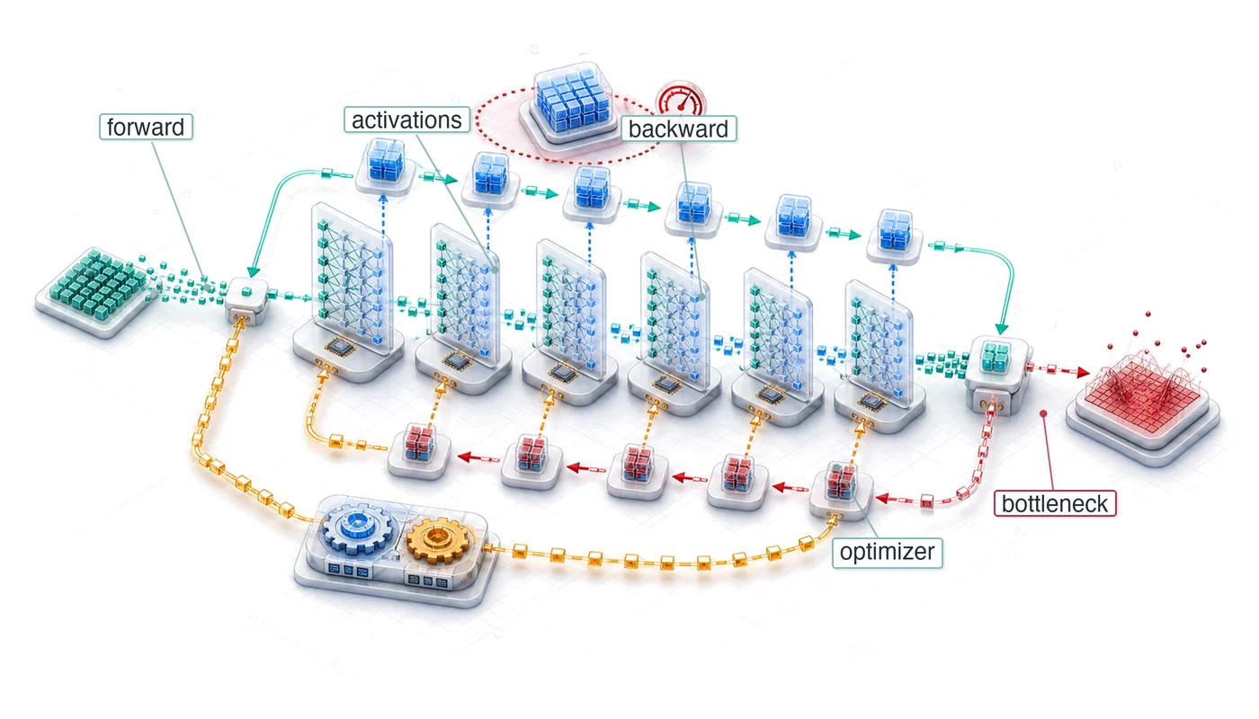
A training system is not a single loop; it is a staged system pipeline. Reaching high accelerator utilization requires analyzing training as a factory floor where four distinct stages coordinate to keep the ALUs busy:
- Data Loading & Preprocessing (CPU/Storage): Fetching raw bits from Non-Volatile Memory Express (NVMe), decoding, and augmenting on CPU cores.
- Host-to-Device Transfer (PCIe): Moving the processed batch over the PCIe bus into GPU memory via direct memory access.
- Forward/Backward Pass (Accelerator): Propagating activations and gradients through layers on the GPU.
- Parameter Synchronization (Interconnect): Exchanging gradients between accelerators over the available fabric. NVLink provides up to 900 GB/s in the H100 configuration used later, while other systems may use PCIe or a network interconnect.
Any mismatch in the throughput of these stages creates accelerator bubbles, intervals in which some accelerator resources are idle or underutilized while waiting for another stage. A systems engineer reduces these bubbles through techniques such as asynchronous prefetching and pipeline overlap, aiming to make the next batch available before the current step needs it. Section 1.4 develops the quantitative tools for measuring and reducing these bubbles.
The chapter follows that dependency chain. The iron law of training performance comes first as a specialized application of the general iron law (Iron Law of ML Systems), separating total operations, peak throughput, and utilization. That equation provides the accounting system for the mathematical foundations that follow: neural-network computation as a workload, optimizer behavior, backpropagation mechanics, and arithmetic intensity. Once the costs are visible, the chapter turns to the training pipeline itself, where data loading, forward pass, backward pass, and parameter updates each constrain the next. The optimization sections then target the terms exposed by the accounting: mixed-precision training, FlashAttention, gradient accumulation, checkpointing, and data prefetching. Scaling beyond one accelerator comes last, after the single-machine levers expose communication overhead as the next bottleneck.
Before formalizing the iron law, consider how these constraints interact in practice. The theoretical framework matters because failures are expensive: a single gradient explosion can erase days of computation worth thousands of dollars.
War Story 1.1: The PaLM loss spikes (2022)
Context: PaLM’s 540-billion-parameter run used 6,144 Tensor Processing Unit (TPU) v4 chips across two 3,072-chip Pods connected through Google’s data-center network and suffered severe training-instability spikes absent from smaller runs (Chowdhery et al. 2022).
Failure mode: The training loss spiked roughly 20 times despite gradient clipping. The spikes occurred at highly irregular intervals, sometimes late in training, never appeared in smaller models, and had no identified principled mitigation.
Impact: Each recovery discarded recent progress on an expensive 6,144-chip run, so reproducible checkpoints and repeatable data order were prerequisites for replay.
Response: Engineers restarted training from an uncorrupted checkpoint roughly 100 steps prior to each spike and skipped approximately 200–500 data batches around the failure window.
Systems lesson: Operational fault tolerance directly governs the utilization factor \(\eta_{\text{hw}}\) in the iron law of training performance (equation 1). Automated loss-spike detection, checkpoint cadence, and batch skipping are core system mechanisms required to protect cluster compute efficiency.
Iron Law of Training Performance
PaLM’s loss spikes illustrate a broader point: instability at frontier scale is not a rare accident but a predictable consequence of pushing computational intensity, memory pressure, and data dependencies simultaneously. Each of those three characteristics is individually manageable, yet their interactions produce failure modes that operational recovery alone cannot prevent. Diagnosing which factor dominates a given failure, and quantifying the cost of each, requires a formal decomposition of training time into its physical constituents.
The iron law provides exactly that organizing framework: it decomposes training time so that every optimization technique maps to a specific term in the equation. This is a specialized application of the general iron law of ML systems introduced in Iron Law of ML Systems, focused specifically on maximizing computational throughput.
Definition 1.2: The iron law of training performance
The iron law of training performance expresses training time through the workload’s operation count and its effective achieved throughput: \[T_{\text{train}} = \frac{O}{R_{\text{peak}} \times \eta_{\text{hw}}} \tag{1}\]
Here \(\eta_{\text{hw}}\) is an effective end-to-end utilization factor, the achieved model-operation rate divided by the relevant hardware peak. Data stalls, communication, synchronization, launch overhead, and inefficient kernels all reduce this factor. Prefetching and overlap can hide part of those costs but do not guarantee their removal.
- Significance: The three factors identify three distinct optimization levers: \(O\) (reducible by algorithmic changes, fewer training tokens, or later model-compression methods such as pruning and distillation), \(R_{\text{peak}}\) (changed by hardware and the selected precision), and \(\eta_{\text{hw}}\) (the effective utilization factor and primary systems target; Narayanan et al. (2021) measured 44 to 52 percent of theoretical peak throughput across GPT models trained on A100 clusters). Model Compression defines the compression techniques; here they serve only to show where such methods enter the accounting.
- Distinction: The general iron law exposes data movement, computation, and latency separately. This training form folds every source of lost throughput into \(\eta_{\text{hw}}\), making it useful for budget accounting but insufficient for diagnosing which underlying term is responsible.
- Common pitfall: A frequent misconception is that \(\eta_{\text{hw}}\) is fixed by hardware. System efficiency is a pipeline property: memory bandwidth saturation, kernel launch overhead, and synchronization barriers each reduce \(\eta_{\text{hw}}\) independently, and diagnosing which factor dominates requires profiling rather than reading hardware specs.
Equation 1 reveals three levers for improvement: reduce total operations through algorithmic innovation, increase peak throughput through hardware utilization, or improve utilization through better pipeline orchestration. Each optimization technique in this chapter pulls one or more of these levers, as summarized in table 1.
| Technique | Term Affected | Mechanism |
|---|---|---|
| Mixed Precision (FP16/BF16) | Peak Throughput ↑ | Uses supported lower-precision hardware paths |
| Data Prefetching | Utilization ↑ | Reduces accelerator idle time waiting for data |
| Gradient Checkpointing | Memory ↓, Operations ↑ | Reduces saved activations by recomputing selected values |
| Gradient Accumulation | Memory ↓, Synchronization ↓ | Builds an effective batch from serialized micro-batches |
| Operator Fusion | Memory Traffic ↓, Overhead ↓ | Avoids intermediate transfers and reduces kernel launches |
| FlashAttention | Memory Traffic ↓, Utilization ↑ | Same asymptotic FLOPs, much lower HBM IO; backward recomputation may add FLOPs |
A caveat: the iron law focuses on execution efficiency—how fast the hardware processes a given workload. It does not capture data-side factors such as data quality, dataset size, or curriculum design, which affect how many total operations \(O\) are needed to reach a target accuracy. A cleaner dataset or a better data mix can reduce the number of epochs required, shrinking \(O\) without touching hardware at all. Holding the workload fixed, the question is how to execute it as fast as possible.
Actual training throughput remains below the arithmetic peak whenever kernels, data delivery, or communication leave resources idle. Scaling to multiple accelerators introduces additional communication overhead, a trade-off quantified in section 1.6.
Checkpoint 1.1: The physics of training
Training speed is governed by the utilization of hardware peaks.
Utilization gap
The iron law provides a static framework for reasoning about training performance, but the history of deep learning reveals how the binding constraint has shifted over time as hardware and algorithms co-evolved. In 1986, Rumelhart and colleagues popularized backpropagation for multilayer neural networks (Rumelhart et al. 1986). In 2012, AlexNet trained an ImageNet classifier in five to six days on two GPUs (Krizhevsky et al. 2012), demonstrating how well neural-network parallelism mapped to graphics hardware. By 2017, transformers (Vaswani et al. 2017) shifted attention toward large-scale sequence modeling and high-throughput accelerator kernels. GPT-3 in 2020 consumed about \(3.14 \times 10^{23}\) FLOPs (Brown et al. 2020), making utilization \((\eta_{\text{hw}})\) critical. By 2023, training efficiency improved through the techniques examined in this chapter: FlashAttention reduces memory traffic while improving \(\eta_{\text{hw}}\); gradient checkpointing trades additional \(O\) for memory capacity; mixed precision increases \(R_{\text{peak}}\). Each innovation addresses a specific iron-law bottleneck.
Vaswani, Ashish, Noam Shazeer, Niki Parmar, Jakob Uszkoreit, Llion Jones, Aidan N. Gomez, Lukasz Kaiser, and Illia Polosukhin. 2017. “Attention Is All You Need.” Advances in Neural Information Processing Systems (NeurIPS) 30: 5998–6008.
Running example: Training GPT-2
In inference, GPT-2 serves as the Bandwidth Hog lighthouse. Here it recurs as the chapter’s stable workload for testing each training cost and optimization.
Lighthouse 1.1: Lighthouse example: Training GPT-2
Context: GPT-2 (1.5 billion parameters) serves as the primary case study because it is large enough to expose meaningful compute, activation, and optimizer-state constraints while remaining easier to analyze than frontier-scale models. Whether it requires distributed training depends on precision, optimizer state, activation memory, hardware capacity, and the target training time. Table 2 maps each model property to the systems constraint it creates:
Table 2: GPT-2 (1.5 Billion Parameters) Lighthouse Model Specifications: Parameter count, architecture depth, dataset size, and total training compute mapped to their systems implications. Each row pairs a model property with the engineering constraint it creates—memory footprint for weights, activation pressure from pipeline depth, I/O throughput requirements, and parallelization demand.
| Property | Specification | Systems Implication |
|---|---|---|
| Parameters | 1.5B (XL) | Requires ~3 GB (FP16) or ~6 GB (FP32) for weights alone. |
| Architecture | 48 Layers, 1600 Dim | Deep pipeline creates heavy activation memory pressure. |
| Dataset | WebText (40 GB) | Preprocessing, shuffling, and delivery must sustain the selected training configuration. |
| Compute | ~ 1.50 × 10²¹ FLOPs | Training duration depends on achieved throughput and accelerator count. |
Mechanism: Training GPT-2 couples a total operation count of \(O \approx 6 \cdot P \cdot D_{\text{tokens}}\), or 1.50 × 10²¹ FLOPs, with a strict memory footprint \(M_{\text{state}} = M_{\text{weights}} + M_{\text{grads}} + M_{\text{opt}} + M_{\text{act}}\). Balancing execution time \(T_{\text{train}} = \frac{O}{R_{\text{peak}} \cdot \eta_{\text{hw}}}\) requires orchestrating data ingestion, activation memory, and compute throughput within accelerator high-bandwidth memory (HBM) capacity.
Not all training workloads are compute bound. Recommendation models like DLRM are dominated by massive embedding tables (100B to 10T parameters, mostly embeddings) that make them memory bandwidth bound rather than compute bound. For such workloads, the first scaling problem is often capacity: splitting the embedding tables across devices so the model fits at all. The remainder of this chapter focuses on dense, compute-intensive training using GPT-2 as the primary worked example.
Training systems occupy a critical position in the machine learning pipeline: they consume prepared data from upstream engineering (Data Engineering) and produce trained model artifacts that later systems must deploy and monitor. Data quality directly impacts training stability, while training efficiency determines iteration velocity during model development. The same pressure appears at three scales. At data scale, petabyte datasets require efficient I/O pipelines and distributed storage. At model scale, billion-parameter models force the system to decide whether to replicate the model across batches with data parallelism4 or split the model across devices with model parallelism.5 At infrastructure scale, coordinating thousands of accelerators introduces communication overhead that can dominate training time. These challenges are why the workflow contracts from ML Workflow matter during training: orchestration decisions shape both scientific iteration and systems cost.
4 Data parallelism: Replicates the full model on every device, splitting only the data. Each device computes gradients independently, then an AllReduce operation synchronizes them—adding communication volume proportional to model size at every step. This synchronization tax limits scaling efficiency: doubling accelerators rarely halves training time once communication becomes the bottleneck.
5 Model parallelism: Partitions the model’s layers across devices when it exceeds single-device memory. Activations must transfer between devices at every partition boundary, and naive partitioning creates “pipeline bubbles” where downstream devices idle while waiting. Microbatch pipelining, as in GPipe and PipeDream, recovers much of this lost efficiency (Huang et al. 2019; Narayanan et al. 2019).
Narayanan, Deepak, Aaron Harlap, Amar Phanishayee, Vivek Seshadri, Nikhil R. Devanur, Gregory R. Ganger, Phillip B. Gibbons, and Matei Zaharia. 2019. “PipeDream: Generalized Pipeline Parallelism for DNN Training.” Proceedings of the 27th ACM Symposium on Operating Systems Principles, 1–15. https://doi.org/10.1145/3341301.3359646.
GPT-2’s 40 GB WebText corpus sits at the lower end of this data scale spectrum. Larger corpora can change the data path qualitatively.
Systems Perspective 1.1: The 10 GB to 10 TB scale factor
In a memory-resident regime, a corpus may fit in system RAM and avoid repeated storage reads after caching, though preprocessing and transfer costs remain. In a streaming regime, the corpus exceeds local memory and the system must orchestrate storage reads, preprocessing, caching, and delivery throughout training. The appropriate design may include multiple workers, prefetching, local caches, or distributed storage, depending on which stage limits throughput.
Scale therefore changes more than the amount of data; it transforms the system’s physics.
These scaling challenges translate into concrete workflow requirements. Training workflows consist of interdependent stages—data preprocessing, forward and backward passes, and parameter updates—extending the neural network concepts from Neural Computation. System constraints often dictate performance limits: accelerators with high compute-to-bandwidth ratios are frequently bottlenecked by memory bandwidth, where data movement between memory hierarchies is slower than the computations themselves (Hennessy and Patterson 2017). In distributed setups, synchronization across devices introduces additional latency, with interconnect performance (NVLink, InfiniBand) critically affecting throughput.6
Hennessy, John L., and David A. Patterson. 2017. Computer Architecture: A Quantitative Approach. 6th ed. Morgan Kaufmann.
6 Transformer training interconnect sensitivity: Self-attention’s \(\mathcal{O}(S^2)\) memory and compute scaling increases activation size with sequence length. In pipeline parallelism, activations cross devices at model-partition boundaries, while data parallelism synchronizes gradients whose volume scales with parameter count. The resulting communication cost depends on the parallelism strategy, topology, message size, and degree of overlap, making interconnect choice a first-order training-system decision.
The same hardware-software boundary that frameworks exposed in ML Frameworks is central here. Mixed-precision training emerged from recognizing that Tensor Core hardware could accelerate reduced-precision arithmetic. Gradient checkpointing arose from memory capacity constraints. Training systems engineering is the work of matching those algorithmic choices to the physical limits of the machine.
These scaling challenges share a common thread: every bottleneck traces back to the cost of specific mathematical operations. Dense matrix multiplication is a well-studied systems kernel (Goto and Geijn 2008), while activation functions consume memory bandwidth and optimizer states increase the resident memory footprint. Designing systems to execute these operations at scale begins with accounting for each cost separately.
Goto, Kazushige, and Robert A. van de Geijn. 2008. “Anatomy of High-Performance Matrix Multiplication.” ACM Transactions on Mathematical Software 34 (3): 1–25. https://doi.org/10.1145/1356052.1356053.
Self-Check: Question
A 1,024-GPU training run has its prefetching pipeline well staged: PCIe is saturated overlapping with compute and gradient AllReduce is hidden behind the next forward pass. Profiling reports 38 percent MFU. Under the simplified iron law of training performance (\(T_{\text{train}} = \frac{O}{R_{\text{peak}} \times \eta_{\text{hw}}}\)), which lever is the most actionable target for the next engineering investment, and why?
- Hardware utilization \(\eta_{\text{hw}}\), because with external data movement and communication already overlapped, the remaining gap to peak throughput consists of kernel-level memory stalls, launch latency, and small tile overheads that profiling can isolate.
- Peak hardware throughput \(R_{\text{peak}}\), because purchasing next-generation accelerators is the only mechanism that directly changes realized MFU.
- Total operations \(O\), because reducing model operations is the only permissible systems modification when communication is hidden.
- Dataset size \(D_{\text{tokens}}\), because shrinking training tokens mathematically raises the hardware utilization factor \(\eta_{\text{hw}}\).
When a team transitions a model from FP32 training to mixed-precision (FP16/BF16) on Tensor Core accelerators without changing the model architecture, batch size, or dataset, which term of the Iron Law of Training Performance (\(T_{\text{train}} = \frac{O}{R_{\text{peak}} \times \eta_{\text{hw}}}\)) is most directly improved?
- Total operations \(O\), because lower numerical precision halves the number of multiplications required in each matrix multiplication.
- Hardware utilization \(\eta_{\text{hw}}\), because mixed precision automatically eliminates all GPU pipeline bubbles and CPU data stalls.
- Peak throughput \(R_{\text{peak}}\), because Tensor Cores provide a substantially higher theoretical FLOP/s ceiling for reduced-precision matrix operations compared to standard FP32 execution units.
- Data volume \(D_{\text{tokens}}\), because lower precision requires fewer training tokens for the loss to converge.
Explain the scope conditions under which the simplified Iron Law of Training Performance (\(T_{\text{train}} = \frac{O}{R_{\text{peak}} \times \eta_{\text{hw}}}\)) accurately models training duration, and identify why it fails for a small-batch debugging session.
All large-scale deep learning models, including recommendation models with multi-terabyte embedding tables (such as DLRM), are primarily compute-bound workloads where training speed is strictly governed by Tensor Core TFLOP/s.
Place the following milestones in the historical evolution of deep learning training systems in chronological order, reflecting how the binding constraint shifted:
- Transformers shift sequence modeling toward high-throughput dense matrix multiplication and large activation footprints.
- Backpropagation is popularized for multilayer neural networks, establishing the algorithmic foundations of gradient descent.
- Large-scale foundation models (such as GPT-3 requiring \(\approx 3.14 \times 10^{23}\) FLOPs) make hardware utilization \(\eta_{\text{hw}}\) and multi-accelerator scaling critical.
- AlexNet demonstrates that neural network training parallelism maps effectively to GPUs, training ImageNet in under a week.
- IO-aware algorithms (such as FlashAttention) and memory-compute trade-offs (gradient checkpointing) co-evolve to overcome memory bandwidth and capacity walls.
Mathematical Foundations
Matrix multiplication is just \(\mathbf{C} = \mathbf{A}\mathbf{B}\) in notation, but training GPT-2 repeatedly executes this operation on matrices too large to remain entirely in the fastest memory. Tensor Cores accelerate eligible matrix operations, while choices such as rectified linear unit (ReLU) versus sigmoid affect the cost, fusion opportunities, and memory behavior of the surrounding elementwise kernels. Neural Computation established what neural network operations compute and why they enable learning; the systems question is what they cost in FLOPs, memory, and bandwidth when those operations execute at scale.
Four dimensions structure this cost analysis:
- FLOP counts of the matrix operations that dominate dense neural-network training.
- Memory requirements for storing activations and optimizer states simultaneously.
- Bandwidth demands that determine whether operations are compute bound or memory bound.
- Arithmetic intensity classifications that guide optimization strategy selection.
Together, these dimensions provide the vocabulary for analyzing the computational intensity, memory pressure, and data dependencies introduced in Training Systems Fundamentals.
Neural network computation
Neural network training consists of repeated matrix operations and nonlinear transformations. These operations are conceptually simple but create the system-level challenges that dominate modern training infrastructure. The introduction of backpropagation7 by Rumelhart et al. (1986) and the development of efficient matrix computation libraries such as Basic Linear Algebra Subprograms (BLAS)8 (Dongarra et al. 1988) laid the groundwork for modern training architectures.
7 Backpropagation provenance: The algorithm was independently derived by Linnainmaa (1970) for automatic differentiation of computer programs and by Werbos (1974) in a Harvard PhD thesis on economic modeling—over a decade before Rumelhart et al. (1986) popularized it for neural networks. This delay between derivation and broad adoption recurs in ML systems history: attention mechanisms predated transformers by decades, but the 2017 Transformer showed that attention-heavy models could train efficiently on contemporary GPU systems; later TPU and GPU clusters enabled much larger deployments. A framework’s backward pass traverses the computational graph in reverse topological order and applies the chain rule; independent subgraphs may expose parallel work during that traversal.
Linnainmaa, Seppo. 1970. “The Representation of the Cumulative Rounding Error of an Algorithm as a Taylor Expansion of the Local Rounding Errors.” Master's thesis, University of Helsinki.
Werbos, Paul. 1974. “Beyond Regression: New Tools for Prediction and Analysis in the Behavioral Sciences.” PhD thesis, Harvard University.
Rumelhart, David E., Geoffrey E. Hinton, and Ronald J. Williams. 1986. “Learning Representations by Back-Propagating Errors.” Nature 323 (6088): 533–36. https://doi.org/10.1038/323533a0.
8 BLAS (basic linear algebra subprograms): The original BLAS specification standardized reusable Fortran-callable vector operations (Lawson et al. 1979); later BLAS extensions added matrix-vector and matrix-matrix routines, giving the familiar Level 1, Level 2, and Level 3 hierarchy (Dongarra et al. 1988). Training is dominated by Level 3 operations precisely because their high arithmetic intensity—\(\mathcal{O}(n)\) FLOP/byte—can sustain high compute utilization. Frameworks commonly dispatch dense matrix multiplication to optimized libraries such as cuBLAS and oneDNN or to compiler-generated kernels.
Lawson, Charles L., Richard J. Hanson, David R. Kincaid, and Fred T. Krogh. 1979. “Basic Linear Algebra Subprograms for Fortran Usage.” ACM Transactions on Mathematical Software 5 (3): 308–23. https://doi.org/10.1145/355841.355847.
Dongarra, Jack J., Jeremy Du Croz, Sven Hammarling, and Richard J. Hanson. 1988. “An Extended Set of FORTRAN Basic Linear Algebra Subprograms.” ACM Transactions on Mathematical Software 14 (1): 1–17. https://doi.org/10.1145/42288.42291.
Mathematical operations in neural networks
Forward propagation, in its simplest case, involves two operations: matrix multiplication and activation function application. Matrix multiplication implements the linear transformation at each layer. At layer \(\ell\), the computation can be described as (following the row-vector convention established in Neural Computation): \[ \mathbf{A}^{(\ell)} = f\left(\mathbf{A}^{(\ell-1)}\mathbf{W}^{(\ell)} + \mathbf{b}^{(\ell)}\right) \] where:
- \(\mathbf{A}^{(\ell-1)}\) represents the activations from the previous layer (or the input layer for the first layer), with each row being a sample in the batch,
- \(\mathbf{W}^{(\ell)} \in \mathbb{R}^{n_{\ell-1} \times n_\ell}\) is the weight matrix at layer \(\ell\), which contains the parameters learned by the network,
- \(\mathbf{b}^{(\ell)}\) is the bias vector for layer \(\ell\),
- \(f(\cdot)\) is the activation function applied elementwise (for example, ReLU, sigmoid) to introduce nonlinearity.
Matrix operations
Matrix multiplication formulation established that forward propagation reduces to chains of matrix multiplications, and Core computational primitives catalogued the computational primitives—general matrix multiplication, convolution, and dynamic attention—that every architecture shares. Training amplifies these patterns: each operation executes not once but billions of times, and each forward pass is paired with a backward pass that roughly doubles the computational cost. Understanding which matrix operations dominate—and how their shapes change between forward and backward passes—reveals why specific system designs and optimizations emerged for training.
Matrix multiplication dominance has driven both algorithmic and hardware innovations. Early neural network implementations relied on standard CPU-based linear algebra libraries, but the scale of modern training demanded specialized optimizations. Strassen’s algorithm9 reduced the naive \(\mathcal{O}(n^3)\) complexity to approximately \(\mathcal{O}(n^{2.807})\) (Strassen 1969), and contemporary hardware-accelerated libraries like cuBLAS (NVIDIA 2024) continue pushing computational efficiency limits.
9 Strassen’s algorithm: Achieves \(\mathcal{O}(n^{2.807})\) by replacing one of eight sub-multiplications with additions, but training systems rarely benefit. The recursion disrupts the regular memory-access patterns that Tensor Cores exploit, and accumulated rounding errors across billions of training iterations can destabilize convergence. In practice, mainstream general matrix multiplication libraries such as cuBLAS leave the dominant training matrix multiplications to highly optimized blocked \(\mathcal{O}(n^3)\) kernels with superior hardware utilization rather than recursive Strassen variants.
Strassen, Volker. 1969. “Gaussian Elimination Is Not Optimal.” Numerische Mathematik 13 (4): 354–56. https://doi.org/10.1007/bf02165411.
NVIDIA. 2024. cuBLAS: CUDA Basic Linear Algebra Subprograms.
This computational dominance has driven system-level optimizations: blocked matrix computations that parallelize across multiple units, and memory hierarchies designed for the access patterns of both forward and backward passes. As neural architectures grew, weight and activation matrices both had to remain accessible for backpropagation, and hardware evolved to serve these dense multiplication patterns within growing memory budgets. To illustrate the scale of these operations concretely, consider the attention layer computations in our GPT-2 lighthouse model.
A single GPT-2 layer makes the scale of these computations concrete.
Napkin Math 1.1: GPT-2 attention layer computation
Each GPT-2 layer performs attention computations that exemplify dense matrix multiplication demands. For one GPT-2 transformer layer (all heads combined) with batch size \(B\) = 32, sequence length \(S\) = 1024, and hidden dimension \(d\) = 1600:
Query, Key, Value Projections (the three linear transformations that create attention inputs—3 separate matrix multiplications): \[\begin{gather*} \text{FLOPs} = 2 \times 3 \times (B \times S \times d \times d) \\ = 2 \times 3 \times (32 \times 1024 \times 1600 \times 1600) \approx 503 \text{ billion FLOPs} \end{gather*}\] Attention matmuls (\(\mathbf{Q}\mathbf{K}^\top\) and \(\mathbf{A}_{\text{attn}}\mathbf{V}\)): \[\begin{gather*} \text{FLOPs}_{QK} = 2 \times B \times N_{\text{heads}} \times S \times S \times d_{\text{head}} = 107.4 \text{ billion FLOPs} \\ \text{FLOPs}_{\text{Attn}\times V} = \text{FLOPs}_{QK};\quad \text{pair total} \approx 214.8 \text{ billion FLOPs} \end{gather*}\] Output projection (attention output \(\rightarrow\) hidden): \[ \text{FLOPs} = 2 \times B \times S \times d \times d \approx 168 \text{ billion FLOPs} \] Feed-Forward Network (Two linear transformations with expansion factor 4): \[ \text{FLOPs} \approx 16 \times B \times S \times d^2 \] Computation Scale
- Per-layer forward total (QKV 503 + attention 214.8 + output proj 168 + FFN): ~2228.01 GFLOP
- With 48 layers in GPT-2: ~320.8 TFLOP per training step
- Across this illustrative 50,000 steps scenario: ~16041.7 PFLOP
Systems insight: A V100 GPU (125 TFLOP/s peak with Tensor Cores, 15.7 TFLOP/s without) would require 2.6 s for the modeled attention-plus-FFN training-step estimate at 100 percent utilization (theoretical peak; practical throughput would be lower). Reaching a 180 to 220 ms training step is therefore already a multi-accelerator lower-bound problem: ideal arithmetic alone requires roughly 12 to 15 V100s, and practical systems need additional headroom for utilization losses, communication, and pipeline overhead.
These FLOP counts are not academic bookkeeping. They are the compute term of the iron law made concrete, and they explain why training cost scales as a predictable function of model architecture and sequence length rather than as an unpredictable emergent property.
Matrix-vector and batched operations
Not all operations in neural networks involve large matrix-matrix multiplications. Normalization layers, bias additions, and certain recurrent computations involve matrix-vector operations instead. Although computationally simpler than matrix-matrix multiplication, these operations present distinct system challenges: they exhibit lower hardware utilization due to their limited parallelization potential. A single vector provides insufficient work to keep thousands of accelerator cores busy simultaneously. This characteristic influences both hardware design and model architecture decisions, particularly in networks processing sequential inputs or computing layer statistics.
Recognizing the limitations of matrix-vector operations, the introduction of batching transformed matrix computation in neural networks. By processing multiple inputs simultaneously, training systems convert matrix-vector operations into more efficient matrix-matrix operations. This approach improves hardware utilization but increases memory demands for storing intermediate results. Modern implementations must balance batch sizes against available memory, leading to specific optimizations in memory management and computation scheduling.
The progression from matrix-vector to batched matrix-matrix operations helps explain the hardware design choices in modern accelerators. Google’s first TPU, designed for inference, incorporated a specialized matrix unit and memory hierarchy for dense operations (Jouppi et al. 2017). At a different scale, GPT-3 training used distributed accelerators to execute the matrix-matrix multiplication patterns exposed by large batches (Brown et al. 2020).
Brown, Tom B., Benjamin Mann, Nick Ryder, Melanie Subbiah, Jared Kaplan, Prafulla Dhariwal, Arvind Neelakantan, et al. 2020. “Language Models Are Few-Shot Learners.” Advances in Neural Information Processing Systems 33: 1877–901. https://doi.org/10.48550/arxiv.2005.14165.
Systems Perspective 1.2: Why GPUs dominate training
The matrix operations described in section 1.2.1.2 directly explain data-center training hardware architecture. GPUs became central to large-scale training for three reasons:
- Matrix multiplication’s independent element calculations map well to thousands of GPU cores (NVIDIA A100 has 6,912 CUDA cores).
- Specialized hardware units like Tensor Cores provide substantially higher peak throughput for supported lower-precision matrix operations.
- Blocked matrix computation patterns enable efficient use of GPU memory hierarchy (L1/L2 cache, shared memory, global memory).
When a later illustrative GPT-2 scenario assumes a 2.4\(\times\) V100 mixed-precision speedup, Tensor Core acceleration of eligible matrix multiplications is one source of the gain. The realized end-to-end ratio also depends on nonmatrix operations, memory traffic, and input and communication overhead.
Matrix multiplications dominate training compute, but neural networks require more than linear transformations. Between each layer’s matrix operations, activation functions introduce the nonlinearity that enables networks to learn complex patterns. These functions appear computationally trivial compared to matrix multiplication, yet their implementation characteristics affect training efficiency in ways that matter at scale.
Activation functions
Activation functions like sigmoid, tanh, ReLU, and softmax introduce nonlinearity, but their implementation characteristics also shape training system performance. From a systems perspective, the choice of activation function determines computational cost, hardware utilization, and memory access patterns during backpropagation.
The critical question for ML systems engineers is not what these functions do mathematically, but how their cost behaves at scale. The benchmarks and trade-offs that follow build toward one systems thesis. Because elementwise activations move many more bytes than they compute, their kernels are often bounded by memory bandwidth rather than arithmetic, so the per-operation differences below matter less than their magnitudes first suggest.
Activation costs can accumulate across many elements and layers, but their contribution to end-to-end time depends on tensor shape, fusion, implementation, precision, and hardware. Figure 1 preserves one illustrative Apple M2 timing snapshot from the chapter’s development history. Its benchmark configuration was not recorded, so the values should not be interpreted as reproducible evidence or transferred to other systems. On accelerators, activation kernels are often limited by memory traffic, fusion boundaries, and special-function throughput rather than by scalar CPU instruction latency. The same activation may run as a standalone kernel, fuse with a neighboring operator, or use a compiler-selected approximation. The plotted scalar timing therefore cannot predict its cost inside a compiled training step.
\scalebox{0.9}{%
\begin{tikzpicture}[font=\small\sffamily]
% Standard color definitions
\definecolor{BlueLine}{HTML}{006395}
\definecolor{GreenLine}{HTML}{008F45}
\definecolor{RedLine}{HTML}{CB202D}
\definecolor{OrangeLine}{HTML}{CC5500}

\begin{axis}[
    ylabel={Execution Time (seconds)},
    ymin=0.40,
    width=100mm,
    height=57mm,
    axis lines=left,
    axis line style={thick,-latex},
    ytick={0.4,0.5,...,1.1},
    yticklabel style={font=\footnotesize\sffamily,
    /pgf/number format/.cd, fixed, fixed zerofill, precision=2},
    xticklabel style={font=\footnotesize\sffamily},
    ylabel style={font=\footnotesize\sffamily},
    ymax=1.15,
    enlarge x limits=0.2,
    tick style={draw=black,thin},
    tick align=outside,
    major tick length=1mm,
    xtick={1,2,3,4},
    xticklabels={Sigmoid,Tanh,ReLU,Softmax},
    every axis plot/.append style={
          ybar,
          bar width=0.55,
          bar shift=0pt,
          fill
        }]
      \addplot[RedLine] coordinates {(1,1.1)};
      \addplot[BlueLine] coordinates {(2,0.61)};
      \addplot[GreenLine] coordinates {(3,0.45)};
      \addplot[OrangeLine] coordinates {(4,0.91)};
\end{axis}
\end{tikzpicture}}Modern accelerators can implement these functions through native instructions, polynomial approximations, lookup methods, or fused kernels. ReLU requires a simple threshold operation, while sigmoid, tanh, and exact Gaussian Error Linear Unit (GELU) formulations require more arithmetic or special-function support. The realized latency difference still depends on whether arithmetic, memory traffic, or launch overhead is binding. ReLU may produce zeros that a later system can exploit, but the sparsity fraction depends on the activation distribution and trained model. Softmax10 adds a reduction and normalization across the selected axis. Those dependencies require coordination, though optimized implementations remain highly parallel.
10 Softmax: Computing a numerically stable softmax requires a maximum reduction, exponentiation, a sum reduction, and normalization across the selected axis. Parallel kernels implement these stages with coordinated reductions. FlashAttention restructures the larger attention computation so softmax statistics can be maintained while tiles remain near the compute units.
Table 3 summarizes how these behaviors translate into system constraints.
| Function | Key Advantages | Key Disadvantages | System Implications |
|---|---|---|---|
| Sigmoid | Smooth; bounded output in \((0, 1)\). | Gradients saturate at large magnitudes; output is not zero-centered. | Uses exponential or approximation kernels whose cost depends on the target. |
| Tanh | Smooth; zero-centered output in \((-1, 1)\). | Gradients saturate at large magnitudes. | Uses special-function or approximation kernels similar in structure to sigmoid. |
| ReLU | Simple threshold operation; nonsaturating for positive inputs. | Can produce persistently inactive units. | Often inexpensive and fusible; exploitable sparsity depends on downstream support. |
| Softmax | Produces a normalized distribution over an axis. | Requires reductions and cross-element coordination. | Parallel implementations coordinate maximum, sum, and normalization stages. |
ReLU remains common because it is simple and efficient, while softmax is essential when a model must normalize scores into probabilities. GPT-2 illustrates a different choice through GELU, the Gaussian Error Linear Unit.
Systems Perspective 1.3: The GELU activation choice
Beyond the foundational activation functions covered in Neural Computation (Sigmoid, Tanh, ReLU), modern architectures increasingly adopt smoother alternatives. GPT-2 uses a GELU activation (Radford et al. 2019), the Gaussian Error Linear Unit introduced by Hendrycks and Gimpel (2016) and often implemented with the common tanh-based approximation from that formulation. Its exact definition is: \[
\text{GELU}(x) = x \cdot \Phi(x) = x \cdot \frac{1}{2}\left[1 + \text{erf}\left(\frac{x}{\sqrt{2}}\right)\right]
\] where \(\Phi(x)\) is the cumulative distribution function of the standard normal distribution.
GELU applies a smooth, input-dependent scaling rather than ReLU’s hard threshold. It is deterministic despite its formulation in terms of a Gaussian cumulative distribution. Whether it improves model quality relative to another activation is an empirical property of the architecture and training recipe, not a universal guarantee.
Exact GELU uses erf, while common implementations use a tanh-based approximation such as listing 1. The approximation changes arithmetic cost and introduces a small numerical difference from the exact function. End-to-end impact depends on fusion, tensor size, precision, kernel implementation, and the fraction of runtime spent in activation kernels, so no fixed GELU-to-ReLU ratio applies across systems.
Hendrycks, Dan, and Kevin Gimpel. 2016. “Gaussian Error Linear Units (GELUs).” arXiv Preprint arXiv:1606.08415.
# Fast GELU approximation used in production systems
# Avoids expensive erf() computation while
# preserving activation properties
gelu_approx = (
    0.5 * x * (1 + tanh(sqrt(2 / pi) * (x + 0.044715 * x**3)))
)
The GELU approximation highlights a broader pattern: compute cost is not always the dominant concern. For activation functions, the real bottleneck is often memory bandwidth rather than arithmetic operations. This distinction between compute-bound and memory-bound operations directly affects optimization priorities and recurs throughout the analysis of training bottlenecks.
Dense matrix multiplication can reuse operands across many multiply-accumulate operations, while an unfused elementwise activation typically performs little work for each value read and written. This arithmetic-intensity gap often makes standalone activation kernels memory-sensitive. Fusion can remove intermediate memory traffic, and special-function throughput can still matter for kernels whose arithmetic is not fully hidden. Replacing one activation with another therefore has no fixed wall-clock effect.
Systems Perspective 1.4: Memory bandwidth bottlenecks
Activation functions reveal a critical systems principle: not all operations are compute bound. While matrix multiplications saturate accelerator compute units, activation functions often become memory bandwidth bound for three reasons:
- Elementwise operations perform few calculations per memory access; ReLU performs one operation per load.
- Simple operations complete faster than memory transfer time, limiting parallelism benefits.
- Accelerator compute capability has grown faster than external-memory bandwidth, increasing pressure to reuse data near the compute units.
This is why scalar operation counts alone do not predict activation-kernel latency. The forward pass must account for fusion and activation storage as well as function-evaluation cost when determining whether memory bandwidth limits throughput.
Forward pass operations and their computational characteristics establish the workload that training systems must compute: matrix multiplications dominating FLOPs, activation functions constrained by memory bandwidth. A neural network that only computes predictions, however, learns nothing. Training requires updating model parameters so future predictions improve. The forward pass produces a loss value quantifying how wrong the current predictions are; the question now shifts from how much computation costs to how to use the result to improve.
Optimization algorithms
Optimization algorithms determine, given a loss value and the gradient information it produces, how each parameter should change to reduce future errors. These algorithms govern the learning trajectory, translating gradients into parameter updates that steer the model toward better performance, and their selection has direct system-level implications for computation efficiency, memory requirements, and scalability. The focus here is on the algorithms themselves during training: how they use gradients, how much state they retain, and how their update rules interact with the hardware budget.
Gradient-based optimization methods
Parameter update algorithms introduces gradient descent as the fundamental optimization algorithm: iteratively adjusting parameters in the direction of steepest descent. That conceptual foundation assumed modest networks on single devices. At hardware scale, gradient descent and its variants interact with real physical constraints. The same mathematical operation that elegantly adjusts weights becomes a significant systems challenge when models contain billions of parameters and training data spans terabytes.
Gradient descent
Gradient descent is the mathematical foundation of neural network training, iteratively adjusting parameters to minimize a loss function. In training systems, this mathematical operation translates into specific computational patterns. For each iteration, the system must execute four dependent operations:
- Compute forward pass activations
- Calculate loss value
- Compute gradients through backpropagation
- Update parameters using the gradient values
The computational demands of gradient descent scale with both model size and dataset size. Computing gradients requires storing intermediate activations during the forward pass for backpropagation. These activations consume memory proportional to the depth of the network and the number of examples being processed.
Traditional gradient descent processes the entire dataset before each parameter update. For a training set with one million examples, the system must compute an aggregate gradient over all examples before taking one step. Let \(D\) denote the number of examples in the training dataset, let \(B_{\text{micro}}\) denote the examples resident for one forward/backward pass, and let \(T_{\text{forward+backward per example}}\) denote the amortized forward/backward time per example under the chosen micro-batch execution regime. Gradient accumulation composes multiple micro-batches into one larger effective batch. The peak-memory relation in equation 2 and the step-time relation in equation 3 capture the implementation distinction: \[ \text{Peak Activation Memory} \propto B_{\text{micro}} \times \text{Activation Memory per Example} \tag{2}\] \[ T_{\text{step}} \propto D \times T_{\text{forward+backward per example}} \tag{3}\]
The true cost of training memory formalizes this breakdown by deriving the full training memory equation, including optimizer-state overhead. Full-batch training does not require storing every example’s activations simultaneously if the dataset is streamed or microbatched; peak memory is governed by the examples held in memory at once. The systems problem is still severe: processing \(D=1{,}000{,}000\) examples before each update creates million-example iteration times, reducing the rate at which the model can learn from the data.
Hardware-friendly variants relax the need for an exact full-dataset gradient on every update. Stochastic gradient descent (SGD)11 estimates gradients from sampled examples or mini-batches rather than the entire dataset. This changes update frequency and gradient variance while allowing each update to operate on a bounded working set.
11 Stochastic gradient descent: “Stochastic” from Greek stochastikos (“able to guess”); rather than waiting for an exact full-dataset gradient, SGD updates from sampled examples or mini-batches. Full-batch and stochastic methods can both stream data through bounded micro-batches, so their peak activation memory is determined by the resident micro-batch rather than by dataset size alone. Their central difference is how many sampled gradients contribute to each parameter update.
However, processing single examples creates new system challenges. Modern accelerators achieve peak performance through parallel computation, processing multiple data elements simultaneously. Single-example updates leave most computing resources idle, resulting in poor hardware utilization. The frequent parameter updates also increase memory bandwidth requirements, as weights must be read and written for each example rather than amortizing these operations across multiple examples.
Mini-batch processing
Mini-batch gradient descent emerges as a practical compromise between full-batch and stochastic methods, an algorithm-machine co-design that computes gradients over small batches of examples aligned with modern accelerator architectures (Dean et al. 2012). The batch size \(B\) becomes a key system parameter, influencing both computational efficiency and memory requirements.
Dean, Jeffrey, Greg Corrado, Rajat Monga, Kai Chen, Matthieu Devin, Quoc V. Le, Mark Z. Mao, et al. 2012. “Large Scale Distributed Deep Networks.” In Advances in Neural Information Processing Systems (NeurIPS), edited by Peter L. Bartlett, Fernando C. N. Pereira, Christopher J. C. Burges, Léon Bottou, and Kilian Q. Weinberger, vol. 25, 25. Curran Associates.
Definition 1.3: Batch processing
Batch processing aggregates multiple training examples into tensor operations that amortize fixed per-step overhead across \(B\) examples and can expose more parallel work. Increasing \(B\) may improve occupancy and arithmetic intensity, but it does not guarantee that every operation becomes compute bound.
- Significance: Throughput often increases with batch size until the target hardware is sufficiently occupied, while the number and quality of updates needed for convergence follow a separate workload-dependent curve. Goyal et al. demonstrated a ResNet-50 ImageNet recipe at \(B=8{,}192\) using linear learning-rate scaling and warmup (Goyal et al. 2017). That result is a configuration-specific demonstration rather than a universal critical batch size.
- Distinction: A mini-batch update averages gradients over \(B\) examples. Under independent, similarly distributed samples, the standard deviation of this mean decreases approximately as \(1/\sqrt{B}\). The update processes more data than a single-example update, so its net data movement and time depend on reuse, implementation, and how batch size changes the number of updates required.
- Common pitfall: A frequent misconception is that linear learning-rate scaling (multiplying \(\eta\) by \(B/B_0\)) works at any batch size. It is a training recipe that commonly requires warmup and empirical validation, and its useful range depends on the model, data, optimizer, and target accuracy.
The relationship between batch size and system performance reveals hardware-software trade-offs. The decomposition in equation 4 separates fixed parameter and gradient storage from a batch-dependent activation term: \[ \text{Memory Required} = \text{Parameter Memory} + \text{Gradient Memory} + B \times \text{Activation Memory} \tag{4}\]
Because the activation term scales with \(B\) while parameter and gradient memory stay fixed, doubling the batch doubles the activation working set, and a model that fits comfortably at a small batch can exhaust the 40–80 GB of HBM on a high-end training accelerator once the batch grows. Section 1.3.3.2 works this budget through layer by layer for
Larger batches can enable more efficient computation through improved parallelism and better memory access patterns. Accelerator utilization efficiency demonstrates this trade-off: larger batches generally expose more parallel work to the accelerator, while very small batches can leave compute units underfilled. Linear scaling rules for large-batch training (scale learning rate proportionally to batch size increase) can help maintain convergence speed within an empirically validated range (Goyal et al. 2017).
This establishes a central theme in training systems: the hardware-software trade-off between memory constraints and computational efficiency. Training systems must select batch sizes that maximize hardware utilization while fitting within available memory. The optimal choice often requires gradient accumulation when memory constraints prevent using efficiently large batches, trading micro-batch serialization and some overhead for the same effective batch size.
Adaptive and momentum-based optimizers
Basic SGD applies one learning rate to every parameter, which can make optimization difficult when gradient scales differ substantially across dimensions. Momentum smooths updates using gradient history, RMSprop adapts step sizes per parameter, and Adam combines first-moment tracking with adaptive scaling (Kingma and Ba 2015). These methods consume gradients computed by backpropagation; they do not determine whether those gradients are correct. Their convergence behavior depends on the model and training recipe, while their additional state creates concrete memory and computation costs.
Kingma, Diederik P., and Jimmy Ba. 2015. “Adam: A Method for Stochastic Optimization.” 3rd International Conference on Learning Representations (ICLR).
Momentum-based methods
Momentum methods12 address SGD’s oscillation problem by accumulating a velocity vector across iterations, smoothing out noisy gradient directions. From a systems perspective, this smoothing comes at a cost: the training system must maintain a velocity vector with the same dimensionality as the parameter vector. Parameters plus this auxiliary state therefore occupy twice the parameter storage before gradients and activations are counted.
12 Momentum: Borrowed from physics, where momentum (mass \(\times\) velocity) describes an object’s tendency to continue moving. The metaphor explains the design because accumulated velocity smooths noisy gradients and can reduce the iterations needed for convergence. The systems cost is one additional velocity value per parameter, while Adam maintains two moment values per parameter.
Adaptive learning rate methods
While momentum smooths gradient direction, it does not address the different scales of gradients across parameters. RMSprop13 solves this by maintaining a moving average of squared gradients for each parameter, automatically reducing step sizes for parameters with historically large gradients. This per-parameter adaptation requires storing the moving average \(s_t\), creating memory overhead similar to momentum methods. The elementwise operations in RMSprop also introduce additional computational steps compared to basic gradient descent.
13 RMSprop: Proposed by Geoffrey Hinton in Lecture 6e of his 2012 Coursera course—never published in a peer-reviewed paper, making it perhaps the most influential optimizer disseminated via a slide deck. RMSprop divides the learning rate by a running average of recent gradient magnitudes, adapting step sizes per parameter. This per-parameter adaptation is what Adam inherits as its second moment \(v_t\), directly contributing to Adam’s 3\(\times\) memory overhead described in section 1.2.2.3.
Adam optimization
Adam14 combines the benefits of both momentum and RMSprop: momentum’s gradient smoothing addresses noisy updates, while RMSprop’s adaptive scaling handles parameter-specific step sizes. This combination maintains two moving averages for each parameter. Here \(m_t\) and \(v_t\) are the first- and second-moment buffers, \(\beta_1\) and \(\beta_2\) are their decay factors, and \(\epsilon\) is the numerical-stability constant in the denominator: \[\begin{gather*} m_t = \beta_1 m_{t-1} + (1-\beta_1)\nabla \mathcal{L}(\theta_t) \\[0.5ex] v_t = \beta_2 v_{t-1} + (1-\beta_2)\big(\nabla \mathcal{L}(\theta_t)\big)^2 \\[0.5ex] \hat{m}_t = \frac{m_t}{1-\beta_1^t}, \qquad \hat{v}_t = \frac{v_t}{1-\beta_2^t} \\[0.5ex] \theta_{t+1} = \theta_t - \eta \frac{\hat{m}_t}{\sqrt{\hat{v}_t} + \epsilon} \end{gather*}\]
14 Adam (adaptive moment estimation): The two moving averages are the first moment (momentum) and second moment (uncentered variance) of the gradients, stored for every model parameter. For a 7B model, Adam’s FP32 moment tensors alone consume 56 GB; the full standard mixed-precision training state before activations is 112 GB once FP16 weights, FP16 gradients, FP32 master weights, and Adam moments are counted together.
The system implications of Adam are more substantial than previous methods. The optimizer must store two additional vectors (\(m_t\) and \(v_t\)) for each parameter, tripling the parameter-plus-optimizer-state footprint; for a 100M-parameter model, those auxiliary vectors alone add 800 MB beyond weight storage.
Optimization algorithm system implications
The choice of optimization algorithm creates specific patterns of computation and memory access that influence training efficiency. Optimizer auxiliary memory increases progressively from SGD (no auxiliary state) through Momentum (one velocity vector) to Adam (two moment vectors), as quantified in table 4. These memory costs must be balanced against convergence15 benefits. Adam may require fewer iterations for some workloads, but its per-iteration memory and computation overhead can reduce training speed on memory-constrained systems. At GPT-2 scale, this overhead becomes a first-order memory constraint.
15 Convergence: A run reaches its stopping criterion when the selected training or validation metric no longer improves enough to justify additional work. The required steps depend on the model, data, optimizer, schedule, batch size, and target quality. Fewer steps can reduce wall-clock time and cost, but adaptive optimizers add state whose memory and traffic must be included in the system budget.
| Property | SGD | Momentum | RMSprop | Adam |
|---|---|---|---|---|
| Memory Overhead | None | Velocity terms | Squared gradients | Both velocity and squared gradients |
| Parameter + optimizer state | 1\(\times\) | 2\(\times\) | 2\(\times\) | 3\(\times\) |
| Dense State Access | Parameters and gradients | Adds velocity | Adds squared-gradient state | Adds first- and second-moment state |
| Update Work | Lowest auxiliary work | Adds momentum update | Adds adaptive scaling | Adds moment updates and bias correction |
| Hardware Efficiency | Varies | Varies | Varies | Varies |
| Convergence Behavior | Varies | Varies | Varies | Varies |
The costs quantified in table 4 create a design tension. Adam’s two moment buffers may improve optimization for a given workload, but their memory can reduce the model size or batch size that fits on an accelerator. AdamW16 (Loshchilov and Hutter 2019) decouples weight decay from Adam’s adaptive gradient update without adding another per-parameter state tensor.
16 AdamW (Adam with decoupled weight decay): Standard \(L_2\) regularization enters the gradient and is therefore rescaled by Adam’s adaptive update. AdamW applies weight decay as a separate parameter update, restoring the intended distinction between adaptive gradient scaling and decay (Loshchilov and Hutter 2019). It uses the same moment-buffer structure as Adam, though its effect on model quality remains workload dependent.
Loshchilov, Ilya, and Frank Hutter. 2019. “Decoupled Weight Decay Regularization.” Proceedings of the International Conference on Learning Representations (ICLR).
Napkin Math 1.2: GPT-2 optimizer memory requirements
A representative GPT-2 XL training configuration uses the Adam optimizer with five hyperparameters:
- β₁ = 0.9 (momentum decay)
- β₂ = 0.999 (second moment decay)
- Learning rate: Warmed up from 0 to 2.5e-4 over first 500 steps, then cosine decay
- Weight decay: 0.01
- Gradient clipping: Global norm clipping at 1.0
Math:
For GPT-2’s 1.5B parameters in FP32 (4 bytes each), the memory breaks down across four components:
- Parameters: 1.5B \(\times\) 4 bytes = 6 GB
- Gradients: 1.5B \(\times\) 4 bytes = 6 GB
- Adam State (m, v): 1.5B \(\times\) 8 bytes = 12 GB
- Total static memory: 24 GB
This explains why GPT-2’s 24 GB static training state alone approaches the 32 GB capacity of a V100 before activation storage is counted.
System Decisions Driven by Optimizer
- Mixed precision training (FP16) reduces operation precision but requires keeping FP32 master weights, maintaining the static memory footprint at ~24 GB.
- Gradient accumulation (splitting effective batches into smaller micro-batches) allows effective batch size \(B=512\) despite memory limits.
Systems insight: This illustrative configuration shows how Adam’s moment buffers constrain capacity. Any convergence benefit relative to SGD or momentum must be measured under a matched model, data, schedule, batch size, and stopping criterion.
Framework optimizer interface and scheduling
After optimizer memory is quantified, the framework interface matters because it fixes when that state is read, written, cleared, and preserved across steps. A training loop separates gradient computation from parameter updates so that the system can accumulate gradients, synchronize them, or defer updates without changing the optimizer equations. Listing 2 demonstrates where Adam optimization enters that cycle.
import torch
import torch.nn as nn
import torch.optim as optim

# Initialize Adam optimizer with model parameters and learning rate
optimizer = optim.Adam(
    model.parameters(), lr=0.001, betas=(0.9, 0.999)
)
loss_function = nn.CrossEntropyLoss()

# Standard training loop implementing the four-step optimization cycle
for epoch in range(num_epochs):
    for batch_idx, (data, targets) in enumerate(dataloader):
        # Step 1: Clear accumulated gradients from previous iteration
        optimizer.zero_grad()

        # Step 2: Forward pass - compute model predictions
        predictions = model(data)
        loss = loss_function(predictions, targets)

        # Step 3: Backward pass - compute gradients via autodiff
        loss.backward()

        # Step 4: Parameter update - apply Adam optimization equations
        optimizer.step()
The optimizer.zero_grad() call marks the boundary between one update and the next. Gradients accumulate across calls to backward(), so clearing them explicitly prevents stale gradients from contaminating the next batch. The same accumulation behavior later becomes useful for large effective batch sizes, but only when the training loop manages the boundary deliberately.
The optimizer.step() method is the other boundary: it consumes the current gradients and mutates persistent optimizer state. For Adam optimization, this call implements momentum estimation, squared gradient tracking, bias correction, and the parameter update. Algorithm 1 makes the hidden state explicit so the memory cost remains visible rather than disappearing behind an API call.

In this simplified static-state view, Adam’s two moment buffers occupy twice the parameter storage.
\begin{algorithm} \caption{Adam parameter update (one optimizer step)} \begin{algorithmic} \Require gradient $g_t = \nabla\mathcal{L}(\theta_t)$; step $t$; rate $\eta$; decays $\beta_1,\beta_2$; constant $\epsilon$ \Ensure updated parameter $\theta_{t+1}$; moment buffers $m_t, v_t$ carried to the next step \State $m_t \gets \beta_1 m_{t-1} + (1-\beta_1)\, g_t$ \Comment{first moment (momentum)} \State $v_t \gets \beta_2 v_{t-1} + (1-\beta_2)\, g_t^2$ \Comment{uncentered second moment} \State $\hat{m}_t \gets m_t / (1-\beta_1^{t})$; $\hat{v}_t \gets v_t / (1-\beta_2^{t})$ \Comment{bias correction} \State $\theta_{t+1} \gets \theta_t - \eta\, \hat{m}_t / (\sqrt{\hat{v}_t} + \epsilon)$ \Comment{parameter update} \end{algorithmic} \end{algorithm}
Steps 1 and 2 keep two persistent moment buffers per parameter, so parameters plus optimizer state reach roughly 3\(\times\) the parameter memory before gradients, activations, and FP32 master weights are counted. Framework implementations manage the allocator and access patterns for these optimizer states, but they do not remove the cost. Each Adam step reads the gradient, parameter, first moment, and second moment, then writes back the updated moments and parameter. The abstraction reduces implementation burden; the systems budget still pays for two extra tensors that must occupy memory and move through the hierarchy every step.
Learning rate scheduling integration
The framework’s learning rate scheduling hook changes the optimizer’s trajectory without adding per-parameter state. It adjusts the learning rate \(\eta\) during training, letting the system shape convergence behavior while leaving the underlying optimizer equations intact.
Schedules such as cosine annealing, exponential decay, or step-wise reductions implement that trajectory by changing the step size over time. A scheduler may track the current step, epoch, warmup phase, or other state that must be restored with a checkpoint. It changes \(\eta\) without changing the optimizer’s base update equations; ML Frameworks covers the scheduler interface that wires this in. This separation lets the systems engineer combine base optimization algorithms (SGD, Adam) with scheduling strategies (cosine annealing, linear warmup) without reimplementing the update rule.
The optimization algorithms in the preceding section specify how to update parameters given gradients, but they take those gradients as given. SGD, momentum, and Adam all assume gradient vectors arrive ready-made. In practice, computing gradients for a network with billions of parameters is itself a major computational and memory challenge. The cost of gradient computation, not the cost of the optimizer step, is what makes training so much more expensive than inference.
Backpropagation mechanics
Backpropagation solves the gradient computation problem by tracing error signals backward through the network, systematically attributing responsibility to each parameter for the final prediction error. Its memory and computational requirements reveal why training systems face such substantial resource constraints.
The backpropagation algorithm computes gradients by systematically moving backward through a neural network’s computational graph. Gradient computation and backpropagation establishes the mathematical foundation: the chain rule breaks gradient computation into layer-by-layer operations, with each layer receiving adjustment signals proportional to its contribution to the final error. If terms like “computational graph” or “gradient flow” feel unfamiliar, the factory assembly line analogy in that section is worth revisiting.
At system scale, the question shifts from what backpropagation computes to what it costs. The layer computations from section 1.2.1.1 produce activations that must be retained for the backward pass. Computing \(\frac{\partial \mathcal{L}}{\partial \mathbf{W}^{(\ell)}}\) requires access to these stored activations, creating the training memory equation that gradient checkpointing later exploits.
A simple three-layer network processing MNIST requires kilobytes of activation storage. GPT-2 processing a single batch requires over 35.9 GB, more than most accelerators can hold. That gap defines the engineering challenge this chapter addresses. The true cost of training memory derives how backpropagation drives these memory costs, including the full training memory equation (\(M_{\text{total}} = M_{\text{weights}} + M_{\text{gradients}} + M_{\text{optimizer}} + M_{\text{activations}}\)). Modern training systems use autodifferentiation (see ML Frameworks) to handle gradient computations automatically, but the underlying memory and computation patterns remain the systems engineer’s responsibility to manage.
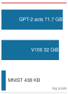
Activation memory spans MNIST toys to GPT-scale training.
Activation memory requirements
Training systems retain intermediate values requested by backward rules. The exact saved set depends on the operation, fusion, and recomputation strategy. Training state includes several distinct categories:
- saved forward values needed by backward rules,
- model parameters,
- parameter gradients, and
- optimizer state and any higher-precision parameter copies.
Consider a batch of training examples passing through a network. The forward pass computes and stores: \[\begin{gather*} \mathbf{Z}^{(\ell)} = \mathbf{A}^{(\ell-1)}\mathbf{W}^{(\ell)} + \mathbf{b}^{(\ell)} \\ \mathbf{A}^{(\ell)} = f(\mathbf{Z}^{(\ell)}) \end{gather*}\]
A conventional implementation may retain \(\mathbf{Z}^{(\ell)}\), \(\mathbf{A}^{(\ell)}\), or other inputs and outputs according to the derivative rule. Fused kernels and recomputation can retain a smaller set. Batch-dependent activations still create multiplicative pressure, while optimizer overhead scales with parameter count. The GPT-2 calculation decomposes that pressure into per-layer attention, feed-forward, and training-state costs.
Napkin Math 1.3: GPT-2 activation memory breakdown
For GPT-2 with batch size \(B\) = 4, sequence length \(S\) = 1024, hidden dimension \(d\) = 1600, and 48 layers:
Math:
- Attention activations: \(B \times S \times d \times 4\) (Q, K, V, output) = 4 \(\times\) 1024 \(\times\) 1600 \(\times\) \(4 \times 2\) bytes (FP16) = 52.4 MB
- FFN activations: \(B \times S \times (4d)\) (intermediate expansion) = 4 \(\times\) 1024 \(\times\) 6400 \(\times\) 2 bytes = 52.4 MB
- Attention scores: \(5 \times N_{\text{heads}} \times S^2 \times B\) bytes for the \(S{\times}S\) score, softmax, and dropout buffers. With 25 heads, this term reaches 524.3 MB per layer—the dominant term, quadratic in sequence length, and exactly what selective recomputation discards
- Layer norm states: Minimal (~10 MB per layer)
- Total per layer: ~639.1 MB (attention + FFN + attention scores + layer norm states)
Result:
- Total activation memory (library estimate, includes residual-stream and framework buffers beyond the line items above): 35.9 GB
- Parameters (FP16): 3 GB
- Gradients: 3 GB
- Master weights (FP32): 6 GB
- Adam moment state (FP32): 12 GB
- Peak memory during training: ~59.9 GB
This exceeds a single V100’s 32 GB capacity.
Solutions:
- Selective activation recomputation: Discard attention intermediates and recompute them during backward, reducing this modeled activation term by 70.2 percent to ~10.7 GB; the additional work depends on the implementation
- Activation CPU offloading: Store some activations in CPU RAM, transfer during backward pass
- Mixed precision: FP16 activations (already applied) vs. FP32 (would be 71.7 GB)
- Reduced micro-batch size and gradient accumulation: Build a larger effective batch from multiple memory-feasible forward/backward passes
Systems insight: Even after selective recomputation, the modeled activations plus static state total about 34.7 GB, slightly above the raw 32 GB V100 capacity before workspace and allocator overhead. Full recomputation, sharding, offload, or a smaller micro-batch is therefore still required for this representation.
This breakdown illustrates the practical engineering decisions required when accelerator memory falls short. The same trade-off between stored activations, recomputation, and batch size drives the memory-computation analysis that follows.
Checkpoint 1.2: The memory-compute trade-off
Training large models requires managing the memory wall (the bandwidth bottleneck introduced in Neural Computation and revisited in Why execution strategy matters: The memory wall).
Bottleneck
Scaling limits
Memory-computation trade-offs
Training systems must balance memory usage against computational efficiency. Each forward pass generates values that backward rules may request. For a simplified network model with \(N_L\) layers, let \(s_\ell\) denote the bytes of saved intermediate state per example at layer \(\ell\) and \(a_\ell\) the bytes of saved activation outputs per example. Under this per-example convention, their storage scales linearly with batch size and is approximated by equation 5:
\[ \text{Memory per batch} = B \times \sum_{\ell=1}^{N_L} (s_\ell + a_\ell) \tag{5}\]
This memory requirement compounds with the weights, gradients, and optimizer memory discussed in section 1.2.2.3. Equation 6 gives a conceptual training-state decomposition: \[ \text{Total Memory} = \text{Memory}_{\text{weights}} + \text{Memory}_{\text{gradients}} + \text{Memory}_{\text{optimizer}} + \text{Memory per batch} \tag{6}\]
The runtime peak can exceed this sum because temporary workspaces, communication buffers, allocator behavior, and framework bookkeeping also occupy memory. To reduce the activation term, training systems can strategically recompute intermediate values during backward rather than storing them. This increases computational work but can enable deeper networks or larger batches on memory-constrained hardware (Chen et al. 2016). Algorithm 2 makes the trade explicit: the forward pass keeps activations at only a sparse set of checkpoint layers, and the backward pass recomputes the rest on demand.
\begin{algorithm} \caption{Gradient checkpointing (activation recomputation)} \begin{algorithmic} \Require $N_L$-layer network; checkpoint set $\mathcal{C} \subseteq \{1,\dots,N_L\}$ (e.g., every $\sqrt{N_L}$ layers) \Ensure parameter gradients, at reduced peak activation memory \For{$\ell = 1$ to $N_L$} \State forward layer $\ell$; store its activation only if $\ell \in \mathcal{C}$ \Comment{drop the rest} \EndFor \For{$\ell = N_L$ down to $1$} \If{the activation of layer $\ell$ was dropped} \State recompute the forward segment from the nearest stored checkpoint through layer $\ell$ \EndIf \State compute the layer's gradient; free the activation \EndFor \State \Return the accumulated gradients \end{algorithmic} \end{algorithm}
If we space checkpoints every \(\sqrt{N_L}\) layers, we can reduce peak activation memory from \(\mathcal{O}(N_L)\) to \(\mathcal{O}(\sqrt{N_L})\) by doing extra forward work over checkpoint segments during the backward pass. That is the lever that fits a network too large to train within accelerator memory, trading the iron law’s operation term for activation capacity.
The efficiency of these memory management strategies depends heavily on the underlying hardware architecture. Accelerator systems, with their high computational throughput but limited memory bandwidth, often encounter different bottlenecks than CPU systems. Memory bandwidth limitations on accelerators mean that even when sufficient storage exists, moving data between memory and compute units can become the primary performance constraint (Jouppi et al. 2017).
Jouppi, Norman P., Cliff Young, Nishant Patil, David Patterson, Gaurav Agrawal, Raminder Bajwa, Sarah Bates, et al. 2017. “In-Datacenter Performance Analysis of a Tensor Processing Unit.” Proceedings of the 44th Annual International Symposium on Computer Architecture, ISCA ’17, 1–12. https://doi.org/10.1145/3079856.3080246.
Paszke, Adam, Sam Gross, Francisco Massa, Adam Lerer, James Bradbury, Gregory Chanan, Trevor Killeen, et al. 2019. “PyTorch: An Imperative Style, High-Performance Deep Learning Library.” Advances in Neural Information Processing Systems (NeurIPS) 32: 8024–35.
These hardware considerations guide the implementation of backpropagation in modern training systems. Specialized memory-efficient algorithms for operations like convolutions compute gradients in tiles or chunks, adapting to available memory bandwidth. Dynamic memory management tracks the lifetime of intermediate values throughout the computation graph, deallocating memory as soon as tensors become unnecessary for subsequent computations (Paszke et al. 2019).
Forward propagation, gradient computation, and parameter updates define what training systems must compute. An operation’s name alone, however, does not reveal where the system stalls. Matrix shape, fusion, precision, implementation, and hardware determine whether computation or data movement is binding. Arithmetic intensity provides the next analytical tool.
Arithmetic intensity
Arithmetic intensity captures this distinction—the ratio of computation to data movement that reveals whether an operation is limited by compute throughput or memory bandwidth: \[ \text{Arithmetic Intensity} = \frac{\text{FLOPs}}{\text{bytes moved}} \]
Operations with high arithmetic intensity are compute bound: their performance is limited by the processor’s computational throughput. Operations with low arithmetic intensity are memory bound: they spend more time moving data than computing. The Roofline model gives the formal definition of the Roofline Model and shows how to compute a hardware’s ridge point.17
17 Ridge point and precision: The roofline ridge point—the arithmetic intensity threshold separating memory-bound from compute-bound operations—shifts with numerical precision. On the same accelerator, a lower-precision Tensor Core path can expose much more arithmetic throughput at roughly the same memory bandwidth, raising the ridge point substantially. Switching from TF32-style execution to BF16 mixed precision can therefore change which optimization technique yields returns, making precision selection inseparable from roofline analysis.
Table 5 summarizes common tendencies rather than fixed measurements. Dense matrix multiplication can reuse operands enough to reach high arithmetic intensity, while standalone elementwise and reduction kernels often perform less work per byte moved. The target hardware’s ridge point determines the resulting regime.
| Operation | Arithmetic-intensity tendency | Classification condition |
|---|---|---|
| Dense MatMul (large) | High when shapes and tiling provide substantial operand reuse | Compute-bound only when intensity exceeds the ridge |
| Activation functions | Usually low as standalone elementwise kernels | Often memory-sensitive unless fusion removes traffic |
| LayerNorm/BatchNorm | Reduction and elementwise work with multiple tensor passes | Depends on fusion, shape, and target ridge point |
| Attention softmax | Reduction and normalization over the attention axis | Depends on materialization, tiling, and fusion |
Hardware efficiency during model training depends directly on kernel arithmetic intensity. Locate the operation points in figure 2 along the logarithmic arithmetic intensity axis, comparing memory-bandwidth bound operators on the sloped ceiling against compute-bound operators on the flat peak.
To build intuition for these relationships, study the roofline diagram in figure 2. The ridge point marks the “knee” where the sloped memory-bound region meets the flat compute-bound ceiling. An implementation plotted left of this point is bandwidth bound under the roofline assumptions; one plotted right is compute bound. The operation points in this diagram are illustrative placements that show how to interpret the model, not measured GPT-2 coordinates.
Consider a GPT-2 attention layer that materializes the \(S{\times}S\) attention-score matrix. For each head, the \(\mathbf{Q}\mathbf{K}^\top\) product costs approximately \(2S^2d_{\text{head}}\) FLOPs, while writing the FP16 score matrix and reading it back moves about \(4S^2\) bytes. Counting only that score-matrix traffic gives the approximation \(d_{\text{head}}/2\). For GPT-2 Small (\(d_{\text{model}}=\) 768 across 12 heads, so \(d_{\text{head}}=\) 64), this restricted accounting yields 32 FLOP/byte. A complete kernel analysis must also count Q and K traffic, softmax work, additional reads and writes, cache reuse, and fusion. The \(\mathcal{O}(S^2)\) materialized score traffic remains the term that FlashAttention targets.
Accelerators have characteristic hardware ridge points where operations transition from memory-bound to compute bound. A representative data-center accelerator has a ridge point high enough that low-intensity operations such as materialized attention softmax remain memory bound even when large matrix multiplications are compute bound. Operations below the ridge point are memory bound; above it, they are compute bound.
Systems Perspective 1.5: Peak FLOP/s vs. sustained performance
Peak TFLOP/s is an arithmetic ceiling rather than a prediction of sustained application performance. For an implementation that is strictly bandwidth bound, raising only the arithmetic ceiling does not improve the roofline bound. Mixed-precision training can both enable faster arithmetic paths and reduce traffic for tensors actually stored and transferred at lower precision. The realized gain depends on kernel support, conversion overhead, numerical requirements, and which resource is binding. Roofline-guided optimization therefore measures the implementation before choosing fusion, precision changes, or additional compute.
Batch size can influence arithmetic intensity and occupancy by changing matrix shapes and the amount of reuse available to a kernel. No universal boundary at batch 32 separates memory-bound from compute-bound execution; the transition depends on the operation, dimensions, implementation, precision, and hardware.
This analysis guides optimization strategy selection. For memory-bound operations, reducing data movement through operator fusion, reduced precision, or algorithmic improvements like FlashAttention provides the largest gains. For compute-bound operations, increasing throughput through Tensor Cores and parallel execution matters more. The distinction is practical: the first case asks how to move fewer bytes, while the second asks how to keep more arithmetic units busy.
In figure 2, FlashAttention18 captures the core insight of IO-aware algorithm design. By never materializing the full \(S{\times}S\) attention matrix in HBM and instead processing tiles that fit in fast SRAM, FlashAttention reduces auxiliary attention memory from \(\mathcal{O}(S^2)\) to \(\mathcal{O}(S)\) and sharply reduces HBM traffic. The original work reports up to 3\(\times\) speedups on evaluated workloads (Dao et al. 2022), with gains depending on tensor shape, hardware, and baseline. The algorithm and the conditions under which it applies are examined in detail in section 1.5.4.
18 FlashAttention: The core mechanism processes attention in small tiles that fit within the accelerator’s fast on-chip SRAM, avoiding writes of the full intermediate \(S{\times}S\) matrix to slower HBM. The exact HBM IO bound depends on tile size and SRAM capacity, but the practical effect is a large reduction in memory traffic and auxiliary activation storage. The original work reports workload-dependent speedups of up to 3\(\times\).
The arithmetic-intensity analysis in this section shows how to determine which resource constrains a particular implementation. Dense matrix multiplication often reaches the compute-bound regime when shapes provide enough reuse, while standalone normalization and activation kernels are often memory-sensitive. FlashAttention exemplifies how an algorithm can reduce data movement and raise arithmetic intensity, though the final regime remains workload dependent.
Optimizing individual operations is necessary but insufficient. A perfectly tuned matrix multiplication achieves nothing if the accelerator sits idle waiting for the next batch of data. The mathematical foundations established earlier in this chapter quantified the cost of each piece—matrix multiplications consuming trillions of FLOPs, activation functions bottlenecked by memory bandwidth, optimizer states tripling memory requirements. The next question is how to orchestrate these pieces into a pipeline where no stage starves the others.
Self-Check: Question
Why do batched matrix-matrix multiplications (GEMM, BLAS Level 3) dominate accelerator-based neural network training workloads, whereas matrix-vector operations (GEMV, BLAS Level 2) struggle to achieve high hardware utilization?
- Matrix-matrix operations avoid computing gradients during backpropagation, halving the memory footprint.
- Batched matrix-matrix operations exhibit \(\mathcal{O}(N)\) arithmetic intensity, allowing high operand reuse in on-chip SRAM/registers to saturate compute units, whereas matrix-vector operations have \(\mathcal{O}(1)\) arithmetic intensity and are strictly memory-bandwidth bound.
- Matrix-vector operations cannot be executed on GPUs without constant CPU synchronization barriers at every layer.
- Batched matrix-matrix operations reduce total model parameters, fitting larger architectures into accelerator HBM.
A team trains a 7-billion-parameter model on accelerators with 80 GB of HBM each. Weights, gradients, and activations together occupy 64 GB per accelerator at the planned batch size. Using the section’s optimizer-memory accounting, explain the systems trade-off between choosing standard SGD and Adam for this run.
The point on a roofline model curve where the memory-bandwidth-bound diagonal ceiling intersects the flat peak-compute ceiling, defined mathematically as \(\text{Peak FLOP/s} / \text{Memory Bandwidth}\), is known as the ____ point.
Order the following events in a standard backpropagation training step to reflect their strict causal and data dependencies:
- Compute scalar objective loss by evaluating predictions against ground-truth labels.
- Update model parameters using gradient-based optimization rules (such as Adam or SGD).
- Execute forward propagation through successive layers while caching intermediate activations.
- Evaluate the chain rule backward from the loss through layers to compute parameter and activation gradients.
- Fetch and preprocess the training mini-batch on the host and transfer it to device memory.
For a transformer with hidden dimension \(d_{\text{model}} = 768\) and 12 heads (\(d_{\text{head}} = 64\)), the arithmetic intensity of materialized attention score computation (\(\mathbf{Q}\mathbf{K}^\top\) and score matrix I/O) is approximately \(d_{\text{head}}/2 = 32\text{ FLOP/byte}\). If executed on an accelerator with a ridge point of \(153\text{ FLOP/byte}\), how does this kernel behave, and what optimization strategy is appropriate?
- The kernel is compute-bound; upgrade to an accelerator with higher peak TFLOP/s to accelerate execution.
- The kernel is latency-bound; reduce the batch size to 1 so the matrix fits in registers.
- The kernel is network-bound; upgrade the inter-node InfiniBand fabric to prevent AllReduce stalls.
- The kernel is memory-bandwidth bound because \(32 < 153\text{ FLOP/byte}\); apply IO-aware tiling (such as FlashAttention) to avoid writing and reading intermediate score matrices from HBM, increasing arithmetic intensity.
Pipeline Architecture
A training step is not a single operation but a sequence of dependent stages—data must be loaded before computation can begin, forward passes must complete before backward passes start, and gradients must be computed before parameters can update. The speed of the slowest stage determines the speed of the entire system.
The system-level pipeline coordinates these stages across real hardware with finite memory and bandwidth constraints. ML Frameworks introduced how frameworks like PyTorch and TensorFlow provide APIs for defining models and executing forward passes; here those API calls become part of a larger architecture of data loading, preprocessing, accelerator transfers, and parameter updates—a unified pipeline rather than isolated operations.
This orchestration is not a single monolithic process but rather three interconnected subsystems, each with distinct responsibilities and resource demands. Figure 3 traces how these subsystems connect: the data pipeline handles ingestion and preprocessing, the training loop executes forward passes, backward passes, and parameter updates, and the evaluation pipeline periodically assesses model quality. The flow between these components is where bottlenecks emerge—the interconnection points expose the binding constraints.
\begin{tikzpicture}[line join=round,
    font=\small\sffamily,
    box/.style={
        draw=none,%BlueLine,
        fill=none,%BlueL,
        rounded corners=2pt,
        align=center,
        minimum height=1.4cm,
        minimum width=3.2cm,
        line width=0.75pt,
        font=\small\sffamily
    },
    arrow/.style={
        ->,
        color=GrayLine,
        line width=1.0pt,
        >=latex
    },
    label_text/.style={
        font=\footnotesize\sffamily,
        align=center,
        color=TextBlack
    },
    node distance=2.0cm,
satellite/.style = {circle, draw=none, semithick, fill=#1,
                    text width=26mm, inner sep=1pt, align=flush center,
                    minimum size=28mm,minimum height=12mm},
arr/.style = {-{Triangle[length=5mm,width=2mm]}, color=#1,
                    line width=1mm, shorten <=1mm, shorten >=1mm},
]

%graph style
\tikzset{
pics/graph/.style = {
        code = {
        \pgfkeys{/channel/.cd, #1}
\begin{scope}[local bounding box=GRAPH,scale=1, every node/.append style={transform shape}]
\def\dx{\Width}
\def\dy{\Height}
\def\dz{\Depth}
% koordinata donjeg levog ugla (početak bara)
\def\x{0}
\def\y{0.15}
\def\z{0}
% boje
\draw[draw=\filllcirclecolor,line width=1pt](-0.2,0)--(1.3,0);
\draw[draw=\filllcirclecolor,line width=1pt](-0.2,0)--(-0.2,1.2);
\filldraw[fill=\filllcolor!10, draw=\drawcolor] (\x,\y+\dy,\z) -- (\x,\y+\dy,\z+\dz) -- (\x+\dx,\y+\dy,\z+\dz) -- (\x+\dx,\y+\dy,\z) -- cycle; % gornja strana
\filldraw[fill=\filllcolor!50, draw=\drawcolor] (\x+\dx,\y,\z) -- (\x+\dx,\y,\z+\dz) -- (\x+\dx,\y+\dy,\z+\dz) -- (\x+\dx,\y+\dy,\z) -- cycle; % desna strana
\filldraw[fill=\filllcolor!60, draw=\drawcolor] (\x,\y,\z+\dz) -- (\x+\dx,\y,\z+\dz) -- (\x+\dx,\y+\dy,\z+\dz) -- (\x,\y+\dy,\z+\dz) -- cycle; % prednja strana
\end{scope}
    }
  }
}
%brain
\tikzset{pics/brain/.style = {
        code = {
        \pgfkeys{/channel/.cd, #1}
\begin{scope}[local bounding box=BRAIN,scale=\scalefac, every node/.append style={transform shape}]
\draw[fill=\filllcolor,line width=\Linewidth](-0.3,-0.10)to(0.08,0.60)
to[out=60,in=50,distance=3](-0.1,0.69)to[out=160,in=80](-0.26,0.59)to[out=170,in=90](-0.46,0.42)
to[out=170,in=110](-0.54,0.25)to[out=210,in=150](-0.54,0.04)
to[out=240,in=130](-0.52,-0.1)to[out=300,in=240]cycle;
\draw[fill=\filllcolor,line width=\Linewidth]
(-0.04,0.64)to[out=120,in=0](-0.1,0.69)(-0.19,0.52)to[out=120,in=330](-0.26,0.59)
(-0.4,0.33)to[out=150,in=280](-0.46,0.42)
%
(-0.44,-0.03)to[bend left=30](-0.34,-0.04)
(-0.33,0.08)to[bend left=40](-0.37,0.2) (-0.37,0.12)to[bend left=40](-0.45,0.14)
(-0.26,0.2)to[bend left=30](-0.24,0.13)
(-0.16,0.32)to[bend right=30](-0.27,0.3)to[bend right=30](-0.29,0.38)
(-0.13,0.49)to[bend left=30](-0.04,0.51);
\draw[rounded corners=0.8pt,\drawcircle,-{Circle[fill=\filllcolor,length=7.5pt]},line width=\Linewidth](-0.23,0.03)--(-0.15,-0.03)--(-0.19,-0.18)--(-0.04,-0.28);
\draw[rounded corners=0.8pt,\drawcircle,-{Circle[fill=\filllcolor,length=7.5pt]},line width=\Linewidth](-0.17,0.13)--(-0.04,0.05)--(-0.06,-0.06)--(0.14,-0.11);
\draw[rounded corners=0.8pt,\drawcircle,-{Circle[fill=\filllcolor,length=7.5pt]},line width=\Linewidth](-0.12,0.23)--(0.31,0.0);
\draw[rounded corners=0.8pt,\drawcircle,-{Circle[fill=\filllcolor,length=7.5pt]},line width=\Linewidth](-0.07,0.32)--(0.06,0.26)--(0.16,0.33)--(0.34,0.2);
\draw[rounded corners=0.8pt,\drawcircle,-{Circle[fill=\filllcolor,length=7.5pt]},line width=\Linewidth](-0.01,0.43)--(0.06,0.39)--(0.18,0.51)--(0.31,0.4);
\coordinate(PO)at(-0.1,0.2);
\node[circle,draw=white,line width=1pt,fill=\filllcirclecolor,minimum size=5mm,inner sep=0pt](LV)at(PO){};
\node[draw=none,rotate=40,rounded corners=3pt,rectangle,minimum width=1.2mm,inner sep=1pt,
fill=\filllcirclecolor,minimum height=6mm,anchor=north]at(PO){};
\node[circle,draw=none,fill=white,minimum size=3.0mm,inner sep=0pt](LM)at(PO){};
\node[font=\tiny\bfseries]at(LM){...};
\end{scope}
     }
  }
}
%data
\tikzset{mycylinder/.style={cylinder, shape border rotate=90, aspect=1.3, draw, fill=white,
minimum width=25mm,minimum height=11mm,line width=\Linewidth,node distance=-0.15},
pics/data/.style = {
        code = {
        \pgfkeys{/channel/.cd, #1}
\begin{scope}[local bounding box=STREAMING,scale=\scalefac, every node/.append style={transform shape}]
\node[mycylinder,fill=\filllcolor!50] (A) {};
\node[mycylinder, above=of A,fill=\filllcolor!30] (B) {};
\node[mycylinder, above=of B,fill=\filllcolor!10] (C) {};
 \end{scope}
     }
  }
}
%%%
\pgfkeys{
  /channel/.cd,
  Depth/.store in=\Depth,
  Height/.store in=\Height,
  Width/.store in=\Width,
  filllcirclecolor/.store in=\filllcirclecolor,
  filllcolor/.store in=\filllcolor,
  drawcolor/.store in=\drawcolor,
  drawcircle/.store in=\drawcircle,
  scalefac/.store in=\scalefac,
  Linewidth/.store in=\Linewidth,
  picname/.store in=\picname,
 tiecolor/.store in=\tiecolor,
  bodycolor/.store in=\bodycolor,
  stetcolor/.store in=\stetcolor,
  tiecolor=red,      % default tie color
  bodycolor=blue!30,  % default body color
  stetcolor=green,  % default stet color
  filllcolor=BrownLine,
  filllcirclecolor=violet!20,
  drawcolor=black,
  drawcircle=violet,
  scalefac=1,
  Linewidth=0.5pt,
  Depth=0.2,
  Height=0.5,
  Width=0.25,
  picname=C
}

%training Loop
\node (s1) [satellite=magenta!90!black!10] at (0,0) {};
\pic[shift={(0.2,-0.3)}] at  (s1){brain={scalefac=1.7,picname=1,
filllcolor=orange!30!, filllcirclecolor=cyan!55!black!60, Linewidth=1.5pt}};
\node[box, below=1pt of s1] (s1t) {Training Loop\\
\footnotesize\sffamily Forward Pass, Loss,\\Backward Pass};
%Data pipeline
\node (s2) [satellite=brown!90!black!15] at (-6.65,0) {};
\pic[shift={(0.05,-0.55)}] at  (s2){data={scalefac=0.5,picname=1,filllcolor=BlueLine,
Linewidth=1.0pt}};
\node[box, below=1pt of s2] (data) {Data Pipeline\\
\footnotesize\sffamily Ingestion, Preprocessing,\\Batching};
%Evaluation
\node (s3) [satellite=cyan!20] at (6.65,0) {};
%graph
\begin{scope}[local bounding box=GRAPH1,shift={($(s3)+(-0.55,-0.6)$)},scale=1.2, every node/.append style={transform shape}]
\pic[shift={(0,0)}] at  (0,0){graph={filllcirclecolor=black!60,scalefac=0.5,picname=1,drawcolor=black,filllcolor=red,Height=0.5,Linewidth=1.25pt}};
\pic[shift={(0.33,0)}] at  (0,0){graph={filllcirclecolor=none,scalefac=0.5,picname=2,drawcolor=black,filllcolor=red,Height=1,Linewidth=1.25pt}};
\pic[shift={(0.66,0)}] at  (0,0){graph={filllcirclecolor=none,scalefac=0.5,picname=3,drawcolor=black,filllcolor=red,Height=0.25,Linewidth=1.25pt}};
\pic[shift={(0.99,0)}] at  (0,0){graph={filllcirclecolor=none,scalefac=0.5,picname=4,drawcolor=black,filllcolor=red,Height=0.75,Linewidth=1.25pt}};
\end{scope}
\node[box, below=1pt of s3] (eval) {Evaluation Pipeline\\
\footnotesize\sffamily Validation and Metrics};

\draw[arr=cyan,shorten >=1pt] (s2) --coordinate[pos=0.45](AR1) (s1);
\draw[arr=cyan,shorten >=1pt] (s1.10) --coordinate[pos=0.45](AR2) (s3.170);
\draw[arr=green!70!black,shorten >=1pt] (s3.190) --coordinate[pos=0.45](AR3) (s1.350);
% Data -> Training (top arrow)
\node[label_text,above=5pt of AR1]{Processed Batches};
% Training -> Evaluation (top arrow, shifted up)
\node[label_text,above=5pt of AR2]{Evaluation Metrics};
% Evaluation -> Training (bottom arrow, feedback)
\node[label_text,below=5pt of AR3]{Feedback};
\end{tikzpicture}Architectural overview
A single training iteration involves three subsystems executing in sequence: a data pipeline that ingests, transforms, and batches raw data; a training loop that performs the forward pass, gradient computation, and parameter update; and an evaluation pipeline that measures model quality against held-out data. This subsystem sequence frames the chapter’s training pipeline. Understanding each subsystem’s role clarifies where performance bottlenecks arise and where system-level optimizations have their greatest impact.
A training system is easiest to reason about from its boundaries inward. The data pipeline loads raw records from storage, applies transformations such as resizing, augmentation, and normalization, and assembles the resulting examples into batches; input normalization is a long-standing training aid (LeCun et al. 2012). The evaluation pipeline sits at the other boundary. At configurable intervals, it runs held-out validation data through the current model, computes metrics such as accuracy or loss, and exposes convergence problems such as overfitting, where training loss improves while validation loss degrades. Because evaluation consumes accelerator time, its cadence trades finer-grained feedback against training throughput.
LeCun, Yann, Leon Bottou, Genevieve B. Orr, and Klaus-Robert Müller. 2012. “Efficient BackProp.” In Neural Networks: Tricks of the Trade, vol. 7700, 7700. Lecture Notes in Computer Science. Springer Berlin Heidelberg. https://doi.org/10.1007/978-3-642-35289-8_3.
The core engine of neural network learning sequences forward predictions, backward error propagation, and parameter optimization into a closed loop. Follow the cyclic data path in figure 4 across the three sequential stages: forward pass, gradient calculation, and weight updates.
\begin{tikzpicture}[
    box/.style 2 args={
        draw=#2,
        fill=#1,
        rounded corners=0pt,
        align=center,
        minimum height=10mm,
        minimum width=22mm,
        line width=0.75pt,
        font=\footnotesize\sffamily
    },
    box_lg/.style 2 args={
        box={#1}{#2},
        minimum width=22mm
    },
    box_blue/.style ={
        box={BlueL}{BlueLine},
        minimum width=25mm
    },
    arrow/.style={
        ->,
        color=GrayLine,
        line width=1.2pt,
        >=latex
    },
    dash_arrow/.style={
        arrow,
        dashed
    },
    node distance=1.4cm and 1.9cm
]

% Row 1: Predict
\node[box={GreenL}{GreenLine}] (batch) {Training\\Batch};
\node[box_blue, right=of batch] (forward) {Forward Pass\\(Model)};
\node[box={GreenL}{GreenLine}, right=of forward] (pred) {Predicted\\Labels};
% Row 2: Gradients
\node[box_lg={RedL}{RedLine}, below=8mm of pred] (loss) {Loss Function\\(Error Calculation)};
\node[box_blue, below=8mm of forward] (grads) {Backward Pass\\(Chain Rule)};
\node[box={GreenL}{GreenLine}, below=8mm of batch] (backward) {Parameter\\Gradients};
%labels
\node[box={GreenL}{GreenLine}, right=of loss] (truth) {Ground\\Truth};
\node[above=0.1cm of truth, font=\footnotesize\sffamily\itshape, color=gray] {Labels};
% Row 3: Update
\node[box_lg={OrangeL}{OrangeLine}, below=8mm of backward] (optim) {Optimizer\\(Adam/SGD)};
\node[box_blue, below=8mm of grads] (update) {Update\\Parameters};
% Connections
\draw[arrow] (batch) -- (forward);
\draw[arrow] (forward) -- (pred);
\draw[arrow] (pred) -- (loss);
\draw[dash_arrow] (truth) -- (loss);
\draw[arrow] (loss) -- (grads);
\draw[arrow] (grads) -- (backward);
\draw[arrow] (backward) -- (optim);
\draw[arrow] (optim) -- (update);
% Updated parameters feed the model, while each new batch remains a separate input.
\draw[dash_arrow] (update.east) -- ++(0.5,0) coordinate(a)
    -- (a |- optim.south) -- ++(0,-0.35) coordinate(b)
    node[right, font=\footnotesize\sffamily\itshape,
color=gray, pos=0] {Next Iteration}
    -- (b -| backward.west) -- ++(-0.8,0) coordinate(c)
    -- (c |- batch.south) -- ++(0,-0.10) coordinate(d)
    -- (d -| forward.south) -- (forward.south);
% Step labels
\node[above=1pt of forward, font=\small\sffamily\bfseries, color=TextBlack] {Step 1: Predict};
\node[above=1pt of grads, font=\small\sffamily\bfseries, color=TextBlack] {Step 2: Gradients};
\node[above=1pt of $(optim.north east)!0.5!(update.north west)$,
font=\small\sffamily\bfseries, color=TextBlack] {Step 3: Update};
\end{tikzpicture}Each iteration executes the forward pass, loss computation, backward pass, and parameter update cycle established in section 1.2. The systems question is not what these operations compute (covered earlier) but how they interact as a pipeline, where the bottleneck in any one stage limits overall throughput.
This process repeats across batches and epochs, gradually refining the model to improve its predictive accuracy. The loop is tightly coupled to the stages around it: data preparation can overlap with computation by preprocessing the next batch while the current batch trains, while evaluation temporarily pauses gradient updates to measure validation quality. The integration minimizes idle time for system resources, but any imbalance, such as a slow data pipeline or an overly frequent evaluation schedule, propagates as reduced overall throughput.
Data pipeline
The architectural overview identified the data pipeline as the first component in the training system. Its efficiency directly determines whether expensive accelerator resources remain fully engaged or sit idle waiting for data. The systems aspects of data movement and preprocessing are the focus here; the upstream data engineering practices are covered in Data Engineering.
The data pipeline running on the CPU bridges raw data storage and accelerator computation. Figure 5 breaks down this architecture into three distinct zones.
\begin{tikzpicture}[font=\small\sffamily, >=stealth]
\tikzset{
Box/.style={align=center, inner xsep=2pt,draw=GreenLine, line width=1pt,fill=none,
minimum width=27mm, minimum height=25mm,node distance=1.0},
LineA/.style={violet!50,line width=4.0pt,{-{Triangle[width=1.5*6pt,length=2.0*5pt]}},shorten <=1pt,shorten >=1pt},
ALine/.style={black!50, line width=1.1pt,{{Triangle[width=0.9*6pt,length=1.2*6pt]}-}},
Larrow/.style={fill=violet!50, single arrow,  inner sep=2pt, single arrow head extend=3pt,
            single arrow head indent=0pt,minimum height=10mm, minimum width=3pt},
Text2/.style={font=\sffamily\bfseries\small,align=center}
}

%file_transfer
\tikzset{
pics/fileT/.style = {
        code = {
        \pgfkeys{/channel/.cd, #1}
\begin{scope}[shift={($(0,0)+(0,0)$)},scale=\scalefac,every node/.append style={transform shape}]
\draw[fill=\filllcirclecolor,draw=\drawcolor,line width=\Linewidth](-0.53,0.8)--(-0.22,0.5)--(-0.22,-0.54)
arc[start angle=360, end angle=270, radius=1mm]
--(-1.18,-0.65)arc[start angle=270, end angle=180, radius=1mm]--  (-1.28,0.7)
 arc[start angle=180, end angle=90, radius=1mm]--(-0.53,0.8);
 \draw[draw=\drawcolor,line width=\Linewidth](-0.53,0.8)|-(-0.22,0.5);
%right
\draw[fill=\filllcolor,line width=\Linewidth,draw=\drawcolor](0.72,0.8)--(1.03,0.5)--(1.03,-0.54)
arc[start angle=360, end angle=270, radius=1mm]
--(0.07,-0.65)arc[start angle=270, end angle=180, radius=1mm]--  (-0.03,0.7)
 arc[start angle=180, end angle=90, radius=1mm]--(0.72,0.8);
 \draw[draw=\drawcolor,line width=\Linewidth](0.72,0.8)|-(1.03,0.5);
 %
 \fill[\filllcirclecolor,](-0.450,0)--(0.220,0)--(0.220,0.13)--(0.6220,-0.1)--(0.220,-0.33)--(0.220,-0.2)--(-0.32,-0.2);
\draw[draw=\drawcolor,line width=\Linewidth](-0.450,0)--(0.220,0)--(0.220,0.13)--(0.6220,-0.1)--(0.220,-0.33)--(0.220,-0.2)--(-0.32,-0.2);
\fill[\filllcolor](0.220,0)--(-0.450,0)--(-0.450,-0.13)--(-0.880,0.1)--(-0.450,0.33)--(-0.450,0.19)--(0.1,0.19);
\draw[draw=\drawcolor,line width=\Linewidth](0.220,0)--(-0.450,0)--(-0.450,-0.13)--(-0.880,0.1)--(-0.450,0.33)--(-0.450,0.19)--(0.1,0.19);
%
\end{scope}
    }
  }
}
%dataP
\tikzset{mycylinder/.style={cylinder, shape border rotate=90, aspect=1.3, draw, fill=white,
minimum width=25mm,minimum height=11mm,line width=\Linewidth,node distance=-0.15},
pics/dataP/.style = {
        code = {
        \pgfkeys{/channel/.cd, #1}
\begin{scope}[local bounding box=DATA,scale=\scalefac, every node/.append style={transform shape}]
\node[mycylinder,fill=\filllcolor!50] (A) {};
\node[mycylinder, above=of A,fill=\filllcolor!50] (B) {};
\node[mycylinder, above=of B,fill=\filllcolor!10] (C) {};
\fill[\filllcolor!50!black]($(C.west)!0.12!(C.east)$)circle(3pt);
\fill[\filllcolor!50!black]($(B.west)!0.12!(B.east)$)circle(3pt);
\fill[\filllcolor!50!black]($(A.west)!0.12!(A.east)$)circle(3pt);
%
\draw[draw=\drawcolor,line width=2.5*\Linewidth](B.east)--++(17mm,0);
\node[draw=\drawcolor,line width=\Linewidth,minimum width=9mm,fill=white,minimum height=22mm](BD)at($(B.east)+(8mm,0)$){};
\node[draw=\drawcolor,line width=\Linewidth,minimum width=5mm,minimum height=8mm,fill=white](BDM)at($(BD.east)+(5mm,0)$){};
\node[circle,draw=orange,line width=\Linewidth,minimum size=5mm]at($(BD.north)!0.2!(BD.south)$){};
\node[rectangle,draw=blue,line width=\Linewidth,minimum size=5mm]at($(BD.north)!0.5!(BD.south)$){};
\node[circle,draw=green,line width=\Linewidth,minimum size=5mm]at($(BD.north)!0.8!(BD.south)$){};
\end{scope}
     }
  }
}
%gear
\tikzset{
  pics/gear/.style args={#1/#2/#3/#4/#5/#6/#7}{
   code={
           \pgfkeys{/channel/.cd, #7}
\begin{scope}[shift={($(0,0)+(0,0)$)},scale=\scalefac,every node/.append style={transform shape}]
    \pgfmathtruncatemacro{\N}{#1}%
    \def\rin{#2}\def\rout{#3}\def\aA{#4}\def\aOff{#5}\def\rcut{#6}%
    \path[draw=\drawcolor,fill=\filllcolor]
      (0:\rin)
      \foreach \i [evaluate=\i as \n using (\i-1)*360/\N] in {1,...,\N}{%
        arc (\n:\n+\aA:\rin)
        -- (\n+\aA+\aOff:\rout)
        arc (\n+\aA+\aOff:\n+360/\N-\aOff:\rout)
        -- (\n+360/\N:\rin)
      } -- cycle;
      \draw[draw=none,fill=white](0,0) circle[radius=\rcut];
\end{scope}
  }}
}
%square-block
\tikzset{
pics/squareB/.style = {
        code = {
        \pgfkeys{/channel/.cd, #1}
\begin{scope}[line join=round,local bounding box=SQUARE,scale=\scalefac,every node/.append style={transform shape}]
% Right Face
\draw[fill=\filllcolor!70,line width=\Linewidth]
(\Depth,0,0)coordinate(\picname-ZDD)--(\Depth,\Width,0)--(\Depth,\Width,\Height)--(\Depth,0,\Height)--cycle;
% Front Face
\draw[fill=\filllcolor!40,line width=\Linewidth]
(0,0,\Height)coordinate(\picname-DL)--(0,\Width,\Height)coordinate(\picname-GL)--
(\Depth,\Width,\Height)coordinate(\picname-GD)--(\Depth,0,\Height)coordinate(\picname-DD)--(0,0,\Height);
% Top Face
\draw[fill=\filllcolor!20,line width=\Linewidth]
(0,\Width,0)coordinate(\picname-ZGL)--(0,\Width,\Height)coordinate(\picname-ZGL)--
(\Depth,\Width,\Height)--(\Depth,\Width,0)coordinate(\picname-ZGD)--cycle;
\end{scope}
    }
  }
}
%stackedS
\tikzset{%
 pics/stackedS/.style = {
        code = {
        \pgfkeys{/channel/.cd, #1}
\begin{scope}[local bounding box=FUNNEL,scale=\scalefac, every node/.append style={transform shape}]
%plats

\draw[fill=\filllcolor,line width=\Linewidth,draw=\drawcolor](0,-0.2)--(-0.67,0.13)--(0,0.47)--(0.67,0.13)--cycle;
\draw[fill=\filllcirclecolor,line width=\Linewidth,draw=\drawcolor](0,0)--(-0.67,0.33)--(0,0.67)--(0.67,0.33)--cycle;
\draw[fill=\filllcolor,line width=\Linewidth,draw=\drawcolor](0,0.2)--(-0.67,0.53)--(0,0.87)--(0.67,0.53)--cycle;
\draw[fill=\filllcirclecolor,line width=\Linewidth,draw=\drawcolor](0,0.4)--(-0.67,0.73)--(0,1.07)--(0.67,0.73)--cycle;
\end{scope}
     }
  }
}
%CPU2
\tikzset{%
 pics/cpu2/.style = {
        code = {
        \pgfkeys{/channel/.cd, #1}
\begin{scope}[local bounding box=CHIP,scale=\scalefac, every node/.append style={transform shape}]
\node[fill=\filllcolor,minimum width=15mm, minimum height=15mm,inner sep=0pt,
            rounded corners=2,outer sep=2pt] (C1) {};
\node[fill=white,minimum width=11mm, minimum height=11mm,inner sep=0pt,] (C2) {};
\node[fill=\filllcolor!40,minimum width=7mm, minimum height=7mm,inner sep=0pt,] (C3) {};
\foreach \x in {0.2,0.5,0.8}{
\draw[line width=2*\Linewidth,draw=\drawcolor,
-{Circle[fill=white,length=4.5pt]}]($(C1.north west)!\x!(C1.north east)$)--++(0,5mm);
}
\foreach \x in {0.2,0.5,0.8}{
\draw[line width=2*\Linewidth,draw=\drawcolor,
-{Circle[fill=white,length=4.5pt]}]($(C1.south west)!\x!(C1.south east)$)--++(0,-5mm);
}
\foreach \x in {0.2,0.5,0.8}{
\draw[line width=2*\Linewidth,draw=\drawcolor,
-{Circle[fill=white,length=4.5pt]}]($(C1.north west)!\x!(C1.south west)$)--++(-5mm,0);
}
\foreach \x in {0.2,0.5,0.8}{
\draw[line width=2*\Linewidth,draw=\drawcolor,
-{Circle[fill=white,length=4.5pt]}]($(C1.north east)!\x!(C1.south east)$)--++(5mm,0);
}
 \end{scope}
     }
  }
}
\pgfkeys{
  /channel/.cd,
  Depth/.store in=\Depth,
  Height/.store in=\Height,
  Width/.store in=\Width,
  filllcirclecolor/.store in=\filllcirclecolor,
  filllcolor/.store in=\filllcolor,
  drawcolor/.store in=\drawcolor,
  drawcircle/.store in=\drawcircle,
  scalefac/.store in=\scalefac,
  Linewidth/.store in=\Linewidth,
  picname/.store in=\picname,
  filllcolor=BrownLine,
  filllcirclecolor=cyan,
  drawcolor=black,
  drawcircle=violet,
  scalefac=1,
  Linewidth=0.5pt,
  Depth=1.3,
  Height=0.8,
  Width=1.1,
  picname=C
}

%Raw Data  (Disk/S3)
\node[Box](B1){};
%\fill[fill=none](B1.north west) rectangle ($(B1.north east)!0.6!(B1.south east)$)coordinate(B1DE);
\fill[green!20](B1.south east) rectangle ($(B1.north west)!0.6!(B1.south west)$)coordinate(B1LE);
\node[Box,draw=mygreen](){};
\node[Text2](T1)at($(B1.south east)!0.5!(B1LE)$){Raw Data \\(Disk/S3)};
\coordinate(Q1)at($(B1.north east)!0.5!(B1LE)$);
\pic[shift={(-0.35,-0.45)}] at  (Q1){dataP={scalefac=0.4,filllcirclecolor=violet!20,filllcolor=BlueLine, Linewidth=0.7pt}};
%Format Conversion
\node[Box, right=of B1](B2){};
\fill[cyan!20](B2.south east) rectangle ($(B2.north west)!0.6!(B2.south west)$)coordinate(B2LE);
\node[Box, right=of B1,draw=myblue](B2){};
\node[Text2]at($(B2.south east)!0.5!(B2LE)$){Format\\ Conversion};
\coordinate(Q2)at($(B2.north east)!0.5!(B2LE)$);
\pic[shift={(0.11,0)}] at  (Q2){fileT={scalefac=0.8,picname=1,drawcolor=black,
filllcolor=magenta!40,Linewidth=0.7pt, filllcirclecolor=white}};
%Preprocessing\\ (Augment)
\node[Box, right=of B2](B3){};
\fill[cyan!20](B3.south east) rectangle ($(B3.north west)!0.6!(B3.south west)$)coordinate(B3LE);
\node[Box, right=of B2,draw=myblue](B3){};
\node[Text2]at($(B3.south east)!0.5!(B3LE)$){Preprocessing\\ (Augment)};
\coordinate(Q3)at($(B3.north east)!0.5!(B3LE)$);
\pic[shift={(0,0)}] at (Q3) {gear={14/1.4/1.7/8/4/0.7/scalefac=0.35,drawcolor=mybrown,filllcolor=mybrown}};
%Batching
\node[Box, right=of B3](B4){};
\fill[cyan!20](B4.south east) rectangle ($(B4.north west)!0.6!(B4.south west)$)coordinate(B4LE);
\node[Box, right=of B3,draw=myblue](B4){};
\node[Text2]at($(B4.south east)!0.5!(B4LE)$){Batching};
\coordinate(Q4)at($(B4.north east)!0.5!(B4LE)$);
%\pic[rotate=0,shift={(-0.55,-0.5)}] at  (Q4){squareB={scalefac=0.5,picname=1,filllcolor=myblue, Linewidth=0.5pt}};
%\pic[rotate=0,shift={(0.1,-0.5)}] at  (Q4){squareB={scalefac=0.5,filllcolor=myblue, Linewidth=0.5pt}};
%\pic[rotate=0,shift={(-0.23,0.05)}] at  (Q4){squareB={scalefac=0.5,filllcolor=myblue, Linewidth=0.5pt}};
\pic[shift={(0,-0.450)}] at  (Q4){stackedS={scalefac=1,picname=1,Linewidth=1.0pt,
 filllcolor=cyan!90!black!40!,drawcolor=black,filllcirclecolor=myorange}};
%GPU 1
\node[Box, right=1.65 of B4](B5){};
\fill[fill=white](B5.north west) rectangle ($(B5.north east)!0.6!(B5.south east)$);
\fill[black!15](B5.south east) rectangle ($(B5.north west)!0.6!(B5.south west)$)coordinate(B5LE);
\node[Box, right=1.65of B4,draw=black](B5){};
\node[Text2]at($(B5.south east)!0.5!(B5LE)$){GPU 1};
\coordinate(Q5)at($(B5.north east)!0.5!(B5LE)$);
\pic[shift={(0.,0)}] at  (Q5){cpu2={scalefac=0.5, drawcolor=BlueLine, filllcolor=BlueLine, Linewidth=0.5pt}};
%
\begin{scope}[on background layer]
\node[Box, below right=1.6 and 0.6 of B5.north west](B5B){};
\fill[black!15](B5B.south east) rectangle ($(B5B.north west)!0.6!(B5B.south west)$)coordinate(B5LEB);
\node[Text2]at($(B5B.south east)!0.5!(B5LEB)$){GPU 3};
\node[Box, below right=1.6 and 0.6 of B5.north west,draw=black]{};
%%
\node[Box, below right=0.8 and 0.3 of B5.north west](B5A){};
\fill[fill=white](B5A.north west) rectangle ($(B5A.north east)!0.6!(B5A.south east)$);
\fill[black!15](B5A.south east) rectangle ($(B5A.north west)!0.6!(B5A.south west)$)coordinate(B5LEA);
\node[Text2]at($(B5A.south east)!0.5!(B5LEA)$){GPU 2};
\node[Box, below right=0.8 and 0.3 of B5.north west,draw=black]{};
\end{scope}
%arrows
\foreach \i in {1,2,3,4}{
\pgfmathtruncatemacro{\x}{\i + 1} %
\draw[LineA](B\i)--coordinate[pos=0.47](SR\i)(B\x);
}
\node[above=2pt of SR4]{Data};
%
\node[draw=mygreen,thick,inner sep=2mm,dashed,fit=(B1)](BB1){};
\node[below=0pt of BB1,mygreen]{Storage Zone};
\node[draw=myblue,thick,inner sep=2mm,dashed,fit=(B2)(B4)](BB2){};
\node[below=0pt of BB2,myblue]{CPU Preprocessing Zone};
%
\node[draw=black,thick,inner sep=2mm,dashed,fit=(B5)(B5A)(B5B)](BB3){};
\node[below=0pt of BB3,black]{GPU Training Zone};
\end{tikzpicture}These zones matter because each can become the slowest stage. Storage supplies raw examples from disk, typically image files for computer vision or text files for natural language processing. CPU preprocessing then converts formats, applies resizing, normalization, or data augmentation, and batches examples into tensors the accelerator can consume.
The GPU training zone consumes those preprocessed batches across multiple accelerators for parallel computation. Format conversion, processing, and batching are therefore not housekeeping steps; they are throughput gates. If any one runs slower than the training loop, expensive accelerator resources idle while the data pipeline catches up.
Core components
The data pipeline’s throughput is ultimately limited by how fast training data can be retrieved from storage. The data engineering practices from Data Engineering, including data format selection (Parquet, TFRecord, Arrow), partitioning strategies, and data locality optimization, directly impact these storage characteristics. These storage constraints propagate through the training system.
Storage throughput is bounded by the slower of two hardware constraints, expressed in equation 7: \[R_{\text{storage}} =\min(\text{BW}_{\text{disk}}, \text{BW}_{\text{network}}) \tag{7}\] where \(\text{BW}_{\text{disk}}\) is the physical disk bandwidth and \(\text{BW}_{\text{network}}\) represents the network bandwidth for distributed storage systems. In practice, training workloads rarely achieve this theoretical maximum because data shuffling can turn large sequential reads into smaller, less efficient accesses. Effective storage throughput can be modeled as \(R_{\text{storage,eff}} = R_{\text{storage}} \times F_{\text{access}}\), where \(F_{\text{access}}\) depends on record size, file layout, caching, and storage hardware. This penalty explains why data pipeline engineering matters: without careful layout, prefetching, and buffering, accelerators can sit idle waiting for storage.
Preprocessing
After storage, preprocessing turns raw inputs into model-ready tensors. Data pipelines from Data Engineering commonly extract and load raw data before transforming it on demand during training. Under ideal independent-worker scaling, preprocessing throughput grows with worker count as expressed in equation 8: \[R_{\text{preprocessing}} = \frac{N_{\text{workers}}}{T_{\text{transform}}} \tag{8}\] where \(N_{\text{workers}}\) parallel processing threads each perform transformations requiring \(T_{\text{transform}}\) seconds. Training architectures employ multiple workers to ensure preprocessing keeps pace with accelerator consumption rates—a single thread performing image augmentation at 30 ms per batch cannot feed an accelerator that computes a forward pass in 10 ms.
Preprocessed data must then transfer to the accelerator before computation can begin. The overall training throughput is therefore constrained by the slowest of three stages, as equation 9 makes explicit: \[R_{\text{training}} =\min\left(R_{\text{preprocessing}}, \frac{\text{BW}_{\text{GPU transfer}}}{D_{\text{vol}}^{(\text{batch})}}, \frac{R_{\text{compute}}}{O_{\text{batch}}}\right) \tag{9}\] where \(D_{\text{vol}}^{(\text{batch})}\) is the input bytes per batch and \(O_{\text{batch}}\) is the forward-backward work per batch in FLOPs. Every term is therefore expressed in batches per second before the minimum is taken.
Example 1.1: GPT-2 language model data pipeline
Scenario: Quantifying storage access, CPU tokenization, and PCIe host-to-device transfers supplying a 32-V100 GPU cluster training GPT-2.
Stage trace:
- Raw text storage: The WebText corpus contributes about 40 GB of raw text. Sequential reads from NVMe SSD storage reach 7 GB/s. Under document sampling with access factor 0.1, random-access storage bandwidth drops to 0.70 GB/s, giving \(T_{\text{read}} = D_{\text{vol}} / \text{BW}_{\text{storage}} \approx 0.1\text{ ms}\).
- Tokenization: A BPE tokenizer (50,257 vocabulary) converts text into token IDs. For batch size \(B =\) \(B=32\) and sequence length \(S =\) \(S=1024\) (32.8K tokens total), a single CPU core processing 500K tokens/s takes \(T_{\text{tokenize}} \approx\) 65.5 ms per batch.
- Batching and padding: Padding and packing generate an int64 tensor of shape 32 sequences \(\times\) 1,024 tokens, producing 262.1 KB per batch.
- PCIe transfer: Transferring the tensor across a PCIe Gen3 x16 bus (15.75 GB/s bandwidth) takes \(T_{\text{transfer}} =\) 0.017 ms, making bus transfer negligible.
Systems insight: Single-core CPU preparation (\(T_{\text{prep}} \approx\) 65.6 ms) consumes most of the accelerator step budget (\(T_{\text{step}} \approx\) 84.4 ms), so a serial pipeline pays both costs on every step and \(\eta_{\text{hw}}\) falls to about 56 percent. Push preparation any slower and the accelerator starves outright. Scaling to 8 parallel worker processes reduces tokenization latency to \(T_{\text{tokenize}} / N_{\text{worker}} \approx\) 8.2 ms, while prefetching overlaps \(T_{\text{prep}}\) with \(T_{\text{step}}\) to restore hardware utilization to 95 percent, delivering 379 global samples per second across 32 V100 GPUs.
This min-of-three relationship governs training pipeline design because system throughput equals bottleneck throughput. An accelerator with 312 TFLOP/s of compute capacity delivers zero useful work while waiting for data. Conversely, a perfectly optimized data pipeline provides no benefit if the accelerator is already compute-saturated. Balanced pipeline design aligns preprocessing capacity, transfer bandwidth, and compute throughput so that no single stage dominates iteration time. Applying this throughput analysis to the GPT-2 lighthouse model reveals where the data pipeline bottleneck lies for language model training.
Data pipeline throughput is not the only flow that can starve the accelerator. Multi-GPU training adds a second stream of traffic, the gradient synchronization required after every step, and once synchronization time exceeds compute time, communication becomes the limiting wall. Section 1.6.2 quantifies that network wall at the point where training crosses the node boundary.
System implications
The data pipeline and compute engine form a coupled system whose throughput equals the slower of the two, as equation 10 states: \[R_{\text{system}} =\min(R_{\text{pipeline}}, R_{\text{compute}}) \tag{10}\]
This relationship has direct consequences. When \(R_{\text{pipeline}} < R_{\text{compute}}\), the accelerator sits idle waiting for data, and accelerator utilization drops proportionally, as equation 11 shows: \[\text{Accelerator Utilization} = \min\left(1, \frac{R_{\text{pipeline}}}{R_{\text{compute}}}\right) \times 100\% \tag{11}\]
A ResNet-50 model on modern accelerator hardware can process 1,000 images per second, but if the data pipeline delivers only 200 images per second, accelerator utilization drops to 20 percent—the accelerator is idle 80 percent of the time. Upgrading to faster hardware does not help in this case; an accelerator capable of 2,000 images per second would achieve only 10 percent utilization with the same pipeline. Balanced system design aims to keep the accelerator supplied with data rather than waiting on an upstream stage.
Data flows
Training data traverses three memory tiers on its way from disk to accelerator, and the bandwidth gap between these tiers, spanning three orders of magnitude, is the central challenge of data pipeline design. The effective transfer rate through the hierarchy is bounded by its slowest link, as equation 12 shows: \[R_{\text{memory}} =\min(\text{BW}_{\text{storage}}, \text{BW}_{\text{system}}, \text{BW}_{\text{accelerator}}) \tag{12}\]
Bandwidth steps up the storage to DRAM to HBM hierarchy.
Local NVMe storage provides 7 GB/s, system memory delivers 50 GB/s, and accelerator HBM achieves 900 GB/s or higher. Each tier is roughly an order of magnitude faster than the one below it, which means data that flows freely within accelerator memory creates a severe bottleneck when it must be fetched from disk. This cascading bandwidth hierarchy explains why the iteration time of a well-pipelined system is governed by the maximum of its component latencies rather than their sum, as equation 13 shows: \[T_{\text{iteration}} =\max(T_{\text{fetch}}, T_{\text{process}}, T_{\text{transfer}}) \tag{13}\]
When pipeline stages overlap correctly (fetching the next batch from storage while preprocessing the current one and transferring the previous one to the accelerator), the iteration time equals the duration of the slowest stage rather than the sum of all stages. This overlap is exactly what prefetching achieves, turning a serial bottleneck into a parallel pipeline where each tier operates concurrently on different batches.
Practical architectures
An NVMe device rated at 7 GB/s would sustain 3.50 GB/s if a workload achieved half of peak. Small random reads and shuffling can reduce throughput further; the penalty depends on access size, queue depth, file layout, and caching.
To keep accelerators fed despite this bandwidth reduction, pipeline architectures maintain multiple data buffers simultaneously—prefetch buffers loading future batches, processing buffers holding data under transformation, and transfer buffers staging data for accelerator consumption. The total host memory required scales with the per-batch memory footprint \(M_{\text{batch}}\) according to equation 14: \[M_{\text{required}} = (N_{\text{prefetch}} + N_{\text{processing}} + N_{\text{transfer}}) \times M_{\text{batch}} \tag{14}\]
To avoid starving the accelerator, average preprocessing service time per batch must satisfy equation 15. \[T_{\text{preprocessing}} \leq T_{\text{compute}} \tag{15}\]
If preprocessing takes 40 ms per batch on one worker while the accelerator consumes one every 10 ms, ideal scaling requires at least four workers. Actual requirements depend on storage, CPU contention, and transformation cost; section 1.5.2 examines prefetching and parallel workers.
Forward pass
Prepared batches enter the training loop through the forward pass, where input data propagates through the model to generate predictions. The conceptual flow follows the layer-by-layer transformation \(\mathbf{A}^{(\ell)} = f\left(\mathbf{A}^{(\ell-1)}\mathbf{W}^{(\ell)} + \mathbf{b}^{(\ell)}\right)\) established earlier, but the system-level implementation must schedule kernels, move activations, and preserve enough state for backpropagation.
Compute operations
The forward pass orchestrates the computational patterns introduced in section 1.2.1.2, optimizing them for specific neural network operations. Building on the matrix multiplication foundations, the system must efficiently execute the \(N \times M \times B\) multiply-accumulate operations required for each layer, where typical layers with dimensions of \(512 \times 1024\) processing batches of 64 samples execute about 33.6 million MACs, or about 67.1 MFLOP under the two-FLOPs-per-MAC convention.
Systems Perspective 1.6: Wave quantization and tail effects
A common mistake in ML systems is ignoring the fixed execution granularity of GPU kernels. GPU execution is quantized into “waves” of work, but the relevant unit is the kernel’s thread or tile mapping, not necessarily one sample per thread.
Table 6: Illustrative Warp-Tail Arithmetic: Under a one-work-item-per-thread mapping, counts just above a 32-thread boundary launch a partially filled warp, so 33 items use two warps while 64 fill the same two warps. Actual training kernels map tensors to threads and tiles in implementation-specific ways, often assigning many threads to each sample, so these values cannot be inferred from batch size alone. Profiling must identify the kernel’s real mapping and wave boundaries.
The wave effect: An NVIDIA GPU executes work in warps of 32 threads. In the illustrative special case where one independent work item maps to one thread, 32 items fill one warp while 33 items require a second, mostly empty warp. Neural-network kernels usually map each sample to many threads, so batch size alone does not determine this utilization.
Tail effects at scale: On a large GPU like the H100 with 132 Streaming Multiprocessors (SMs), where each SM schedules groups of warps, the hardware can process thousands of threads in one “wave.” If the total workload is just slightly over a wave boundary (e.g., 1.01 waves), the hardware must wait for a nearly empty wave to finish before the next task begins.
Table 6 quantifies that one-item-per-thread illustration. It is not a general batch-size performance model.
| Independent Work Items | Warps Needed | Lane Utilization | Relative Time |
|---|---|---|---|
| 32 | 1 | 100% | 1\(\times\) |
| 33 | 2 | 51.6% | ~2× |
| 64 | 2 | 100% | 1\(\times\) |
| 65 | 3 | 67.7% | ~1.5× |
Engineering rule: Align tensor and tile dimensions with the kernel’s hardware mapping, then benchmark candidate batch sizes. A profiler can reveal partially filled warps or waves; batch size by itself cannot.
Understanding these tail effects is the difference between a practitioner who tunes by trial-and-error and an engineer who designs for the hardware.
Modern neural architectures extend beyond these basic matrix operations to include specialized computational patterns. Convolutional networks, for instance, perform systematic kernel operations across input tensors. Consider a typical input tensor of dimensions \(64 \times 224 \times 224 \times 3\) (batch size \(\times\) height \(\times\) width \(\times\) channels) processed by \(7 \times 7\) kernels. Each position requires 147 multiply-accumulate operations, and with 64 filters operating across \(218 \times 218\) spatial dimensions, the computational demands become substantial.
Transformer architectures introduce attention mechanisms (see Network Architectures), which compute similarity scores between sequences. These operations combine matrix multiplications with softmax normalization, requiring efficient broadcasting and reduction operations across varying sequence lengths. The computational pattern here differs significantly from convolutions, demanding flexible execution strategies from hardware accelerators.
Throughout these networks, elementwise operations play a supporting role. Standalone implementations of activation functions such as ReLU and sigmoid transform values independently and are often memory-bandwidth-bound rather than compute-bound (see section 1.2.4). Batch normalization presents similar challenges, computing statistics and normalizing values across batch dimensions while creating synchronization points in the computation pipeline.
Modern hardware accelerators, particularly GPUs, optimize these diverse computations through massive parallelization. Achieving peak performance requires careful attention to hardware architecture. GPUs process data in fixed-size groups of threads called warps19 on NVIDIA architectures or wavefronts on AMD architectures. Efficient matrix dimensions depend on the kernel’s thread-block and tile mapping, including any alignment requirements imposed by Tensor Core instructions.
19 Warp: From textile weaving, where a “warp” is the set of threads held taut on a loom while a shuttle weaves across them. NVIDIA adopted the term because GPU threads within a warp execute the same instruction in lockstep, analogous to parallel threads moving together on the loom. An NVIDIA warp contains 32 threads.
Chetlur, Sharan, Cliff Woolley, Philippe Vandermersch, Jonathan Cohen, John Tran, Bryan Catanzaro, and Evan Shelhamer. 2014. “cuDNN: Efficient Primitives for Deep Learning.” arXiv Preprint arXiv:1410.0759.
NVIDIA Corporation. 2023. NVIDIA cuDNN Developer Guide, Version 8.9.6.
Libraries like cuDNN (Chetlur et al. 2014) address these challenges by providing optimized implementations for each operation type. These systems dynamically select algorithms based on input dimensions, hardware capabilities, and memory constraints. The selection process balances computational efficiency with memory usage, often requiring empirical measurement to determine optimal configurations for specific hardware setups (NVIDIA Corporation 2023). These hardware utilization patterns reinforce the batch-size–utilization relationship established in section 1.2.2.1: the tension between larger batch sizes (better utilization) and memory constraints (forcing smaller batches) permeates all levels of training system design.
Memory management
Memory management binds during the forward pass, when intermediate activations must be stored for subsequent backward propagation. Before examining how frameworks manage forward-pass memory, it is useful to estimate the total VRAM required for training. A concrete 7-billion-parameter-on-24 GB case shows how weights, gradients, optimizer state, and activations combine.
Napkin Math 1.4: Estimating VRAM requirements
Problem: Will a 7B-parameter model fit on a 24 GB GPU for training?
Given: 7B parameters, FP16 weights and gradients, FP32 master weights and Adam states, and 24 GB GPU memory.
Math:
- Weights (FP16): 7B \(\times\) 2 bytes = 14 GB.
- Gradients (FP16): Same size as weights = 14 GB.
- FP32 training state: Master weights require 28 GB; Adam momentum and variance require another 56 GB.
- Subtotal (before activations): 14 GB + 14 GB + 28 GB + 56 GB = 112 GB, already exceeding a 24 GB GPU.
- Activations: A simplified transformer estimate is Batch \(\times\) SeqLen \(\times\) Hidden \(\times\) Layers \(\times\) Bytes \(\times\) an activation factor for retained attention, multilayer perceptron, and normalization intermediates. With Batch = 1, Seq = 2048, Hidden = 4096, 32 layers, and an activation factor of about 57×, retained activations add 30.6 GB.
Systems insight: Full-parameter training requires partitioning or offloading state through systems such as fully sharded data parallel (FSDP) or ZeRO. Quantized base weights reduce parameter-efficient fine-tuning memory but do not reproduce this full-parameter mixed-precision recipe.
Only activation memory scales approximately linearly with batch size (equation 5); model and optimizer state are fixed. The practical complexity lies in how these costs interact across layers.
Consider a representative large model like ResNet-50 (a widely-used image classification architecture) processing images at 224 \(\times\) 224 resolution with a batch size of 32. The initial convolutional layer produces activation maps of dimension 112 \(\times\) 112 \(\times\) 64; per image at single-precision (4 bytes), this requires approximately 3.2 MB. As the network progresses through 50 layers, the cumulative memory demands grow substantially: the complete forward pass activations total approximately 8 GB, the backward pass adds another 4 GB of activation working set (empirical total, not stored parameter gradients), and model parameters consume 102.4 MB. This 12.1 GB total represents about 15.1 percent of an A100 GPU’s 80 GB memory capacity for a single batch.
The memory scaling patterns reveal critical hardware utilization trade-offs. Doubling the batch size to 64 increases forward activation memory to 16 GB and the backward activation working set to 8 GB, totaling 24.1 GB and reducing the memory headroom available for deeper models, larger inputs, and optimizer state. Training larger models at the scale of GPT-3 (175B parameters, representing current large language models) requires approximately 700 GB just for parameters in FP32 (350 GB in FP16), necessitating distributed memory strategies across multiple high-memory nodes.
GPUs typically provide 40 GB–80 GB of memory in high-end training configurations, which must accommodate activations, model parameters, gradients, and optimization states. Two techniques address this constraint directly: activation checkpointing trades recomputation for reduced activation storage, and mixed-precision training halves memory per value by using FP16 instead of FP32. Both are examined in detail in section 1.5; here, the key insight is that memory capacity, not compute throughput, often determines the maximum feasible batch size and model depth. Practitioners frequently start with large batch sizes during initial development on smaller networks, then adjust downward when scaling to deeper architectures or memory-constrained hardware.
The backward pass reverses this flow, computing gradients at approximately twice the forward pass cost (section 1.2.3). The per-layer memory costs accumulate rapidly across the full network: deeper in ResNet-50, mid-network convolutional layers use 256 filters rather than the initial 64, but smaller spatial maps offset some activation memory while convolutional work depends on kernel size and both input and output channels. Across 50 layers, the illustrative backward-pass working set reaches approximately 3.2 GB before accounting for optimizer state and parameter updates. Dependencies order the layerwise gradient computations, although runtimes may overlap independent kernels and gradient communication. Peak memory reflects retained forward activations, gradients, temporary workspaces, and the framework’s allocation schedule rather than the width of a single layer alone.
Parameter updates and optimizers
Once the backward pass computes gradients, the system must allocate and manage memory for both parameters and gradients, then perform the update computations. The choice of optimizer determines the mathematical update rule and the system resources required for training. Listing 3 demonstrates the backward/update portion of the parameter update cycle in PyTorch: after the forward pass computes predictions and the loss function quantifies error, loss.backward() populates gradient tensors and optimizer.step() applies the update rule to all parameters based on the configured optimizer (Adam, SGD, etc.).
loss.backward()  # Compute gradients
optimizer.step()  # Update parameters
These operations initiate a sequence of memory accesses and computations. The system must load parameters from memory, compute updates using the stored gradients, and write the modified parameters back to memory. Different optimizers vary in their memory requirements and computational patterns, directly affecting system performance and resource utilization.
Optimizer memory in the training loop
The optimizer memory hierarchy established in table 4 manifests concretely during each training iteration. Each parameter update involves reading current values, accessing gradients, computing the update rule, and writing modified parameters back to memory. For Adam, this includes updating and accessing the momentum and variance buffers, creating substantial memory traffic for large models.
At billion-parameter scale, optimizer state dominates the memory budget. As quantified in the GPT-2 worked example (section 1.2.2.3), a 1.5B model requires 12 GB for Adam optimizer state alone in FP32, in addition to parameters and gradients, before accounting for activations. This challenge has motivated memory-efficient optimizer variants. Adafactor factorizes second-moment state (Shazeer and Stern 2018), 8-bit optimizers quantize optimizer statistics (Dettmers et al. 2022), and GaLore computes updates in a low-rank space. Compare the memory bars in figure 6 to see how GaLore attacks this constraint: by computing updates in a compressed space (Zhao et al. 2024), the technique reduces the memory footprint dominated by optimizer states to a fraction of its original size, enabling training of larger models on fixed hardware.
Shazeer, Noam, and Mitchell Stern. 2018. “Adafactor: Adaptive Learning Rates with Sublinear Memory Cost.” International Conference on Machine Learning (ICML), Proceedings of machine learning research, vol. 80: 4596–604.
Dettmers, Tim, Mike Lewis, Sam Shleifer, and Luke Zettlemoyer. 2022. “8-Bit Optimizers via Block-Wise Quantization.” International Conference on Learning Representations (ICLR).
Zhao, Jiawei, Zhenyu Zhang, Beidi Chen, Zhangyang Wang, Anima Anandkumar, and Yuandong Tian. 2024. “GaLore: Memory-Efficient LLM Training by Gradient Low-Rank Projection.” arXiv Preprint.
\begin{tikzpicture}[font=\small\sffamily]
% Standard color definitions
\definecolor{BlueLine}{HTML}{006395}
\definecolor{BlueL}{HTML}{D1E6F3}
\definecolor{GreenLine}{HTML}{008F45}
\definecolor{GreenL}{HTML}{D4EFDF}
\definecolor{RedLine}{HTML}{CB202D}
\definecolor{RedL}{HTML}{F5D2D5}
\definecolor{OrangeLine}{HTML}{CC5500}
\definecolor{OrangeL}{HTML}{FFE5CC}
\definecolor{GrayLine}{HTML}{666666}
\definecolor{GrayL}{HTML}{E0E0E0}

\begin{axis}[
    xbar stacked,
    legend style={
        legend columns=1,
        at={(axis cs:65,2.2)},
        anchor=north west,
        cells={anchor=west},
        row sep=1pt,
        draw=none,
        font=\fontsize{7pt}{7}\sffamily
    },
    xmajorgrids=true,
    grid style=dashed,
    ytick=data,
    axis y line*=none,
    axis x line*=bottom,
    tick label style={font=\footnotesize\sffamily},
    label style={font=\footnotesize\sffamily},
    xtick={0,20,40,60,80},
    width=120mm,
   % height=90mm,
    bar width=7mm,
    xlabel={Memory Cost (GB)},
    yticklabels={8-bit GaLore, 8-bit Adam, Adafactor, BF16},
    xmin=0,
    xmax=85,
    ymax=3.35,
    area legend,
    y=10mm,
    enlarge y limits={abs=0.55},
]
\addplot[GrayLine,fill=GrayL] coordinates {(1,0) (2,1) (3,2) (5,3)};
\addplot[OrangeLine,fill=OrangeL] coordinates {(4,0) (6,1) (8,2) (10,3)};
\addplot[GreenLine,fill=GreenL] coordinates {(6,0) (8,1) (10,2) (15,3)};
\addplot[BlueLine,fill=BlueL] coordinates {(12,0) (15,1) (20,2) (25,3)};
\addplot[violet!70,fill=violet!30] coordinates {(8,0) (10,1) (15,2) (20,3)};

\legend{Others, Weight Gradient, Optimizer State, Activation, Weights}
\draw[dashed,RedLine,ultra thick] (axis cs:24,-0.5) -- (axis cs:24,3.5)
node[above right=0pt, RedLine, font=\footnotesize\bfseries\sffamily,
fill=white, fill opacity=0.85, text opacity=1, inner sep=2pt, pos=1] {24 GB Limit (RTX 4090)};
\end{axis}
\end{tikzpicture}The bars make the ranking concrete: BF16 Adam pushes farthest past the single-GPU budget line, and Adafactor, 8-bit Adam, and 8-bit GaLore progressively reduce the overage. Even the smallest illustrated total remains above 24 GB, so another memory-saving technique is still required.
Batch size and parameter updates
Scaling batch size without retuning the learning-rate schedule can degrade convergence. Compare the illustrative loss trajectories in figure 7, observing how the fixed learning rate slows convergence relative to the scaled run in this scenario.
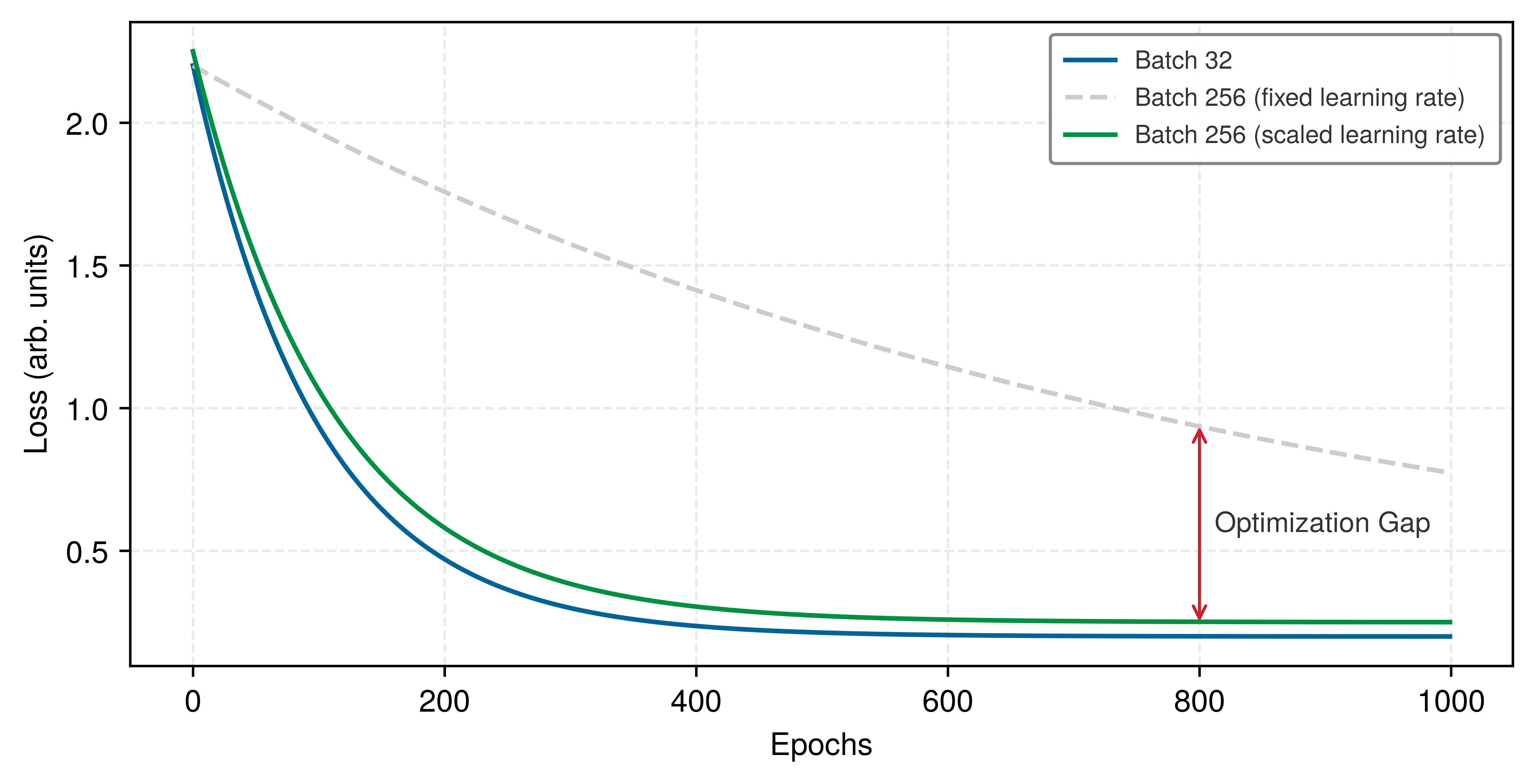
For a fixed dataset, doubling the global batch size halves the number of updates per epoch. The linear scaling rule (\(\eta_{\text{new}} = k \times \eta_{\text{base}}\)) is a useful empirical recipe over some batch-size ranges, often combined with learning-rate warmup, but it does not guarantee equivalent convergence or generalization. Figure 7 uses normalized synthetic curves to illustrate the intended effect.
Beyond the convergence effects, batch size interacts with distributed training strategies. A larger global batch reduces the number of optimizer steps and gradient synchronizations per epoch, while the payload of each dense synchronization is primarily determined by the parameter-gradient size rather than the batch size. In distributed settings, local and global batch sizes constrain the degree of data parallelism and the frequency of parameter updates. Gradient accumulation (section 1.5.5) decouples the effective batch size from the number of samples held for one micro-batch, though it does not remove the need to tune the effective batch size.
Napkin Math 1.5: The utility bill
Problem: Under the following simplified assumptions, is it cheaper to rent or purchase a 1,024-H100 cluster for one Llama 2 70-billion-parameter training run?
Math:
- Workload: Llama 2 70B model (70B parameters, 2T tokens).
- Compute required: \(6 \times 70 \times 10^9 \times 2 \times 10^{12} \approx 8.4 \times 10^{23}\) FLOPs. The leading factor of 6 follows from the chapter’s accounting: about 2 FLOPs per parameter per token in the forward pass (two FLOPs per multiply-accumulate), tripled once the backward pass, which costs roughly twice the forward pass, is included.
- Hardware: NVIDIA H100 (Peak: 989 TFLOP/s FP16). Assumed Utilization: 50 percent (494.5 TFLOP/s).
- Time: \(8.4 \times 10^{23} / (494.5 \times 10^{12}) \approx 1.70 \times 10^{9}\) seconds ≈ 53.8 years (on one GPU).
- Cluster: On 1,024 GPUs → 19.2 days.
The economics:
- Rental ($3/hr): 1,024 GPUs \(\times\) 24 hrs \(\times\) 19.2 days \(\times\) $3/hr ≈ $1.42M.
- Purchase ($30,000 per GPU): 1,024 GPUs \(\times\) $30,000 = $30.7M.
Systems insight: In this simplified utilization-and-price scenario, purchase cost equals about 21.7 rental runs. A real ownership comparison must also include cluster networking, host systems, facilities, power, staffing, depreciation, financing, and the utilization achieved between runs.
Every batch-size and precision decision so far has aimed at wall-clock time; at scale, that time is denominated in dollars. The compute cost itself becomes a binding constraint that shapes every training decision, from hardware selection to cluster sizing. The calculation here turns that cost into a rental-versus-purchase decision for a realistic training run.
This section established the structural what of training systems, and the mathematical foundations in section 1.2 quantified the FLOPs, memory, and bandwidth each stage demands. Yet understanding what must happen does not reveal where the system currently underperforms. A training pipeline is only as fast as its slowest stage: if data loading takes 50 ms and computation takes 100 ms, optimizing computation by 20 percent saves 20 ms, but if the bottleneck were data loading, those same engineering hours would save nothing. Before reaching for optimization techniques, diagnostic tools must identify which constraint actually limits performance.
Self-Check: Question
Which set of subsystems defines the chapter’s high-level training system architecture, and what systems engineering advantage does this decomposition provide?
- Storage controller, compiler intermediate representation, and runtime execution engine; this separates hardware target code generation from storage layout.
- Data pipeline, training loop, and evaluation pipeline; this separates distinct resource profiles (CPU/storage I/O, accelerator compute/memory, and periodic validation) so bottlenecks can be isolated at subsystem interfaces.
- Tokenizer, hyperparameter optimizer, and model registry; this organizes the model deployment lifecycle around developer interfaces.
- Gradient aggregator, parameter server, and checkpoint restorer; this decomposes cloud service microservices.
In a profiled training pipeline, CPU data preprocessing delivers batches at \(4\text{ GB/s}\), host-to-device PCIe transfer operates at \(32\text{ GB/s}\), and GPU compute consumes data at an equivalent rate of \(12\text{ GB/s}\). According to the pipeline bottleneck model, what determines end-to-end throughput, and what is the optimal first engineering action?
- The average rate of the three stages (\((4+32+12)/3 = 16\text{ GB/s}\)); apply incremental tuning across all stages simultaneously.
- The PCIe transfer rate (\(32\text{ GB/s}\)), because every batch must physically cross the bus; upgrade from PCIe Gen4 to Gen5.
- The minimum rate (\(4\text{ GB/s}\) at preprocessing); parallelize CPU preprocessing (e.g., via multi-worker DataLoader and prefetching) because the slowest stage caps total system throughput.
- The GPU compute rate (\(12\text{ GB/s}\)), because accelerator computation is always the primary cost driver in deep learning.
Explain why CPU-side tokenization and data augmentation can severely bottleneck GPU training even when the resulting tensor transfer across PCIe takes less than one millisecond.
Scaling the training batch size by \(8\times\) (e.g., from 512 to 4,096) while keeping the learning rate and schedule constant guarantees identical validation convergence in \(8\times\) less wall-clock time.
To enable fast, asynchronous Direct Memory Access (DMA) transfers from host RAM to GPU memory without intermediate CPU staging copies, host memory buffers must be allocated as page-locked or ____ memory.
Identifying Bottlenecks
Blueprint knowledge is not diagnosis. Knowing that attention operations consume 50 percent of FLOPs and data loading takes 25 percent of wall-clock time does not reveal which constraint to attack first; that depends on which resource is actually saturated during execution.
The diagnostic methodology that transforms blueprint knowledge into actionable optimization decisions begins with a meaningful measure of training efficiency. Raw accelerator utilization percentages can be misleading because an accelerator may remain active while executing recomputation, padding, or other work outside the model-FLOP accounting. Model FLOPs utilization (MFU)20 supplies that comparison.
20 Model FLOPs utilization (MFU): The PaLM paper (Chowdhery et al. 2022) defined MFU as observed throughput divided by the theoretical maximum throughput at peak FLOPs. Its 540-billion-parameter run reported 46.2 percent MFU on 6,144 TPU v4 chips. The complement is uncredited by the model-FLOP numerator, but MFU alone does not identify how much came from memory traffic, communication, pipeline bubbles, recomputation, or other work.
Chowdhery, Aakanksha, Sharan Narang, Jacob Devlin, Maarten Bosma, Gaurav Mishra, Adam Roberts, Paul Barham, et al. 2022. “PaLM: Scaling Language Modeling with Pathways.” arXiv Preprint arXiv:2204.02311.
Definition 1.4: Model FLOPs utilization (MFU)
Model FLOPs utilization (MFU) is the efficiency metric \(\text{MFU} = O_{\text{model}} / (R_{\text{peak}} \cdot T_{\text{step}})\), where \(O_{\text{model}}\) is the useful per-step model FLOP count (forward plus backward, excluding rematerialization) and \(T_{\text{step}}\) is the measured wall-clock time per training step, expressing what fraction of peak hardware throughput is doing useful model computation.
- Significance: MFU makes the effective-throughput term in the iron law concrete. For a 7B-parameter transformer processing 1,024 tokens per step on an A100 (312 TFLOP/s FP16/BF16 Tensor Core peak), a 1.2-second step gives model FLOPs divided by the available peak-rate FLOP budget of approximately 0.11 (11.5 percent). The remaining 88.5 percent is not credited as model FLOPs and can reflect memory traffic, communication, bubbles, non-model operations, or idle time. Whether a value is good depends on the model, hardware, precision, and parallelization strategy; diagnosis requires a profile rather than a universal threshold.
- Distinction: Hardware utilization reports whether device engines are active, whereas MFU credits the analytical model-FLOP estimate used in its numerator. It can therefore exclude recomputation and padding even when those operations keep the device busy. Comparisons across accelerators remain sensitive to the selected peak-throughput specification and FLOP-counting convention.
- Common pitfall: A frequent misconception is that 100 percent MFU is a realistic sustained target. Memory traffic, communication, and non-matrix work keep end-to-end runs below peak, but no universal 55–65 percent ceiling exists. Reported values depend on the model, precision, batch shape, hardware, and MFU definition, and can improve with FlashAttention and careful tuning.
Training bottlenecks can be investigated through three categories aligned with the D·A·M taxonomy (Data, Algorithm, Machine; The D·A·M Taxonomy provides the full diagnostic framework, troubleshooting matrix, and D·A·M Scorecard). Table 7 connects each axis to a common training bottleneck, its observable symptoms, and relevant optimization techniques. These are diagnostic starting points, not exclusive mappings.
| D·A·M Axis | Bottleneck | Symptoms | Primary Solutions |
|---|---|---|---|
| Algorithm | Compute-bound | High arithmetic-unit activity; additional bandwidth does not improve throughput; arithmetic throughput is limiting | Reduced precision, more efficient algorithms, faster compute hardware |
| Machine | Memory-bound | High memory-bandwidth use relative to arithmetic throughput; kernels stall on data movement | Operator fusion, memory-efficient attention, reduced precision formats |
| Data | Data-bound | Periodic accelerator utilization drops to near-zero; CPU fully busy during gaps; pipeline cannot feed GPU fast enough | Prefetching, pipeline overlap, faster storage, DataLoader parallelism |
The data-bound category is a commonly misdiagnosed bottleneck in practice.
Example 1.2: The GIL-locked GPU
Scenario: An engineering team builds a PyTorch data-loading pipeline using standard Python
threading for CPU-bound image preprocessing that holds the global interpreter lock (GIL).
Diagnosis: The GIL serializes these Python-level preprocessing threads, making host preparation time (\(T_{\text{prep}} \approx 250 \text{ ms}\)) vastly exceed GPU execution time (\(T_{\text{step}} \approx 12 \text{ ms}\)), collapsing hardware utilization to \(\eta_{\text{hw}} \approx 4.6\%\).
Systems lesson: Python CPU work that holds the GIL can serialize threads and starve GPUs; native operations may release it. Process workers (num_workers > 0) avoid interpreter serialization, while NVIDIA DALI can move eligible work off the host.
Profiling tools reveal which bottleneck dominates a given workload. Figure 8 captures the data-bound pathology from the callout: white gaps between repeated compute blocks mark intervals with no GPU kernels visible in the device timeline.
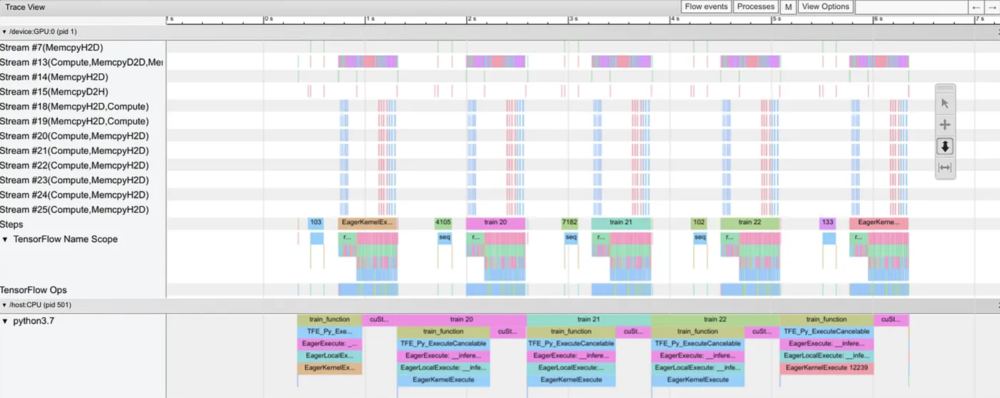
Four tools integrated into machine learning frameworks provide detailed bottleneck analysis. Table 8 separates framework-level timeline tools from GPU-level execution tools, because each exposes a different failure signature.
| Tool | Scope | Best signal |
|---|---|---|
PyTorch Profiler (torch.profiler) |
Framework-level operation trace | Time spent in each operation, memory allocation patterns, and GPU kernel execution |
| TensorFlow Profiler | Framework-level training timeline | Input pipeline bottlenecks and device placement |
| NVIDIA Nsight Systems | System-level GPU trace | Kernel execution, memory transfers, and synchronization points |
| NVIDIA Nsight Compute | Kernel-level GPU analysis | Arithmetic intensity, memory throughput, and occupancy |
The profiling workflow follows a systematic pattern: run a representative training iteration with profiling enabled, examine the timeline for gaps (data-bound), check memory bandwidth utilization (memory-bound vs. compute bound), and identify the dominant bottleneck before selecting an optimization technique.
In practice, the characteristic signatures from table 7 are directly visible in profiler traces: accelerator utilization levels, memory bandwidth saturation, and CPU vs. GPU activity ratios each point to a specific bottleneck class. These signatures map to specific optimization techniques: prefetching for data bottlenecks, mixed precision and operator fusion for memory bottlenecks, and algorithmic improvements or hardware upgrades for compute bottlenecks. With a diagnostic framework in hand, the next step is to examine each optimization technique in detail: what it does, which iron law term it targets, and when profiling results indicate it should be applied.
Self-Check: Question
Why is Model FLOPs Utilization (MFU) a more reliable metric than raw GPU busy percentage (reported by tools like
nvidia-smi) when evaluating training systems efficiency?- MFU is measured directly from host CPU clock cycles, eliminating GPU driver instrumentation overhead.
- MFU is mathematically fixed to 100% on any healthy accelerator cluster regardless of software overhead.
- MFU counts only the theoretical forward and backward FLOPs required by the model architecture divided by peak hardware throughput, whereas raw GPU busy percentage also credits uncredited recomputation, padding tokens, and memory stalls that do not advance model training.
- MFU measures training loss convergence speed per dollar rather than floating-point operations.
An engineer profiles two training workloads. Workload A exhibits 92 percent GPU utilization, near-saturated HBM bandwidth, low CPU activity, and continuous kernel timelines. Workload B exhibits 20 percent GPU utilization with regular 50 ms idle gaps on the GPU timeline, low HBM bandwidth, and 100 percent CPU utilization. Apply the D·A·M taxonomy to classify each workload’s bottleneck and state the primary optimization category for each.
Order the steps of the systematic training optimization workflow recommended in the chapter:
- Classify the primary performance constraint (Data-, Memory-, or Compute-bound) using the D·A·M taxonomy.
- Run a representative training run with framework and system profilers enabled to capture CPU, PCIe, and GPU timeline traces.
- Re-profile the system to evaluate MFU improvement and identify whether the bottleneck has shifted to a new pipeline stage.
- Apply a targeted optimization technique specifically addressing the identified binding constraint.
An engineering team suspects that an individual custom LayerNorm kernel has poor arithmetic intensity and low register occupancy, while another team suspects their DataLoader is causing host-to-device PCIe transfer stalls. Which combination of profiling tools from the chapter is best suited to investigate each respective issue?
- NVIDIA Nsight Compute for the kernel-level arithmetic intensity and occupancy analysis; NVIDIA Nsight Systems (or PyTorch Profiler) for system-level timeline visualization of DataLoader and PCIe transfers.
nvidia-smifor kernel-level arithmetic intensity; TensorBoard loss curves for DataLoader PCIe transfer stalls.- NVIDIA Nsight Compute for cluster-wide inter-node network bandwidth; PyTorch Profiler for register allocation analysis.
- Linux
topcommand for GPU kernel instruction analysis; NVIDIA Nsight Systems for CPU register spill tracking.
Pipeline Optimizations
Profiling reveals where the training system underperforms; the D·A·M taxonomy (The D·A·M Taxonomy) classifies what kind of bottleneck limits throughput. The remaining question is how to close the gap. Four optimization techniques, each targeting a specific bottleneck category, together with a systematic framework for composing them, provide the answer.
Even well-designed pipeline architectures rarely reach hardware peak throughput without targeted optimization. To illustrate the scale of the gap, applying a model-FLOP utilization of 30 percent to 50 percent to an A100 peak of 312 TFLOP/s gives 93.6 TFLOP/s–156 TFLOP/s of model-FLOP throughput. These are derived scenario values, not measurements reported for one A100 workload. Published large-model systems report similar gaps between peak and realized throughput (Narayanan et al. 2021; Chowdhery et al. 2022). Systems such as SuperNeurons show one version of this problem: memory-management bottlenecks can prevent larger networks from training efficiently unless the runtime actively optimizes activation storage and transfer (Wang et al. 2018). Table 9 extends the D·A·M-based bottleneck classification from table 7 by mapping each bottleneck to the specific optimization technique that addresses it.
Narayanan, Deepak, Mohammad Shoeybi, Jared Casper, Patrick LeGresley, Mostofa Patwary, Vijay Korthikanti, Dmitri Vainbrand, et al. 2021. “Efficient Large-Scale Language Model Training on GPU Clusters Using Megatron-LM.” Proceedings of the International Conference for High Performance Computing, Networking, Storage and Analysis, 1–15. https://doi.org/10.1145/3458817.3476209.
Wang, Linnan, Jinmian Ye, Yiyang Zhao, Wei Wu, Ang Li, Shuaiwen Leon Song, Zenglin Xu, and Tim Kraska. 2018. “SuperNeurons: Dynamic GPU Memory Management for Training Deep Neural Networks.” Proceedings of the 23rd ACM SIGPLAN Symposium on Principles and Practice of Parallel Programming, 41–53. https://doi.org/10.1145/3178487.3178491.
| Bottleneck | Primary Solution(s) |
|---|---|
| Data Movement Latency | Prefetching & Pipeline Overlapping |
| Compute Throughput | Mixed-Precision Training |
| Memory Capacity | Gradient Accumulation & Activation Checkpointing |
| Memory Bandwidth (Attn.) | FlashAttention (IO-aware tiling) |
These bottlenecks manifest differently across system scales (a 100 GB model faces different constraints than a 1 GB model), but identification and mitigation follow consistent principles. Data movement latency emerges when training batches cannot flow from storage through preprocessing to compute units fast enough to keep accelerators in use. Computational throughput limitations occur when mathematical operations execute below hardware peak performance due to suboptimal precision choices or kernel inefficiencies. Memory capacity constraints restrict both the model sizes and batch sizes a system can process, directly limiting model complexity and training efficiency.
These bottlenecks interact, illustrating the conservation of complexity thesis from Part I: relieving one constraint can expose another. When data loading becomes a bottleneck, GPUs sit idle waiting for batches. When memory capacity is constrained, smaller batches may reduce GPU efficiency. For a hypothetical GPT-2 profile, suppose attention occupies 50 percent of time, data loading 25 percent, and other compute-bound operations 25 percent. Such a profile motivates evaluating memory-efficient attention, prefetching, and reduced precision, then measuring again to see which change matters. The optimization challenge is to identify the current bottleneck and select techniques that address it without creating a worse constraint elsewhere.
Systematic optimization framework
The profile example shows why optimization must start from evidence rather than preference. Effective optimization follows a systematic methodology that applies regardless of system scale or model architecture: profile to identify bottlenecks, select appropriate techniques for the identified constraints, and compose solutions that address multiple bottlenecks simultaneously without creating conflicts.
The profiling phase employs tools like PyTorch Profiler, TensorFlow Profiler, or NVIDIA Nsight Systems to reveal where time is spent during training iterations. These are the same profiling approaches introduced in the overview, now applied systematically to quantify which bottleneck dominates. A profile might show 40 percent of time in data loading, 35 percent in computation, and 25 percent in memory operations, indicating data loading as the primary target for optimization.
The selection phase matches optimization techniques to identified bottlenecks. Each technique targets specific constraints. Prefetching addresses data movement latency, mixed-precision training tackles both computational throughput and memory constraints, and gradient accumulation manages memory limitations. Selection requires understanding the bottleneck type alongside the characteristics of the hardware, model architecture, and training configuration that influence technique effectiveness.
The composition phase combines multiple techniques to achieve cumulative benefits. Prefetching and mixed-precision training complement each other (one addresses data loading, the other computation and memory), allowing simultaneous application. However, some combinations create conflicts: aggressive prefetching increases memory pressure, potentially conflicting with memory-constrained configurations. Successful composition requires understanding technique interactions and dependencies.
This systematic framework (profile, select, compose) applies to the four core optimization techniques covered next. Prefetching targets data movement latency. Mixed-precision training addresses both throughput and memory constraints. FlashAttention reduces memory traffic for attention. Gradient accumulation manages batch-memory limits by serializing micro-batches, while checkpointing trades recomputation for lower activation storage. The profile should determine the order in which these techniques are evaluated, and each requires a cost-benefit analysis that includes implementation and debugging effort.
Figure 9 provides a decision tree that operationalizes this systematic framework. The branches lead from profiling results through bottleneck identification to technique selection, ensuring optimization effort targets the actual constraint rather than perceived issues.
\begin{tikzpicture}[font=\small\sffamily, line width=0.8pt]
% Color palette aligned with chapter diagrams
\definecolor{BlueLine}{HTML}{006395}
\definecolor{BlueL}{HTML}{D1E6F3}
\definecolor{GreenLine}{HTML}{008F45}
\definecolor{GreenL}{HTML}{D4EFDF}
\definecolor{RedLine}{HTML}{CC0000}
\definecolor{RedL}{HTML}{F5D6D6}
\definecolor{VioletLine}{HTML}{702082}
\definecolor{VioletL}{HTML}{D8C2DE}

\tikzset{
  Flow/.style={->, >=latex, draw=black!65, line width=0.85pt},
  StartStop/.style={
    draw=VioletLine, fill=VioletL2, rounded corners=12pt,
    minimum width=3.9cm, minimum height=0.9cm, align=center, font=\small\sffamily
  },
  Decision/.style={
    draw=BlueLine, fill=cyan!10, diamond, aspect=2.2,inner sep= -1ex,
    minimum width=4.3cm, minimum height=2cm, align=center, font=\small\sffamily
  },
  Bottleneck/.style={
    draw=GreenLine, fill=GreenL!50,
    minimum width=3.5cm, minimum height=1.1cm, align=center, font=\small\sffamily
  },
  Action/.style={
    draw=RedLine, fill=magenta!10,
    minimum width=3.5cm, minimum height=1.1cm, align=center, font=\small\sffamily
  },
  BranchLabel/.style={font=\scriptsize\sffamily, fill=white, inner sep=1.2pt}
}

% Nodes
\node[StartStop] (profile) at (0,0) {Profile Training Run};
\node[Decision,below =0.6 of profile] (util) {Accelerator\\ Util $<70\%$?};
% Data Branch (Left)
\node[Bottleneck, left=2.5 of util] (data) {Data-Bound};
\node[Action,below = 0.7 of data ] (prefetch)  {Apply Prefetching \&\\Pipeline Overlap};

% Memory Check (Center)
\node[Decision,below=1.6 of util] (memq)  {OOM Errors or\\Mem $>90\%$?};

% Memory Branch (Left-Center)
\node[Bottleneck,left =2.50 of memq] (memb)  {Memory-Bound};
\node[Action,below =0.7 of memb] (memact)  {Mixed Precision, \\Checkpointing,\\Accumulation};
% Compute Branch (Right)
\node[Bottleneck,right= 2.50 of memq] (compb) {Compute-Bound};
\node[Action,below =0.7 of compb] (compact) {Increase Batch Size,\\Optimize Kernels};
% End Node
\node[StartStop,below =2.0 of memq] (reprofile) {Re-profile \& Iterate};
% Main flow connections
\draw[Flow] (profile.south) -- (util.north);
\draw[Flow] (util) --node[above=1pt,pos=0.2, BranchLabel] {Yes}(data) ;
\draw[Flow] (util.south) -- (memq.north) node[pos=0.1, right=1pt,BranchLabel] {No};
\draw[Flow] (data.south) -- (prefetch.north);
\draw[Flow] (memq) -- node[above=1pt,pos=0.2, BranchLabel] {Yes}(memb);
\draw[Flow] (memq.east) --node[above=1pt,pos=0.2, BranchLabel] {No} (compb);
\draw[Flow] (memb.south) -- (memact.north);
\draw[Flow] (compb.south) -- (compact.north);
\draw[Flow] (memact.south)--++(0,-0.5)|-(reprofile);
\draw[Flow] (compact.south)--++(0,-0.5)|-(reprofile);
%
\draw[Flow] (prefetch.west)--++(-0.5,0)|-(reprofile);
\end{tikzpicture}The flowchart embodies a critical insight: optimization is iterative. After applying a technique, re-profiling often reveals that a different bottleneck has become dominant. A data-bound system that implements prefetching may become memory bound, requiring the next technique in the decision tree. This iterative refinement continues until profiling shows balanced resource utilization or acceptable training throughput.
Data prefetching and overlapping
Prefetching and overlapping techniques illustrate the systematic framework in action, targeting data movement latency bottlenecks by coordinating data transfer with computation. This optimization proves most effective when profiling reveals that computational units remain idle while waiting for data transfers to complete.
Training machine learning models involves significant data movement between storage, memory, and computational units. The data pipeline consists of sequential transfers: from disk storage to CPU memory, CPU memory to GPU memory, and through the GPU processing units. In ML training, a “Read” operation is rarely a simple disk fetch: for image workloads it encompasses JPEG decoding, random crops, and color jitter applied on CPU cores before the tensor is ready to transfer; for language workloads it encompasses tokenization, subword encoding, and sequence padding. Figure 10 exposes the inefficiency of sequential data transfer: the GPU remains idle during file operations (Open 1, Open 2), and training steps cannot begin until these read and preprocessing operations complete, leaving expensive compute resources underutilized for significant portions of each epoch.
Prefetching addresses these inefficiencies by loading data into memory before its scheduled computation time. During the processing of the current batch, framework data pipelines such as tf.data load and prepare subsequent batches, maintaining a consistent supply of ready data (Murray et al. 2021).
Murray, Derek G., Jiřı́ Šimša, Ana Klimovic, and Ihor Indyk. 2021. “Tf.data: A Machine Learning Data Processing Framework.” Proceedings of the VLDB Endowment 14 (12): 2945–58. https://doi.org/10.14778/3476311.3476374.
\begin{tikzpicture}[
  font=\small\sffamily,
  line width=0.75pt,
  execute at begin picture={
    %
    \def\W{128mm}   % total width of the diagram (time axis)
    \def\Tmax{95}   % total duration (units on x-axis)
    \def\rowH{9mm}  % row height
    %
    \pgfmathsetlengthmacro{\Xunit}{\W/\Tmax}
    \tikzset{x=\Xunit, y=\rowH}
  }
]
\tikzset{%
  box/.style={rounded corners=0pt, draw, line width=.5pt},
  open/.style ={box, fill=cOpen,  draw=gray!80},
  read/.style ={box, fill=cRead,  draw=BlueLine},
  train/.style={box, fill=cTrain, draw=GreenLine},
  epoch/.style={box, fill=cEpoch, draw=OrangeLine},
  tick/.style={draw=gray!50, line width=.25pt},
  gridline/.style={draw=gray!25, line width=.2pt},
}
% ---------------------------
% SETTINGS
% ---------------------------
% Standard color definitions
\definecolor{BlueLine}{HTML}{006395}
\definecolor{BlueL}{HTML}{D1E6F3}
\definecolor{GreenLine}{HTML}{008F45}
\definecolor{GreenL}{HTML}{D4EFDF}
\definecolor{OrangeLine}{HTML}{CC5500}
\definecolor{OrangeL}{HTML}{FFE5CC}
% Colors
\colorlet{cOpen}{gray!20}
\colorlet{cRead}{cyan!15}
\colorlet{cTrain}{GreenL!80}
\colorlet{cEpoch}{orange!10}
% ---------------------------
% COORDINATES OF ROWS (from top to bottom)
% ---------------------------
% y = 3: Open, 2: Read, 1: Train, 0: Epoch
\def\yOpen{3}
\def\yRead{2}
\def\yTrain{1}
\def\yEpoch{0}

% ---------------------------
%  BACKGROUND GRID (vertical lines)
% ---------------------------
% Every 5 min a thin line, every 15 min a little darker
\foreach \t in {0,5,...,\Tmax} {
  \draw[gridline] (\t, -0.4) -- (\t, 4.2);
}
\foreach \t in {0,15,...,\Tmax} {
  \draw[tick] (\t, -0.4) -- (\t, 4.2);
}

% ---------------------------
%LEFT LINE MARKS
% ---------------------------
\node[anchor=east] at (0,\yOpen+0.5)  {$\,$Open};
\node[anchor=east] at (0,\yRead+0.5)  {$\,$Read};
\node[anchor=east] at (0,\yTrain+0.5) {$\,$Train};
\node[anchor=east] at (0,\yEpoch+0.5) {$\,$Epoch};

% ---------------------------
% LEVE OZNAKE REDOVA
% ---------------------------
% \bar{stil}{y}{start}{end}{tekst}
\renewcommand{\Bar}[5]{%
  \path (#3, #2+0.18) coordinate (A);
  \path (#4, #2+0.82) coordinate (B);
  \draw[#1] (A) rectangle (B);
  \node[font=\scriptsize\sffamily, anchor=center] at ($ (A)!0.5!(B) $) {#5};
}
% ---------------------------
% BARS
% ---------------------------
% Open
\Bar{open}{\yOpen}{0}{7.5}{Open 1}
\Bar{open}{\yOpen}{60}{67.5}{Open 2}
% Read
\Bar{read}{\yRead}{7.5}{20}{Read 1}
\Bar{read}{\yRead}{20}{30}{Read 2}
\Bar{read}{\yRead}{67.5}{80}{Read 3}
% Train
\Bar{train}{\yTrain}{30}{45}{Train 1}
\Bar{train}{\yTrain}{45}{60}{Train 2}
\Bar{train}{\yTrain}{80}{95}{Train 3}
% Epoch
\Bar{epoch}{\yEpoch}{0}{60}{Epoch 1}
\Bar{epoch}{\yEpoch}{60}{95}{Epoch 2}

% ---------------------------
% LOWER TIME AXIS (labels on 15 min)
% ---------------------------
\def\yAxis{-0.55}

\foreach \t/\lbl in {
  0/00:00,
  15/00:15,
  30/00:30,
  45/00:45,
  60/01:00,
  75/01:15,
  90/01:30,
  95/01:35
}{
  \node[font=\scriptsize\sffamily, anchor=north] at (\t,\yAxis+0.20) {\lbl};
}
\end{tikzpicture}Overlapping extends prefetching by coordinating multiple pipeline stages to execute concurrently. The system processes the current batch while simultaneously preparing future batches through data loading and preprocessing operations. Compare the illustrative schedules in figure 10 and figure 11. Under their assumed stage durations, overlap reduces completion time from approximately 95 min to 65 min, a 31.6 percent reduction. Actual gains depend on stage balance and available concurrency.
\begin{tikzpicture}[
  font=\small\sffamily,
  line width=0.75pt,
  execute at begin picture={
    %
    \def\W{140mm}   % total width of the diagram (time axis)
    \def\Tmax{65}   % total duration (units on x-axis)
    \def\rowH{9mm}  % row height
    %
    \pgfmathsetlengthmacro{\Xunit}{\W/\Tmax}
    \tikzset{x=\Xunit, y=\rowH}
  }
]
\tikzset{%
  box/.style={rounded corners=0pt, draw, line width=.5pt},
  open/.style ={box, fill=cOpen,  draw=gray!80},
  read/.style ={box, fill=cRead,  draw=BlueLine},
  train/.style={box, fill=cTrain, draw=GreenLine},
  epoch/.style={box, fill=cEpoch, draw=OrangeLine},
  tick/.style={draw=gray!50, line width=.25pt},
  gridline/.style={draw=gray!25, line width=.2pt},
}
% ---------------------------
% SETTINGS
% ---------------------------
% Standard color definitions
\definecolor{BlueLine}{HTML}{006395}
\definecolor{BlueL}{HTML}{D1E6F3}
\definecolor{GreenLine}{HTML}{008F45}
\definecolor{GreenL}{HTML}{D4EFDF}
\definecolor{OrangeLine}{HTML}{CC5500}
\definecolor{OrangeL}{HTML}{FFE5CC}
% Colors
\colorlet{cOpen}{gray!20}
\colorlet{cRead}{cyan!15}
\colorlet{cTrain}{GreenL!80}
\colorlet{cEpoch}{orange!10}
% ---------------------------
% COORDINATES OF ROWS (from top to bottom)
% ---------------------------
% y = 3: Open, 2: Read, 1: Train, 0: Epoch
\def\yOpen{3}
\def\yRead{2}
\def\yTrain{1}
\def\yEpoch{0}

% ---------------------------
%  BACKGROUND GRID (vertical lines)
% ---------------------------
% Every 5 min a thin line, every 15 min a little darker
\foreach \t in {0,5,...,\Tmax} {
  \draw[gridline] (\t, -0.4) -- (\t, 4.2);
}
\foreach \t in {0,15,...,\Tmax} {
  \draw[tick] (\t, -0.4) -- (\t, 4.2);
}
% ---------------------------
%LEFT LINE MARKS
% ---------------------------
\node[anchor=east] at (0,\yOpen+0.5)  {$\,$Open};
\node[anchor=east] at (0,\yRead+0.5)  {$\,$Read};
\node[anchor=east] at (0,\yTrain+0.5) {$\,$Train};
\node[anchor=east] at (0,\yEpoch+0.5) {$\,$Epoch};

% ---------------------------
% LEVE OZNAKE REDOVA
% ---------------------------
% \bar{stil}{y}{start}{end}{tekst}
\renewcommand{\Bar}[5]{%
  \path (#3, #2+0.18) coordinate (A);
  \path (#4, #2+0.82) coordinate (B);
  \draw[#1] (A) rectangle (B);
  \node[font=\scriptsize\sffamily, anchor=center] at ($ (A)!0.5!(B) $) {#5};
}
% ---------------------------
% BARS
% ---------------------------
% Open
\Bar{open}{\yOpen}{0}{7.5}{Open 1}
\Bar{open}{\yOpen}{30}{37.5}{Open 2}
% Read
\Bar{read}{\yRead}{7.5}{20}{Read 1}
\Bar{read}{\yRead}{20}{30}{Read 2}
\Bar{read}{\yRead}{37.5}{50}{Read 3}
% Train
\Bar{train}{\yTrain}{20}{35}{Train 1}
\Bar{train}{\yTrain}{35}{50}{Train 2}
\Bar{train}{\yTrain}{50}{65}{Train 3}

% Epoch
\Bar{epoch}{\yEpoch}{0}{65}{Epochs (Overlapped)}
% ---------------------------
% LOWER TIME AXIS (labels on 15 min)
% ---------------------------
\def\yAxis{-0.55}

\foreach \t/\lbl in {
  0/00:00,
  15/00:15,
  30/00:30,
  45/00:45,
  60/01:00,
  65/01:05
}{
  \node[font=\scriptsize\sffamily, anchor=north] at (\t,\yAxis+0.20) {\lbl};
}
\end{tikzpicture}Prefetching mechanics
Prefetching only pays off when the profile shows data movement on the critical path. Training data still passes through retrieval, transformation, and model execution; the optimization changes when those stages run. An unoptimized pipeline serializes them, leaving the GPU idle during data fetching and preprocessing. Data loaders avoid that stall by preparing the next batch in separate threads or processes while the current batch trains.
Overlapping extends the same idea across the full pipeline. As the GPU processes one batch, preprocessing begins on the next batch, while data fetching starts for the subsequent batch. The goal is constant activity at each stage so the slowest stage no longer leaves the others waiting.
Machine learning frameworks (introduced in ML Frameworks) expose the control variables for this trade-off. Listing 4 demonstrates PyTorch’s DataLoader configuration, where num_workers = 4 sets preprocessing parallelism and prefetch_factor = 2 maintains a buffer of 8 batches ready for accelerator consumption.
loader = DataLoader(
    dataset, batch_size=32, num_workers=4, prefetch_factor=2
)
The parameters num_workers and prefetch_factor are not generic performance toggles. They determine CPU parallelism and buffer depth, which means they shift pressure from accelerator idle time to host memory and CPU scheduling.
Buffer management is the main trade-off. A buffer that is too small causes the GPU to wait for data preparation, reintroducing the idle time prefetching was meant to remove. An overly large buffer consumes memory that could otherwise store model parameters or larger batches. The right configuration coordinates CPU preparation, storage I/O, and GPU computation so each resource has work ready at the moment it can use it. These techniques yield the greatest benefit when storage access is slow, preprocessing is complex, or datasets are large.
Practical considerations
Prefetch buffers and overlap depth are tunable, so the same machinery adapts to whichever stage binds, whether slow storage, limited network bandwidth, or computational throughput. Prefetching and overlapping deliver the greatest gains when preprocessing lies on the critical path but can run concurrently with model computation. In an illustrative image pipeline, random cropping (10 ms), color jittering (15 ms), and normalization (5 ms) total 30 ms per batch. Overlap can hide up to the concurrent accelerator-computation time; any excess remains on the critical path. NLP workloads similarly benefit when tokenization and subword processing would otherwise block the training loop.
The primary trade-off is memory: prefetch buffers consume host memory, or device memory when a separate device-side queue is used, in proportion to buffer depth and batch size. With batch size 256 high-resolution images (\(1024\times 1024\) pixels), one buffered batch requires approximately 3.2 GB. With num_workers = 4 and prefetch_factor = 2, the 8-batch prefetch window can hold about 25.8 GB. Tuning these parameters requires empirical testing because excessive workers contend for CPU, storage, and memory resources, while insufficient buffering reintroduces data stalls. Start with a modest worker count, increase it while measuring throughput and memory, and stop when additional workers no longer reduce accelerator idle time. When the input pipeline already exceeds compute demand, deeper prefetching adds complexity without improving throughput.
Mixed-precision training
While prefetching optimizes data movement, mixed-precision training addresses both computational throughput limitations and memory capacity constraints. It uses a lower-precision format where appropriate while retaining higher precision for selected accumulations or updates. Numerical Representations compares FP32, FP16, BF16, FP8, and INT8 precision-range trade-offs. A training recipe commonly combines FP32 with either FP16 or BF16; it does not ordinarily use FP16 and BF16 interchangeably in the same path. The resulting speed, memory, and accuracy effects depend on the workload and hardware (Micikevicius et al. 2017; Wang and Kanwar 2019; Kalamkar et al. 2019).
A neural network’s stored FP32 weights require 4 bytes per parameter, while FP16 and BF16 weights use 2 bytes. For a model with \(10^9\) parameters, the weight tensor shrinks from 4 GB to 2 GB. Total training memory falls by less when the recipe retains FP32 master weights, optimizer states, or selected activations.
The numerical differences between these formats shape their use cases. Table 10 shows that BF16’s 8-bit exponent gives it approximately the same normal exponent range as FP32, while FP16’s 5-bit exponent gives a minimum positive normal value of about \(6.1 \times 10^{-5}\) and a maximum finite value of \(65{,}504\). FP16 subnormals extend toward \(6 \times 10^{-8}\), although their treatment depends on the operation and hardware mode. FP32 provides about seven decimal digits of precision, FP16 about three, and BF16 about two to three. BF16 therefore trades mantissa precision for the exponent range that often simplifies deep-learning training.
| Property | FP32 | FP16 | BF16 |
|---|---|---|---|
| Exponent bits | 8 | 5 | 8 |
| Mantissa bits | 23 | 10 | 7 |
| Min normal value | \(10^{-38}\) | \(6.1 \times 10^{-5}\) | \(10^{-38}\) |
| A100 peak throughput ratio | 1\(\times\) | 16× | 16× |
The choice between formats depends on model characteristics and hardware support. BF16’s wider exponent range can reduce overflow and underflow concerns, while FP16 provides more mantissa bits but often requires loss scaling. Framework autocast policies and fused kernels choose higher-precision accumulation for numerically sensitive operations when needed; loss reduction, softmax, normalization, and optimizer updates are common candidates, but their exact execution dtype is implementation-dependent.
Figure 12 traces a conventional FP16 mixed-precision recipe. FP32 master weights are cast for lower-precision computation, the loss is scaled before backpropagation, and gradients are unscaled before the FP32 update. Modern framework implementations may store or accumulate particular tensors differently, and BF16 recipes commonly omit loss scaling because of their wider exponent range.
\begin{tikzpicture}[font=\footnotesize\sffamily, line width=0.75pt, node distance=1.2cm]
% Standard color definitions
\definecolor{BlueLine}{HTML}{006395}
\definecolor{BlueL}{HTML}{D1E6F3}
\definecolor{GreenLine}{HTML}{008F45}
\definecolor{GreenL}{HTML}{D4EFDF}
\definecolor{RedLine}{HTML}{CB202D}
\definecolor{RedL}{HTML}{F5D2D5}
\definecolor{OrangeLine}{HTML}{CC5500}
\definecolor{OrangeL}{HTML}{FFE5CC}

\tikzset{
  Box/.style={
    rectangle, draw=black!50, line width=0.75pt,
    text width=25mm, align=center,
    minimum height=10mm
  },
  FP32Box/.style={
    Box, draw=BlueLine, fill=cyan!10
  },
  FP16Box/.style={
    Box, draw=GreenLine, fill=GreenL!60
  },
  ScaledBox/.style={
    Box, draw=RedLine, fill=magenta!10
  },
  Line/.style={
    draw=black!40, line width=1.0pt, ->,>=latex
  },
  StepLabel/.style={
    fill=white, inner sep=2pt, font=\scriptsize\bfseries\sffamily
  }
}

% Nodes
\node[FP32Box] (grad32) {FP32\\ Gradients};
\node[FP32Box, right=2.5 of grad32] (master) {FP32 Master\\ Weights};
\node[FP16Box, below=0.85 of master] (weights16) {FP16\\ Weights};
\node[FP16Box, below=0.85 of weights16] (forward) {Forward Pass\\ (FP16 Loss)};
\node[ScaledBox, left=2.5 of forward] (scaled) {Scaled Loss\\ (FP32)};
\node[ScaledBox, above=0.85 of scaled] (grad16) {Scaled FP16\\ Gradients};

% Cycle Connections
\draw[Line] (master) -- node[StepLabel,pos=0.42] {1. Cast} (weights16);
\draw[Line] (weights16) -- node[StepLabel,pos=0.42] {2. Forward} (forward);
\draw[Line] (forward) -- node[StepLabel] {3. Scale} (scaled);
\draw[Line] (scaled) -- node[StepLabel,pos=0.42] {4. Backprop} (grad16);
\draw[Line] (grad16) -- node[StepLabel,pos=0.42] {5. Copy \& Unscale} (grad32);
\draw[Line, dashed] (grad32) -- node[StepLabel] {6. Update} (master);

\end{tikzpicture}Modern hardware architectures are specifically designed to accelerate reduced precision computations. NVIDIA Tensor Cores were introduced for FP16 mixed-precision operations (NVIDIA 2017), and later A100-class Tensor Cores added BF16 support (NVIDIA Corporation 2020). Google’s TPUs natively support BF16, as this format was specifically designed for machine learning workloads (Wang and Kanwar 2019). These architectural optimizations typically enable substantially higher computational throughput for reduced precision operations compared to FP32, making mixed-precision training particularly efficient on modern hardware.
NVIDIA. 2017. Training with Mixed Precision.
NVIDIA Corporation. 2020. NVIDIA A100 Tensor Core GPU Architecture. NVIDIA Whitepaper, V1.0.
Mixed-precision training turns those hardware capabilities into a split numerical contract. Eligible matrix multiplications and convolutions use FP16 or BF16 inputs on Tensor Core paths, while selected reductions, accumulations, and parameter updates retain higher precision. The performance gain comes from both arithmetic and data movement. Lower-precision kernels can execute at higher throughput, and smaller activations or gradients reduce memory traffic when the recipe stores or communicates them in that format. Higher precision remains necessary where wide reductions, small parameter updates, or sensitive normalization can accumulate rounding error. The division is not universal. Frameworks choose dtypes per operation, kernels may accumulate in FP32, BF16 often avoids loss scaling, and optimizers may retain FP32 master weights and states. Mixed precision therefore coordinates formats across the training step instead of running every operation in one reduced precision.
Loss scaling
One of the key challenges with FP16 is its reduced dynamic range,21 which increases the likelihood of gradient values becoming too small to be represented accurately. Loss scaling addresses this issue by temporarily amplifying gradient values during backpropagation. Specifically, the loss value is scaled by a large factor (e.g., \(2^{10}\)) before gradients are computed, ensuring they remain within the representable range of FP16.
21 FP16 (half-precision floating-point): Its reduced normal range stems from using 5 exponent bits, compared with 8 in FP32; the smallest positive normal value is about \(6.1 \times 10^{-5}\), but subnormal values extend to about \(6 \times 10^{-8}\). Underflow behavior depends on the operation and hardware mode. Loss scaling reduces the chance that small gradients are rounded or flushed to zero.
Machine learning frameworks provide built-in support for mixed-precision training. PyTorch’s torch.amp (automatic mixed precision) library automates the process of selecting operation precision and can apply loss scaling when necessary.
Mixed-precision benefits
Mixed-precision benefits manifest across three dimensions that compound in practice:
- Weight memory: Decreases by 50 percent. A one-billion-parameter transformer’s weights require 4 GB in FP32 but 2 GB in FP16 or BF16. Total training-memory savings depend on retained higher-precision state.
- Computational throughput: Can increase when eligible operations use higher-throughput Tensor Core paths (section 1.5.3.3).
- Communication bandwidth: Can decrease when the distributed strategy communicates lower-precision tensors; some strategies still reduce or communicate gradients in FP32.
These benefits compound: a practitioner might simultaneously double batch size (memory savings), accelerate each iteration (Tensor Core throughput), and reduce gradient synchronization time (smaller tensors). On GPT-2, the combined effect is visible in both the memory budget and the training throughput.
Napkin Math 1.6: GPT-2 mixed precision memory savings
Problem: Can GPT-2 XL (1.5B parameters) be trained on a single V100 GPU, and what does mixed precision plus gradient checkpointing buy us in memory footprint?
FP32 baseline:
- Parameters and gradients (FP32): 12 GB (6 GB parameters + 6 GB gradients)
- Activations (batch = 4): ~71.7 GB
- Optimizer states (Adam m, v in FP32): 12 GB
- Total: ~95.7 GB (exceeds any single GPU)
FP16 mixed precision:
- Parameters (FP16): 1.5B parameters at 2 bytes each = 3 GB
- Activations (FP16): ~35.9 GB
- Gradients (FP16): 3 GB
- FP32 master weights: 6 GB (for precise optimizer updates)
- Optimizer states (Adam m, v in FP32): 12 GB
- Total: ~59.9 GB (still tight, but manageable with optimizations)
Mixed precision + illustrative fourfold activation reduction:
- Activations reduced to ~9 GB through selective recomputation
- Estimated tensor total: ~33 GB, compared with 32 GB of V100 capacity, before temporary workspaces and allocator overhead
Systems insight: Mixed precision halves the parameter and gradient tensors in this recipe; checkpointing then trades recomputation for lower activation storage. At batch size 4, the simplified tensor estimate approaches V100 capacity, so an actual run may still require additional memory reduction after accounting for workspaces and allocator behavior. At batch 32, the same estimate requires ~95.7 GB, motivating the scaling techniques later in this chapter.
Memory savings alone do not guarantee correct or stable training. FP16’s limited dynamic range demands specific implementation choices to keep gradients representable and weight updates nonzero.
Three implementation details support conventional FP16 mixed precision:
- Loss scaling: Multiplies the loss before backpropagation so that small gradients are less likely to underflow. Dynamic scalers adjust the factor in response to detected nonfinite gradients rather than relying on one universal starting value or range.
- FP32 master weights: In recipes that use them, preserve updates that could round away if applied directly to FP16 weights.
- Autocast policies: Select lower or higher precision per operation. Reductions, normalization, and softmax commonly use higher-precision accumulation, but the exact policy depends on the framework and kernel.
With these stability mechanisms in place, the gains from mixed precision are measurable in throughput and dollars.
Mixed precision is not automatic. FP16’s restricted exponent range can cause overflow or underflow, and subnormal handling varies by operation and hardware. Dynamic loss scaling addresses gradient-range failures, while monitoring for nonfinite losses, gradients, and activations remains essential. BF16 preserves FP32’s exponent range and usually avoids loss scaling, but its shorter mantissa still changes rounding behavior. For small or non-Tensor-Core-dominated workloads, conversion and scaling overhead can outweigh the performance benefit; profiling, rather than a parameter-count threshold, determines the result.
Napkin Math 1.7: GPT-2 mixed precision throughput and cost
Problem: Given the following illustrative throughput and billing assumptions for a GPT-2 XL job, what speed and cost differences follow from FP16 mixed precision?
Assumed V100 throughput:
- FP32 throughput: ~90 samples/s
- FP16 throughput: ~220 samples/s
- Speedup: 220 samples/s ÷ 90 samples/s ≈ 2.4× faster training
Cost impact on a cluster of 32 GPUs:
- Assumed FP32 billing: $50,000 for 2 weeks
- Assumed FP16 billing: $28,000 for 1.2 weeks
- Wall-clock gain: 2 weeks ÷ 1.2 weeks ≈ 1.7×, below the 2.4× throughput speedup, since the assumed schedule includes work the FP16 kernels do not accelerate
- Time saved: 2 weeks − 1.2 weeks = 0.8 weeks (5.6 days)
- Cost saved: $50,000 − $28,000 = $22,000
Quality gate: The cost comparison is valid only if a controlled validation run shows that the FP16 recipe meets the same acceptance criteria as the FP32 baseline. The scenario does not assume a particular perplexity difference.
Systems insight: Under these assumptions, the same cluster of 32 GPUs changes from 2 weeks and $50,000 to 1.2 weeks and $28,000. This is scenario arithmetic, not a benchmark claim; a real decision requires measured throughput, billing, and quality validation for the target workload.
Mixed-precision hardware support
Understanding how modern hardware implements reduced-precision arithmetic explains why mixed precision changes wall-clock time in addition to memory capacity. The performance gains from FP16 and BF16 computation come from specialized hardware units designed for low-precision tensor operations.22 Those units trade numerical range or precision for much higher matrix throughput, while the training recipe keeps numerically sensitive accumulations in safer formats.
22 Tensor Core: A specialized matrix-multiply-accumulate unit that supports reduced-precision inputs and higher-precision accumulation. Supported tile shapes, alignment constraints, and peak-throughput ratios vary by architecture, dtype, sparsity mode, and library kernel.
NVIDIA introduced Tensor Cores in their Volta architecture (2017) as dedicated matrix multiplication units optimized for mixed-precision workloads. Unlike standard CUDA cores that process scalar or small vector operations, Tensor Cores perform \(4{\times}4\) matrix multiply-accumulate operations in a single clock cycle. For FP16 inputs, a single Tensor Core executes: \[ \mathbf{D}_{\text{tc}} = \mathbf{A}_{\text{tc}} \times \mathbf{B}_{\text{tc}} + \mathbf{C}_{\text{acc}} \] where \(\mathbf{A}_{\text{tc}}\) and \(\mathbf{B}_{\text{tc}}\) are FP16 inputs and \(\mathbf{C}_{\text{acc}}\) and \(\mathbf{D}_{\text{tc}}\) may use FP32 accumulation. Higher-precision accumulation reduces rounding error, although it does not eliminate numerical error or cancellation.
The peak numbers make the upper bound concrete. An NVIDIA A100 GPU exposes 19.5 TFLOP/s of FP32 throughput on standard CUDA cores and 312 TFLOP/s of FP16 or BF16 Tensor Core throughput, a 16× peak ratio. H100-class accelerators add FP8 Tensor Cores at 1,979 TFLOP/s without sparsity, about 2× the H100 FP16/BF16 Tensor Core rate. These figures are hardware ceilings, not end-to-end training promises: matrix multiplications map naturally to Tensor Cores, but data movement, non-Tensor-Core kernels, communication, loss scaling, and optimizer work remain. A transformer’s attention mechanism computing \(\mathbf{Q}\mathbf{K}^T\) for a tensor shaped by batch size \(B\), number of heads \(N_{\text{heads}}\), sequence length \(S\), and head dimension \(d_{\text{head}}\) requires \(2 \times B \times N_{\text{heads}} \times S^2 \times d_{\text{head}}\) FLOPs; this portion can accelerate dramatically, while the rest of the step determines the realized speedup.
Brain Float 16 (BF16) maintains FP32’s 8-bit exponent while reducing the mantissa to 7 bits. This design choice prioritizes dynamic range preservation over precision, which matters for gradient-based learning where values span many orders of magnitude. Google’s TPUs natively support BF16, while NVIDIA’s Ampere architecture (A100) and newer provide full hardware support.
The range advantage of BF16 over FP16 appears when gradients or intermediate values fall outside FP16’s normal range. FP16’s smallest positive normal value is \(6.1 \times 10^{-5}\), while its subnormal floor is approximately \(6 \times 10^{-8}\).23 BF16’s smallest positive normal value is approximately \(10^{-38}\), matching FP32’s exponent range. BF16 therefore usually avoids the loss scaling needed by FP16, although accumulation precision and rounding still matter.
23 FP16 subnormal handling: IEEE FP16 represents subnormals below \(6.1 \times 10^{-5}\) down to approximately \(6 \times 10^{-8}\), but some accelerator operations or modes flush subnormal inputs or results to zero. The behavior must be checked for the target hardware and kernel.
NVIDIA’s Hopper architecture (H100) introduces FP8 support with two formats. E4M3 uses four exponent bits and three mantissa bits (prioritizing precision for forward pass weights and activations), while E5M2 uses five exponent bits and two mantissa bits (prioritizing dynamic range for backward pass gradients).
FP8 training doubles Tensor Core throughput again (1.98 PFLOP/s on H100 dense vs. 0.99 PFLOP/s for FP16 dense, without sparsity). However, FP8’s severely limited precision requires per-tensor scaling factors maintained in higher precision, adding algorithmic complexity. Table 11 summarizes when each precision is appropriate:
| Precision | When to Use | Hardware Requirement |
|---|---|---|
| FP8 | Throughput-oriented training with validated scaling | Supported FP8 hardware |
| BF16 | Wide exponent range without FP16 loss scaling | Supported BF16 accelerator |
| FP16 | Higher mantissa precision with managed loss scaling | Supported FP16 accelerator |
| FP32 | Higher precision or unsupported lower-precision path | GPU |
The decision begins with workload requirements and available hardware, then ends with empirical validation. No format is universally correct for an architecture class.
Reduced precision accelerates computation and alleviates memory bandwidth bottlenecks. Modern GPUs are increasingly compute-bound rather than bandwidth-bound for large matrix operations, but data movement still limits performance for smaller operations. A100’s specifications illustrate this:
- HBM2e bandwidth: 2,039 GB/s
- FP32 throughput (19.5 TFLOP/s): worst-case demand is 78 TB/s if every FLOP needs new data
- Actual requirement (with data reuse): Much lower, but bandwidth-limited for operations with low arithmetic intensity
Using FP16 or BF16 halves the bytes per stored value relative to FP32, but realized memory traffic also depends on caching, fusion, accumulator formats, and extra conversions. Bandwidth-bound operations can therefore speed up even without Tensor Core arithmetic, although the gain is workload-dependent rather than an automatic doubling.
Modern frameworks abstract hardware complexity through automatic operation routing (ML Frameworks). The framework runtime determines which operations benefit from reduced precision and which require FP32 for numerical stability. PyTorch’s automatic mixed precision manages precision selection and loss scaling transparently (listing 5).
The autocast context applies a framework-defined dtype policy to eligible operations; it does not imply that every matrix operation is low precision or that every normalization and loss operation is FP32. The example uses FP16 and a gradient scaler. A BF16 recipe generally omits gradient scaling. Table 12 summarizes common options across GPU generations, but the final choice requires workload validation.
import torch

model = TransformerModel().cuda()
optimizer = torch.optim.Adam(model.parameters(), lr=1e-4)
amp_dtype = (
    torch.float16
)  # torch.bfloat16 usually does not need loss scaling
scaler = torch.amp.GradScaler(
    "cuda", enabled=(amp_dtype == torch.float16)
)

for inputs, targets in dataloader:
    optimizer.zero_grad()

    # Automatic precision selection per operation
    with torch.amp.autocast("cuda", dtype=amp_dtype):
        output = model(inputs)
        loss = criterion(output, targets)

    # Scale loss to prevent gradient underflow
    scaler.scale(loss).backward()

    # Unscale gradients before optimizer step
    scaler.step(optimizer)
scaler.update() # Adjust scaling factor dynamically| Architecture | Recommended Precision | Key Considerations |
|---|---|---|
| V100 (Volta) | FP16 with loss scaling | No native BF16 Tensor Core path; clipping depends on the training recipe |
| A100 (Ampere) | BF16 or FP16 | BF16 avoids FP16 loss scaling; TF32 can accelerate eligible FP32 matrix operations |
| H100 (Hopper) | BF16, FP16, or validated FP8 | FP8 requires an FP8-aware recipe; 1,979 TFLOP/s is a peak ceiling |
An illustrative single-GPU GPT-2 scenario (1.5B) shows how assumed throughput might evolve with hardware and precision: 18 samples/s for V100 FP32, 45 samples/s for V100 FP16, 165 samples/s for A100 BF16, and 380 samples/s for H100 FP8. These values are scenario inputs rather than a controlled cross-generation benchmark, because software versions, kernels, batch shapes, and FP8 recipes also change. The valid systems lesson is that low-precision algorithms and specialized hardware must be evaluated together.
FlashAttention: IO-aware attention optimization
Mixed-precision training addresses two bottlenecks: compute throughput, because Tensor Cores operate faster on FP16, and memory capacity, because each value uses fewer bytes. For transformer models during training, however, a third bottleneck often dominates: memory bandwidth. The attention mechanism’s quadratic intermediate matrices must be repeatedly loaded and stored during the forward pass and accessed again during backpropagation. Even with reduced precision, the sheer volume of memory traffic can leave compute units idle while the processor waits for data.
FlashAttention24 (Dao et al. 2022) addresses this bandwidth bottleneck by optimizing how data flows between memory hierarchies. Processing attention in SRAM-sized tiles avoids materializing the full \(S{\times}S\) matrix in HBM and reduces traffic without changing the mathematical output. The original work reports up to 3\(\times\) speedups on evaluated workloads; gains depend on tensor shape, hardware, and the baseline implementation.
24 FlashAttention: Introduced by Dao et al. (2022), it preserves exact attention while reducing HBM traffic through SRAM-sized tiling; the key insight was to treat attention as an IO problem: avoid materializing the full \(S{\times}S\) score matrix in HBM while retaining dense \(\mathcal{O}(S^2)\) score computation. Performance depends on shape, hardware, and baseline. FlashAttention-2 (Dao 2023) further improved parallelism and work partitioning, reporting 50–73 percent of theoretical peak on A100.
Dao, T., D. Y. Fu, S. Ermon, A. Rudra, and C. Ré. 2022. “FlashAttention: Fast and Memory-Efficient Exact Attention with IO-Awareness.” Advances in Neural Information Processing Systems (NeurIPS) 35: 16344–59. https://doi.org/10.52202/068431-1189.
Dao, Tri. 2023. “FlashAttention-2: Faster Attention with Better Parallelism and Work Partitioning.” arXiv Preprint arXiv:2307.08691.
The standard attention memory bottleneck
Standard self-attention (Network Architectures) computes relationships between all positions in a sequence. For an input sequence of length \(S\), the mechanism computes an \(S{\times}S\) attention matrix according to equation 16:
\[ \text{Attention}(\mathbf{Q}, \mathbf{K}, \mathbf{V}) = \text{softmax}\left(\frac{\mathbf{Q}\mathbf{K}^T}{\sqrt{d_k}}\right)\mathbf{V} \tag{16}\]
Here, \(\mathbf{Q}\), \(\mathbf{K}\), and \(\mathbf{V}\) are the query, key, and value matrices for the sequence, and \(d_k\) is the key-vector dimension used to scale the dot products before softmax. The \(\mathbf{Q}\mathbf{K}^T\) term is the source of the \(S{\times}S\) score matrix, which is why attention becomes an I/O problem even when the arithmetic itself maps well to Tensor Cores.
The memory bottleneck emerges from materializing the \(S{\times}S\) intermediate matrices for scores and probabilities. For a sequence length of 4,096 with embedding dimension 64 (typical for a single attention head), the attention score matrix alone requires \(4,096^2 \times 4\) bytes = 67.1 MB in FP32. With 16 heads, this grows to 1.1 GB just for intermediate attention matrices, not including the keys, queries, values, or output tensors.
GPU memory hierarchy creates the opportunity for I/O-aware attention. HBM offers large off-chip capacity, while much smaller on-chip SRAM has substantially higher bandwidth and lower latency. Attention implementations that materialize the quadratic intermediates in HBM must write and later read them during backpropagation. The fraction of time spent on those transfers depends on sequence length, head dimension, dtype, hardware, and kernel implementation; it is not a fixed property of GPT-2-scale models.
The backward pass requires the information represented by the attention probabilities, but an implementation may either save those intermediates or recompute them. For \(\mathbf{A}_{\text{attn}} = \text{softmax}(\mathbf{Z}_{\text{attn}})\) and \(\mathbf{Z}_{\text{attn}} = \mathbf{Q}\mathbf{K}^T/\sqrt{d_k}\), one gradient expression is: \[ \frac{\partial \mathcal{L}}{\partial \mathbf{Q}} = \frac{1}{\sqrt{d_k}} \cdot \text{dsoftmax}\!\left(\frac{\partial \mathcal{L}}{\partial \mathbf{A}_{\text{attn}}},\, \mathbf{A}_{\text{attn}}\right) \cdot \mathbf{K} \] where \(\text{dsoftmax}\) denotes the softmax Jacobian-vector product. A conventional implementation may save the probability matrix for this computation; saving both probabilities and raw scores is not mathematically required. FlashAttention instead saves compact normalization statistics and recomputes tiled score and probability blocks during backward propagation, avoiding full quadratic intermediates in HBM.
IO-aware attention through tiling
FlashAttention eliminates the need to materialize full \(S{\times}S\) attention matrices in HBM by computing attention incrementally through tiling. Instead of computing the entire attention matrix at once, the algorithm partitions \(\mathbf{Q}\), \(\mathbf{K}\), and \(\mathbf{V}\) into tiles small enough to fit in fast SRAM, computes attention scores for these tiles, and incrementally accumulates results.
The key algorithmic insight relies on the mathematical structure of softmax attention. Standard attention computes: \[ \text{Attention}(\mathbf{Q}, \mathbf{K}, \mathbf{V}) = \text{softmax}\left(\frac{\mathbf{Q}\mathbf{K}^T}{\sqrt{d_k}}\right)\mathbf{V} \]
Algorithm 3 decomposes this computation by partitioning the queries and the keys/values into tiles small enough to fit in SRAM, then streaming over the key/value tiles while maintaining the running softmax statistics needed to assemble each output tile, without ever forming the full score matrix.

FlashAttention swaps the full attention matrix for small SRAM tiles.
No full \(S{\times}S\) score or probability matrix is written to HBM. A \(128{\times}128\) FP32 score tile, for example, occupies 65.5 KB compared with 67.1 MB for a \(4096{\times}4096\) matrix. Other inputs, outputs, and running statistics remain, so the tile is not necessarily the largest tensor in the entire kernel.
\begin{algorithm} \caption{FlashAttention: tiled attention with online softmax} \begin{algorithmic} \Require queries $\mathbf{Q}$, keys $\mathbf{K}$, values $\mathbf{V}$ for a length-$S$ sequence; tile size $b$ \Ensure attention output $\mathbf{Y}$, without materializing the $S\times S$ score matrix \For{each query tile $\mathbf{Q}_i$} \State in SRAM: $\mathbf{Y}_i^{\text{acc}} \gets \mathbf{0}$, $m_i \gets -\infty$, $l_i \gets 0$ \For{each key/value tile $(\mathbf{K}_j, \mathbf{V}_j)$} \State load $\mathbf{Q}_i, \mathbf{K}_j, \mathbf{V}_j$ into SRAM; $\mathbf{Z}_{ij} \gets \mathbf{Q}_i \mathbf{K}_j^\top / \sqrt{d_k}$ \State $m_i' \gets \max(m_i,\operatorname{rowmax}(\mathbf{Z}_{ij}))$ \Comment{new stable max} \State $\mathbf{Y}_i^{\text{acc}} \gets \mathbf{Y}_i^{\text{acc}}\odot e^{m_i-m_i'} + e^{\mathbf{Z}_{ij}-m_i'}\mathbf{V}_j$ \State $l_i \gets l_i\odot e^{m_i-m_i'} + \operatorname{rowsum}(e^{\mathbf{Z}_{ij}-m_i'})$; $m_i \gets m_i'$ \State discard $\mathbf{Z}_{ij}$ \Comment{never written to HBM} \EndFor \State $\mathbf{Y}_i \gets \mathbf{Y}_i^{\text{acc}} / l_i$; write $\mathbf{Y}_i$ to HBM \EndFor \end{algorithmic} \end{algorithm}
The online softmax algorithm enables this decomposition. Traditional softmax requires knowing all inputs before computing any output: \(\text{softmax}(x)_i = e^{x_i} / \sum_j e^{x_j}\). FlashAttention uses an incremental formulation that updates softmax statistics as new blocks arrive, tracking the running maximum \(m\) (for numerical stability) and denominator \(l\) as each block is processed, then rescaling accumulated outputs accordingly.
Memory and IO complexity analysis
FlashAttention improves both activation memory and memory IO, which are the limiting costs in bandwidth-bound attention. Standard attention requires \(\mathcal{O}(S^2)\) memory to store score matrices \(\mathbf{Z}_{\text{attn}}\) and attention-probability matrices \(\mathbf{A}_{\text{attn}}\) across all sequence positions. FlashAttention reduces the stored activation footprint to \(\mathcal{O}(S)\) by keeping only input and output tensors \((\mathbf{Q}, \mathbf{K}, \mathbf{V}, \mathbf{Y})\) plus a small SRAM buffer for the current tile.
For \(S = 4096\), \(d_{\text{head}} = 64\): Standard attention requires \(4096^2 \times 4\) bytes = 67.1 MB per head. FlashAttention requires only \((3 \times 4096{\times}64) \times 4\) bytes ≈ 3.1 MB per head, a 21.3× reduction.
The IO pattern changes for the same reason. Standard attention reads \(\mathbf{Q}\), \(\mathbf{K}\), and \(\mathbf{V}\) from HBM, writes score, probability, and output matrices during the forward pass, then rereads those stored matrices during the backward pass before writing \(d\mathbf{Q}\), \(d\mathbf{K}\), and \(d\mathbf{V}\). The resulting HBM traffic includes the same \(\mathcal{O}(S^2)\) term that made the activation footprint large. FlashAttention forms score and probability blocks in SRAM and never writes the full \(S \times S\) tensors to HBM. In the backward pass, it recomputes the needed blocks rather than reading stored full matrices. The exact HBM IO complexity depends on tile size and available SRAM because key and value blocks are streamed repeatedly across query blocks, so the bound is not simply \(\mathcal{O}(S \cdot d)\).
For large sequence lengths, FlashAttention reduces HBM traffic by avoiding writes and rereads of the \(S \times S\) score and probability matrices. With \(S = 4096\) and \(d_{\text{head}} = 64\), the activation memory footprint falls from hundreds of MB per head for stored attention matrices to a few MB for tiled inputs and outputs, while the precise bandwidth reduction depends on hardware and kernel tiling.
Both approaches require \(\mathcal{O}(S^2 d)\) asymptotic FLOPs for dense attention. FlashAttention’s backward pass recomputes tiled attention intermediates from saved inputs and normalization statistics rather than storing full score and probability matrices. The resulting reduction in HBM traffic can shift the kernel toward compute-bound execution and produce a net speedup, but the final bottleneck remains shape- and hardware-dependent.
Implementation and hardware utilization
FlashAttention’s performance gains materialize through careful exploitation of GPU memory hierarchy. Modern frameworks can dispatch eligible attention operations among fused and fallback implementations based on hardware, inputs, and layouts; profiling verifies which path ran and whether it helped. Listing 6 contrasts standard and optimized attention implementations.
import torch
import torch.nn.functional as F


# Standard attention (materializes n-by-n matrix)
def standard_attention(q, k, v):
    # q, k, v: [batch, heads, seq_len, head_dim]
    scores = torch.matmul(q, k.transpose(-2, -1)) / (
        q.size(-1) ** 0.5
    )
    attn = F.softmax(scores, dim=-1)  # n-by-n matrix in HBM
    output = torch.matmul(attn, v)
    return output


# FlashAttention (no n-by-n materialization)
def flash_attention(q, k, v):
    # Can use FlashAttention when inputs and hardware are eligible
    output = F.scaled_dot_product_attention(q, k, v)
    return output


# Explicit FlashAttention 2 (flash-attn library)
from flash_attn import flash_attn_func


def flash_attn_2(q, k, v):
    # q, k, v: [batch, seq_len, heads, head_dim]
    # Different layout for optimized memory access
    output = flash_attn_func(q, k, v)
    return output
Benchmark results
The benefits of FlashAttention become concrete when measured on real hardware. Dao et al. (2022) reports end-to-end GPT-style training speedups and separate attention-kernel benchmarks showing that IO-aware attention reduces memory traffic and improves runtime. Table 13 uses an illustrative A100-style scenario to show the same systems pattern; its timings and memory values are representative chapter numbers, not values reported verbatim by Dao et al. (2022).
| Sequence Length | Standard Forward | Flash Forward | Standard Backward | Flash Backward | Memory (Standard) | Memory (Flash) |
|---|---|---|---|---|---|---|
| 512 | 12 ms | 8 ms | 35 ms | 18 ms | 4.2 GB | 2.8 GB |
| 2048 | 45 ms | 15 ms | 120 ms | 35 ms | 18 GB | 6 GB |
| 4096 | OOM | 32 ms | OOM | 85 ms | \(>40\) GB | 12 GB |
| 8192 | OOM | 68 ms | OOM | 180 ms | \(>80\) GB | 24 GB |
In this illustrative 40 GB A100-style scenario, standard attention runs out of memory beyond 2048 tokens, while FlashAttention fits sequences up to 8192 tokens. Even at 2048 tokens where both fit, FlashAttention achieves 3× forward pass speedup and 3.4× backward pass speedup.
Subsequent versions have continued improving performance: FlashAttention-2 (Dao 2023) achieved 1.5–2\(\times\) additional speedup through better parallelism and register allocation, while FlashAttention-3 (Shah et al. 2024) exploits FP8 tensor cores and asynchronous memory operations on Hopper GPUs and reports reaching approximately 740 TFLOP/s on H100, around 75 percent of theoretical peak.
Shah, Jay, Ganesh Bikshandi, Ying Zhang, Vijay Thakkar, Pradeep Ramani, and Tri Dao. 2024. “FlashAttention-3: Fast and Accurate Attention with Asynchrony and Low-Precision.” Advances in Neural Information Processing Systems 37 (NeurIPS), 68658–85. https://doi.org/10.52202/079017-2193.
When to use FlashAttention
For transformer training with long sequences, FlashAttention is usually the first attention implementation to test. It often becomes essential once sequence length pushes standard attention into an HBM-capacity or HBM-bandwidth bottleneck, especially around the multi-thousand-token regime where the \(S{\times}S\) attention matrices dominate memory. A100- and H100-class GPUs with fast on-chip SRAM benefit most. The returns diminish for short sequences where tiling overhead is not worthwhile, on older GPU architectures without comparable SRAM bandwidth, and for nonattention architectures such as convolutional neural networks and multilayer perceptrons.
In practice, deep learning frameworks handle much of FlashAttention’s integration, but the decision still depends on layout, precision, and memory budget. PyTorch’s scaled_dot_product_attention can dispatch to FlashAttention when hardware, inputs, and backend constraints permit; hand-written attention must use an eligible primitive. Three practical checks determine whether FlashAttention is appropriate:
- Ensure tensor layouts match library expectations (contiguous memory, correct dimension ordering)
- Use FP16 or BF16 for maximum speedup (FlashAttention optimized for mixed precision)
- Combine with gradient checkpointing when additional activation-memory savings are needed.
The integration is often a single-line change—swapping a manual attention call for F.scaled_dot_product_attention (see listing 6). The engineering decision is still the same one established by the roofline analysis: use the optimized primitive when the bottleneck is HBM traffic, and let the library manage the tiling and SRAM scheduling needed to remove it.
Systems implications and broader principles
FlashAttention exemplifies a fundamental systems engineering principle: IO-aware algorithm design. Many accelerators are compute-abundant relative to memory bandwidth. For a bandwidth-bound kernel, traffic can govern runtime even when FLOPs do not change.
This principle extends beyond attention. In IO-aware matrix multiplication, tiling algorithms like those in CUTLASS minimize DRAM traffic by maximizing data reuse in fast caches. A naive \(m{\times}m\) matrix multiply performs \(\mathcal{O}(m^3)\) FLOPs with \(\mathcal{O}(m^2)\) memory traffic, while blocked algorithms maintain \(\mathcal{O}(m^3)\) FLOPs but reduce cache misses through locality optimization.
The same byte-movement principle reappears in communication-efficient distributed training, where gradient compression trades extra computation (compression/decompression) for reduced network bandwidth consumption. Low-power edge devices with limited memory bandwidth benefit even more from IO-aware algorithms. Trading 10 percent more arithmetic to halve memory traffic approaches a 2\(\times\) energy reduction in the limit where data movement accounts for the entire budget, and falls short of that bound whenever arithmetic carries a meaningful share, because halving one additive term of a sum cannot more than halve the sum. This section establishes the IO-aware heuristic; distributed and edge deployment settings reuse the same byte-movement logic.
FlashAttention transforms practical model training capabilities. By avoiding materialization of the \(\mathcal{O}(S^2)\) attention matrices, it can enable three capabilities:
- Longer sequences: In this illustrative configuration, enables 4\(\times\) context length on the same hardware, moving GPT-2 on A100 from 2K to 8K context.
- Larger batch sizes: In the same configuration, doubles batch size through freed memory, potentially improving utilization; convergence effects still require validation.
- Deeper models: Reduces activation memory so more layers fit in the same memory budget.
In the chapter’s attention-only scenario, the optimized kernel shifts the context boundary from 2K to 8K tokens; full 7-billion-parameter training still depends on state, sharding, batch size, and other activations.
The technique demonstrates that systems-level algorithms can exploit memory hierarchy for large activation-memory reductions and workload-dependent speedups beyond hardware scaling alone. Treating memory bandwidth as the primary constraint and compute as abundant is a recurring pattern in ML performance optimization.
FlashAttention addresses memory bandwidth bottlenecks during computation, but another class of memory constraints exists: the sheer capacity required to store activations and optimizer states simultaneously. When models or batch sizes exceed GPU memory capacity, two complementary techniques trade computation for memory.
Gradient accumulation and checkpointing
Training large models requires substantial memory for activations, gradients, and parameters. When memory constrains batch size or model complexity, gradient accumulation25 forms a larger effective batch from sequential micro-batches, while checkpointing discards and recomputes selected activations. These techniques become standard tools when memory is the binding constraint.
25 Gradient accumulation: Sums or averages gradients across \(k\) micro-batches before one optimizer step. It reduces resident activation memory relative to processing the same effective batch at once, while preserving total example-level arithmetic. Runtime and numerical equivalence depend on micro-batch efficiency, synchronization, stateful layers, stochastic operations, precision, and loss normalization.
Gradient accumulation and checkpointing mechanics
Gradient accumulation and activation checkpointing operate on distinct principles, but both aim to optimize memory usage during training by modifying how forward and backward computations are handled. Gradient accumulation changes how many examples contribute to one update; checkpointing changes which activations remain resident between the forward and backward passes.
Gradient accumulation
To execute large batch training on memory-constrained accelerators, systems split effective batches across smaller sequential micro-batches. In figure 13, trace how micro-batch gradient vectors \(\delta_1, \delta_2, \delta_3\) accumulate into a single unified gradient tensor before triggering an optimizer update.
\begin{tikzpicture}[  font=\small\sffamily]
\tikzset{Line/.style={line width=1.0pt,black!50,text=black
},
  Box/.style={inner xsep=2pt,
    draw=VioletLine2,
    line width=0.75pt,
    node distance=0.9,
    fill=VioletL2,
    align=flush center,
    text width=19mm,
    minimum width=19mm,
    minimum height=7.5mm
  },
}
\node[Box,fill=RedL,draw=RedLine](B2){Batch 2};
\node[Box,right=of B2,fill=RedL,draw=RedLine](L2){$\mathcal{L}_2$};

\node[Box,node distance=2.8,right=of L2](D2){$\delta_2$};
\node[Box,node distance=1.9,right=of D2,
           fill=OrangeL,draw=OrangeLine](Z){$\delta_1+\delta_2+\delta_3$};
%
\node[Box,above=0.3 of B2,fill=GreenL,draw=GreenLine](B1){Batch 1};
\node[Box,above=0.3 of L2,fill=GreenL,draw=GreenLine](L1){$\mathcal{L}_1$};
\node[Box,below=0.3 of B2,fill=BlueL,draw=BlueLine](B3){Batch 3};
\node[Box,below=0.3 of L2,fill=BlueL,draw=BlueLine](L3){$\mathcal{L}_3$};
%
\node[Box,above=0.3 of D2](D1){$\delta_1$};
\node[Box,below=0.3 of D2](D3){$\delta_3$};
%

\scoped[on background layer]
\node[draw=BackLine,inner xsep=4mm,
line width=0.75pt,
inner ysep=4mm,
fill=BackColor,yshift=2mm,
fit=(B1)(L3)](BB1){};
\node[below=1pt of BB1.north,anchor=north]{Losses};
%
\scoped[on background layer]
\node[draw=BackLine,inner xsep=4mm,
line width=0.75pt,
inner ysep=4mm,
fill=BackColor,yshift=2mm,
fit=(D1)(D3)](BB2){};
\node[below=1pt of BB2.north,anchor=north]{Gradients};
%
\scoped[on background layer]
\node[dashed,draw=red,inner xsep=5mm,
line width=0.75pt,
inner ysep=5mm,
fill=white,yshift=1mm,xshift=-2mm,
fit=(Z)](BB3){};
\node[below right=1pt of BB3.north west,anchor=north west]{Sum};
%
\foreach \x in {1,2,3} {
\draw[-latex,Line] (B\x) -- (L\x);
\draw[-latex,Line] (L\x)--node[above]{$\frac{\partial \mathcal{L}_\x}{\partial x}$} (D\x);
}
\draw[-latex,Line] (D2)--(Z);
\draw[-latex,Line] (D1)-|(Z);
\draw[-latex,Line] (D3)-|(Z);
\end{tikzpicture}In PyTorch, gradient accumulation is usually implemented by dividing each micro-batch loss by the number of accumulation steps and calling optimizer.step() only after processing the entire effective batch. Under that averaging convention, no learning-rate adjustment is needed solely because of accumulation. The implementation follows five steps:
- Perform the forward pass for a micro-batch.
- Compute the gradients during the backward pass.
- Accumulate the gradients into a buffer without updating the model parameters.
- Repeat steps 1–3 for all micro-batches in the effective batch.
- Update the model parameters using the accumulated gradients after all micro-batches are processed.
Gradient accumulation can reproduce the gradient of a larger batch under controlled assumptions. For an effective batch size \(B = k \times b\) where \(k\) is the number of accumulation steps and \(b\) is the micro-batch size, equation 17 confirms that the accumulated gradient equals the true batch gradient: \[ \nabla \mathcal{L}_B = \frac{1}{B}\sum_{i=1}^{B} \nabla \mathcal{L}_i = \frac{1}{k}\sum_{j=1}^{k}\left(\frac{1}{b}\sum_{i \in \mathcal{B}_j} \nabla \mathcal{L}_i\right) \tag{17}\]
This equivalence holds when each example’s computation is identical and the loss is averaged consistently. The right-hand side shows that averaging \(k\) micro-batch gradients (each computed over \(b\) examples) produces the same result as computing the gradient over all \(B = kb\) examples at once. Stateful layers such as BatchNorm, stochastic operations such as dropout and data augmentation, finite-precision accumulation order, and step-indexed schedules can break exact equivalence, so large-batch accumulation still requires validation.
Gradient accumulation exchanges memory capacity for computation time. Table 14 separates the memory benefit from the compute and scheduling costs that remain.
| Dimension | Effect |
|---|---|
| Memory | \(\mathcal{O}(b)\) instead of \(\mathcal{O}(B)\), yielding a \(k\times\) reduction in activation memory |
| Computation | Unchanged total FLOPs, as all \(B\) examples are still processed |
| Time | \(k\) micro-batch forward and backward passes precede each optimizer step; smaller micro-batches can reduce utilization and add launch overhead |
Accumulation preserves the total example-level arithmetic but can change efficiency because smaller micro-batches use the accelerator differently and launch kernels more often. With distributed no_sync() accumulation, one gradient synchronization occurs after the \(k\) local micro-batches rather than after each one. The model in equation 18 gives the per-update time: \[
T_{\text{effective}} = \sum_{j=1}^{k} T_{\text{micro},j} + T_{\text{sync}} + T_{\text{update}}
\tag{18}\]
Here \(T_{\text{micro},j}\) is the measured forward/backward time for micro-batch \(j\), \(T_{\text{sync}}\) is the synchronization time paid for the accumulated update, and \(T_{\text{update}}\) is the optimizer-step time.
The wall-clock penalty relative to processing the effective batch at once is workload-dependent. It must be measured rather than inferred from the memory-reduction factor.
When gradient accumulation is combined with distributed data parallelism across multiple machines, additional considerations arise for gradient synchronization timing and effective batch size calculation across the cluster. Advanced distributed systems texts treat these patterns in depth.
Activation checkpointing
Activation checkpointing reduces memory usage during the backward pass by discarding and selectively recomputing activations. In standard training, activations from the forward pass are stored in memory for use in gradient computations during backpropagation. However, these activations can consume gigabytes of memory, particularly in deep networks.
Activation memory can be reduced by trading FLOPs for memory bandwidth during backpropagation. Contrast the forward pass in the top row of figure 14 with the backward pass in the bottom row, observing how intermediate activations are discarded and recomputed on demand from solid green checkpoint tensors.
\begin{tikzpicture}[line cap=round,line join=round,font=\small\sffamily]
% Standard color definitions
\definecolor{GreenLine}{HTML}{008F45}
\definecolor{GreenL}{HTML}{D4EFDF}
\definecolor{OrangeLine}{HTML}{CC5500}
\definecolor{OrangeL}{HTML}{FFE5CC}

\tikzset{
  Line/.style={line width=1.0pt, black!40, -latex},
  Node/.style={circle, draw=black!60, line width=0.75pt, minimum size=8mm},
  Checkpoint/.style={Node, fill=GreenL, draw=GreenLine},
  Discarded/.style={Node, dashed, fill=gray!10, draw=gray!40},
  Recomputed/.style={Node, fill=OrangeL, draw=OrangeLine},
  Label/.style={font=\footnotesize\bfseries\sffamily, anchor=east, xshift=-0.5cm}
}

% Forward Pass
\node[Label] at (0, 1.2) {Forward Pass};
\node[Checkpoint] (f1) at (1, 1.2) {};
\node[Discarded] (f2) at (3, 1.2) {};
\node[Discarded] (f3) at (5, 1.2) {};
\node[Checkpoint] (f4) at (7, 1.2) {};
\node[Discarded] (f5) at (9, 1.2) {};

\draw[Line] (f1) -- (f2);
\draw[Line] (f2) -- (f3);
\draw[Line] (f3) -- (f4);
\draw[Line] (f4) -- (f5);

% Backward Pass
\node[Label] at (0, 0) {Backward Pass};
\node[Checkpoint] (b1) at (1, 0) {};
\node[Recomputed] (b2) at (3, 0) {};
\node[Recomputed] (b3) at (5, 0) {};
\node[Checkpoint] (b4) at (7, 0) {};
\node[Recomputed] (b5) at (9, 0) {};

\draw[Line] (b5) -- (b4);
\draw[Line] (b4) -- (b3);
\draw[Line] (b3) -- (b2);
\draw[Line] (b2) -- (b1);

% Annotations
\node[below=0.2 of b1, font=\tiny\sffamily] {Stored};
\node[below=0.2 of b2, font=\tiny\sffamily] {Recomputed};
\node[below=0.2 of b4, font=\tiny\sffamily] {Stored};

\end{tikzpicture}The implementation keeps the capacity trade-off explicit. The system splits the model into segments, retains activations only at segment boundaries during the forward pass, and recomputes intermediate activations during the backward pass when needed.
Frameworks like PyTorch provide tools such as torch.utils.checkpoint to simplify this process, but the recompute cost remains. Checkpointing is most effective for deep architectures with dozens or hundreds of layers, such as transformers or large convolutional networks, where activation storage exceeds the GPU’s capacity before arithmetic throughput is exhausted.
The synergy between gradient accumulation and checkpointing enables training of larger, more complex models. Gradient accumulation manages memory constraints related to batch size, while checkpointing optimizes memory usage for intermediate activations. Together, these techniques expand the range of models that can be trained on available hardware.
Optimal checkpoint placement strategy
For a network with \(N_L\) layers, each storing \(A\) bytes of activations, table 15 quantifies how the number and placement of checkpoints determines the memory-compute trade-off. Sub-linear checkpointing strategies can reduce memory consumption from \(\mathcal{O}(N_L)\) to \(\mathcal{O}(\sqrt{N_L})\) with only a fractional increase in total compute time, enabling the training of much deeper models on existing hardware.
| Strategy | Memory Cost | Recompute Cost |
|---|---|---|
| No checkpointing | \(N_L \times A\) | 0 forward ops |
| Retain one boundary | \(A\) | \((N_L-1)\) forward ops |
| k checkpoints | \(k\times A + (N_L/k)\times A\) | \((N_L-k)\) forward ops |
If we set the derivative of total memory cost \((k \times A + (N_L/k) \times A)\) to zero, we locate the optimum at \(k_{\text{optimal}} = \sqrt{N_L}\). In the common \(\sqrt{N_L}\) checkpointing scheme, this gives roughly one-third extra forward compute in exchange for the minimum memory footprint under this simplified model. For GPT-2 with forty-eight transformer layers, the contrast is stark: without checkpointing, memory equals \(48 \times A\) (full activation storage). Optimal checkpointing (\(\sqrt{48}\) approximately equals seven checkpoints) requires memory of \(7 \times A + (48/7) \times A\) approximately equals \(14 \times A\), achieving 71 percent memory savings with approximately 33 percent compute overhead.
Not all operations are equally expensive to recompute, which motivates selective checkpointing. Table 16 compares where activation memory is large enough to justify recomputation.
| Layer type | Memory cost | Recompute cost | Checkpointing strategy |
|---|---|---|---|
| Attention blocks | Shape-dependent; materialized attention can add quadratic intermediates | High and sequence-length-dependent | Checkpoint block boundaries when saved state justifies recomputation |
| Feed-forward blocks | Often dominated by expanded hidden activations | High and width-dependent | Checkpoint when expanded activations dominate memory |
| Normalization | Small standalone outputs | Low | Usually handled within a larger checkpointed block |
The practical rule is to spend recomputation on high-memory layers, not on operations whose activations are already cheap to retain.
Memory and computational benefits
Gradient accumulation produces an effective batch larger than the resident micro-batch without storing all of its activations simultaneously. A larger effective batch reduces sampling variance but does not guarantee faster convergence or better generalization. The technique is particularly valuable when the desired effective batch cannot fit in memory at once.
Activation checkpointing significantly reduces the memory footprint of intermediate activations during the forward pass, allowing training of deeper models. By discarding and recomputing activations as needed, checkpointing frees up memory for larger models, additional layers, or higher resolution data. This trade-off is critical in architectures like transformers that require substantial memory for intermediate computations.
Both techniques improve scalability by reducing the memory required before adding hardware. Returning to lighthouse 1.1, gradient accumulation is essential for achieving the target batch size within V100 memory constraints.
Napkin Math 1.8: GPT-2 gradient accumulation strategy
This illustrative GPT-2-scale scenario uses assumed prices and durations to show gradient accumulation; it does not reconstruct GPT-2’s historical training bill.
Memory Constraints
- With the chapter’s simplified memory recipe, a V100 with 32 GB holds a per-GPU micro-batch of \(B=4\).
- A resident effective batch of \(B=512\) would therefore require 512 ÷ 4 = 128 GPUs.
Accumulation Configuration
- Use 8 GPUs and accumulate 16 micro-batches of 4 examples each.
- Each accelerator processes 4 \(\times\) 16 = 64 examples per update, giving a global effective batch of 8 GPUs \(\times\) 64 = 512.
A distributed no_sync() context can defer AllReduce until the final micro-batch.
Trade-off Analysis
- Idealized wall-clock time: 16× longer because fewer accelerators perform the same arithmetic work
- Memory overhead: accumulation normally reuses parameter-gradient buffers, although bookkeeping and temporary storage remain
- Communication: both configurations synchronize once per 512-sample update, but participant count and topology differ
- Equal-work cost: $688K either way, before utilization and communication effects
Why this works: Under the equivalence conditions stated above, averaged per-example gradients are additive. Each accelerator first accumulates a local gradient over its 64 examples: \[ \frac{1}{16}\sum_{j=1}^{16} \left[\frac{1}{4}\sum_{k=1}^{4} \nabla \mathcal{L}(x_{jk})\right] \]
AllReduce then averages those local gradients across 8 GPUs, producing the global effective batch: \[ \frac{1}{8}\sum_{g=1}^{8} \nabla \mathcal{L}_{\text{local}}^{(g)}, \qquad B_{\text{global}} = 8 \times 64 = 512 \]
Operational comparison
Resident configuration:
- 128 GPUs \(\times\) 4 examples = 512 resident examples per update
- Gradient synchronization spans 128 GPUs
- Hourly cost: 128 GPUs \(\times\) $16/hour = $2,048/hour
Accumulated configuration:
- 8 GPUs \(\times\) (4 examples \(\times\) 16 micro-batches) = 512 examples per update
- Gradient synchronization occurs once per update across 8 GPUs
- Hourly cost: 8 GPUs \(\times\) $16/hour = $128/hour
- Hourly reduction: $1,920/hour, or 93.8 percent
Quality gate
- Match the examples and their order, loss normalization, optimizer state and step schedule, and stochastic-layer behavior.
- Compare held-out loss or perplexity and the optimization trajectory across repeated runs rather than assuming that the effective batch alone guarantees equivalent quality.
- Expect small round-off differences from the changed summation order; require convergence within a declared tolerance rather than bitwise identity. No perplexity result is assumed here.
Systems insight: Accumulation lowers accelerator count and hourly burn, but ideal scaling preserves accelerator-hours; actual cost depends on utilization and communication.
Listing 7 places one AllReduce after sixteen local micro-batches, making the synchronization boundary explicit.
optimizer.zero_grad()
for step in range(16):  # Accumulation steps
    micro_batch = next(dataloader)  # 4 samples
    loss = model(micro_batch) / 16  # Average effective-batch loss
    loss.backward()  # Accumulate gradients
# Now gradients represent 64 local samples
all_reduce(gradients, op=SUM)  # Sum across 8 GPUs
gradients /= 8  # Convert the sum to the global mean
optimizer.step()  # Update with effective batch=512
Practical considerations
Gradient accumulation is most valuable when optimal batch sizes exceed GPU memory capacity. Transformer language models often use effective batches of hundreds of thousands to millions of tokens; if memory only permits a smaller number of sequences per device, accumulation bridges the gap without requiring additional hardware. Activation checkpointing complements this by enabling deeper architectures and is commonly used in transformer-scale training, as well as in activation-heavy dual-network configurations such as generative adversarial networks.
Both techniques introduce explicit trade-offs. Activation checkpointing recomputes discarded activations during backward propagation; with ordinary segment checkpointing, each discarded activation is typically reconstructed once, while recursive schedules may behave differently. Gradient accumulation reduces parameter-update frequency because each update follows \(k\) micro-batches. When each micro-batch loss is divided by \(k\), the accumulated gradient follows the effective-batch mean convention. If losses are summed instead, the gradients must be rescaled before the optimizer step or the learning-rate convention changed accordingly. Framework and codebase conventions differ, making normalization a common source of subtle bugs.
Optimization technique comparison
Table 17 synthesizes three of the four core optimization strategies, contrasting their primary goals, mechanisms, and trade-offs. FlashAttention complements them by addressing attention’s memory-bandwidth bottleneck through IO-aware tiling, reducing auxiliary attention memory from \(\mathcal{O}(S^2)\) to \(\mathcal{O}(S)\) and reporting speedups of up to 3\(\times\) on evaluated workloads. Selecting an appropriate strategy depends on the bottleneck identified through profiling.
These techniques target different constraints. Prefetching addresses data starvation, mixed precision can accelerate eligible computation and reduce tensor storage, FlashAttention reduces attention memory traffic, and gradient accumulation enables effective batches that would otherwise exceed activation memory. Their benefit depends on the measured bottleneck, and applying one does not guarantee that it removes the end-to-end constraint.
| Aspect | Prefetching and Overlapping | Mixed-Precision Training | Gradient Accumulation and Checkpointing |
|---|---|---|---|
| Primary Goal | Minimize data transfer delays and maximize accelerator utilization | Reduce tensor storage and accelerate eligible lower-precision operations | Overcome memory limitations during backpropagation and parameter updates |
| Key Mechanism | Asynchronous data loading and parallel processing | Combining lower- and higher-precision computation | Simulating larger batch sizes and selective activation storage |
| Memory Impact | Increases memory usage for prefetch buffer | Can reduce weights, activations, and communicated tensors | Reduces resident activations; parameter-gradient size is unchanged |
| Computation Speed | Improves by reducing idle time | Can accelerate eligible FP16/BF16 operations on supported hardware | May slow down due to recomputations in checkpointing |
| Scalability | Highly scalable, especially for large datasets | Enables training of larger models | Allows training deeper models on limited hardware |
| Hardware Requirements | Benefits from fast storage and multi-core CPUs | Supported lower-precision accelerator paths | Works on standard hardware |
| Implementation Complexity | Moderate (requires tuning of prefetch parameters) | Low to moderate (with framework support) | Moderate (requires careful segmentation and accumulation) |
| Main Benefits | Reduces training time, improves hardware utilization | Faster training, larger models, reduced memory usage | Enables larger batch sizes and deeper models |
| Primary Challenges | Tuning buffer sizes, increased memory usage | Potential numerical instability; FP16 may require loss scaling | Increased computational overhead, slower parameter updates |
| Ideal Use Cases | Large datasets, complex preprocessing | Large-scale models, especially in NLP and computer vision | Memory-constrained batches or activation-heavy models |
The table compares techniques in isolation; the GPT-2 walkthrough shows how those techniques combine when one model must fit in memory, run fast enough, and stay within a realistic cost envelope.
GPT-2 optimization walkthrough
The memory-feasibility path for GPT-2 (1.5 billion parameters) training on a single V100 GPU establishes how these optimizations combine before extending the time, energy, and cost analysis to a 32-V100 training run.
Napkin Math 1.9: GPT-2 optimization on V100
Step 1: Establish the baseline memory footprint.
Table 18: Illustrative GPT-2 Optimization Profile: The batch-4 memory figures are calculated by the walkthrough; utilization, throughput, and epoch time are assumed scenario values rather than benchmark results. Table 19 reports batch-32 scenario totals.
The trace starts with GPT-2 XL with 1.5 billion parameters, batch size 4, sequence length 1024, FP32 tensors throughout, and a single-threaded synchronous data loader. This is a deliberately constrained configuration: small enough to discuss on one V100, but large enough that the first failure is immediate and unambiguous. This walkthrough uses batch size 4, the same configuration as the mixed-precision callout (napkin math 1.6); table 19 reports the batch-32 equivalents (597.8 GB FP32 baseline, 95.7 GB optimized), which exceed a single GPU even after optimization. At batch size 4, the FP32 baseline needs 95.7 GB, so the run fails the machine constraint on a 32 GB V100 before throughput matters.
Step 2: Apply mixed precision.
The first intervention targets memory feasibility, not speed. Mixed precision changes the first term in the memory budget and reduces the footprint to 59.9 GB, a 37.5 percent reduction, but it still does not fit.
Step 3: Add gradient checkpointing.
Gradient checkpointing changes a different term by storing fewer activations and recomputing them during backpropagation. The scenario assumes a 4× activation-memory reduction, bringing the simplified tensor total to 33 GB. The 33 percent compute overhead follows the simplified equal-layer model; an actual run must measure both memory and time, including temporary workspaces.
Step 4: Examine an illustrative throughput profile.
Fitting the model is only the first diagnostic pass. Suppose a subsequent profile reports the following scenario values:
- Accelerator utilization: 45 percent
- Data loading: 40 percent of iteration time
- Compute: 35 percent of iteration time
- Memory transfers: 25 percent of iteration time
These assumed measurements would move the next investigation from machine capacity to the data axis in D·A·M terms, so additional memory optimization would not be the first wall-clock intervention.
Step 5: Apply prefetching and data pipeline optimization.
The candidate fix is to overlap input preparation with accelerator execution. In this scenario, configuring the data loader with eight workers, pinned memory, and a prefetch factor of 2 is assumed to raise accelerator utilization to 85 percent. A real profile must confirm the improvement and identify the remaining overhead.
Table 18 contrasts the naive baseline against the optimized configuration:
| Metric | Naive | Optimized | Improvement |
|---|---|---|---|
| Memory | 95.7 GB | 33 GB | 2.9× reduction |
| Accelerator utilization | N/A | 85% | Trainable |
| Throughput | N/A | 1,200 tokens/s | — |
| Time per epoch | N/A | 8.3 hours | — |
Systems insight: If re-profiling confirms that capacity and input stalls are no longer binding, the next optimization decision should follow the newly observed bottleneck rather than assume that the run is compute-bound.
The case study illustrates why training optimization is an iterative diagnostic discipline rather than a menu of tricks. Each intervention answers the bottleneck exposed by the previous measurement: mixed precision reduces tensor storage but does not solve capacity alone, checkpointing accepts 33 percent additional compute to gain 2.9× memory reduction, and prefetching matters only after the model can run and profiling reveals data starvation. The systematic loop of profile, identify the bottleneck, apply a targeted technique, and re-profile transforms optimization from trial-and-error into engineering practice.
Optimization impact summary
The GPT-2 case study demonstrates how targeted techniques can compose. Its memory values follow the chapter’s tensor model, while its time, power, electricity-price, and grid-carbon inputs define an illustrative operating scenario rather than a measured GPT-2 run.
Table 19 compiles the results implied by those cluster-level assumptions.
| Metric | FP32 Baseline | Optimized | Technique Applied |
|---|---|---|---|
| Parameters | 6 GB | 3 GB | Mixed precision (FP16) |
| Gradients | 6 GB | 3 GB | Mixed precision (FP16) |
| Master Weights | 0 GB | 6 GB | AMP Overhead |
| Optimizer State (Adam) | 12 GB | 12 GB | Unchanged (FP32 moments) |
| Activations (batch=32) | 573.8 GB | 71.7 GB | Gradient checkpointing + FP16 |
| Total Memory | 597.8 GB | 95.7 GB | — |
| Training Time (32 V100s) | 14 days | 8.4 days | Data prefetching + utilization |
| Energy Consumption | 3,914 kWh | 2,348 kWh | Assumed constant cluster power over each duration |
| Electricity Cost ($0.10/kWh) | $391.4 | $234.8 | — |
| Carbon Footprint | 1.7 t | 1.0 t | Regional grid average (0.43 kg/kWh) |
As table 19 shows, the assumed inputs produce a 6× memory ratio, a 1.7× wall-clock ratio, and a 40 percent energy reduction under constant modeled power. In practice, energy and cost must be computed from measured runtime and power because higher utilization can change the cluster’s power draw.
The single-machine optimization toolkit needed for this chapter is now exhausted. Mixed precision raises attainable Tensor Core throughput. FlashAttention reduces HBM traffic. Gradient checkpointing trades compute for memory. Prefetching can hide data-loading latency. Together these methods can train GPT-2-scale models much faster than an untuned baseline, but the chapter’s stated compute budget still cannot finish on one contemporary GPU in days.
Some models will not fit on one device, and some training runs remain impractically long after single-machine optimization. When training still exceeds acceptable time or memory budgets, the next option is to spread the computation across multiple devices. This transition introduces new bottlenecks, including communication overhead, synchronization costs, and fault tolerance requirements.
Self-Check: Question
A training step consists of three stages executed sequentially: data preprocessing (\(T_{\text{prep}} = 30\text{ ms}\)), PCIe host-to-device transfer (\(T_{\text{xfer}} = 10\text{ ms}\)), and GPU compute (\(T_{\text{comp}} = 50\text{ ms}\)). If the team implements multi-worker asynchronous prefetching with double buffering over dedicated CUDA streams, what is the theoretical iteration time and speedup?
- Iteration time becomes \(T_{\text{prep}} + T_{\text{xfer}} = 40\text{ ms}\) (a \(2.25\times\) speedup), because compute runs completely for free in background streams.
- Iteration time drops from the serial sum (\(30 + 10 + 50 = 90\text{ ms}\)) to \(\max(T_{\text{prep}}, T_{\text{xfer}}, T_{\text{comp}}) = 50\text{ ms}\) (a \(44.4\%\) latency reduction or \(1.8\times\) throughput speedup), bounded by the slowest stage.
- Iteration time drops to \(\min(T_{\text{prep}}, T_{\text{xfer}}, T_{\text{comp}}) = 10\text{ ms}\), because all three stages execute in lockstep at the fastest rate.
- Iteration time remains \(90\text{ ms}\), because CUDA streams cannot execute DMA transfers concurrently with kernel computations.
Explain how FlashAttention computes exact self-attention with substantially lower memory footprint and higher speed than standard attention, and describe how its backward pass handles the attention score matrix.
Why does standard mixed-precision training (FP16 or BF16) maintain a master copy of model weights and execute LayerNorm/Softmax reductions in FP32, rather than keeping the entire training state exclusively in 16-bit precision?
- Tensor Cores cannot execute backpropagation without storing gradients in 64-bit double precision.
- FP16 memory allocations cause hardware bus lockups if master weights are not stored in CPU host RAM.
- Automatic differentiation graphs require FP32 weights to compute symbolic derivatives in PyTorch.
- Small gradient updates (\(\eta \cdot \nabla \mathcal{L}\)) can underflow or become zero when added directly to 16-bit weights due to limited precision/mantissa bits, and normalization reductions are prone to overflow/underflow; FP32 master weights preserve small accumulated updates across steps.
Gradient accumulation increases the memory footprint on the accelerator linearly with the accumulation factor \(K\) because all \(K\) micro-batches’ intermediate activations must remain in GPU memory simultaneously until the optimizer step.
In FP16 mixed-precision training, to prevent small gradient values from underflowing to zero before backpropagation, gradients are multiplied by a scale factor during the forward/loss pass and unscaled before the optimizer update using a technique known as loss ____.
A team enables mixed precision on a transformer model and observes compute time drop by 45 percent, but total step time decreases by only 10 percent because the GPU now exhibits large idle gaps. Explain what occurred in the system pipeline and what the team must do next.
Scaling Training Systems
The GPT-2 walkthrough models how mixed precision and checkpointing reduce a batch-4 tensor budget to 33 GB, near a V100’s 32 GB capacity before workspaces and allocator overhead. At batch 32, the modeled total falls from 597.8 GB to 95.7 GB but still exceeds that V100. Larger-memory accelerators may move the boundary. A 70-billion-parameter model, however, requires about 140 GB for FP16 weights alone and substantially more for full-parameter training state, motivating sharding, offload, or multiple devices.
Some models exceed single-GPU memory before anything else matters.
When a chosen workload still exceeds one device’s memory or schedule, spreading it across devices provides aggregate memory and compute. Other responses include reducing the model, batch, sequence length, or training scope; offloading state; and using parameter-efficient adaptation. Scaling beyond one device begins with multi-GPU configurations inside one machine and may extend across nodes. The major parallelism strategies make different communication trade-offs; a full treatment of distributed-training implementation lies beyond this chapter.
Not all workloads benefit equally from adding GPUs. The relationship among useful computation, communication, imbalance, and synchronization determines scaling efficiency. Figure 15 models this trade-off using an Amdahl-style formulation where non-scaling overhead creates a binding throughput ceiling. The widening gap between ideal linear speedup and achieved speedup visualizes the communication tax paid at scale.
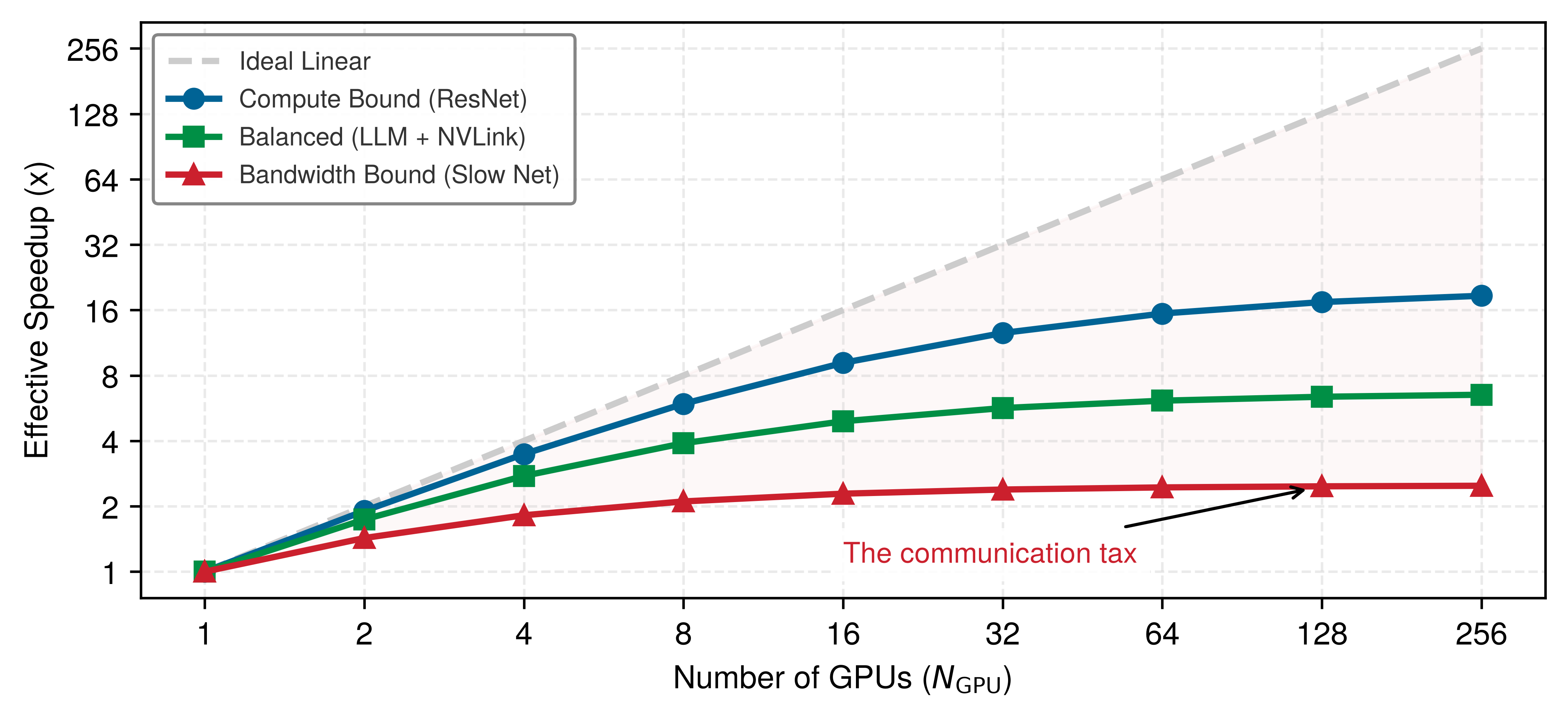
The red curve’s widening gap from the dashed ideal is the communication tax made visible; shrinking that gap is what the distributed strategies in section 1.6.1 exist to do.
Single-node multi-GPU training
Multi-GPU training within a single node, the scope of this book, predates large-scale distributed systems. AlexNet26 (Krizhevsky et al. 2012) famously split its model across two GTX 580 GPUs because the 3 GB memory limit made the network too large to train on one GPU. The split also made cross-GPU connectivity an architectural choice. This single-node, multi-GPU configuration remains a useful entry point because it introduces the core parallelism strategies without the complexity of network communication.
26 AlexNet (2012): The paper reports 60M parameters and a 3 GB single-GPU ceiling, but does not attribute the limit to one memory component. Its model-parallel design placed roughly half the kernels on each GPU and allowed communication only in selected layers, explicitly trading memory capacity against communication.
Krizhevsky, Alex, Ilya Sutskever, and Geoffrey E. Hinton. 2012. “ImageNet Classification with Deep Convolutional Neural Networks.” Advances in Neural Information Processing Systems (NeurIPS) 25.
The two foundational strategies, data parallelism and model parallelism, represent fundamentally different partitioning choices: data parallelism replicates the model and partitions data, while model parallelism partitions model state or computation. This distinction determines memory requirements, communication patterns, and scaling behavior.
Data parallelism
Data parallelism replicates the entire model on each GPU, with each processing different batches. After computing gradients locally, GPUs synchronize via gradient averaging. Figure 16 shows the data flow: input data splits into nonoverlapping batches, each accelerator computes forward and backward passes independently, then gradients aggregate before updating the shared model.
\begin{tikzpicture}[font=\small\sffamily]
\tikzset{
 Box/.style={draw=none,minimum width=41mm, minimum height=20mm, node distance=20mm and -16mm},
 Arr/.style={-{Triangle[width=10pt,length=8pt]}, line width=5pt,cyan!40,shorten >=1pt, shorten <=2pt},
 Box2/.style={align=flush center, inner xsep=2pt,draw=none,
  font=\footnotesize\sffamily, line width=0.75pt, fill=OrangeL!30, text width=41mm,
    minimum width=36mm, minimum height=7mm},
  Box3/.style = {Box2,draw=none,fill=cyan!10},
  Box4/.style = {Box2,draw=none,fill=GreenFill!60},
  Box5/.style = {Box2,draw=none,fill=magenta!10},
  LineA/.style = {violet!60,{Circle[line width=1.0pt,fill=white,length=5.5pt]}-,line width=1.5pt,shorten <=-3pt},
  Arr/.style={-{Triangle[width=9pt,length=7pt]}, line width=3pt,black!40,shorten >=1pt, shorten <=2pt},
  Txt/.style = {font=\footnotesize\sffamily,black!80,align=center}
}

\tikzset{mycylinder/.style={cylinder, shape border rotate=90, aspect=1.3, draw, fill=white,
minimum width=25mm,minimum height=11mm,line width=\Linewidth,node distance=-0.15},
pics/dataP/.style = {
        code = {
        \pgfkeys{/channel/.cd, #1}
\begin{scope}[local bounding box=STREAMING,scale=\scalefac, every node/.append style={transform shape}]
\node[mycylinder,fill=\filllcolor!50] (A) {};
\node[mycylinder, above=of A,fill=\filllcolor!50] (B) {};
\node[mycylinder, above=of B,fill=\filllcolor!10] (C) {};
\fill[\filllcolor!50!black]($(C.west)!0.12!(C.east)$)circle(3pt);
\fill[\filllcolor!50!black]($(B.west)!0.12!(B.east)$)circle(3pt);
\fill[\filllcolor!50!black]($(A.west)!0.12!(A.east)$)circle(3pt);
%
\draw[draw=\drawcolor,line width=2.5*\Linewidth](B.east)--++(17mm,0);
\node[draw=\drawcolor,line width=\Linewidth,minimum width=9mm,fill=white,minimum height=22mm](BD)at($(B.east)+(8mm,0)$){};
\node[draw=\drawcolor,line width=\Linewidth,minimum width=5mm,minimum height=8mm,fill=white](BDM)at($(BD.east)+(5mm,0)$){};
\node[circle,draw=orange,line width=\Linewidth,minimum size=5mm]at($(BD.north)!0.2!(BD.south)$){};
\node[rectangle,draw=blue,line width=\Linewidth,minimum size=5mm]at($(BD.north)!0.5!(BD.south)$){};
\node[circle,draw=green,line width=\Linewidth,minimum size=5mm]at($(BD.north)!0.8!(BD.south)$){};
\end{scope}
     }
  }
}
%CPU3
\tikzset{%
 pics/cpu3/.style = {
        code = {
        \pgfkeys{/channel/.cd, #1}
\begin{scope}[local bounding box=CHIP,scale=\scalefac, every node/.append style={transform shape}]
\node[fill=\filllcolor,draw=\drawcolor,minimum width=8mm, minimum height=8mm,inner sep=0pt,
            rounded corners=1pt,line width=2*\Linewidth,outer sep=2pt] (C1) {};
\foreach \x in {0.2,0.5,0.8}{
\draw[line width=1.3*\Linewidth,draw=\drawcolor,
-{Circle[fill=white,length=4.5pt]}]($(C1.north west)!\x!(C1.south west)$)--++(-3mm,0);
}
\foreach \x in {0.2,0.5,0.8}{
\draw[line width=1.3*\Linewidth,draw=\drawcolor,
-{Circle[fill=white,length=4.5pt]}]($(C1.north east)!\x!(C1.south east)$)--++(3mm,0);
}
%dole
\foreach \x in {0.2,0.5,0.8}{
\draw[line width=1.3*\Linewidth,draw=\drawcolor,
-{Circle[fill=white,length=4.5pt]}]($(C1.south west)!\x!(C1.south east)$)--++(0,-3mm);
}
  \draw[draw=\drawcolor,,-{Triangle[width=3.5pt,length=4pt]}, shorten >=-1pt,line width=1.1*\Linewidth,]
  ($(C1.north)+(2mm,2.25mm)$)+(180:1.75mm) arc (180:490:1.75mm);
% \draw[draw=\drawcolor,-{Triangle[width=3.5pt,length=4pt]}, shorten >=-1pt,line width=1.1*\Linewidth,]
%($(C1.south)+(0mm,-2.5mm)$) +(90:1.75mm)arc (90:380:1.75mm);
 \end{scope}
     }
  }
}
%data folder with arrws
\tikzset{%
 pics/arrowD/.style = {
        code = {
        \pgfkeys{/channel/.cd, #1}
\begin{scope}[local bounding box=DATAFOLDER,scale=\scalefac, every node/.append style={transform shape},
LinE/.style={\filllcirclecolor,line width=3.0pt,
{{Triangle[width=1.5*5pt,length=2.0*5pt]}-},shorten <=3pt,shorten >=1pt}
]
\node[fill=\filllcolor,circle,inner sep=1pt,minimum size=7mm](C1R){};
\draw[LinE](C1R.south)--++(270:2);
\draw[LinE](C1R.north)--++(270:-2);
\draw[LinE](C1R.west)--++(0:-2);
\draw[LinE](C1R.east)--++(0:2);
 \end{scope}
     }
  }
}
\tikzset{%
 pics/stackedA/.style = {
        code = {
        \pgfkeys{/channel/.cd, #1}
\begin{scope}[local bounding box=FUNNEL,scale=\scalefac, every node/.append style={transform shape}]
%plats
\draw[fill=\filllcirclecolor,line width=\Linewidth,draw=\drawcolor](0,-0.4)--(-0.67,-0.07)--(0,0.27)--(0.67,-0.07)--cycle;
\draw[fill=\filllcolor,line width=\Linewidth,draw=\drawcolor](0,-0.2)--(-0.67,0.13)--(0,0.47)--(0.67,0.13)--cycle;
\draw[fill=\filllcirclecolor,line width=\Linewidth,draw=\drawcolor](0,0)--(-0.67,0.33)--(0,0.67)--(0.67,0.33)--cycle;
\draw[fill=\filllcolor,line width=\Linewidth,draw=\drawcolor](0,0.2)--(-0.67,0.53)--(0,0.87)--(0.67,0.53)--cycle;
\draw[fill=\filllcirclecolor,line width=\Linewidth,draw=\drawcolor](0,0.4)--(-0.67,0.73)--(0,1.07)--(0.67,0.73)--cycle;
\node[draw=none,circle,minimum size=20mm](SREDI)at(0,0.33){};
\def\Rad{10mm}
 \draw[draw=mygreen,-{Triangle[width=3.5pt,length=6pt]}, shorten >=-1pt,line width=1.25*\Linewidth,]
(SREDI)+(100:\Rad) arc (100:260:\Rad);
 \draw[draw=myorange,-{Triangle[width=3.5pt,length=6pt]}, shorten >=-1pt,line width=1.25*\Linewidth,]
(SREDI)+(280:\Rad)arc (280:440:\Rad);
\end{scope}
     }
  }
}
\pgfkeys{
  /channel/.cd,
   Depth/.store in=\Depth,
  Height/.store in=\Height,
  Width/.store in=\Width,
  filllcirclecolor/.store in=\filllcirclecolor,
  filllcolor/.store in=\filllcolor,
  drawcolor/.store in=\drawcolor,
  drawcircle/.store in=\drawcircle,
  scalefac/.store in=\scalefac,
  Linewidth/.store in=\Linewidth,
  picname/.store in=\picname,
  filllcolor=BrownLine,
  filllcirclecolor=violet!20,
  drawcolor=black,
  drawcircle=violet,
  scalefac=1,
  Linewidth=0.5pt,
  Depth=1.3,
  Height=0.8,
  Width=1.1,
  picname=C
}

%Input Data
\node[Box, fill=white](B1){};
\pic[shift={(-0.56,-0.6)}] at  (B1){dataP={scalefac=0.56,picname=1,filllcirclecolor=violet!20,filllcolor=BlueLine, Linewidth=0.7pt}};
\draw[mybrown,line width=1.5pt](B1.south west)--coordinate(1S1)(B1.south east);
\node[Box2,anchor=north,below= 0.2 of B1](T1){Input Data};
%%%%%%%%%%%%%%%%%%%%%
%second row
%%%%%%%%%%%%%%%%%%%%%
%Batch 2
\node[Box, fill=white,below left=1.7 and -1.7  of B1](2B2){};
\pic[shift={(0,0)}] at  (2B2){cpu3={scalefac=1.1,drawcolor=BlueLine, filllcolor=white, Linewidth=1pt}};
\draw[mybrown,line width=1.5pt](2B2.south west)--coordinate(2S2)(2B2.south east);
\node[Box3,anchor=north,below= 0.2 of 2B2](2T2){Batch 2\\ GPU 2
Forward \& Backward};
%Batch 3
\node[Box, fill=white,below right=1.7 and -1.7  of B1](2B3){};
\pic[shift={(0,0)}] at  (2B3){cpu3={scalefac=1.1,drawcolor=BlueLine, filllcolor=white, Linewidth=1pt}};
\draw[mybrown,line width=1.5pt](2B3.south west)--coordinate(2S3)(2B3.south east);
\node[Box3,anchor=north,below= 0.2 of 2B3](2T3){Batch 3\\ GPU 3
Forward \& Backward};
%Batch 4
\node[Box, fill=white, right=0.6 of 2B3](2B4){};
\pic[shift={(0,0)}] at  (2B4){cpu3={scalefac=1.1,drawcolor=BlueLine, filllcolor=white, Linewidth=1pt}};
\draw[mybrown,line width=1.5pt](2B4.south west)--coordinate(2S4)(2B4.south east);
\node[Box3,anchor=north,below= 0.2 of 2B4](2T4){Batch 4\\ GPU 4
Forward \& Backward};
%Batch 1
\node[Box, fill=white, left=0.6 of 2B2](2B1){};
\pic[shift={(0,0)}] at  (2B1){cpu3={scalefac=1.1,drawcolor=BlueLine, filllcolor=white, Linewidth=1pt}};
\draw[mybrown,line width=1.5pt](2B1.south west)--coordinate(2S1)(2B1.south east);
\node[Box3,anchor=north,below= 0.2 of 2B1](2T1){Batch 1\\ GPU 1
Forward \& Backward};
%%%%%%%%%%%%%%%%%%%%%
%third row
%%%%%%%%%%%%%%%%%%%%%
%Gradient Sync / All-Reduce
\node[Box, fill=white,below =5.7 of B1](3B1){};
\pic[shift={(0,0.1)},rotate=45] at  (3B1){arrowD={scalefac=0.45,picname=1,Linewidth=1.0pt,
 filllcolor=mygreen,drawcolor=BrownLine,filllcirclecolor=mypurple}};
\draw[mybrown,line width=1.5pt](3B1.south west)--coordinate(3S1)(3B1.south east);
\node[Box4,anchor=north,below= 0.2 of 3B1](3T1){Gradient Sync / AllReduce};
%%%%%%%%%%%%%%%%%%%%%
%fourth row
%%%%%%%%%%%%%%%%%%%%%
%Model Update
\node[Box, fill=white,below =1.6 of 3B1](4B1){};
\pic[shift={(0,-0.24)}] at  (4B1){stackedA={scalefac=0.9,Linewidth=1.0pt,
 filllcolor=cyan!90,drawcolor=none,filllcirclecolor=myred!35}};
\draw[mybrown,line width=1.5pt](4B1.south west)--coordinate(4S1)(4B1.south east);
\node[Box5,anchor=north,below= 0.2 of 4B1](4T1){Model Update};
%
%fitting
\begin{scope}[on background layer]
%\node[draw=brown,inner sep=3mm,dashed,line width=1pt,fit=(T1)(1S1)(B1)](F1){};
%\node[anchor=south east,font=\small\sffamily\bfseries]at(F1.north east){ML System Implementations};
%
\node[draw=myblue,inner sep=3mm,inner ysep=1mm,yshift=-0.25mm,
dashed,line width=1pt,fit=(2T1)(2T4)(2B3)](F2){};
%\node[anchor=south east,font=\small\sffamily\bfseries]at(F2.north east){Core System Principles};
%
%\node[draw=mygreen,inner sep=3mm,dashed,line width=1pt,fit=(3T1)(3B1)](F3){};
%\node[anchor=south east,font=\small\sffamily\bfseries]at(F3.north east){System Considerations};
%
\end{scope}
%arrows
\draw[Arr](T1)--(F2);
\draw[Arr](F2)--(3B1);
\draw[Arr](3T1)--(4B1);
\end{tikzpicture}Data parallelism’s appeal lies in its simplicity and efficiency. Each GPU runs the same forward-backward computation on different data, and replicas agree on gradients before updating parameters. Modern implementations bucket and overlap reductions with backpropagation. This makes data parallelism the natural first strategy when models fit in GPU memory. PyTorch’s DistributedDataParallel and TensorFlow’s MirroredStrategy automate synchronization, keeping the programming model close to single-GPU training despite per-iteration communication.
Unsharded data parallelism has a hard constraint: every GPU holds a complete model replica and ordinarily its local optimizer state. A 7-billion-parameter model uses 14 GB for FP16 weights alone, before gradients, optimizer states, or activations. Sharded data parallelism (such as the Zero Redundancy Optimizer, or ZeRO) distributes that state across devices: ZeRO-1 shards optimizer states, ZeRO-2 shards gradients, and ZeRO-3 (or FSDP) shards model parameters; otherwise, a model that exceeds local memory requires pipeline or tensor partitioning.
Model parallelism
Model parallelism partitions the model itself across GPUs, which becomes necessary when the model exceeds single-GPU memory. AlexNet used a simple form: certain layers resided on GPU 1, others on GPU 2, with activations passing between them. Figure 17 shows the forward and backward paths: data moves through model partitions on different devices, with gradients flowing backward during training.
\begin{tikzpicture}[line join=round,font=\sffamily\small]
\tikzset{%
  Box/.style={align=flush center,
    inner xsep=2pt,
    node distance=0.65,
    draw=VioletLine,
    line width=0.75pt,
    fill=VioletL2!13,
    %text width=35mm,
    minimum width=35mm, minimum height=15mm
  },
  Box2/.style={Box, draw=myblue, fill=myblue!03,
  },
  LineA/.style={mybrown!50,line width=1.5pt,{-{Triangle[width=1.0*5pt,length=1.0*8pt]}},
  shorten <=2pt,shorten >=2pt},
  LineAA/.style={myorange!50,line width=1.5pt,{-{Triangle[width=1.0*5pt,length=1.0*8pt]}},
  shorten <=2pt,shorten >=2pt},
  LineA2/.style={black!25,line width=1.25pt,{-{Triangle[width=1.0*5pt,length=1.0*8pt]}},
  shorten <=0pt,shorten >=0pt},
}

\tikzset {
pics/output/.style = {
        code = {
        \pgfkeys{/channel/.cd, #1}
\begin{scope}[local bounding box=CLO,scale=\scalefac,, every node/.append style={transform shape}]
\node[draw=\drawcolor,line width=\Linewidth,rounded corners=2pt,
rectangle,minimum width=10mm,minimum height=13mm](REC){};
\node[rectangle,draw=none,fill=white,minimum width=10.5mm,minimum height=5mm,anchor=west]{};
\node[single arrow, draw=orange,fill=orange,inner sep=2pt,\filllcirclecolor,
      minimum width = 5mm, single arrow head extend=3pt,
      minimum height=10mm,anchor=west,
      rotate=0]at(0,0) {};
\end{scope}
}
}
}
 \tikzset{mycylinder/.style={cylinder, shape border rotate=90, aspect=1.3, draw, fill=white,
minimum width=25mm,minimum height=11mm,line width=\Linewidth,node distance=-0.15},
pics/data/.style = {
        code = {
        \pgfkeys{/channel/.cd, #1}
\begin{scope}[local bounding box=STREAMING,scale=\scalefac, every node/.append style={transform shape}]
\node[mycylinder,fill=\filllcolor!50] (A) {};
\node[mycylinder, above=of A,fill=\filllcolor!30] (B) {};
\node[mycylinder, above=of B,fill=\filllcolor!10] (C) {};
\fill[\filllcolor!50!black]($(C.west)!0.12!(C.east)$)circle(3pt);
\fill[\filllcolor!50!black]($(B.west)!0.12!(B.east)$)circle(3pt);
\fill[\filllcolor!50!black]($(A.west)!0.12!(A.east)$)circle(3pt);
 \end{scope}
     }
  }
}
%CPU3
\tikzset{%
 pics/cpu3/.style = {
        code = {
        \pgfkeys{/channel/.cd, #1}
\begin{scope}[local bounding box=CHIP,scale=\scalefac, every node/.append style={transform shape}]
\node[fill=\filllcolor,draw=\drawcolor,minimum width=10mm, minimum height=10mm,inner sep=0pt,
            rounded corners=1pt,line width=2*\Linewidth,outer sep=2pt] (C1) {};
\foreach \x in {0.2,0.5,0.8}{
\draw[line width=1.3*\Linewidth,draw=\drawcolor,
-{Circle[fill=white,length=3.5pt]}]($(C1.north west)!\x!(C1.south west)$)--++(-3mm,0);
}
\foreach \x in {0.2,0.5,0.8}{
\draw[line width=1.3*\Linewidth,draw=\drawcolor,
-{Circle[fill=white,length=3.5pt]}]($(C1.north east)!\x!(C1.south east)$)--++(3mm,0);
}
%dole
\foreach \x in {0.2,0.5,0.8}{
\draw[line width=1.3*\Linewidth,draw=\drawcolor,
-{Circle[fill=white,length=3.5pt]}]($(C1.south west)!\x!(C1.south east)$)--++(0,-3mm);
}
%gore
\foreach \x in {0.2,0.5,0.8}{
\draw[line width=1.3*\Linewidth,draw=\drawcolor,
-{Circle[fill=white,length=3.5pt]}]($(C1.north west)!\x!(C1.north east)$)--++(0,3mm);
}
 \end{scope}
     }
  }
}
\pgfkeys{
  /channel/.cd,
   Depth/.store in=\Depth,
  Height/.store in=\Height,
  Width/.store in=\Width,
  filllcirclecolor/.store in=\filllcirclecolor,
  filllcolor/.store in=\filllcolor,
  drawcolor/.store in=\drawcolor,
  drawcircle/.store in=\drawcircle,
  scalefac/.store in=\scalefac,
  Linewidth/.store in=\Linewidth,
  picname/.store in=\picname,
  filllcolor=BrownLine,
  filllcirclecolor=violet!20,
  drawcolor=red,
  drawcircle=violet,
  scalefac=1,
  Linewidth=0.5pt,
  Depth=0.2,
  Height=0.5,
  Width=0.25,
  picname=C
}

%Input Data
\node[Box](B1){};
\coordinate(GO1)at($(B1.north west)!0.38!(B1.north east)$);
\coordinate(T1)at($(GO1)!0.5!(B1.south east)$);
\coordinate(I1)at($(B1.west)!0.21!(B1.east)$);
\node[align=center]at(T1){Input Data};
\node[Box,fill=none]{};
\pic[shift={(0,-0.38)}] at  (I1){data={scalefac=0.35,picname=1,filllcolor=mygreen, Linewidth=0.6pt}};
%Device 1
\node[Box2,right=of B1](B2){};
\coordinate(GO2)at($(B2.north west)!0.38!(B2.north east)$);
\coordinate(T2)at($(GO2)!0.5!(B2.south east)$);
\coordinate(I2)at($(B2.west)!0.21!(B2.east)$);
\node[align=center]at(T2){Device 1 \\ Layers 1-16};
\node[Box,fill=none]{};
\pic[shift={(0,0)}] at  (I2){cpu3={scalefac=0.67,drawcolor=BrownLine, filllcolor=white, Linewidth=0.75pt}};
%Device 2
\node[Box2,right=of B2](B3){};
\coordinate(GO3)at($(B3.north west)!0.38!(B3.north east)$);
\coordinate(T3)at($(GO3)!0.5!(B3.south east)$);
\coordinate(I3)at($(B3.west)!0.21!(B3.east)$);
\node[align=center]at(T3){Device 2\\ Layers 17-32};
\node[Box,fill=none]{};
\pic[shift={(0,0)}] at  (I3){cpu3={scalefac=0.67,drawcolor=BrownLine, filllcolor=white, Linewidth=0.75pt}};
%Device 3
\node[Box2,right=of B3](B4){};
\coordinate(GO4)at($(B4.north west)!0.38!(B4.north east)$);
\coordinate(T4)at($(GO4)!0.5!(B4.south east)$);
\coordinate(I4)at($(B4.west)!0.21!(B4.east)$);
\node[align=center]at(T4){Device 3\\ Layers 33-48};
\node[Box,fill=none]{};
\pic[shift={(0,0)}] at  (I4){cpu3={scalefac=0.67,drawcolor=BrownLine, filllcolor=white, Linewidth=0.75pt}};
%Output
\node[Box,right=of B4](B5){};
\coordinate(GO5)at($(B5.north west)!0.38!(B5.north east)$);
\coordinate(T5)at($(GO5)!0.5!(B5.south east)$);
\coordinate(I5)at($(B5.west)!0.21!(B5.east)$);
\node[align=center]at(T5){Output};
\node[Box,fill=none]{};
\pic[shift={(0,0)}] at  (I5){output={scalefac=0.7,filllcirclecolor=orange!80,drawcolor=BlueLine,
 filllcirclecolor=mygreen, Linewidth=5.0pt}};
%
\node[inner xsep=0pt,above=4mm of B1.north,anchor=south ](GT1){Forward pass};
\node[inner xsep=0pt,above=4.3mm of B3.north,anchor=south](GT2){Activations};
\node[inner xsep=0pt,above=4mm of B5.north,anchor=south ](GT3){Output};
\draw[LineA](GT1)--(GT2);
\draw[LineA](GT2)--(GT3);
%
\node[inner xsep=0pt,rectangle,minimum height=4mm,draw=none,
below=4mm of B1.south,anchor=north](DT1){Backward pass};
\node[inner xsep=0pt,rectangle,minimum height=4mm,draw=none,
below=4.3mm of B3.south,anchor=north](DT2){Gradients};
\node[inner xsep=0pt,rectangle,minimum height=4mm,draw=none,
below=4mm of B5.south,anchor= north](DT3){Loss gradient};
\draw[LineAA](DT3.west)--(DT2.east);
\draw[LineAA](DT2.west)--(DT1.east);
%
\foreach \i  in {1,2,3,4}{
\pgfmathtruncatemacro{\x}{\i + 1} %
\draw[LineA2](B\i)--(B\x);
}
\end{tikzpicture}Systems Perspective 1.7: Data vs. model parallelism
When a selected workload is partitioned across \(N_{\text{GPU}}\) devices, the split may divide examples, model state, layers, or tensor operations. For a model with parameters \(P\) and batch size \(B\), data and model parallelism provide two starting points.
Data parallelism (split the batch): For a fixed global batch, each of \(N_{\text{GPU}}\) workers processes about \(1/N_{\text{GPU}}\) of the examples, but every worker holds a model replica and ordinarily its associated training state. Dense gradient communication is proportional to \(P\) per update. Scaling departs from the ideal as local batches shrink or synchronization and input costs grow.
Model parallelism (split model computation): Each accelerator stores and computes a portion of the model. An even partition may approach \(P/N_{\text{GPU}}\) parameters per worker, but embeddings, buffers, imbalance, and replicated state alter that estimate. Communication depends on the partition: layerwise pipeline parallelism exchanges activations at stage boundaries, while tensor parallelism performs collectives within partitioned layers.
Systems insight: Data parallelism is the simplest candidate when the complete training state fits per worker and more throughput is needed. Model-state, pipeline, or tensor partitioning becomes necessary when it does not, often in combination with data parallelism.
When a model exceeds the memory capacity of a single accelerator, its depth can be partitioned across sequential devices. Examine the pipeline stage assignment in figure 18, observing how contiguous groups of transformer blocks map onto distinct devices across the execution chain.
\begin{tikzpicture}[font=\sffamily\small]

\tikzset{
  Box/.style={ inner xsep=2pt,
    node distance=1.4,
    draw=none,
    line width=0.5pt,,
    fill=none,
    minimum width=22mm, minimum height=10mm
  },
    LineA/.style={myblue!40,line width=3pt,{-{Triangle[width=1.0*6pt,length=1.0*8pt]}},shorten <=1pt,shorten >=1pt},
}
%CPU2
\tikzset{%
 pics/cpu3/.style = {
        code = {
        \pgfkeys{/channel/.cd, #1}
\begin{scope}[local bounding box=CHIP,scale=\scalefac, every node/.append style={transform shape}]
\node[fill=\filllcolor,draw=\drawcolor,minimum width=8mm, minimum height=8mm,inner sep=0pt,
            rounded corners=1pt,line width=2.5*\Linewidth,outer sep=2pt] (C1) {};
\foreach \x in {0.2,0.5,0.8}{
\draw[line width=1.3*\Linewidth,draw=\drawcolor,
-{Circle[fill=white,length=3.2pt]}]($(C1.north west)!\x!(C1.south west)$)--++(-3mm,0);
}
\foreach \x in {0.2,0.5,0.8}{
\draw[line width=1.1*\Linewidth,draw=\drawcolor,
-{Circle[fill=white,length=3.2pt]}]($(C1.north east)!\x!(C1.south east)$)--++(3mm,0);
}
%dole
\foreach \x in {0.2,0.5,0.8}{
\draw[line width=1.1*\Linewidth,draw=\drawcolor,
-{Circle[fill=white,length=3.2pt]}]($(C1.south west)!\x!(C1.south east)$)--++(0,-3mm);
}
%gore
\foreach \x in {0.2,0.5,0.8}{
\draw[line width=1.1*\Linewidth,draw=\drawcolor,
-{Circle[fill=white,length=3.2pt]}]($(C1.north west)!\x!(C1.north east)$)--++(0,3mm);
}
 \end{scope}
     }
  }
}
\tikzset{%
 pics/stackedS/.style = {
        code = {
        \pgfkeys{/channel/.cd, #1}
\begin{scope}[local bounding box=STACKED,scale=\scalefac, every node/.append style={transform shape}]
%plats

\draw[fill=\filllcolor,line width=\Linewidth,draw=\drawcolor](0,-0.2)--(-0.67,0.13)--(0,0.47)--(0.67,0.13)--cycle;
\draw[fill=\filllcirclecolor,line width=\Linewidth,draw=\drawcolor](0,0)--(-0.67,0.33)--(0,0.67)--(0.67,0.33)--cycle;
\draw[fill=\filllcolor,line width=\Linewidth,draw=\drawcolor](0,0.2)--(-0.67,0.53)--(0,0.87)--(0.67,0.53)--cycle;
\draw[fill=\filllcirclecolor,line width=\Linewidth,draw=\drawcolor](0,0.4)--(-0.67,0.73)--(0,1.07)--(0.67,0.73)--cycle;
\end{scope}
     }
  }
}
\pgfkeys{
  /channel/.cd,
   Depth/.store in=\Depth,
  Height/.store in=\Height,
  Width/.store in=\Width,
  filllcirclecolor/.store in=\filllcirclecolor,
  filllcolor/.store in=\filllcolor,
  drawcolor/.store in=\drawcolor,
  drawcircle/.store in=\drawcircle,
  scalefac/.store in=\scalefac,
  Linewidth/.store in=\Linewidth,
  picname/.store in=\picname,
  filllcolor=BrownLine,
  filllcirclecolor=cyan!40,
  drawcolor=black,
  drawcircle=violet,
  scalefac=1,
  Linewidth=0.5pt,
  Depth=1.3,
  Height=0.8,
  Width=1.1,
  picname=C
}
%device 1
\begin{scope}[local bounding box=D1,shift={($(0,0)+(0,0)$)}]
\node[Box](MM){};
\node[below=1pt of MM](T1){Blocks 1-6};
\pic[shift={(0,-0.35)}] at  (MM){stackedS={scalefac=0.8,Linewidth=1.0pt,
 filllcolor=cyan!90!black!40!,drawcolor=black,filllcirclecolor=orange}};
%
\node[below=3mm of T1,Box](DP){};
\node[below=1pt of DP](T2){GPU 1};
\pic[shift={(0,0)}] at  (DP){cpu3={scalefac=0.7, drawcolor=BlueLine, filllcolor=white, Linewidth=0.75pt}};

\scoped[on background layer]
\node[fit=(MM)(T1)(T2),draw=red,yshift=4mm,inner xsep=2mm,inner ysep=5mm,
fill=BackColor!10,draw=myolive](DD){};
\node[below=1pt of DD.north,font=\sffamily\bfseries\footnotesize]{Device 1};
\end{scope}
%device 2
\begin{scope}[local bounding box=D2,shift={($(0,0)+(4.5,0)$)}]
\node[Box](MM){};
\node[below=1pt of MM](T1){Blocks 7-12};
\pic[shift={(0,-0.35)}] at  (MM){stackedS={scalefac=0.8,Linewidth=1.0pt,
 filllcolor=cyan!90!black!40!,drawcolor=black,filllcirclecolor=orange}};
%
\node[below=3mm of T1,Box](DP){};
\node[below=1pt of DP](T2){GPU 2};
\pic[shift={(0,0)}] at  (DP){cpu3={scalefac=0.7, drawcolor=BlueLine, filllcolor=white, Linewidth=0.75pt}};

\scoped[on background layer]
\node[fit=(MM)(T1)(T2),draw=red,yshift=4mm,inner xsep=2mm,inner ysep=5mm,
fill=BackColor!10,draw=myolive](DD){};
\node[below=1pt of DD.north,font=\sffamily\bfseries\footnotesize]{Device 2};
\end{scope}
%device 3
\begin{scope}[local bounding box=D3,shift={($(0,0)+(9,0)$)}]
\node[Box](MM){};
\node[below=1pt of MM](T1){Blocks 13-18};
\pic[shift={(0,-0.35)}] at  (MM){stackedS={scalefac=0.8,Linewidth=1.0pt,
 filllcolor=cyan!90!black!40!,drawcolor=black,filllcirclecolor=orange}};
%
\node[below=3mm of T1,Box](DP){};
\node[below=1pt of DP](T2){GPU 3};
\pic[shift={(0,0)}] at  (DP){cpu3={scalefac=0.7, drawcolor=BlueLine, filllcolor=white, Linewidth=0.75pt}};

\scoped[on background layer]
\node[fit=(MM)(T1)(T2),draw=red,yshift=4mm,inner xsep=2mm,inner ysep=5mm,
fill=BackColor!10,draw=myolive](DD){};
\node[below=1pt of DD.north,font=\sffamily\bfseries\footnotesize]{Device 3};
\end{scope}
%device 4
\begin{scope}[local bounding box=D4,shift={($(0,0)+(13.5,0)$)}]
\node[Box](MM){};
\node[below=1pt of MM](T1){Blocks 19-24};
\pic[shift={(0,-0.35)}] at  (MM){stackedS={scalefac=0.8,Linewidth=1.0pt,
 filllcolor=cyan!90!black!40!,drawcolor=black,filllcirclecolor=orange}};
%
\node[below=3mm of T1,Box](DP){};
\node[below=1pt of DP](T2){GPU 4};
\pic[shift={(0,0)}] at  (DP){cpu3={scalefac=0.7, drawcolor=BlueLine, filllcolor=white, Linewidth=0.75pt}};

\scoped[on background layer]
\node[fit=(MM)(T1)(T2),draw=red,yshift=4mm,inner xsep=2mm,inner ysep=5mm,
fill=BackColor!10,draw=myolive](DD){};
\node[below=1pt of DD.north,font=\sffamily\bfseries\footnotesize]{Device 4};
\end{scope}

 \foreach \i [evaluate=\i as \t using int(\i+1)] in {1,2,3}{
\draw[LineA](D\i)--
node[above,pos=0.45,text=black!50,font=\sffamily
\fontsize{9pt}{7}\selectfont]{Activations}
(D\t);
}
\end{tikzpicture}Model parallelism’s challenge is idle time. While Device 1 computes layers 1–6, Devices 2–4 sit idle waiting for activations. During the backward pass, the problem reverses: Device 4 computes first while others wait. This “pipeline bubble” means naive model parallelism can waste much of the available accelerator time even with careful partitioning. Pipeline parallelism addresses this inefficiency, as the discussion of distributed strategies demonstrates.
Within a node, GPUs may communicate through high-bandwidth links such as NVLink27 (up to 900 GB/s aggregate bidirectional bandwidth for the represented H100 configuration). Effective collective bandwidth depends on topology and contention and is lower than a raw aggregate link specification. Data parallelism communicates gradients, while layerwise model parallelism communicates activations at partition boundaries. Choosing a strategy requires comparing its compute, memory, and communication on the actual topology.
27 NVLink: NVIDIA’s high-bandwidth GPU interconnect. Its topology and generation determine the bandwidth available between a particular pair of GPUs and to collective operations. A parallelism strategy helps only when its communication and synchronization cost is smaller than the useful time it saves.
Scaling beyond a single node
When single-node multi-GPU training remains insufficient, distributed training extends across machines. This introduces a slower or more contended communication tier and makes host, switch, routing, and fault behavior part of training performance. The bandwidth gap matters because synchronous data-parallel updates turn gradient reduction into a recurring data-movement problem.
Systems Perspective 1.8: The physics of synchronization
Recall the energy-movement invariant from Data Engineering: data movement can cost substantially more energy and time than nearby arithmetic. In distributed training, this asymmetry contributes to the communication tax.
Synchronizing gradients across GPUs moves megabytes over a network or PCIe every few milliseconds. Uncovered communication lowers utilization, while communication energy raises the run’s energy budget; these are distinct costs. Mixed precision (section 1.5.3) and gradient compression reduce bytes through narrower formats, sparsity, quantization, or encoding, addressing both pressures.
Within a node, fast links can make it possible to overlap part of gradient synchronization with backward computation. Crossing node boundaries adds another fabric whose effective bandwidth and latency depend on topology and collective implementation. In synchronous data parallelism, AllReduce28 aggregates gradients across workers; at sufficient scale, its uncovered communication time can dominate the step.
28 AllReduce: A collective communication primitive that sums data across all devices and distributes the result back to each device. Ring AllReduce is one common implementation: devices pass gradient shards around a logical ring so each participant sends and receives bounded chunks rather than a full copy of every gradient tensor at once. This is the communication primitive that makes large data-parallel training practical, but its detailed cost model belongs with distributed training.
A short calculation shows how quickly the inter-node fabric becomes the binding constraint.
Napkin Math 1.10: The network wall
Problem: A team scales training to 8 GPUs, one per node, connected by a 100 Gbps fabric. Is the network the bottleneck?
Mechanism: For a 7B-parameter model with FP16 gradients:
- Gradient size (FP16): 14 GB per step.
- AllReduce cost: Ring AllReduce passes gradient shards around a logical ring, so each worker ends up sending nearly two full copies of the gradient: \(2(N_{\text{GPU}}-1)/N_{\text{GPU}}\), which equals 1.75× for 8 GPUs. That gives 1.75 \(\times\) 14 GB = 24.5 GB total.
- Bandwidth-only lower bound: At 12.5 GB/s per worker on the 100 Gbps fabric, synchronization latency is \(T_{\text{comm}} = D_{\text{comm}} / \text{BW}_{\text{net}} =\) 24.5 GB / 12.5 GB/s \(=\) 1.96 s.
- Compute comparison: If the nonoverlapped forward and backward work takes \(T_{\text{compute}} \approx\) 1 s, communication latency \(T_{\text{comm}} \approx\) 1.96 s dominates.
Systems lesson: The network becomes a wall when \(T_{\text{comm}} > T_{\text{compute}}\), causing accelerator efficiency \(\eta_{\text{hw}} = \frac{T_{\text{compute}}}{T_{\text{compute}} + T_{\text{comm}}}\) to plummet to about 33.8 percent. Mitigations include gradient compression (reducing \(D_{\text{comm}}\)), ring AllReduce primitives (Sergeev and Balso 2018), and hierarchical topologies that confine high-frequency transfers to fast intra-node links (NVLink at 900 GB/s vs 12.5 GB/s inter-node).
Sergeev, Alexander, and Mike Del Balso. 2018. “Horovod: Fast and Easy Distributed Deep Learning in TensorFlow.” CoRR abs/1802.05799.
29 GPipe (2019): GPipe implements the described microbatching strategy, staggering execution to fill the idle “bubbles” in naive model parallelism and thus boost utilization (Huang et al. 2019). The key trade-off it manages is increased memory for storing the activations of multiple in-flight microbatches. It preserves large-batch training dynamics by accumulating gradients before the weight update; the paper reports almost linear Transformer throughput scaling when the micro-batch count is at least four times the number of partitions.
Huang, Y., Y. Cheng, A. Bapna, O. Firat, D. Chen, M. X. Chen, H. Lee, et al. 2019. “GPipe: Efficient Training of Giant Neural Networks Using Pipeline Parallelism.” Advances in Neural Information Processing Systems (NeurIPS) 32: 103–12.
Once training crosses the node boundary, the strategy must match communication frequency to available bandwidth. Pipeline parallelism addresses idle time in layerwise partitioning through micro-batching. While one stage processes a later micro-batch, the next stage can process an earlier one. The schedule determines how many micro-batch activations each stage must retain until their backward computations; this can increase memory, but not every device stores the full model-wide activation footprint for every in-flight micro-batch. GPipe29 and PipeDream developed influential schedules for this trade-off (Huang et al. 2019; Narayanan et al. 2019).
Tensor parallelism takes a finer-grained approach: rather than assigning whole layers to devices, it splits individual operations across devices. (Sequence parallelism extends this principle by sharding activation tensors along the sequence dimension across devices during long-sequence transformer training.) Consider a transformer’s feed-forward layer with a large matrix multiplication \(\mathbf{Y} = \mathbf{X}\mathbf{W}\). Tensor parallelism splits the weight matrix \(\mathbf{W}\) column-wise across GPUs, so each accelerator computes a portion of the output. The results are then gathered to form the complete output. This strategy is particularly effective for the massive attention and feed-forward layers in large transformers, where a single operation may involve matrices too large for one GPU’s memory. Megatron-LM demonstrated that tensor parallelism enables training models with billions of parameters by distributing individual attention heads and feed-forward blocks across devices (Shoeybi et al. 2019).
Shoeybi, Mohammad, Mostofa Patwary, Raul Puri, Patrick LeGresley, Jared Casper, and Bryan Catanzaro. 2019. “Megatron-LM: Training Multi-Billion Parameter Language Models Using Model Parallelism.” arXiv Preprint arXiv:1909.08053.
Hybrid strategies combine these approaches because each has different scaling characteristics. Table 20 gives a topology-dependent heuristic: place the most frequent communication on the fastest links and less frequent synchronization on slower tiers.
The placement rule is not arbitrary; it maps communication frequency to the fastest available bandwidth tier.
| Strategy | Typical placement | Communication pattern |
|---|---|---|
| Tensor parallelism | Within a node | Frequent communication that exploits NVLink’s high bandwidth |
| Pipeline parallelism | Across nodes within a rack | Moderate communication at layer boundaries |
| Data parallelism | Across racks | Gradient synchronization once per iteration |
Data-parallel systems also rely on collective operations such as AllReduce to combine gradients across devices. The implementation details of collective algorithms, parameter-server and peer-to-peer communication patterns, fault tolerance mechanisms, and scaling-efficiency analysis for training runs spanning thousands of GPUs constitute a specialized domain that builds on the foundations established here.
The evolution of training infrastructure
The parallelism strategies in section 1.6.1 and section 1.6.2 are one endpoint of a longer infrastructure progression. Training systems took this form because computing infrastructure evolved through four distinct eras, each shaped by dominant workloads. Figure 19 situates those eras on a timeline, while table 21 compares their workloads, memory patterns, and processing models.
Neural-network training combines requirements from multiple predecessors. Like HPC, it uses substantial floating-point throughput; like warehouse-scale computing, large runs require coordination and fault handling across machines. Many current large-scale jobs use synchronous collectives each optimizer step, but asynchronous parameter servers, local-update methods, and other synchronization schemes also exist. The recurring high-volume communication of common synchronous training recipes helped motivate accelerator clusters with high-bandwidth interconnects and software stacks optimized for collective communication.
\begin{tikzpicture}[font=\small\sf,node distance=0pt,xscale=2]
\tikzset{
  Box/.style={inner xsep=2pt, draw=black!80, line width=0.75pt,
    fill=black!10, anchor=south, rounded corners=2pt,
    font=\sf\footnotesize, align=center, minimum height=5mm},
}
\definecolor{col1}{RGB}{240,240,255}
\definecolor{col2}{RGB}{255, 255, 205}
\def\du{199mm}
\def\vi{15mm}
\node[fill=green!10,draw=none,minimum width=\du,
name path=G4,anchor=south west, minimum height=\vi](B1)at(-19.0mm,3mm){};
\node[right=2mm of B1.west,anchor=west,align=left]{AI Hypercomputing\\ Era};
\node[fill=col2,draw=none,minimum width=\du,
name path=G3,anchor=south west, minimum height=\vi](Z)at(B1.north west){};
\node[right=2mm of Z.west,anchor=west,align=left]{Warehouse Scale\\ Computing};
\node[fill=red!10,draw=none,minimum width=\du,
anchor=south west, minimum height=\vi](B2)at (Z.north west){};
\node[right=2mm of B2.west,anchor=west,align=left]{High-Performance\\ Computing};
\node[fill=col1,draw=none,minimum width=\du,
name path=G1,anchor=south west, minimum height=\vi](V)at(B2.north west){};
\node[right=2mm of V.west,anchor=west,align=left]{Mainframe};
\def\hi{6.75}
\draw[thick,name path=V1](0mm,0)node[below]{1950}--++(90:\hi);
\draw[thick,name path=V2](10mm,0)node[below]{1960}--++(90:\hi);
\draw[thick,name path=V3](20mm,0)node[below]{1970}--++(90:\hi);
\draw[thick,name path=V4](30mm,0)node[below]{1980}--++(90:\hi);
\draw[thick,name path=V5](40mm,0)node[below]{1990}--++(90:\hi);
\draw[thick,name path=V6](50mm,0)node[below]{2000}--++(90:\hi);
\draw[thick,name path=V7](60mm,0)node[below]{2010}--++(90:\hi);
\draw[thick,name path=V8](70mm,0)node[below]{2020}--++(90:\hi);
\def\fa{2}
\path [name intersections={of=V1 and G1,by={A,B}}];
\node[Box, minimum width=20mm, anchor=south west, xshift=-\fa*5mm]at([yshift=1pt]B){ENIAC};
\path [name intersections={of=V3 and G1,by={C,D}}];
\node[Box, minimum width=20mm, anchor=north west, xshift=-\fa*6mm]at([yshift=-1pt]C){IBM\\ System/360};
\node[Box, minimum width=40mm, anchor=north west, xshift=-\fa*6mm]at([yshift=-1pt]D){CDC 6600};
\path [name intersections={of=V4 and G3,by={E,F}}];
\node[Box, minimum width=30mm, anchor=south west, xshift=-\fa*4mm]at([yshift=1pt]E){Cray-1};
\path [name intersections={of=V6 and G3,by={G,H}}];
\node[Box, minimum width=20mm, anchor=north west, xshift=0mm]at([yshift=-1pt]G){Google Data\\ Centers};
\path [name intersections={of=V7 and G3,by={I,J}}];
\node[Box, minimum width=22mm, anchor=south west, xshift=-\fa*5mm]at([yshift=1pt]J){AWS};
\path [name intersections={of=V8 and G4,by={K,L}}];
\node[Box, minimum width=20mm, anchor=north west, xshift=-\fa*5mm]at([yshift=-1pt]K){NVIDIA GPU};
\node[Box,minimum width=2mm, anchor=south, xshift=-\fa*0mm]at([yshift=1pt]L){};
\node[minimum width=20mm, anchor=south west, xshift=-\fa*5mm]at([yshift=1pt]L){Google TPUs};
\end{tikzpicture}This architectural progression explains how training systems drew from earlier computing models. As table 21 shows, HPC systems provided the foundation for parallel numerical computation, while warehouse-scale systems demonstrated distributed processing at scale. Modern neural networks combine intensive parameter updates, complex memory access patterns, and coordinated distributed computation, prompting architectures that combine elements of both traditions.
In practice, configuring a multi-GPU training job entails choosing among parallelism strategies that evolved to address these distinct computational patterns. Understanding these strategies, their trade-offs, their communication costs, and their failure modes enables informed decisions about when additional hardware will help and when it will merely add complexity.
| Era | Primary Workload | Memory Patterns | Processing Model |
|---|---|---|---|
| Mainframe | Sequential batch processing | Simple memory hierarchy | Single instruction stream |
| HPC | Scientific simulation | Regular array access | Synchronized parallel |
| Warehouse-scale | Internet services | Sparse, irregular access | Independent parallel tasks |
| AI Hypercomputing | Neural network training | Parameter-heavy, mixed access | Hybrid parallel, distributed |
When to scale: The physical ceiling
With this vocabulary of parallelism strategies (data, model, pipeline, tensor, and hybrid), knowing how to scale is different from knowing when to scale. Distributed training introduces substantial complexity. Before accepting it, practitioners should evaluate the single-machine techniques relevant to the measured constraint:
- Mixed-precision training: Use supported lower-precision paths (section 1.5.3) when validation confirms acceptable numerical behavior.
- Gradient accumulation: Use accumulation (section 1.5.5) to simulate larger batch sizes.
- Activation checkpointing: Implement checkpointing (section 1.5.5.1) to trade compute for memory.
- Data pipeline optimization: Optimize data pipelines (section 1.5.2) when input work lies on the critical path.
Table 22 turns this principle into a lookup keyed on measured resource limits rather than universal parameter-count thresholds.
| Observed constraint | Candidate approach | Rationale |
|---|---|---|
| Training state fits one device and time is acceptable | Single GPU | Minimizes communication and operational complexity |
| State or throughput exceeds one device but fits one node | Single multi-GPU node | Uses fast local interconnects before crossing the network |
| Required state or schedule exceeds one node | Multi-node cluster | Adds aggregate memory or compute at a communication cost |
| Input service rate is below accelerator demand | Parallel or distributed input pipeline | Adds input throughput where profiling shows it is needed |
Only when profiling reveals persistent bottlenecks despite these optimizations should multi-device approaches be considered. Every hardware device has a physical ceiling: a workload requiring \(10^{24}\) FLOPs cannot be completed on a single accelerator within a practical training schedule, no matter how carefully that accelerator is tuned. The transition to multi-device training becomes necessary when one of three hard limits is reached:
- Memory exhaustion: The model weights, gradients, optimizer states, and activations exceed the VRAM of a single GPU. A 70-billion-parameter model requires approximately 140 GB in FP16 for weights alone, exceeding the 80 GB configurations of A100 and H100 SXM accelerators and leaving little or no headroom on higher-capacity variants like the H100 NVL (94 GB) and H200 (141 GB) once training state is included.
- Training wall-clock time: The estimated time on one device exceeds the project’s actual deadline. At \(10^{15}\) FLOP/s sustained, a workload requiring \(10^{24}\) FLOPs would take about 32 years.
- Input throughput: The input pipeline cannot sustain the aggregate accelerator consumption rate. Dataset size alone does not determine this limit; reuse, compression, locality, transformation cost, and storage bandwidth matter.
These three limits are technical, but scaling carries a cost beyond complexity and capacity. Adding devices amplifies the energy consumption and environmental impact of training, so efficiency optimization becomes an environmental concern as much as a performance one.
Napkin Math 1.11: The carbon footprint of training
Context: Training large models requires substantial energy and compute. The physical ceiling appears in the energy corollary to the iron law (\(E_{\text{total}} = P_{\text{fleet}} \cdot T_{\text{train}}\)), quantifying environmental scale:
- Workload: Training a 7 billion-parameter model for 1 trillion tokens.
- Compute: \(O \approx\) \(4.2 \times 10^{22}\).
- Efficiency: 156 TFLOP/s sustained on A100 (400 W thermal design power).
- Execution time: \(T_{\text{train}} \approx\) 3.04 days on 1,024 GPUs.
- Energy footprint: \(E_{\text{total}} = P_{\text{cluster}} \cdot T_{\text{train}} = (N_{\text{GPU}} \cdot P_{\text{GPU}} + N_{\text{host}} \cdot P_{\text{host}}) \cdot T_{\text{train}}\) evaluates to (1,024 GPUs \(\times\) 400 W + 128 hosts \(\times\) 200 W) \(\times\) 73 hours \(\approx\) 31,784.2 kWh.
Impact: The energy consumed equals 35.3 months of average household electricity use.
Systems lesson: Doubling hardware throughput \(\eta_{\text{hw}}\) at constant cluster power \(P_{\text{cluster}}\) halves execution time \(T_{\text{train}}\) and total energy \(E_{\text{total}}\). Under average grid carbon intensity, doubling efficiency saves ~15,892.1 kWh of electricity and avoids 6.8 t of emissions. Environmental audits must measure \(E_{\text{total}} = \int P(t) dt\) rather than relying on GPU utilization metrics alone.
Scaling changes the binding constraint rather than removing it: data parallelism buys throughput, model parallelism buys memory capacity, pipeline parallelism buys utilization, and tensor parallelism buys layer-scale feasibility, but each adds communication and coordination cost. The implementation details of multi-node distributed training, including collective communication primitives, fault tolerance mechanisms, and elastic scheduling, build directly on the single-machine principles covered throughout this chapter and are treated in depth in advanced distributed systems texts.
Checkpoint 1.3: Scaling decisions
Scaling trades compute bottlenecks for communication bottlenecks.
Self-Check: Question
A team trains a 1.5-billion-parameter model that fits comfortably in the 80 GB memory of a single GPU with batch size 16 and Adam optimizer state, but training takes 12 days per epoch. The team has an 8-GPU node. Which parallelism strategy should be adopted first, and why?
- Tensor parallelism; split each weight matrix across the 8 GPUs to maximize matrix multiplication speed.
- Pipeline parallelism; split the 48 transformer layers across the 8 GPUs (6 layers per GPU) to reduce per-device parameter storage.
- Data parallelism (such as PyTorch DDP); replicate the model across all 8 GPUs, assign each GPU a micro-batch of 16, and overlap gradient AllReduce with the backward pass, because the model already fits in single-GPU memory and data parallelism avoids pipeline bubble overhead.
- ZeRO-3 parameter sharding; shard weights, gradients, and optimizer states across all GPUs to minimize communication volume.
In a Distributed Data Parallel training setup with \(N\) GPUs and a model of \(P\) parameters (where each parameter gradient is \(B_{\text{bytes}}\) bytes), what is the total data volume transferred by each individual GPU during a Ring AllReduce gradient synchronization?
- \(2 \times \frac{N-1}{N} \times P \times B_{\text{bytes}}\), which approaches \(2 P B_{\text{bytes}}\) as \(N\) becomes large and is independent of the number of GPUs \(N\).
- \(N \times P \times B_{\text{bytes}}\), scaling linearly with the total number of GPUs in the cluster.
- \(\frac{P \times B_{\text{bytes}}}{N^2}\), decreasing quadratically as more GPUs are added.
- Zero bytes, because GPUs synchronize gradients directly through CPU shared memory without network transfers.
Explain what the “communication tax” is in distributed training, and analyze why adding more GPUs to a distributed run can lead to diminishing returns in throughput.
In pipeline model parallelism, partitioning a network linearly across \(K\) stages without micro-batching (naive pipeline parallelism) achieves 100 percent GPU utilization because downstream devices can compute backward gradients while upstream devices run forward passes.
Arrange the following engineering steps in the order prescribed by the chapter’s “single-machine-first” scaling discipline:
- Evaluate whether the workload still hits a physical hard limit (memory capacity exhaustion, wall-clock deadline, or dataset scale).
- Implement distributed data parallelism or model sharding across multiple accelerator nodes.
- Benchmark and optimize single-accelerator execution using mixed precision (FP16/BF16), FlashAttention, and data prefetching.
- Apply single-device memory reduction techniques such as gradient accumulation and activation checkpointing.
Fallacies and Pitfalls
The progression from single-GPU optimization through multi-device parallelism shows that each technique introduces trade-offs and new constraints. The approach developed throughout this chapter quantifies costs through the iron law, diagnoses bottlenecks through profiling, applies targeted optimizations, and scales only when necessary. The following fallacies and pitfalls capture common errors that waste compute resources, delay research progress, or cause production training failures.
Fallacy: Larger models always yield better performance.
Teams sometimes treat scale as a monotonic lever: if a 7B-parameter model works well, a 20B-parameter model must work better. A 20B model requires approximately 320 GB of nonactivation training state in the stated mixed-precision Adam recipe (40 GB FP16 parameters + 40 GB FP16 gradients + 80 GB FP32 master weights + 160 GB Adam states). Whether it outperforms a 7B model depends on data quantity and quality, training compute, optimization, and evaluation. No universal example-count threshold or accuracy penalty follows from parameter count alone.
Pitfall: Assuming distributed training automatically accelerates development.
More accelerators do not guarantee faster training because communication, smaller local batches, input limits, and imbalance can consume the gain. In an illustrative 8 GPUs scenario, synchronization occupies 30–50 percent of step time and speedup reaches only 4–6× rather than the ideal 8×. The values are hypothetical; the decision requires measured end-to-end time and scaling efficiency.
Fallacy: Hyperparameters transfer directly from small-scale experiments to large-scale training.
A learning rate that works at batch size 512 may not transfer to batch size 4,096. The linear scaling rule (Goyal et al. 2017) would increase the rate from 0.1 to 0.8 for this eightfold change, often with warmup, but it is an empirical recipe rather than a requirement or convergence guarantee. Large-scale runs must validate the learning rate, schedule, optimizer state, and effective batch together.
Goyal, Priya, Piotr Dollár, Ross Girshick, Pieter Noordhuis, Lukasz Wesolowski, Aapo Kyrola, Andrew Tulloch, Yangqing Jia, and Kaiming He. 2017. “Accurate, Large Minibatch SGD: Training ImageNet in 1 Hour.” arXiv Preprint arXiv:1706.02677 abs/1706.02677.
Pitfall: Treating mixed precision training as a simple toggle without validation.
The chapter’s illustrative V100 inputs imply a 2.4× speedup, but they are not a benchmark. FP16 commonly requires loss scaling (Micikevicius et al. 2017), while BF16 usually does not (Wang and Kanwar 2019; Kalamkar et al. 2019) (see section 1.5.3). Either recipe can change numerical behavior, so throughput and convergence must be validated on the target workload.
Kalamkar, Dhiraj, Dheevatsa Mudigere, Naveen Mellempudi, Dipankar Das, Kunal Banerjee, Sasikanth Avancha, Dharma Teja Vooturi, et al. 2019. A Study of BFLOAT16 for Deep Learning Training.
Fallacy: Memory and computation can be optimized independently.
Memory and compute are coupled: in this illustrative profile, accelerator utilization drops from 90 percent at batch 256 to 60–70 percent at batch 16. Gradient accumulation (effective batch 512, physical batch 64) trades 5 percent efficiency for 8× memory reduction. Tuning these parameters independently extends training time by 20–40 percent (see section 1.5.5).
Pitfall: Budgeting training memory as if it only contains model weights.
Sizing training memory from weights alone omits gradients, optimizer state, master weights when used, activations, temporary workspaces, and allocator overhead. In the chapter’s mixed-precision Adam recipe, FP16 weights (2 bytes), FP16 gradients (2), FP32 master weights (4), and two FP32 moments (8) total 16 bytes per parameter before activations. Other optimizers and sharding strategies change this budget. Activation memory then depends on batch size, sequence length, architecture, kernels, and checkpointing; no universal multiple of the weight footprint applies.
Fallacy: The accelerator is always the training bottleneck.
Data loading often creates idle time, yet teams optimize computation first. In this illustrative profile, prefetching with pipeline overlap reduces wall-clock time by 47.6 percent (105 min to 55 min) by overlapping data loading with computation (see section 1.5.2). Profile before assuming the GPU is the bottleneck.
Pitfall: Optimizing kernels before profiling the input pipeline.
Kernel-level tuning is attractive because GPU utilization is easy to inspect, but a starved accelerator can look like an inefficient accelerator. Before changing precision, rewriting kernels, or adding GPUs, measure dataloader throughput, host preprocessing time, storage wait, and host-to-device transfer overlap. If the accelerator is waiting for batches, the fastest optimization is to feed it reliably rather than make its kernels marginally faster.
Self-Check: Question
A team scales an existing 7-billion-parameter model to a 20-billion-parameter model on the same 100-million-token dataset, expecting improved validation accuracy. Under the chapter’s discussion of training fallacies, what is the guaranteed systems consequence versus the scientific outcome?
- Validation accuracy improves by exactly \(2.85\times\), while memory footprint remains unchanged.
- Training automatically switches to CPU execution because 20B parameters cannot fit on GPU clusters.
- Validation accuracy is guaranteed to degrade to zero due to catastrophic parameter interference.
- The team is guaranteed to pay roughly \(3\times\) the memory footprint for weights, gradients, and optimizer state and \(\approx 3\times\) the compute FLOPs, while validation performance depends on data quality, optimization, and dataset size and is not guaranteed to improve.
Explain why directly transferring hyperparameters (such as learning rate and weight decay) from a batch-size 512 baseline to a batch-size 4,096 distributed run can cause training to fail or underperform, even when GPU utilization remains above 90 percent.
Which engineering mistake exemplifies “pipeline neglect” as described in the chapter’s pitfalls?
- Using BF16 mixed precision instead of FP16 on NVIDIA Ampere GPUs.
- Spending weeks hand-tuning custom CUDA attention kernels to achieve 95% peak arithmetic throughput, only to discover in production that the GPU sits idle 50% of the time waiting for single-threaded Python CPU tokenization.
- Setting
pin_memory=Trueandnum_workers=8in a PyTorch DataLoader. - Checkpointing activations every \(\sqrt{N_L}\) layers to reduce peak memory.
A team proposes moving a single-GPU training job to a 16-GPU cluster to achieve a \(16\times\) reduction in development cycle time. Explain two reasons why distributed training rarely delivers a linear \(16\times\) speedup in developer velocity.
Summary
Training combines algorithms, memory management, and hardware acceleration to transform data into model parameters. At scale, forward and backward propagation coordinate matrix operations, allocations, and gradients under hardware and performance constraints.
Prefetching, mixed precision, FlashAttention, gradient accumulation, and checkpointing address different throughput, memory, and numerical constraints. Match the technique to the binding constraint; when one machine is exhausted, data, model, pipeline, and tensor parallelism trade greater scale for greater complexity.
This co-design shapes large-scale training: matrix patterns drove GPU Tensor Cores, frameworks exposed them through mixed-precision APIs, and techniques such as FP16 training influenced later hardware. FLOP and memory accounting then support optimizer comparison, cost estimation, and decisions about whether more hardware will help or merely move the bottleneck.
Key Takeaways: Why training costs millions
- Training cost is an iron-law budget: \(T_{\text{train}} = \frac{O}{R_{\text{peak}} \times \eta_{\text{hw}}}\) makes every optimization accountable: reduce work, raise effective throughput, or improve utilization. A change that misses the dominant term only moves cost around the training loop.
- Memory determines whether an optimizer fits: Standard mixed-precision Adam uses 8\(\times\) the FP16 inference-weight memory in the stated representation before activations. Optimizer state and batch-dependent activations—not weights alone—determine whether training fits.
- Profiles choose the remedy: Profile, diagnose, fix, and re-profile. Compute-bound jobs need better arithmetic or algorithms; memory-bound jobs need less state or traffic; data- and communication-bound jobs need pipeline or parallelism changes.
- Precision and IO-aware kernels shift bottlenecks: FP16 with FP32 accumulation can improve throughput and memory use, while FlashAttention avoids materializing the full \(S{\times}S\) matrix in HBM; realized gains depend on workload and hardware.
- Checkpointing buys memory with recompute: Storing fewer activations and recomputing them during backpropagation cuts activation memory 3–4\(\times\) in the walkthrough, from 35.9 GB to 9 GB at batch 4. Use it when memory, not compute, binds.
- Composed optimizations can postpone scale-out: Mixed precision and checkpointing turn 95.7 GB into a modeled 33 GB for batch-4 GPT-2, before temporary workspaces. Use relevant local levers before accepting distributed communication and operational overhead.
The iron law classifies a slow job as compute-bound (improve arithmetic or algorithms), memory-bound (reduce state or traffic), data-bound (repair the input pipeline), or communication-bound (adjust accumulation or parallelism). Increase batch only when hardware is underfilled. This discipline prevents treating symptoms with more hardware and keeps iteration practical as cost grows.
Training is where the iron law becomes a daily instrument. Mixed precision changes effective throughput and memory traffic; checkpointing exchanges memory for recomputation; scaling adds communication. The engineering task is to identify the dominant term and apply the least costly intervention that changes it.
What’s Next: From training to data selection
Training produces learned parameters by spending compute on every example; the chapter’s optimized run still requires 33 GB of memory. Once the training loop is efficient, the next question is whether every example earns that cost. Repeated or low-information samples consume the same forward pass, backward pass, optimizer update, and communication as examples that add coverage or correct a weakness.
Data Selection therefore turns upstream from execution to workload composition. It examines how redundancy, representativeness, uncertainty, and class coverage determine which examples should enter a finite training budget. A useful subset must reduce work without erasing rare cases or shifting the effective training distribution. When that balance holds, a carefully selected subset can approach full-dataset accuracy while lowering the cost of every epoch and making additional experiments affordable. The optimization target is no longer only how efficiently the system processes an example, but which examples the system should process at all.
Self-Check: Question
Which statement best summarizes the chapter’s core methodology for optimizing machine learning training systems?
- Deconstruct training performance via the Iron Law (\(T_{\text{train}} = \frac{O}{R_{\text{peak}} \times \eta_{\text{hw}}}\)), profile end-to-end to classify bottlenecks via the D·A·M taxonomy, exhaust single-machine optimizations (mixed precision, prefetching, FlashAttention, checkpointing), and only scale out when hitting physical memory or time limits.
- Scale out to multi-node clusters immediately, because distributed hardware automatically compensates for pipeline inefficiencies.
- Replace Adam with SGD on all workloads to minimize memory usage, and disable gradient checkpointing to avoid recomputation FLOPs.
- Maximize raw GPU busy percentage using synthetic benchmarks rather than measuring Model FLOPs Utilization (MFU).
A cloud training run on 1,024 GPUs improves its MFU from 25 percent to 50 percent through pipeline prefetching, mixed precision, and FlashAttention. Explain how this utilization improvement propagates through wall-clock time, energy consumption, and infrastructure cost.
Why does the chapter emphasize exhausting single-machine optimization techniques before scaling training workloads across distributed multi-node clusters?
- Distributed training algorithms cannot execute mixed precision or FlashAttention.
- Multi-node clusters are legally restricted to inference workloads and cannot run backpropagation.
- Single-machine optimizations eliminate pipeline bubbles and reduce memory footprints without adding network communication overhead, synchronization latency, or distributed fault management complexity.
- Single-machine training always trains faster in absolute wall-clock time than a 1,000-GPU cluster.
Self-Check Answers
Self-Check: Answer
A 1,024-GPU training run has its prefetching pipeline well staged: PCIe is saturated overlapping with compute and gradient AllReduce is hidden behind the next forward pass. Profiling reports 38 percent MFU. Under the simplified iron law of training performance (\(T_{\text{train}} = \frac{O}{R_{\text{peak}} \times \eta_{\text{hw}}}\)), which lever is the most actionable target for the next engineering investment, and why?
- Hardware utilization \(\eta_{\text{hw}}\), because with external data movement and communication already overlapped, the remaining gap to peak throughput consists of kernel-level memory stalls, launch latency, and small tile overheads that profiling can isolate.
- Peak hardware throughput \(R_{\text{peak}}\), because purchasing next-generation accelerators is the only mechanism that directly changes realized MFU.
- Total operations \(O\), because reducing model operations is the only permissible systems modification when communication is hidden.
- Dataset size \(D_{\text{tokens}}\), because shrinking training tokens mathematically raises the hardware utilization factor \(\eta_{\text{hw}}\).
Answer: The correct answer is A. In the Iron Law of Training Performance (\(T_{\text{train}} = \frac{O}{R_{\text{peak}} \times \eta_{\text{hw}}}\)), once external communication and data loading are overlapped behind compute, the actionable lever for systems engineers is \(\eta_{\text{hw}}\) (effective hardware utilization). Profiling can identify kernel-level memory bandwidth bottlenecks, suboptimal tile shapes, and kernel launch overheads that keep utilization at 38%. The proposal to upgrade \(R_{\text{peak}}\) raises the theoretical ceiling without addressing why the current hardware achieves only 38% efficiency. Modifying \(O\) changes the mathematical model rather than systems efficiency. Shrinking the dataset reduces total time by lowering \(O\), not by increasing \(\eta_{\text{hw}}\).
Learning Objective: Apply the iron law of training performance to select the actionable engineering lever given measured MFU and overlapped pipeline stages.
When a team transitions a model from FP32 training to mixed-precision (FP16/BF16) on Tensor Core accelerators without changing the model architecture, batch size, or dataset, which term of the Iron Law of Training Performance (\(T_{\text{train}} = \frac{O}{R_{\text{peak}} \times \eta_{\text{hw}}}\)) is most directly improved?
- Total operations \(O\), because lower numerical precision halves the number of multiplications required in each matrix multiplication.
- Hardware utilization \(\eta_{\text{hw}}\), because mixed precision automatically eliminates all GPU pipeline bubbles and CPU data stalls.
- Peak throughput \(R_{\text{peak}}\), because Tensor Cores provide a substantially higher theoretical FLOP/s ceiling for reduced-precision matrix operations compared to standard FP32 execution units.
- Data volume \(D_{\text{tokens}}\), because lower precision requires fewer training tokens for the loss to converge.
Answer: The correct answer is C. The chapter’s iron-law mapping table explicitly assigns mixed precision (FP16/BF16) to peak throughput (\(R_{\text{peak}}\)). Tensor Cores execute reduced-precision matrix multiplications at several times the theoretical FLOP/s ceiling of FP32 ALUs. The claim regarding total operations \(O\) is incorrect because the algorithmic graph and number of multiply-accumulate operations remain identical. The utilization claim is incorrect because \(\eta_{\text{hw}}\) measures efficiency relative to the available peak, and precision changes do not inherently eliminate data loader bubbles. The data volume claim is false because precision does not reduce sample requirements.
Learning Objective: Classify mixed-precision training by its direct target term (\(R_{\text{peak}}\)) in the Iron Law of Training Performance.
Explain the scope conditions under which the simplified Iron Law of Training Performance (\(T_{\text{train}} = \frac{O}{R_{\text{peak}} \times \eta_{\text{hw}}}\)) accurately models training duration, and identify why it fails for a small-batch debugging session.
Answer: The simplified Iron Law models training time purely as compute throughput by assuming that non-compute stages (data loading, PCIe transfers, host-side preprocessing, and communication) are fully overlapped behind accelerator compute. This assumption holds during large-scale pretraining where large batch sizes yield long compute times per kernel that completely hide pipeline latencies. In a small-batch debugging session (e.g., batch size 1 or 2), compute time collapses below the serialized overheads of kernel launches, host transfers, and framework dispatch. The overlap assumption breaks down, causing serialized non-compute latencies to dominate execution time and rendering the compute-only formula inaccurate.
Learning Objective: Explain the overlap assumptions underlying the simplified iron law of training performance and identify when they break down.
All large-scale deep learning models, including recommendation models with multi-terabyte embedding tables (such as DLRM), are primarily compute-bound workloads where training speed is strictly governed by Tensor Core TFLOP/s.
Answer: False. As highlighted in the comparison between GPT-2 and DLRM, recommendation architectures are dominated by massive embedding tables (\(10^9\) to \(10^{12}\) parameters) that exhibit low arithmetic intensity. Consequently, DLRM training is memory capacity and memory bandwidth bound rather than compute bound, requiring devices to shard embedding tables across memory hierarchies rather than maximizing Tensor Core arithmetic utilization.
Learning Objective: Distinguish compute-bound dense transformer workloads from memory-capacity-bound recommendation workloads.
**Place the following milestones in the historical evolution of deep learning training systems in chronological order, reflecting how the binding constraint shifted:
- Transformers shift sequence modeling toward high-throughput dense matrix multiplication and large activation footprints.
- Backpropagation is popularized for multilayer neural networks, establishing the algorithmic foundations of gradient descent.
- Large-scale foundation models (such as GPT-3 requiring \(\approx 3.14 \times 10^{23}\) FLOPs) make hardware utilization \(\eta_{\text{hw}}\) and multi-accelerator scaling critical.
- AlexNet demonstrates that neural network training parallelism maps effectively to GPUs, training ImageNet in under a week.
- IO-aware algorithms (such as FlashAttention) and memory-compute trade-offs (gradient checkpointing) co-evolve to overcome memory bandwidth and capacity walls.**
Answer: The correct answer is 2, 4, 1, 3, 5: (2) Backpropagation is popularized for multilayer neural networks (1986). (4) AlexNet demonstrates GPU acceleration for deep networks (2012). (1) Transformers shift sequence modeling toward dense matrix multiplication (2017). (3) Large-scale foundation models (GPT-3) make hardware utilization and scaling critical (2020). (5) IO-aware algorithms (FlashAttention) and gradient checkpointing co-evolve to bypass memory walls (2022-2023).
Learning Objective: Trace the chronological evolution of deep learning training bottlenecks and system solutions from backpropagation to IO-aware attention.
Self-Check: Answer
Why do batched matrix-matrix multiplications (GEMM, BLAS Level 3) dominate accelerator-based neural network training workloads, whereas matrix-vector operations (GEMV, BLAS Level 2) struggle to achieve high hardware utilization?
- Matrix-matrix operations avoid computing gradients during backpropagation, halving the memory footprint.
- Batched matrix-matrix operations exhibit \(\mathcal{O}(N)\) arithmetic intensity, allowing high operand reuse in on-chip SRAM/registers to saturate compute units, whereas matrix-vector operations have \(\mathcal{O}(1)\) arithmetic intensity and are strictly memory-bandwidth bound.
- Matrix-vector operations cannot be executed on GPUs without constant CPU synchronization barriers at every layer.
- Batched matrix-matrix operations reduce total model parameters, fitting larger architectures into accelerator HBM.
Answer: The correct answer is B. Matrix-matrix multiplications (GEMM) perform \(\mathcal{O}(N^3)\) operations on \(\mathcal{O}(N^2)\) data, yielding an arithmetic intensity that scales as \(\mathcal{O}(N)\). This enables accelerators to load tiles into fast on-chip SRAM and reuse operands across thousands of parallel ALUs. In contrast, matrix-vector multiplications (GEMV) perform \(\mathcal{O}(N^2)\) operations on \(\mathcal{O}(N^2)\) data, giving \(\mathcal{O}(1)\) arithmetic intensity. GEMV spends more time moving weights across HBM than computing, leaving the vast majority of accelerator compute units starved for data. The claim that GEMM avoids gradients is false because backpropagation requires GEMM for weight and activation gradients. The CPU synchronization claim is incorrect because GPUs natively execute GEMV kernels. The parameter reduction claim confuses computational batching with model architecture.
Learning Objective: Compare batched matrix-matrix and matrix-vector operations in terms of arithmetic intensity and accelerator hardware utilization.
A team trains a 7-billion-parameter model on accelerators with 80 GB of HBM each. Weights, gradients, and activations together occupy 64 GB per accelerator at the planned batch size. Using the section’s optimizer-memory accounting, explain the systems trade-off between choosing standard SGD and Adam for this run.
Answer: Adam maintains two FP32 state vectors per parameter (first moment \(m_t\) and second moment \(v_t\)), requiring \(2 \times 4\text{ bytes} = 8\text{ bytes/parameter}\). For a 7B model, Adam’s optimizer state alone occupies \(7 \times 10^9 \times 8\text{ bytes} = 56\text{ GB}\). Adding this to the 64 GB of weights, gradients, and activations gives \(120\text{ GB}\), exceeding the 80 GB physical HBM capacity and causing an immediate Out-of-Memory (OOM) crash. In contrast, standard SGD without momentum maintains zero optimizer state (\(0\text{ bytes/parameter}\)), allowing the total footprint (\(64\text{ GB}\)) to fit within the 80 GB limit. The systems trade-off is convergence speed versus memory feasibility: Adam converges in fewer training steps but is infeasible on a single 80 GB GPU without activation checkpointing, CPU offload, or multi-GPU sharding, whereas SGD fits directly but requires more steps and careful learning rate tuning.
Learning Objective: Calculate the memory footprint of Adam vs SGD optimizer states and evaluate the systems feasibility trade-off on a fixed accelerator memory budget.
The point on a roofline model curve where the memory-bandwidth-bound diagonal ceiling intersects the flat peak-compute ceiling, defined mathematically as \(\text{Peak FLOP/s} / \text{Memory Bandwidth}\), is known as the ____ point.
Answer: The correct answer is ridge (or roofline ridge). The ridge point represents the minimum arithmetic intensity required for an operation to reach the accelerator’s maximum computational throughput.
Learning Objective: Identify the definition and significance of the ridge point in roofline model analysis.
**Order the following events in a standard backpropagation training step to reflect their strict causal and data dependencies:
- Compute scalar objective loss by evaluating predictions against ground-truth labels.
- Update model parameters using gradient-based optimization rules (such as Adam or SGD).
- Execute forward propagation through successive layers while caching intermediate activations.
- Evaluate the chain rule backward from the loss through layers to compute parameter and activation gradients.
- Fetch and preprocess the training mini-batch on the host and transfer it to device memory.**
Answer: The correct answer is 5, 3, 1, 4, 2: (5) Fetch and preprocess the training mini-batch on the host and transfer it to device memory. (3) Execute forward propagation through successive layers while caching intermediate activations. (1) Compute scalar objective loss by evaluating predictions against ground-truth labels. (4) Evaluate the chain rule backward from the loss through layers to compute parameter and activation gradients. (2) Update model parameters using gradient-based optimization rules.
Learning Objective: Order the operations of a training iteration based on their mathematical and data dependencies.
For a transformer with hidden dimension \(d_{\text{model}} = 768\) and 12 heads (\(d_{\text{head}} = 64\)), the arithmetic intensity of materialized attention score computation (\(\mathbf{Q}\mathbf{K}^\top\) and score matrix I/O) is approximately \(d_{\text{head}}/2 = 32\text{ FLOP/byte}\). If executed on an accelerator with a ridge point of \(153\text{ FLOP/byte}\), how does this kernel behave, and what optimization strategy is appropriate?
- The kernel is compute-bound; upgrade to an accelerator with higher peak TFLOP/s to accelerate execution.
- The kernel is latency-bound; reduce the batch size to 1 so the matrix fits in registers.
- The kernel is network-bound; upgrade the inter-node InfiniBand fabric to prevent AllReduce stalls.
- The kernel is memory-bandwidth bound because \(32 < 153\text{ FLOP/byte}\); apply IO-aware tiling (such as FlashAttention) to avoid writing and reading intermediate score matrices from HBM, increasing arithmetic intensity.
Answer: The correct answer is D. Because the operation’s arithmetic intensity (\(32\text{ FLOP/byte}\)) sits well below the hardware ridge point (\(153\text{ FLOP/byte}\)), the kernel is memory-bandwidth bound on the sloped ceiling of the roofline. Increasing peak compute TFLOP/s provides zero speedup because compute ALUs are stalled waiting for HBM data transfers. The correct optimization is IO-aware tiling (FlashAttention), which computes attention in SRAM tiles and avoids materializing the intermediate \(S \times S\) score matrix in HBM, sharply reducing bytes moved and increasing effective arithmetic intensity. The latency-bound choice is incorrect because reducing batch size lowers arithmetic intensity further. The network-bound choice is irrelevant because attention score computation is a local intra-GPU operation.
Learning Objective: Apply roofline model analysis and ridge-point comparison to classify a transformer attention kernel as memory-bound and identify IO-aware tiling as the solution.
Self-Check: Answer
Which set of subsystems defines the chapter’s high-level training system architecture, and what systems engineering advantage does this decomposition provide?
- Storage controller, compiler intermediate representation, and runtime execution engine; this separates hardware target code generation from storage layout.
- Data pipeline, training loop, and evaluation pipeline; this separates distinct resource profiles (CPU/storage I/O, accelerator compute/memory, and periodic validation) so bottlenecks can be isolated at subsystem interfaces.
- Tokenizer, hyperparameter optimizer, and model registry; this organizes the model deployment lifecycle around developer interfaces.
- Gradient aggregator, parameter server, and checkpoint restorer; this decomposes cloud service microservices.
Answer: The correct answer is B. The training architecture decomposes the system into three interconnected subsystems: the data pipeline (ingestion, transformation, batching), the training loop (forward pass, loss, backward pass, optimizer update), and the evaluation pipeline (validation metrics on held-out data). This separation enables engineers to diagnose bottlenecks by subsystem resource demands (host CPU/disk for data, accelerator compute/HBM for training loop, and periodic synchronization pauses for evaluation). The storage controller and compiler option describes compiler infrastructure rather than runtime training systems. The tokenizer and registry option describes MLOps lifecycle tools. The gradient aggregator option lists distributed implementation components rather than end-to-end training subsystems.
Learning Objective: Identify the three major subsystems of a training pipeline architecture and explain the systems rationale for this decomposition.
In a profiled training pipeline, CPU data preprocessing delivers batches at \(4\text{ GB/s}\), host-to-device PCIe transfer operates at \(32\text{ GB/s}\), and GPU compute consumes data at an equivalent rate of \(12\text{ GB/s}\). According to the pipeline bottleneck model, what determines end-to-end throughput, and what is the optimal first engineering action?
- The average rate of the three stages (\((4+32+12)/3 = 16\text{ GB/s}\)); apply incremental tuning across all stages simultaneously.
- The PCIe transfer rate (\(32\text{ GB/s}\)), because every batch must physically cross the bus; upgrade from PCIe Gen4 to Gen5.
- The minimum rate (\(4\text{ GB/s}\) at preprocessing); parallelize CPU preprocessing (e.g., via multi-worker DataLoader and prefetching) because the slowest stage caps total system throughput.
- The GPU compute rate (\(12\text{ GB/s}\)), because accelerator computation is always the primary cost driver in deep learning.
Answer: The correct answer is C. In a staged pipeline, total throughput is strictly bounded by the slowest stage (\(\min(R_{\text{prep}}, R_{\text{transfer}}, R_{\text{compute}})\)). Here, CPU preprocessing at \(4\text{ GB/s}\) starves the rest of the pipeline, capping system throughput regardless of PCIe bandwidth (\(32\text{ GB/s}\)) or GPU compute capability (\(12\text{ GB/s}\)). Upgrading the GPU or PCIe bus will yield zero speedup because the accelerator will spend more time idling. The correct intervention is to parallelize CPU preprocessing (using multi-process data loaders and asynchronous prefetching) to lift the binding \(4\text{ GB/s}\) constraint. Averaging stage rates misrepresents pipeline physics.
Learning Objective: Apply the pipeline throughput model to determine end-to-end throughput and identify the binding constraint.
Explain why CPU-side tokenization and data augmentation can severely bottleneck GPU training even when the resulting tensor transfer across PCIe takes less than one millisecond.
Answer: While the physical DMA transfer of processed integer tensors across PCIe is fast (often \(< 1\text{ ms}\) for a mini-batch), CPU tokenization and augmentation can take tens or hundreds of milliseconds per batch (e.g., \(65\text{ ms}\) on a single Python thread). If data preprocessing runs serially with training or if Python threads are serialized by the Global Interpreter Lock (GIL), the GPU must wait completely idle until the CPU finishes constructing the batch. Because training throughput is bounded by the slowest stage, a \(65\text{ ms}\) CPU preprocessing stage paired with an \(80\text{ ms}\) GPU step reduces utilization to \(\approx 55\%\) unless multiple CPU worker processes (
num_workers > 0) pre-compute and buffer batches asynchronously into pinned host memory.Learning Objective: Analyze how CPU-side preprocessing latency creates accelerator starvation despite low PCIe transfer times.
Scaling the training batch size by \(8\times\) (e.g., from 512 to 4,096) while keeping the learning rate and schedule constant guarantees identical validation convergence in \(8\times\) less wall-clock time.
Answer: False. An \(8\times\) larger batch size reduces the number of parameter updates per epoch by \(8\times\). Holding the learning rate constant results in an optimization-starved regime where the model takes too few gradient steps to navigate the loss landscape effectively. To maintain convergence dynamics when scaling batch sizes, practitioners typically must scale the learning rate (such as via the linear scaling rule \(\eta \propto B\) up to the critical batch size) and adjust warmup schedules, rather than leaving hyperparameters unchanged.
Learning Objective: Evaluate how scaling batch size alters optimization update frequency and requires corresponding learning rate adjustments.
To enable fast, asynchronous Direct Memory Access (DMA) transfers from host RAM to GPU memory without intermediate CPU staging copies, host memory buffers must be allocated as page-locked or ____ memory.
Answer: The correct answer is pinned (or page-locked). Pinned memory prevents the operating system from paging memory to disk, enabling the GPU DMA controller to read tensors asynchronously concurrently with compute.
Learning Objective: Identify the systems mechanism (pinned memory) used for asynchronous host-to-device transfers.
Self-Check: Answer
Why is Model FLOPs Utilization (MFU) a more reliable metric than raw GPU busy percentage (reported by tools like
nvidia-smi) when evaluating training systems efficiency?- MFU is measured directly from host CPU clock cycles, eliminating GPU driver instrumentation overhead.
- MFU is mathematically fixed to 100% on any healthy accelerator cluster regardless of software overhead.
- MFU counts only the theoretical forward and backward FLOPs required by the model architecture divided by peak hardware throughput, whereas raw GPU busy percentage also credits uncredited recomputation, padding tokens, and memory stalls that do not advance model training.
- MFU measures training loss convergence speed per dollar rather than floating-point operations.
Answer: The correct answer is C. Raw GPU utilization measures the percentage of time GPU execution units or kernels are active. A GPU can show 95% utilization while spending half its time stalling on memory bandwidth or recomputing activations during gradient checkpointing. In contrast, MFU (\(\text{MFU} = \frac{O_{\text{model}}}{R_{\text{peak}} \times T_{\text{step}}}\)) includes only the useful forward and backward model FLOPs in the numerator, explicitly penalizing recomputation, padding FLOPs, memory stalls, and pipeline bubbles. MFU is an accelerator metric, not a CPU metric. MFU is not fixed to 100% (real-world large model training typically achieves 35–55% MFU). MFU measures hardware efficiency, not loss convergence per dollar.
Learning Objective: Differentiate Model FLOPs Utilization (MFU) from raw GPU busy utilization and explain which overheads MFU exposes.
An engineer profiles two training workloads. Workload A exhibits 92 percent GPU utilization, near-saturated HBM bandwidth, low CPU activity, and continuous kernel timelines. Workload B exhibits 20 percent GPU utilization with regular 50 ms idle gaps on the GPU timeline, low HBM bandwidth, and 100 percent CPU utilization. Apply the D·A·M taxonomy to classify each workload’s bottleneck and state the primary optimization category for each.
Answer: Workload A is classified under the Machine axis as Memory-bound (or Algorithm axis depending on arithmetic intensity): the GPU is continuously active with saturated HBM bandwidth, meaning kernels are bottlenecked by data movement between HBM and on-chip SRAM. The primary optimization category is memory traffic reduction and fusion (e.g., FlashAttention, operator fusion, or reduced precision formats like BF16/FP8). Workload B is classified under the Data axis as Data-bound: periodic white gaps on the GPU timeline paired with pinned CPU utilization indicate the GPU is starving while waiting for host-side batch preparation. The primary optimization category is data pipeline parallelism and prefetching (e.g., multi-process DataLoader
num_workers, asynchronous prefetching, or moving preprocessing to GPU/DALI).Learning Objective: Apply the D·A·M taxonomy to classify profile signatures into memory-bound vs data-bound bottlenecks and match them to target optimizations.
**Order the steps of the systematic training optimization workflow recommended in the chapter:
- Classify the primary performance constraint (Data-, Memory-, or Compute-bound) using the D·A·M taxonomy.
- Run a representative training run with framework and system profilers enabled to capture CPU, PCIe, and GPU timeline traces.
- Re-profile the system to evaluate MFU improvement and identify whether the bottleneck has shifted to a new pipeline stage.
- Apply a targeted optimization technique specifically addressing the identified binding constraint.**
Answer: The correct answer is 2, 1, 4, 3: (2) Run a representative training run with framework and system profilers enabled to capture CPU, PCIe, and GPU timeline traces. (1) Classify the primary performance constraint (Data-, Memory-, or Compute-bound) using the D·A·M taxonomy. (4) Apply a targeted optimization technique specifically addressing the identified binding constraint. (3) Re-profile the system to evaluate MFU improvement and identify whether the bottleneck has shifted to a new pipeline stage.
Learning Objective: Order the systematic profile-diagnose-fix-reprofile optimization cycle.
An engineering team suspects that an individual custom LayerNorm kernel has poor arithmetic intensity and low register occupancy, while another team suspects their DataLoader is causing host-to-device PCIe transfer stalls. Which combination of profiling tools from the chapter is best suited to investigate each respective issue?
- NVIDIA Nsight Compute for the kernel-level arithmetic intensity and occupancy analysis; NVIDIA Nsight Systems (or PyTorch Profiler) for system-level timeline visualization of DataLoader and PCIe transfers.
nvidia-smifor kernel-level arithmetic intensity; TensorBoard loss curves for DataLoader PCIe transfer stalls.- NVIDIA Nsight Compute for cluster-wide inter-node network bandwidth; PyTorch Profiler for register allocation analysis.
- Linux
topcommand for GPU kernel instruction analysis; NVIDIA Nsight Systems for CPU register spill tracking.
Answer: The correct answer is A. The chapter distinguishes profiler scopes: NVIDIA Nsight Compute provides deep, low-level analysis of individual GPU kernels (arithmetic intensity, memory hierarchy throughput, warp occupancy, register pressure), making it ideal for the custom LayerNorm kernel. In contrast, NVIDIA Nsight Systems and PyTorch Profiler provide system-level timeline traces capturing CPU thread execution, CUDA API dispatches, PCIe memory copies, and GPU stream synchronization, making them ideal for diagnosing DataLoader and PCIe stalls.
nvidia-smiprovides coarse device-wide polling rather than kernel-level roofline analysis. Linuxtopmonitors host OS processes, not GPU internal instruction pipelines.Learning Objective: Select appropriate profiling tools (Nsight Compute vs Nsight Systems/PyTorch Profiler) based on the granularity of the performance investigation.
Self-Check: Answer
A training step consists of three stages executed sequentially: data preprocessing (\(T_{\text{prep}} = 30\text{ ms}\)), PCIe host-to-device transfer (\(T_{\text{xfer}} = 10\text{ ms}\)), and GPU compute (\(T_{\text{comp}} = 50\text{ ms}\)). If the team implements multi-worker asynchronous prefetching with double buffering over dedicated CUDA streams, what is the theoretical iteration time and speedup?
- Iteration time becomes \(T_{\text{prep}} + T_{\text{xfer}} = 40\text{ ms}\) (a \(2.25\times\) speedup), because compute runs completely for free in background streams.
- Iteration time drops from the serial sum (\(30 + 10 + 50 = 90\text{ ms}\)) to \(\max(T_{\text{prep}}, T_{\text{xfer}}, T_{\text{comp}}) = 50\text{ ms}\) (a \(44.4\%\) latency reduction or \(1.8\times\) throughput speedup), bounded by the slowest stage.
- Iteration time drops to \(\min(T_{\text{prep}}, T_{\text{xfer}}, T_{\text{comp}}) = 10\text{ ms}\), because all three stages execute in lockstep at the fastest rate.
- Iteration time remains \(90\text{ ms}\), because CUDA streams cannot execute DMA transfers concurrently with kernel computations.
Answer: The correct answer is B. Without overlapping, each iteration pays the sequential sum of all stages (\(T_{\text{iter}} = T_{\text{prep}} + T_{\text{xfer}} + T_{\text{comp}} = 30 + 10 + 50 = 90\text{ ms}\)). With asynchronous prefetching, double buffering, and dedicated CUDA copy streams, batch \(N+1\) is preprocessed on CPU and transferred over PCIe concurrently while batch \(N\) computes on the GPU. The iteration duration is governed by the maximum of the overlapped stages (\(\max(30, 10, 50) = 50\text{ ms}\)). This reduces iteration time from \(90\text{ ms}\) to \(50\text{ ms}\) (\(44.4\%\) time reduction, or \(90/50 = 1.8\times\) throughput). Compute does not run for free. Iteration time is bounded by the slowest stage (\(\max\)), not the fastest (\(\min\)). Modern GPUs natively support concurrent compute and copy streams.
Learning Objective: Calculate iteration time and throughput gains resulting from asynchronous prefetching and stage overlapping.
Explain how FlashAttention computes exact self-attention with substantially lower memory footprint and higher speed than standard attention, and describe how its backward pass handles the attention score matrix.
Answer: Standard attention materializes the full \(S \times S\) attention score matrix in GPU High-Bandwidth Memory (HBM) for softmax and masking, generating \(\mathcal{O}(S^2)\) memory traffic and storage. FlashAttention uses an IO-aware tiling algorithm: it loads blocks of Query, Key, and Value tensors into fast on-chip SRAM, computes local attention scores, and evaluates softmax incrementally using an online softmax algorithm (tracking running max \(m\) and sum \(\ell\)). This keeps intermediate scores entirely in SRAM, writing only the final output to HBM and reducing HBM access from \(\mathcal{O}(S^2)\) to \(\mathcal{O}(S)\). During the backward pass, rather than reading a massive \(S \times S\) matrix from HBM, FlashAttention recomputes the score blocks on-the-fly in SRAM from the saved Q, K, V blocks, trading a small amount of fast SRAM arithmetic for a massive reduction in slow HBM memory traffic.
Learning Objective: Explain the IO-aware SRAM tiling, online softmax, and backward recomputation mechanisms of FlashAttention.
Why does standard mixed-precision training (FP16 or BF16) maintain a master copy of model weights and execute LayerNorm/Softmax reductions in FP32, rather than keeping the entire training state exclusively in 16-bit precision?
- Tensor Cores cannot execute backpropagation without storing gradients in 64-bit double precision.
- FP16 memory allocations cause hardware bus lockups if master weights are not stored in CPU host RAM.
- Automatic differentiation graphs require FP32 weights to compute symbolic derivatives in PyTorch.
- Small gradient updates (\(\eta \cdot \nabla \mathcal{L}\)) can underflow or become zero when added directly to 16-bit weights due to limited precision/mantissa bits, and normalization reductions are prone to overflow/underflow; FP32 master weights preserve small accumulated updates across steps.
Answer: The correct answer is D. In mixed-precision training, weight updates calculated by the optimizer (\(\Delta W = -\eta g\)) are often orders of magnitude smaller than the weight values themselves (\(| \Delta W | \ll | W |\)). If added directly in FP16 (which has only 10 mantissa bits), the update underflows and rounds to zero, halting learning. Maintaining FP32 master weights (23 mantissa bits) ensures small updates accumulate accurately before being cast back to FP16 for the next forward pass. Furthermore, reductions in LayerNorm and Softmax sum many values and can easily overflow FP16’s narrow dynamic range (\([-65504, 65504]\)), requiring FP32 accumulation for numerical stability. Tensor Cores do not require FP64. Master weights are stored in GPU memory, not forced to host RAM. Autodiff does not require FP32 graphs.
Learning Objective: Justify the role of FP32 master weights and selective FP32 operations in maintaining numerical stability during mixed-precision training.
Gradient accumulation increases the memory footprint on the accelerator linearly with the accumulation factor \(K\) because all \(K\) micro-batches’ intermediate activations must remain in GPU memory simultaneously until the optimizer step.
Answer: False. Gradient accumulation executes forward and backward passes sequentially across \(K\) micro-batches, accumulating (summing) only the parameter gradients in a single fixed-size gradient buffer. Activations for each micro-batch are discarded immediately after its backward pass completes. Consequently, activation memory is bounded by the size of a single micro-batch (\(B_{\text{micro}}\)), allowing systems to emulate an effective batch size of \(K \times B_{\text{micro}}\) without increasing activation memory.
Learning Objective: Analyze the memory behavior of gradient accumulation across multiple micro-batches.
In FP16 mixed-precision training, to prevent small gradient values from underflowing to zero before backpropagation, gradients are multiplied by a scale factor during the forward/loss pass and unscaled before the optimizer update using a technique known as loss ____.
Answer: The correct answer is scaling (or dynamic loss scaling). Loss scaling shifts gradient magnitudes into the representable dynamic range of FP16.
Learning Objective: Identify the technique (loss scaling) used to prevent gradient underflow in FP16 training.
A team enables mixed precision on a transformer model and observes compute time drop by 45 percent, but total step time decreases by only 10 percent because the GPU now exhibits large idle gaps. Explain what occurred in the system pipeline and what the team must do next.
Answer: This scenario illustrates the iterative nature of pipeline optimization and Amdahl’s Law: removing or accelerating one stage exposes the next slowest stage as the new binding bottleneck. When compute time was \(100\text{ ms}\), it easily hid a \(55\text{ ms}\) CPU data loading stage. Once mixed precision accelerated compute to \(55\text{ ms}\), data preprocessing became the binding constraint. The GPU began experiencing idle bubbles waiting for batches, preventing further throughput gains. The team must re-profile the pipeline, recognize that the bottleneck has shifted from compute to data, and apply data-side optimizations—such as increasing DataLoader
num_workers, enabling pinned memory prefetching, or using GPU-accelerated decoding.Learning Objective: Explain why optimizing a compute bottleneck can expose a data-loading bottleneck and formulate the re-profiling response.
Self-Check: Answer
A team trains a 1.5-billion-parameter model that fits comfortably in the 80 GB memory of a single GPU with batch size 16 and Adam optimizer state, but training takes 12 days per epoch. The team has an 8-GPU node. Which parallelism strategy should be adopted first, and why?
- Tensor parallelism; split each weight matrix across the 8 GPUs to maximize matrix multiplication speed.
- Pipeline parallelism; split the 48 transformer layers across the 8 GPUs (6 layers per GPU) to reduce per-device parameter storage.
- Data parallelism (such as PyTorch DDP); replicate the model across all 8 GPUs, assign each GPU a micro-batch of 16, and overlap gradient AllReduce with the backward pass, because the model already fits in single-GPU memory and data parallelism avoids pipeline bubble overhead.
- ZeRO-3 parameter sharding; shard weights, gradients, and optimizer states across all GPUs to minimize communication volume.
Answer: The correct answer is C. When a model fits entirely within single-GPU memory, Data Parallelism (DistributedDataParallel) is the preferred strategy because it requires minimal code modification, achieves near-linear throughput scaling by processing independent micro-batches in parallel, and hides gradient synchronization (AllReduce) behind backward pass computation. Model parallelism (tensor or pipeline) is designed for memory-overflow regimes where models cannot fit on a single device; applying naive pipeline or tensor parallelism when memory is not constrained introduces unnecessary pipeline bubbles, communication synchronizations at every layer, and implementation complexity. ZeRO-3 increases per-step communication overhead and is unnecessary when memory capacity is ample.
Learning Objective: Select between Data Parallelism and Model Parallelism based on model size, memory capacity, and throughput requirements.
In a Distributed Data Parallel training setup with \(N\) GPUs and a model of \(P\) parameters (where each parameter gradient is \(B_{\text{bytes}}\) bytes), what is the total data volume transferred by each individual GPU during a Ring AllReduce gradient synchronization?
- \(2 \times \frac{N-1}{N} \times P \times B_{\text{bytes}}\), which approaches \(2 P B_{\text{bytes}}\) as \(N\) becomes large and is independent of the number of GPUs \(N\).
- \(N \times P \times B_{\text{bytes}}\), scaling linearly with the total number of GPUs in the cluster.
- \(\frac{P \times B_{\text{bytes}}}{N^2}\), decreasing quadratically as more GPUs are added.
- Zero bytes, because GPUs synchronize gradients directly through CPU shared memory without network transfers.
Answer: The correct answer is A. In the Ring AllReduce algorithm, synchronization proceeds in two phases: scatter-reduce and allgather. In each phase, every GPU sends and receives \(\frac{N-1}{N} \times (\text{data size})\) bytes. For a gradient buffer of size \(P \times B_{\text{bytes}}\), the total volume transferred per GPU is \(2 \times \frac{N-1}{N} \times P \times B_{\text{bytes}}\). As \(N \to \infty\), this value asymptotically approaches \(2 \times P \times B_{\text{bytes}}\), meaning the per-GPU communication volume remains bounded regardless of cluster size. The linear scaling claim describes a naive parameter server architecture. The quadratic reduction claim is mathematically incorrect. The zero bytes claim ignores physical communication requirements.
Learning Objective: Calculate per-GPU communication volume in Ring AllReduce and explain its asymptotic scaling behavior.
Explain what the “communication tax” is in distributed training, and analyze why adding more GPUs to a distributed run can lead to diminishing returns in throughput.
Answer: The communication tax is the time and bandwidth overhead required to synchronize gradients (in Data Parallelism) or exchange intermediate activations/tensors (in Model/Tensor Parallelism) across devices over PCIe, NVLink, or network fabrics. In Ring AllReduce data parallelism, while per-device compute time decreases as \(1/N\) (for a fixed total batch size), the per-device communication volume remains roughly constant at \(2P\) bytes. Consequently, communication occupies an increasing percentage of total step time as \(N\) grows. Once per-step compute time shrinks below communication latency and transfer time, communication becomes the binding bottleneck, causing parallel scaling efficiency to drop significantly below \(100\%\) (diminishing returns).
Learning Objective: Analyze the communication tax in distributed scaling and explain why scaling efficiency degrades as accelerator count increases.
In pipeline model parallelism, partitioning a network linearly across \(K\) stages without micro-batching (naive pipeline parallelism) achieves 100 percent GPU utilization because downstream devices can compute backward gradients while upstream devices run forward passes.
Answer: False. In naive pipeline parallelism without micro-batching, downstream devices must wait idle until upstream devices complete their forward passes, and upstream devices must wait idle until downstream devices compute backward loss gradients. This introduces massive idle pipeline bubbles where device utilization collapses to \(\approx 1/K\). Practical pipeline parallelism systems (like GPipe and 1F1B in PipeDream) mitigate this by splitting batches into multiple small micro-batches and interleaving forward and backward passes to fill the pipeline.
Learning Objective: Identify the pipeline bubble pathology of naive pipeline parallelism and explain how micro-batch schedules mitigate it.
**Arrange the following engineering steps in the order prescribed by the chapter’s “single-machine-first” scaling discipline:
- Evaluate whether the workload still hits a physical hard limit (memory capacity exhaustion, wall-clock deadline, or dataset scale).
- Implement distributed data parallelism or model sharding across multiple accelerator nodes.
- Benchmark and optimize single-accelerator execution using mixed precision (FP16/BF16), FlashAttention, and data prefetching.
- Apply single-device memory reduction techniques such as gradient accumulation and activation checkpointing.**
Answer: The correct answer is 3, 4, 1, 2: (3) Benchmark and optimize single-accelerator execution using mixed precision (FP16/BF16), FlashAttention, and data prefetching. (4) Apply single-device memory reduction techniques such as gradient accumulation and activation checkpointing. (1) Evaluate whether the workload still hits a physical hard limit (memory capacity exhaustion, wall-clock deadline, or dataset scale). (2) Implement distributed data parallelism or model sharding across multiple accelerator nodes.
Learning Objective: Order the single-machine-first optimization progression before adopting distributed multi-node scaling.
Self-Check: Answer
A team scales an existing 7-billion-parameter model to a 20-billion-parameter model on the same 100-million-token dataset, expecting improved validation accuracy. Under the chapter’s discussion of training fallacies, what is the guaranteed systems consequence versus the scientific outcome?
- Validation accuracy improves by exactly \(2.85\times\), while memory footprint remains unchanged.
- Training automatically switches to CPU execution because 20B parameters cannot fit on GPU clusters.
- Validation accuracy is guaranteed to degrade to zero due to catastrophic parameter interference.
- The team is guaranteed to pay roughly \(3\times\) the memory footprint for weights, gradients, and optimizer state and \(\approx 3\times\) the compute FLOPs, while validation performance depends on data quality, optimization, and dataset size and is not guaranteed to improve.
Answer: The correct answer is D. The first fallacy discussed in the chapter is that model scale is a monotonic lever for performance. Scaling parameter count from 7B to 20B on a fixed dataset guarantees a \(\approx 3\times\) increase in non-activation training memory (weights, gradients, and Adam moments) and an equivalent increase in FLOPs and cloud bills. However, validation accuracy depends heavily on data volume and quality; without increasing training tokens, a larger model may overfit or fail to realize quality gains. Validation gain does not scale linearly. 20B models run on multi-GPU clusters, not CPUs. Degradation to zero is not guaranteed.
Learning Objective: Analyze the cost guarantees versus validation performance uncertainty when scaling model parameters on a fixed dataset.
Explain why directly transferring hyperparameters (such as learning rate and weight decay) from a batch-size 512 baseline to a batch-size 4,096 distributed run can cause training to fail or underperform, even when GPU utilization remains above 90 percent.
Answer: Scaling batch size from 512 to 4,096 reduces the number of optimizer parameter updates per epoch by \(8\times\) for the same dataset. When hyperparameters are left unchanged, the optimizer takes too few steps, leaving the model optimization-starved and unable to match the convergence trajectory of the small-batch run. Furthermore, the gradient noise floor drops at larger batch sizes, which alters the optimal step size. High GPU utilization (\(\eta_{\text{hw}} > 90\%\)) only measures hardware execution efficiency, not optimization progress. To avoid this pitfall, teams must adjust the learning rate (such as applying linear scaling \(\eta \propto B\) or square-root scaling) and retune warmup schedules when scaling batch sizes.
Learning Objective: Explain the mathematical and optimization reasons why hyperparameter transfer fails when scaling batch sizes.
Which engineering mistake exemplifies “pipeline neglect” as described in the chapter’s pitfalls?
- Using BF16 mixed precision instead of FP16 on NVIDIA Ampere GPUs.
- Spending weeks hand-tuning custom CUDA attention kernels to achieve 95% peak arithmetic throughput, only to discover in production that the GPU sits idle 50% of the time waiting for single-threaded Python CPU tokenization.
- Setting
pin_memory=Trueandnum_workers=8in a PyTorch DataLoader. - Checkpointing activations every \(\sqrt{N_L}\) layers to reduce peak memory.
Answer: The correct answer is B. Pipeline neglect occurs when engineers focus exclusively on accelerator-side compute optimizations (such as custom CUDA kernels, mixed precision, or Tensor Core utilization) while neglecting end-to-end profiling. If the upstream data pipeline (CPU tokenization, disk I/O, or augmentation) is bottlenecked, the GPU will starve, rendering kernel-level speedups useless at the system level. Using BF16, tuning DataLoader workers/pin_memory, and activation checkpointing are recommended best practices, not pitfalls.
Learning Objective: Distinguish pipeline neglect and the data-side blind spot as a major operational pitfall in training optimization.
A team proposes moving a single-GPU training job to a 16-GPU cluster to achieve a \(16\times\) reduction in development cycle time. Explain two reasons why distributed training rarely delivers a linear \(16\times\) speedup in developer velocity.
Answer: First, distributed training incurs a communication tax (gradient AllReduce and synchronization overhead) that prevents linear hardware scaling, often yielding only a \(10\text{–}12\times\) throughput speedup on 16 GPUs rather than \(16\times\). Second, distributed systems dramatically increase operational and debugging complexity: multi-node jobs introduce network stragglers, hardware fault probabilities that scale with node count, non-deterministic race conditions, checkpointing coordination overheads, and complex distributed environment configurations. The additional engineering time spent diagnosing cluster failures and tuning communication often exceeds the wall-clock time saved on individual training runs.
Learning Objective: Evaluate why distributed training introduces communication and operational overheads that prevent linear speedups in development velocity.
Self-Check: Answer
Which statement best summarizes the chapter’s core methodology for optimizing machine learning training systems?
- Deconstruct training performance via the Iron Law (\(T_{\text{train}} = \frac{O}{R_{\text{peak}} \times \eta_{\text{hw}}}\)), profile end-to-end to classify bottlenecks via the D·A·M taxonomy, exhaust single-machine optimizations (mixed precision, prefetching, FlashAttention, checkpointing), and only scale out when hitting physical memory or time limits.
- Scale out to multi-node clusters immediately, because distributed hardware automatically compensates for pipeline inefficiencies.
- Replace Adam with SGD on all workloads to minimize memory usage, and disable gradient checkpointing to avoid recomputation FLOPs.
- Maximize raw GPU busy percentage using synthetic benchmarks rather than measuring Model FLOPs Utilization (MFU).
Answer: The correct answer is A. The chapter’s central methodology consists of: (1) using the Iron Law of Training Performance to isolate total operations, peak hardware throughput, and utilization; (2) using profiling and the D·A·M taxonomy to diagnose whether bottlenecks lie in Data, Algorithm, or Machine stages; (3) applying single-node optimizations (prefetching, mixed precision, FlashAttention, gradient accumulation/checkpointing); and (4) scaling to distributed architectures only when physical hard limits (memory exhaustion, wall-clock time, dataset scale) require it. Premature distributed scaling introduces communication overhead without fixing pipeline stalls. Replacing Adam with SGD can compromise model convergence. Raw GPU busy time conflates unproductive stalls with useful model computation.
Learning Objective: Synthesize the chapter’s end-to-end training optimization methodology from the Iron Law to single-node and distributed scaling.
A cloud training run on 1,024 GPUs improves its MFU from 25 percent to 50 percent through pipeline prefetching, mixed precision, and FlashAttention. Explain how this utilization improvement propagates through wall-clock time, energy consumption, and infrastructure cost.
Answer: In the Iron Law (\(T_{\text{train}} = \frac{O}{R_{\text{peak}} \times \eta_{\text{hw}}}\)), doubling \(\eta_{\text{hw}}\) (MFU from 25% to 50%) at fixed model FLOPs (\(O\)) and hardware peak (\(R_{\text{peak}}\)) cuts total training wall-clock time in half (\(T_{\text{train}} \to T_{\text{train}} / 2\)). Because the 1,024 GPUs run for half as many hours while drawing comparable instantaneous power, total energy consumption (kWh) and associated carbon emissions are roughly halved. Cloud infrastructure rental costs—billed per GPU-hour—are likewise reduced by 50%, saving hundreds of thousands of dollars on large-scale foundation model runs.
Learning Objective: Analyze how MFU improvements propagate through training wall-clock time, energy consumption, and financial cost.
Why does the chapter emphasize exhausting single-machine optimization techniques before scaling training workloads across distributed multi-node clusters?
- Distributed training algorithms cannot execute mixed precision or FlashAttention.
- Multi-node clusters are legally restricted to inference workloads and cannot run backpropagation.
- Single-machine optimizations eliminate pipeline bubbles and reduce memory footprints without adding network communication overhead, synchronization latency, or distributed fault management complexity.
- Single-machine training always trains faster in absolute wall-clock time than a 1,000-GPU cluster.
Answer: The correct answer is C. Single-machine optimizations (such as asynchronous prefetching, mixed precision, FlashAttention, gradient accumulation, and activation checkpointing) frequently resolve binding memory and throughput bottlenecks at zero communication penalty. Scaling to multi-node clusters prematurely introduces distributed communication taxes (AllReduce latency), networking bottlenecks, straggler effects, and fault-tolerance overheads that can erase expected gains. Distributed clusters do support mixed precision and FlashAttention. Multi-node clusters are standard for training. A properly scaled cluster can train faster than a single machine once single-machine limits are reached, but single-machine efficiency must be maximized first.
Learning Objective: Justify the single-machine-first engineering principle over premature distributed scaling.